
Experimental Investigation of the Mechanical Behavior of the Strain Isolation Pad in Thermal Protection Systems under Tension


Abstract
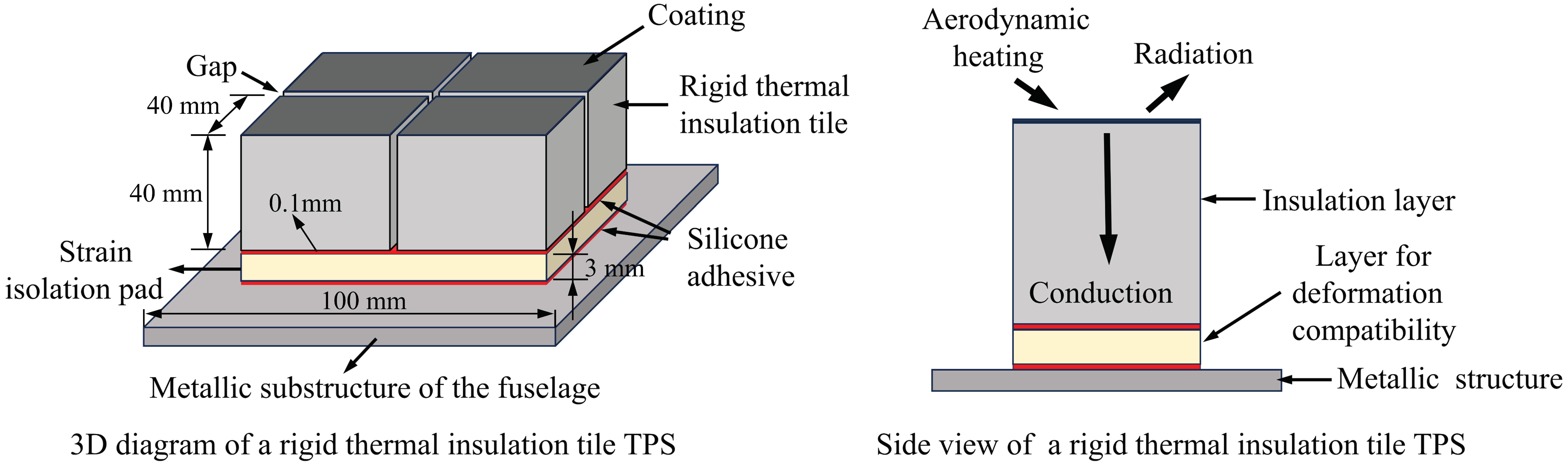
1. Introduction
2. Experiment
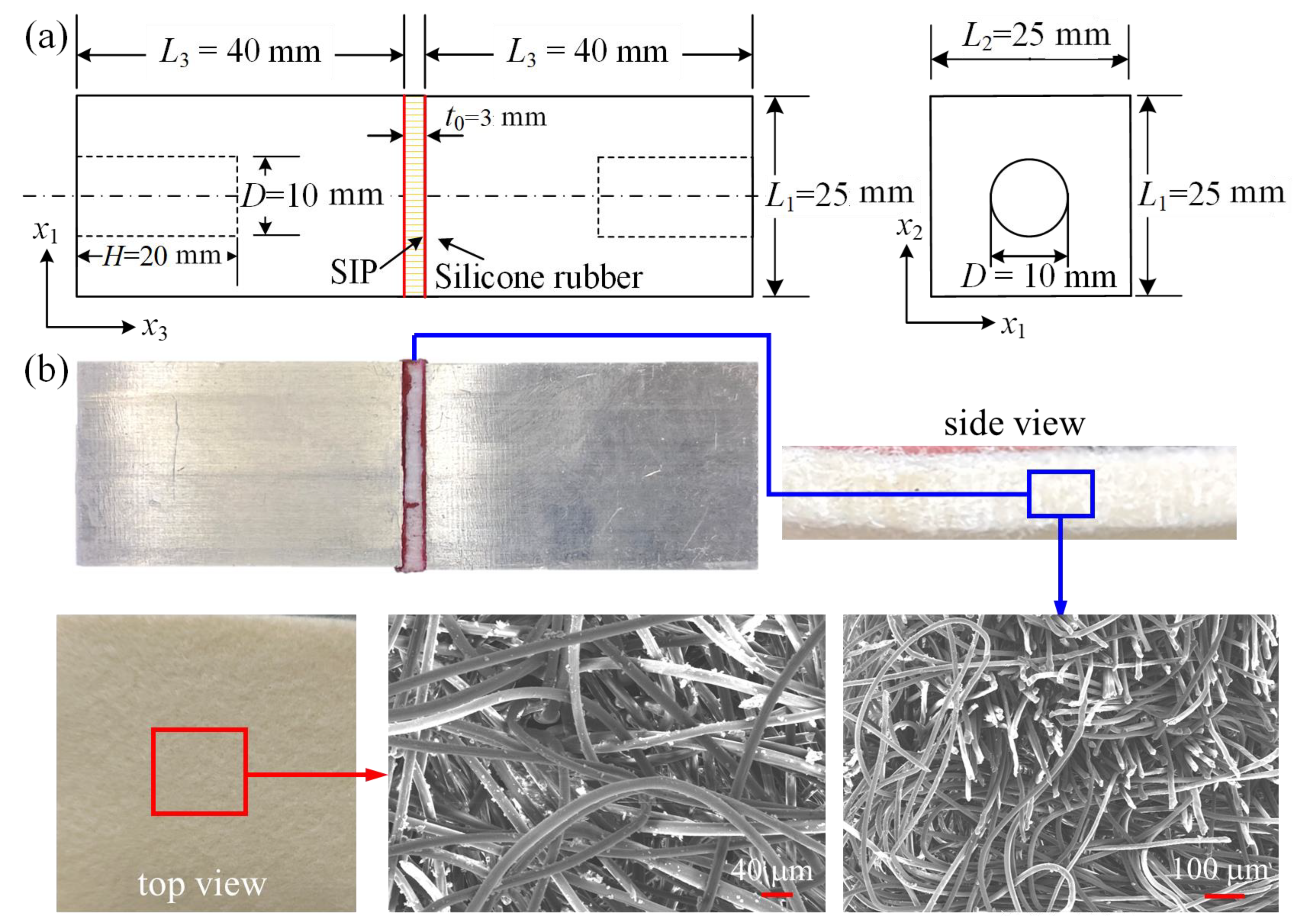
2.1. Material and Specimen
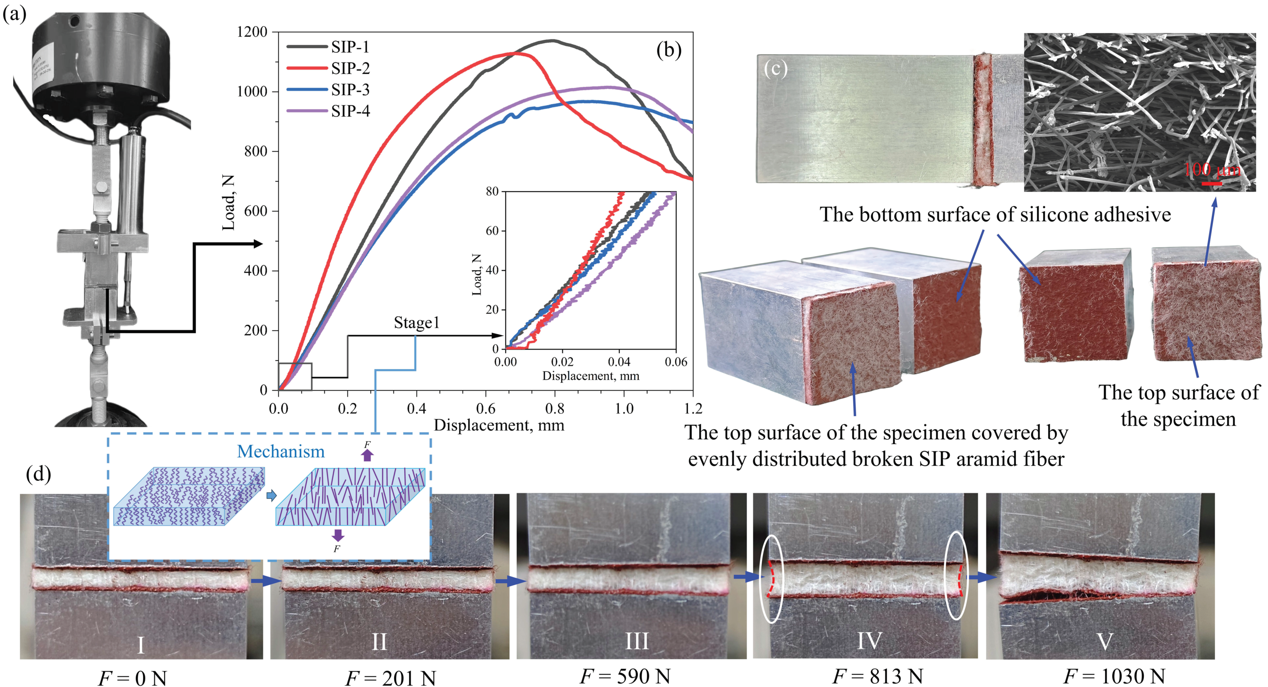
2.2. Experimental Setup
3. Monotonic Through-Thickness Tension
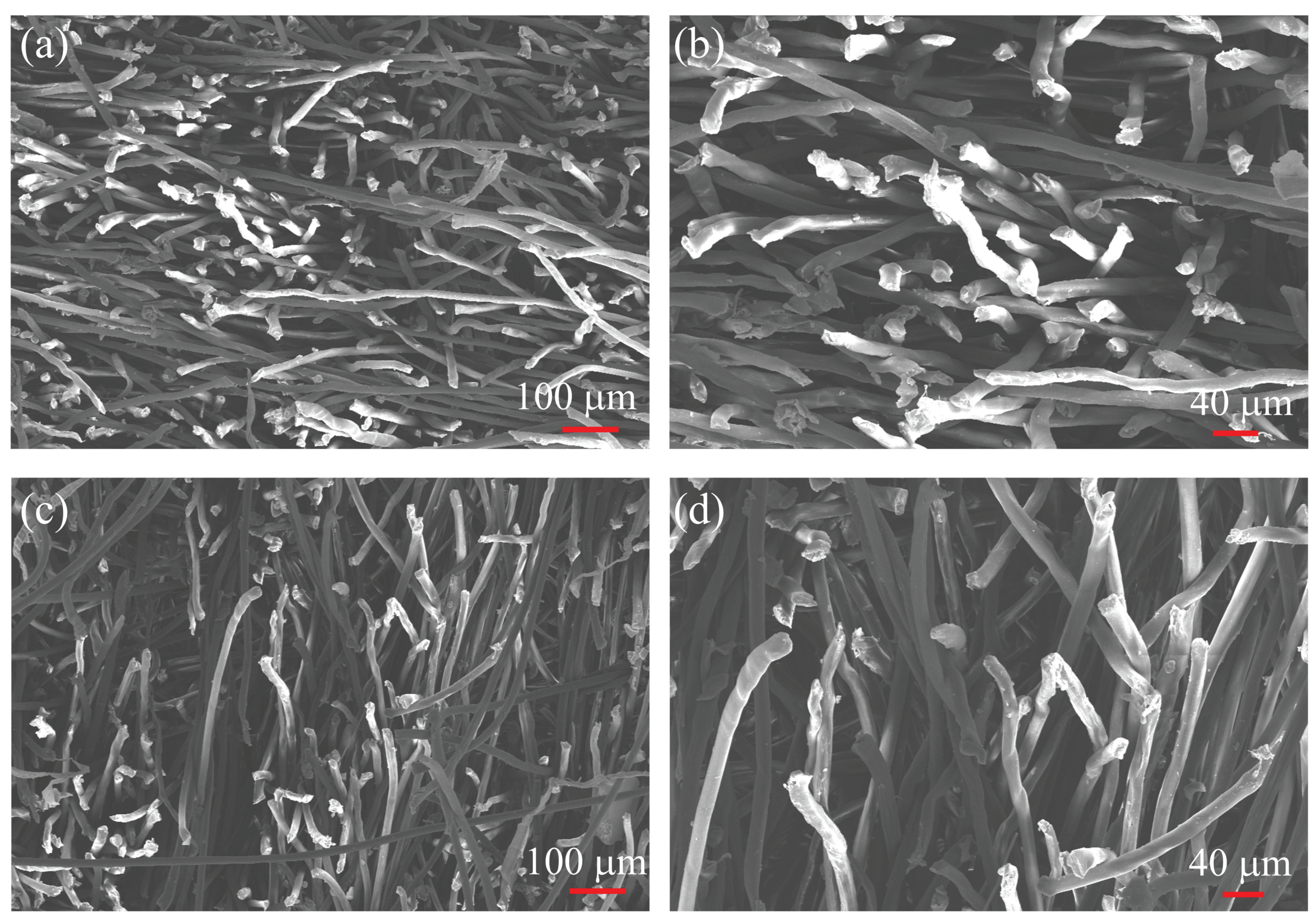
3.1. Test Results
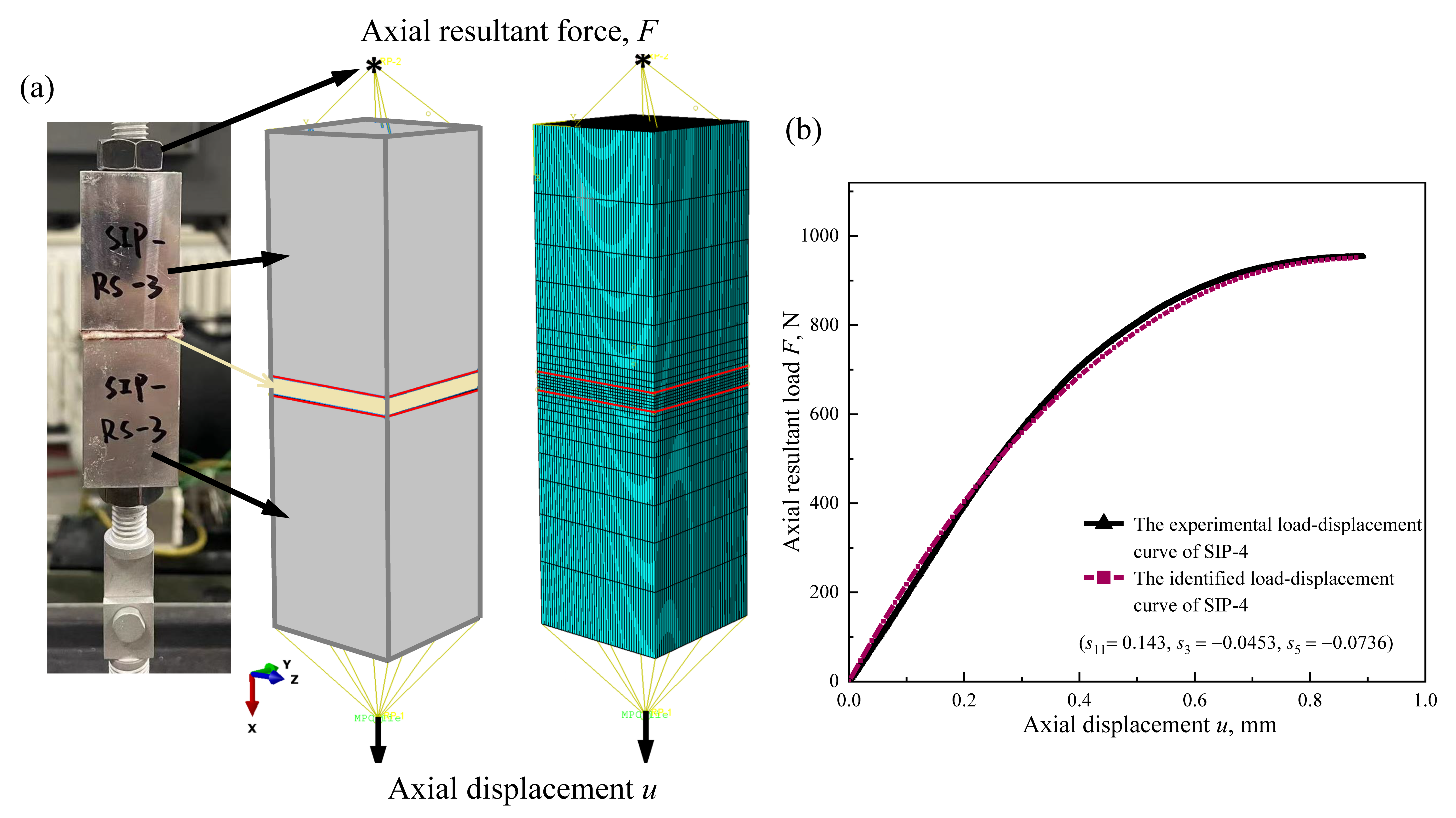
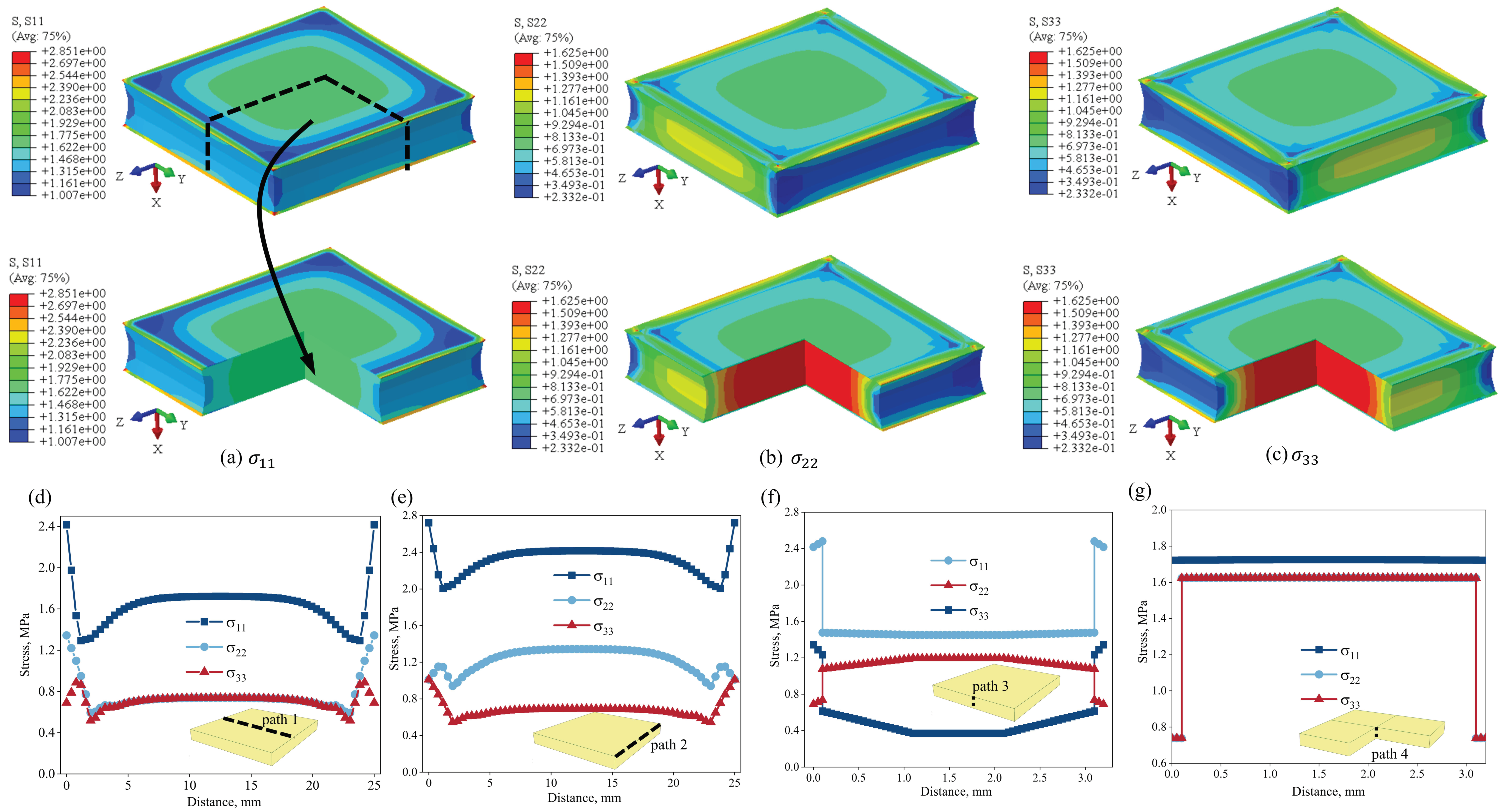
3.2. The Nonlinear Stress–Strain Relationship under Through-Thickness Tension
4. Tensile Fatigue Tests
4.1. The Loading–Unloading Tensile Response with Ratcheting Effect
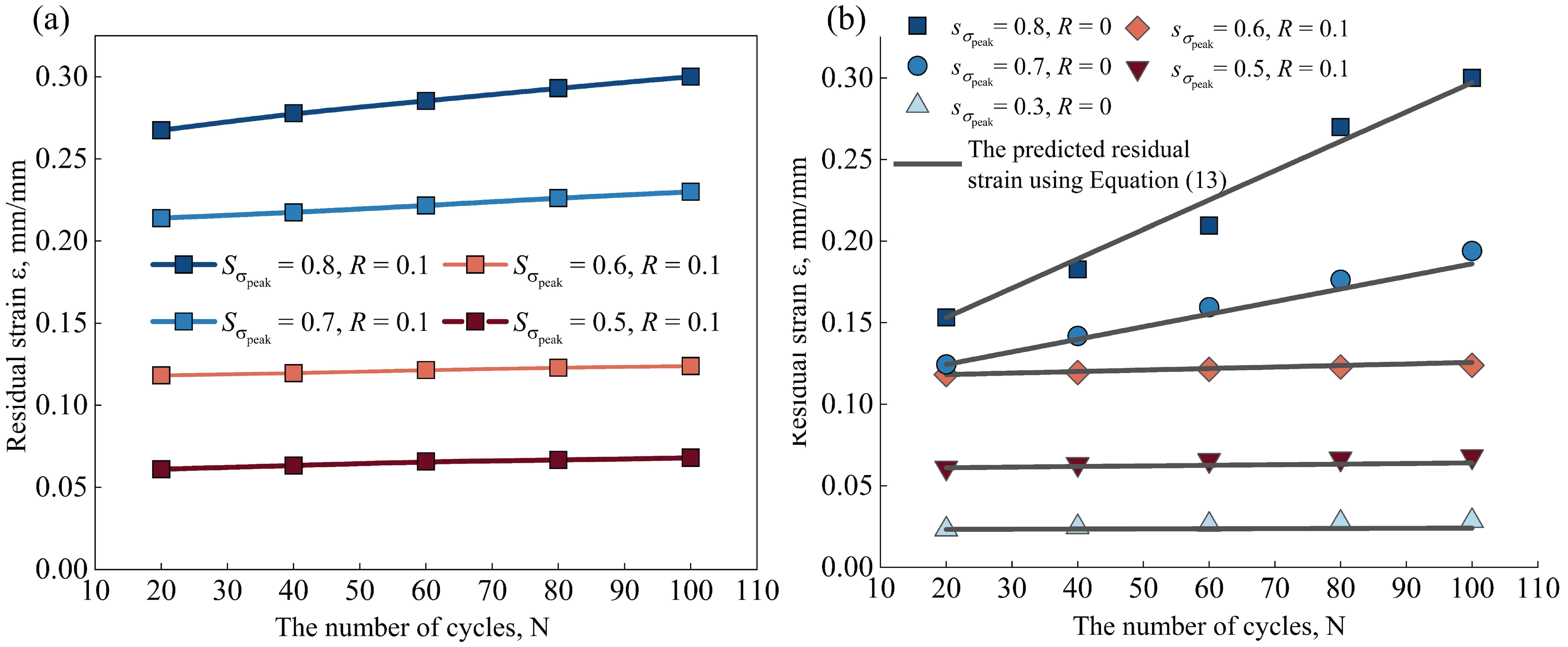
4.2. High Cycle Fatigue Test Results
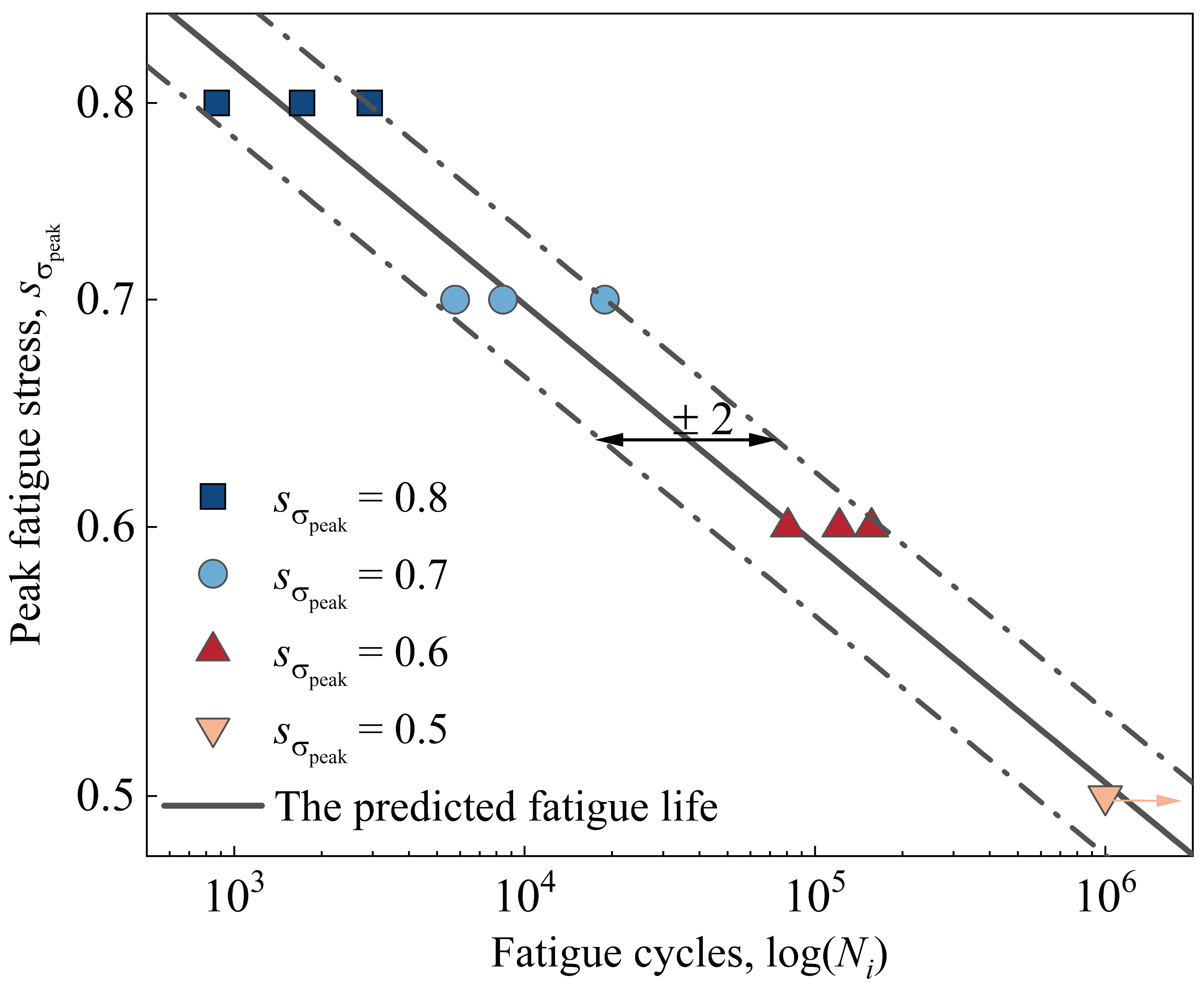
4.3. Prediction of Tensile Fatigue Life
5. Conclusions
Author Contributions
Funding
Data Availability Statement
Conflicts of Interest
References
- Petley, D.; Alexander, W.; Ivey, G.; Kerr, P.A. Steady Internal Flow and Aerodynamic Loads Analysis of Shuttle Thermal Protection System; Technical Report NASA/TP-1984-2255; NASA Langley Research Center: Hampton, VA, USA, 1984.
- Qin, Q.H.; Xu, J.L.; Guo, S. Fluid–thermal analysis of aerodynamic heating over spiked blunt body configurations. Acta Astronaut. 2016, 132, 230–242. [Google Scholar] [CrossRef]
- McNamara, J.J.; Thuruthimattam, B.J.; FriedFmann, P.P.; Powell, K.; Bartels, R. Hypersonic aerothermoelastic studies for reusable launch vehicles. In Proceedings of the 45th AIAA/ASME/ASCE/AHS/ASC Structures, Structural Dynamics and Materials Conference, Palm Springs, CA, USA, 19–22 April 2004; p. 1590. [Google Scholar]
- Glass, D.E. Ceramic matrix composite (CMC) thermal protection systems (TPS) and hot structures for hypersonic vehicles. In Proceedings of the 15th AIAA International Space Planes and Hypersonic Systems and Technologies Conference, Dayton, OH, USA, 28 April–1 May 2008; p. 2682. [Google Scholar]
- Wu, D.F.; Wang, Y.W.; Gao, Z.; Yang, J. Insulation performance of heat-resistant material for high-speed aircraft under thermal environments. J. Mater. Eng. Perform. 2015, 24, 3373–3385. [Google Scholar] [CrossRef]
- Dwoyer, D.L.; Newman, P.A.; Thames, F.C.; Melson, N.D. A Tile-Gap Flow Model for Use in Aerodynamic Loads Assessment of Space Shuttle Thermal Protection System: Parallel Gap Faces; Technical Report NASA/TM-1981-83151; NASA Langley Research Center: Hampton, VA, USA, 1981.
- Walker, J.D. From Columbia to discovery: Understanding the impact threat to the space shuttle. Int. J. Impact. Eng. 2009, 36, 303–317. [Google Scholar] [CrossRef]
- Eason, T.G.; Spottswood, S. A structures perspective on the challenges associated with analyzing a reusable hypersonic platform. In Proceedings of the 54th AIAA/ASME/ASCE/AHS/ASC Structures, Structural Dynamics, and Materials Conference, Boston, MA, USA, 8–11 April 2013; p. 1747. [Google Scholar]
- Sanders, B.J. The Need for a Versatile & Reusable Hypersonic Vehicle. In Proceedings of the 55th International Astronautical Congress of the International Astronautical Federation, the International Academy of Astronautics, and the International Institute of Space Law, Vancouver, BC, Canada, 4–8 October 2004; p. S-5-03. [Google Scholar]
- Chen, Y.; Li, D.; Sun, C.C.; He, Y.L. Response characteristics of thermal-mechanical coupling in rigid ceramic insulation tiles. J. Eng. Thermophys. 2020, 41, 3021–3029. [Google Scholar]
- Sawyer, J.; Rummler, D. Room Temperature Mechanical Properties of Shuttle Thermal Protection System Materials; Technical Report NASA/TM-1980-81786; NASA Langley Research Center: Hampton, VA, USA, 1980.
- Phillips, E. Tension-Tension Fatigue Behavior of the Space Shuttle Strain-Isolation-Pad Material; Technical Report NASA/TM-1980-83183; NASA Langley Research Center: Hampton, VA, USA, 1981.
- Kong, B.; Yang, J.Y.; Wang, M.; Zhang, Q.; Huang, J.; Yao, W. Experiments on high temperature mechanical properties and stress distribution laws on strain isolation pad. J. Northwestern Polytech. Univ. 2018, 36, 1162–1167. [Google Scholar] [CrossRef]
- Huang, J.; Yao, W.X. High-temperature mechanical properties of strain isolation pad for thermal protection system. J. Spacecr. Rocket. 2018, 55, 848–855. [Google Scholar] [CrossRef]
- Huang, J.; Yao, W.X.; Li, P.; Zhou, D.; Chang, C.; Lin, H. Investigation on dynamic behaviors of thermal protection system using a two degree-of-freedom nonlinear theoretical method. Acta Astronaut. 2018, 151, 828–835. [Google Scholar] [CrossRef]
- Villar-Rodil, S.; Martińez-Alonso, A.; Tascón, J.M. Studies on pyrolysis of Nomex polyaramid fibers. J. Anal. Appl. Pyrol. 2001, 58, 105–115. [Google Scholar] [CrossRef]
- Perepelkin, K.E.; Andreeva, I.V.; Pakshver, E.A.; Morgoeva, I.Y. Thermal characteristics of para-aramid fibres. Fibre Chem. 2003, 35, 265–269. [Google Scholar] [CrossRef]
- Cao, K.K.; Liu, Y.F.; Yang, Y.Y.; Yuan, F.; Wang, J.; Liu, H.; Jiang, M.; Yang, J. The preparation and characterization of a heterocyclic meta-aramid fiber with outstanding thermal stability. High Perform. Polym. 2021, 33, 554–567. [Google Scholar] [CrossRef]
- ASTM C297/C297M-04; Standard Test Method for Flatwise Tensile Strength of Sandwich Constructions. ASTM International: West Conshohocken, PA, USA, 2004.
- Cognard, J.Y. Numerical analysis of edge effects in adhesively-bonded assemblies application to the determination of the adhesive behaviour. Comput. Struct. 2008, 86, 1704–1717. [Google Scholar] [CrossRef]
- Cognard, J.Y.; Devaux, H.; Soheir, L. Numerical analysis and optimisation of cylindrical adhesive joints under tensile loads. Int. J. Adhes. Adhes. 2010, 30, 706–719. [Google Scholar] [CrossRef]
- Wang, W.X.; Takao, Y. A nonlinear elastic stress-strain relation of orthotropic composite plates. Acta Mech. Solida Sin. 1991, 12, 253–358. [Google Scholar]
- Ji, X.H.; Hao, Z.Q.; Su, L.J.; He, T.; Liu, L. Characterizing the constitutive response of plain-woven fibre reinforced aerogel matrix composites using digital image correlation. Compos. Struct. 2020, 234, 111652. [Google Scholar] [CrossRef]
- Lecompte, D.; Snits, A.; Vantomme, J.; Vantomme, J.; Van Hemelrijck, D. Mixed numerical–experimental technique for orthotropic parameter identification using biaxial tensile tests on cruciform specimens. Int. J. Solids Struct. 2007, 44, 1643–1656. [Google Scholar] [CrossRef]
- Ereiz, D.; Duvnjak, I.; Jiménez-Alonso, J.F. Review of finite element model updating methods for structural applications. Structures 2022, 41, 684–723. [Google Scholar] [CrossRef]
- Girardi, M.; Padovani, C.; Pellegrini, D.; Robol, L. A finite element model updating method based on global optimization. Mech. Syst. Signal Process. 2021, 152, 107372. [Google Scholar] [CrossRef]
- Xiao, H.R.; Cai, L.X.; Han, G.Z. A novel theoretical model for obtaining Norton’s law of creep materials using different small specimens. Int. J. Mech. Sci. 2023, 261, 108677. [Google Scholar] [CrossRef]
- Wu, K.; Shao, Z.; Qin, S.; Zhao, N.; Chu, Z. An improved nonlinear creep model for rock applied to tunnel displacement prediction. Int. J. Appl. Mech. 2021, 13, 2150094. [Google Scholar] [CrossRef]
- Sun, S. Study on the creep behavior of recombinant bamboo based on a modified generalized Kelvin model. Wood Sci. Technol. 2022, 56, 589–601. [Google Scholar]


| No-1 | No-2 | No-3 | No-4 | Mean | Standard Deviation | COV, % | |
|---|---|---|---|---|---|---|---|
| Peak stress, MPa | 1.87 | 1.55 | 1.62 | 1.81 | 1.71 | 0.11 | 6.6 |
| Peak strain, mm/mm | 0.26 | 0.3 | 0.32 | 0.23 | 0.28 | 0.035 | 12.5 |
| Fatigue Life, | |
|---|---|
| 0.8 | 1713; 872; 2932 |
| 0.7 | 8426; 18,897; 5763 |
| 0.6 | 80,728; 156,507; 121,381 |
| 0.5 | 999,815; run-out; run-out |
| 0.3 | run-out |
Disclaimer/Publisher’s Note: The statements, opinions and data contained in all publications are solely those of the individual author(s) and contributor(s) and not of MDPI and/or the editor(s). MDPI and/or the editor(s) disclaim responsibility for any injury to people or property resulting from any ideas, methods, instructions or products referred to in the content. |
© 2024 by the authors. Licensee MDPI, Basel, Switzerland. This article is an open access article distributed under the terms and conditions of the Creative Commons Attribution (CC BY) license (https://creativecommons.org/licenses/by/4.0/).
Share and Cite
Lu, M.; Wu, Z.; Hao, Z.; Liu, L. Experimental Investigation of the Mechanical Behavior of the Strain Isolation Pad in Thermal Protection Systems under Tension. Aerospace 2024, 11, 305. https://doi.org/10.3390/aerospace11040305
Lu M, Wu Z, Hao Z, Liu L. Experimental Investigation of the Mechanical Behavior of the Strain Isolation Pad in Thermal Protection Systems under Tension. Aerospace. 2024; 11(4):305. https://doi.org/10.3390/aerospace11040305
Chicago/Turabian StyleLu, Maoxu, Zhenqiang Wu, Ziqing Hao, and Liu Liu. 2024. "Experimental Investigation of the Mechanical Behavior of the Strain Isolation Pad in Thermal Protection Systems under Tension" Aerospace 11, no. 4: 305. https://doi.org/10.3390/aerospace11040305
APA StyleLu, M., Wu, Z., Hao, Z., & Liu, L. (2024). Experimental Investigation of the Mechanical Behavior of the Strain Isolation Pad in Thermal Protection Systems under Tension. Aerospace, 11(4), 305. https://doi.org/10.3390/aerospace11040305