Abstract
With reference to the trajectory-based operation (TBO) requirements proposed by the International Civil Aviation Organization (ICAO), this paper concentrates on the study of four-dimensional trajectory (4D Trajectory) prediction technology in busy terminal airspace, proposing a data-driven 4D trajectory prediction model. Initially, we propose a Spatial Gap Fill (Spat Fill) method to reconstruct each aircraft’s trajectory, resulting in a consistent time interval, noise-free, high-quality trajectory dataset. Subsequently, we design a hybrid neural network based on the seq2seq model, named Attention-TCN-GRU. This consists of an encoding section for extracting features from the data of historical trajectories, an attention module for obtaining the multilevel periodicity in the flight history trajectories, and a decoding section for recursively generating the predicted trajectory sequences, using the output of the coding part as the initial input. The proposed model can effectively capture long-term and short-term dependencies and repetitiveness between trajectories, enhancing the accuracy of 4D trajectory predictions. We utilize a real ADS-B trajectory dataset from the airspace of a busy terminal for validation. The experimental results indicate that the data-driven 4D trajectory prediction model introduced in this study achieves higher predictive accuracy, outperforming some of the current data-driven trajectory prediction methods.
1. Introduction
As the aviation sector expands swiftly and flight frequencies rise, the complexity of air traffic management is also increasing. The characteristics of air traffic include high traffic volume, dense flight activities, and small intervals between flights. Europe and the United States have proposed trajectory-based operations (TBO) to increase airspace resource utilization and achieve precise flight control. As TBO gain increasing popularity, the need for highly accurate trajectory prediction is becoming more critical not only for optimising airspace resources but also for enhancing air traffic management efficiency and reducing flight delays. This precision in trajectory forecasting is vital for the improvement of advanced air traffic flow management (ATFM), enabling more effective utilization of airspace and ensuring smoother, more reliable flight operations. And accurate prediction of the 4D trajectories (latitude, longitude, altitude, and time) of aircraft in the terminal airspace of airports can help ATFM make better decisions, including adjusting aircraft routes and altitudes in order to avoid conflicts and congestion among aircraft, which can significantly diminish the unpredictability of future trajectories and enhance the foreseeability of air traffic. In this context, 4D trajectory prediction in the terminal airspace has significant research and application value for the aviation field. Significant foundational research has been conducted in the field of flight trajectory prediction from an early stage. For instance, Chatterji [1] achieved short-term trajectory prediction by estimating future states of an aircraft based on its current state. Gong et al. [2] introduced an automatic trajectory prediction analysis method that could record, segment, and eliminate outliers in trajectory data automatically. Lymperopoulos et al. [3] developed a prediction algorithm for aircraft take-off trajectories, establishing a state estimation model that incorporates weather and wind direction information. Rentas et al. [4] analysed methods for evaluating trajectory prediction outcomes and the predictive capabilities of models. Mondoloni et al. [5] constructed a statistical model for forecasting wind field uncertainties, analysing the impact of initial conditions such as wind strength on trajectory predictions. Klooster et al. [6] proposed a control method for four-dimensional time-based operations (TBO) that integrates temporal controls. Leege et al. [7] employed machine-learning techniques to build regression prediction models for trajectory prediction. Fablec et al. [8] introduced a trajectory prediction method based on neural networks, laying the theoretical groundwork for the numerous neural-network-based trajectory prediction models that are prevalent today. Overall, these early studies have provided essential technical support for trajectory prediction. Presently, the primary focus of research on 4D trajectory prediction is grounded in three types of methods: dynamics modelling, state estimation, and data-driven methods.
The method of trajectory prediction using dynamics modelling mainly regards the aircraft as a mass point and predicts the possible points of the future trajectory using the force acting on the aircraft to achieve the 4D trajectory prediction. Thipphavong et al. [9] enhanced the accuracy of trajectory predictions during an aircraft’s climb phase by dynamically adjusting the aircraft weight in the dynamic equations, using real-time trajectory datasets. Han Yunxiang et al. [10] proposed a dynamics model based on each navigation stage to infer the trajectory using parameters such as aircraft mass and speed. However, these fixed prediction methods do not consider the uncertainty of the navigation environment, which reduces the prediction accuracy.
The state estimation method converts the problem of predicting aircraft trajectories into a state transfer problem in a mathematical model. Liu and Hwang [11] combined aircraft intent information and proposed a stochastic linear hybrid system that jointly describes flight mode changes using state-dependent transition models and Markov transition models, achieving more accurate aircraft prediction results. Ayhan and Samet [12] employed 4D cubes to represent trajectories by incorporating flight alignment and fusion processes, and they proposed the Hidden Markov Model (HMM).
With the continuous progress of big data theory, data-driven trajectory prediction models show excellent prediction performance; they can actively recognize and capture complex patterns and relationships in the data, avoiding the complexity of traditional model parameter settings and the constraints of environmental adaptability, and have become key 4D trajectory prediction tools. Such a model transforms the difficult problem of trajectory prediction into a time-series prediction problem by mining feature information from a large amount of data and integrating these features to find their internal associations. Wang et al. [13] proposed a model to solve the problem of predicting short-term trajectories in terminal airspace using machine-learning techniques, namely trajectory clustering and a BP (back propagation) neural network. But the model’s oversimplified structure makes it difficult to capture flight patterns in complex terminal airspace. Hernández et al. [14] used a traditional integrated machine-learning algorithm for aircraft trajectory prediction. Barratt et al. [15] developed two separate and related prediction models by dividing the set of trajectories in airport terminal airspace according to take-off and landing procedures. The method uses a clustering model to mine flight patterns in ADS-B data and finally realizes the trajectory prediction. Hong et al. [16] constructed a linear regression function for the trajectory prediction problem and utilized a multivariate mixed regression model, combining it with machine learning to achieve the prediction of flight trajectories.
Alligier et al. [17] applied a deep-learning approach to mine the operating laws of historical trajectories in order to achieve high-precision prediction of aircraft climb phases. Pang et al. [18] established convolutional neural networks (CNN) and fully connected layer neural networks (FCNN) using machine-learning theory to achieve high-accuracy trajectory predictions. Shi et al. [19] proposed a constrained long short-term memory network (LSTM) for trajectory prediction using the flight characteristics in each phase of an aircraft flight as constraints. Fan Zhonghang et al. [20] analysed the relationship between aircraft manoeuvring characteristics and trajectory prediction and, based on this, proposed a trajectory prediction method based on a residual recurrent neural network (RESRNN). Tran et al. [21] proposed a deep-learning model that reasonably avoids the data effects of aircraft performance and meteorological elements, and achieves more accurate trajectory predictions through modelling and combining aircraft intent information. Wang et al. [22] proposed a hybrid neural network for long-term prediction of trajectories: the TraNet model. The model consists of multiple modules that process long- and short-term information, which can better capture the global trajectory information and thus yield more accurate long-term trajectory predictions. Zeng Weili et al. [23] introduced the seq2seq theory into trajectory prediction and proposed a deep long short-term memory network (SS-DLSTM) based on this theory to achieve higher-accuracy trajectory predictions. Lim Zhi Jun et al. [24] and Lui, Go Nam et al. [25] considered terminal-area congestion and other anomalies, and modelled flight speed control for delay prediction and arrival time prediction, respectively.
While numerous experts have proposed a variety of 4D trajectory prediction methods, current models often struggle to achieve high performance in the complex and busy terminal airspace environment. A critical review of existing literature reveals two predominant challenges. Firstly, some models do not consider unmodeled behavioural features in historical trajectories, and the extreme complexity of some models leads to long training periods, reducing their practicality for real-time applications. Secondly, other models feature simpler network structures that fail to capture the full complexity of input trajectory sequences. These models struggle to understand the intricate patterns and dependencies within long sequences, essential for accurate trajectory predictions. This research aims to address these shortcomings by developing a balanced approach that optimizes model complexity to reduce training time while enhancing the model’s ability to grasp the detailed dynamics of trajectory sequences in busy terminal airspace, thereby improving prediction accuracy and practical applicability.
In order to solve these problems mentioned above, this paper proposes a 4D trajectory prediction model for terminal airspace based on Attention-TCN-GRU. This model employs TCN and GRU neural networks as encoder and decoder, respectively, and incorporates attention mechanisms. By modelling historical flight data, it achieves the prediction of the 4D trajectories of aircraft in terminal airspace. The model is capable of effectively understanding and processing complex patterns in long trajectory sequences. It focuses on the operational feature information in different parts of the input trajectory sequences, significantly enhancing the predictive performance in terms of terminal airspace 4D trajectories.
The important contributions of this paper are as follows: (1) Aiming at problems such as outliers and vacancies in the received raw trajectory set, this study introduces the Spat Fill method, reconstructing the original trajectories into high-quality data with equal time intervals. (2) Considering the before-and-after information dependence of the trajectory sequence and the prediction performance, this paper introduces the Attention-TCN-GRU model, which is tailored to the characteristics of terminal airspace and is better suited for 4D trajectory prediction within terminal airspace. (3) For the dataset, this paper divides the trajectory data according to busy times and idle times, which avoids the mutual interference between busy time and idle time trajectories and is conducive to improving the prediction performance.
The rest of the paper is organized as follows. Section 2 describes the analysis and preprocessing of the data. Section 3 describes the data-driven prediction method for 4D trajectories. Section 4 analyses the performance of the model in this paper through experiments and compares and analyses it with other mainstream models. Finally, the results are summarized in Section 5.
2. Data Analysis and Processing
The automatic broadcast-dependent surveillance system (ADS-B) [26] used in this paper is a new satellite-based air traffic control paradigm for connecting aircraft with ground stations. The system utilizes satellites to automatically and continuously provide 4D position data (latitude, longitude, and time), while altitude, speed, and heading information are provided by onboard aircraft equipment. Subsequently, these data are transmitted to ground receiving stations via ADS-B signals and saved by the ground receiving stations. These historical ADS-B data are key to 4D trajectory prediction using data-driven methods. Each data item consists of several attributes including flight number, time, latitude, longitude, altitude, speed, heading, and aircraft type. Considering the problem that the prediction performance of the deep-learning model for time-series data decreases with the length of the data, in this paper, position measurements within the centre of the airport that are less than 20 km distant and less than 6000 feet in altitude are retained. The data range starts from the tail end of the initial approach phase and completely includes the intermediate and final approach phases.
In the field of civil aviation, an aircraft undergoes seven distinct flight phases during a single operation: take-off, climb, departure, enroute flight, arrival, approach, and landing. For arriving aircraft, the focus is primarily on the arrival, approach, and landing phases, with some aircraft requiring a go-around phase.
- Arrival Phase: The arrival phase marks the transition of the aircraft from enroute to the terminal area boundary, culminating at the initial approach fix (IAF), where the aircraft changes its mode of air travel. Aircraft at different altitudes can intersect with the same arrival route, with each aircraft utilising different flight levels. This phase requires adherence to both vertical and horizontal separation standards, with the majority of sequencing completed during this stage.
- Approach Phase: This phase encompasses the initial, intermediate, and final approach. Aircraft descend from the IAF, reducing altitude and speed according to prescribed approach procedures. Adjustments to horizontal separation are made based on intersecting flight paths to avoid conflicts, aiming first for the intermediate fix (IF) point, then maintaining altitude and speed without deviating from the course to reach the final approach fix (FAF) point, and finally landing on the runway.
- Landing and Go-Around Phase: Aircraft that do not meet landing criteria or fail to land successfully undergo a go-around procedure. The aircraft will either fly back to the IAF for another approach, circle in a designated holding area, or climb to a minimum safe altitude for another landing attempt.
- For departing aircraft, the take-off and departure phases are considered.
- Take-off Phase: This phase marks the commencement of the flight. The aircraft accelerates on the runway until it reaches sufficient speed to generate the necessary lift for take-off. The take-off process involves complex control and system checks to ensure safe departure.
- Departure Phase: Once airborne, the aircraft enters the departure phase, following predetermined flight paths to leave the vicinity of the airport. This stage may involve changes in direction, altitude, and speed to smoothly integrate the aircraft into higher airspace traffic flows. Air traffic control (ATC) plays a crucial role during this phase, guiding the aircraft to avoid conflicts with other flights and ensuring it follows the planned route.
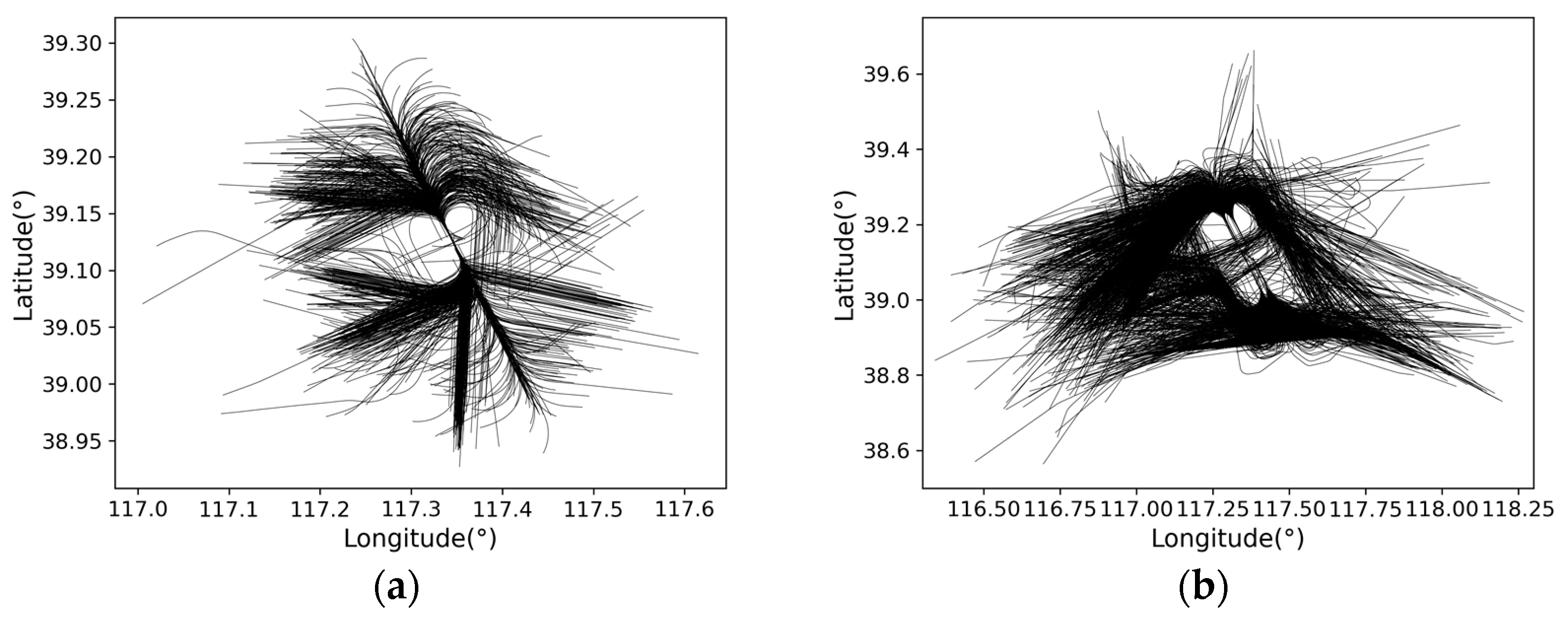
For arriving aircraft, the arrival phase altitude ranges from 30,000 to 3000 feet, with the approach phase below 3000 feet, including the altitude range for go-arounds. Departing aircraft typically operate within a 5000 to 6000 feet range during the departure phase. Considering the diminishing predictive performance of deep-learning models with increasing data length, a height range of 0–6000 feet and a latitude and longitude range of 20 km are selected. The arrival trajectory covers the end of the arrival phase and the entire approach phase, enabling 4D trajectory prediction from the initial approach fix onwards for both the terminal end of the arrival phase and the entire approach phase. For departing trajectories, it is possible to predict the 4D trajectory of aircraft from runway take-off to leaving the terminal area and entering the climb phase. This research holds practical significance for future conflict resolution, enhancing terminal area operational efficiency, and adjustments to flight procedures and approach fixes. The data used in this article come from a real terminal area, with latitude between 38 and 42° north and longitude between 115 and 120° east. The ADS-B track data coordinate system used in this paper is the World Geodetic System-84 (WGS-84) coordinate system. Figure 1 shows a visualization of the historical trajectory within the terminal area after the dataset is divided into take-off and landing trajectories.
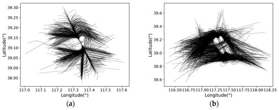
Figure 1.
Visualization of trajectory data. (a) Visualization of take-off trajectory; (b) Visualization of landing trajectory.
2.1. Data Collection
Flight trajectories are influenced by a multitude of complex processes including flight dynamics, avionics, operational constraints, decisions made at the Air Navigation Service Provider (ANSP) level, and weather conditions. Our data-driven 4D trajectory prediction model significantly reduces the complexity of parameters, avoiding the use of actual operational parameters such as flight dynamics, and is entirely based on historical ADS-B data to achieve high-precision trajectory predictions.
ADS-B historical track data are discontinuous and are broadcast almost every second from equipped aircraft. The ADS-B data used in this paper come from a large airport (approximate location provided due to confidentiality: north latitude range 38–42, east longitude range 115–120), totalling more than four thousand take-off and landing trajectories.
The problem of predicting airplane flight trajectories is defined as a regression problem. In this research task, it is assumed that the set of historical trajectories T consists of N historical trajectories; it is represented by the following equation:
where is the number R track in M. Assuming that each trajectory has n waypoints, it is represented by the following equation:
where is the number i waypoint in . Assuming that each waypoint contains p attributes, it is represented by the following equation:
where denotes the number j attribute of the point. In this paper, we are using ADS-B data from a large airport containing the following track characteristics: = {time, flight number, latitude, longitude, altitude, speed, heading, pitch, roll}.
2.2. Data Preprocessing
In practice, ADS-B data may have various quality defects, such as bias in position information or missing data. This paper primarily addresses two key issues with the original flight trajectories in the ADS-B dataset. Firstly, certain trajectory data at specific time points may contain anomalies due to reasons such as noise. Secondly, the length of the time intervals is not constant. Efficient trajectory prediction requires high-quality data with equal time intervals as a foundation. The goal of trajectory reconstruction is to generate high-quality trajectories from low-quality ones. This paper introduces a method named “Spatial Gap Fill” (Spat Fill) for trajectory reconstruction. This method can discard outliers and reconstruct missing data based on their neighbouring points for all vacant values.
For the receiving trajectory F and the high-quality trajectory H, where denotes the high-quality track containing N equally spaced track points and denotes the receiving track containing M equally spaced track points, the following relationship exists between the two:
where Q denotes the sampling matrix and n denotes outliers such as noise and outliers. The trajectory reconstruction is to recover F to a high-quality track H. However, we cannot get the high-quality track directly from the above linear relationship, so the Spat Fill method is used for the trajectory reconstruction. The specific method is as follows:
For the treatment of outliers and other anomalies in trajectory sequences, this paper defines the point correlation of trajectory sequences. For each trajectory point in the sequence, we set a distance threshold “a” for its neighbourhood “G”, the “a” parameter serving to define the maximum accepted distance between data points. For each data point, we calculate the distance between it and all trajectory points within the neighbourhood and mark those exceeding the distance threshold as anomalies. Additionally, this paper defines the connectivity of trajectory points in different neighbourhoods to prevent two points with overly long distances on the trajectory sequence from being identified as outliers. The related formulaic expression is as follows.
G neighbourhood is a region of distance G from the data point in the trajectory sequence, and the data points contained in the region are considered to be in the neighbourhood of :
Two points are defined as having a trajectory sequence point correlation if the point in the neighbourhood of G and the centre point satisfy the following conditions.
If there is a track point, , that is correlated with the otherwise uncorrelated data points and , then the data points and are also correlated and belong to the same track sequence points and will not be recognized as outliers. After point correlation is identified for all track sequence points of a track sequence, the remaining points that are not attributed to correlation with this track sequence are identified as outliers.
The trajectory sequences, after removing the outliers, still have issues with varying time intervals and missing values. In this paper, we employ cubic spline interpolation to fill in the latitude, longitude, altitude, speed, and heading in the flight trajectories. After compensating for the missing values, we obtain high-quality trajectory data with equal time intervals, which facilitates the calculation of time errors through trajectory length. It also benefits the process of feeding these trajectory sequence features into the neural network model. By utilising neural networks to learn the operating patterns of trajectories in air routes, we achieve high-precision 4D trajectory predictions. As illustrated in Figure 2, a set of representative trajectories with anomalies and their reconstructed schematics are provided. Clearly, the reconstructed trajectories can handle anomalies and process trajectory time intervals effectively.
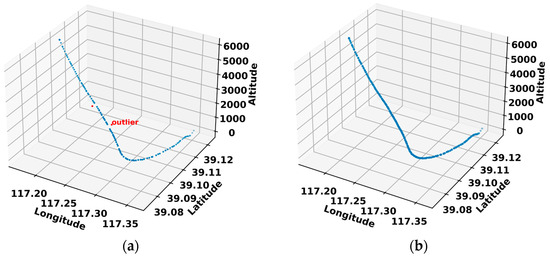
Figure 2.
Reconstruction diagram of a representative track with outlier. (a) Original trajectory; (b) reconstructed trajectory.
3. Methodology
3.1. 4D Trajectory Prediction Process
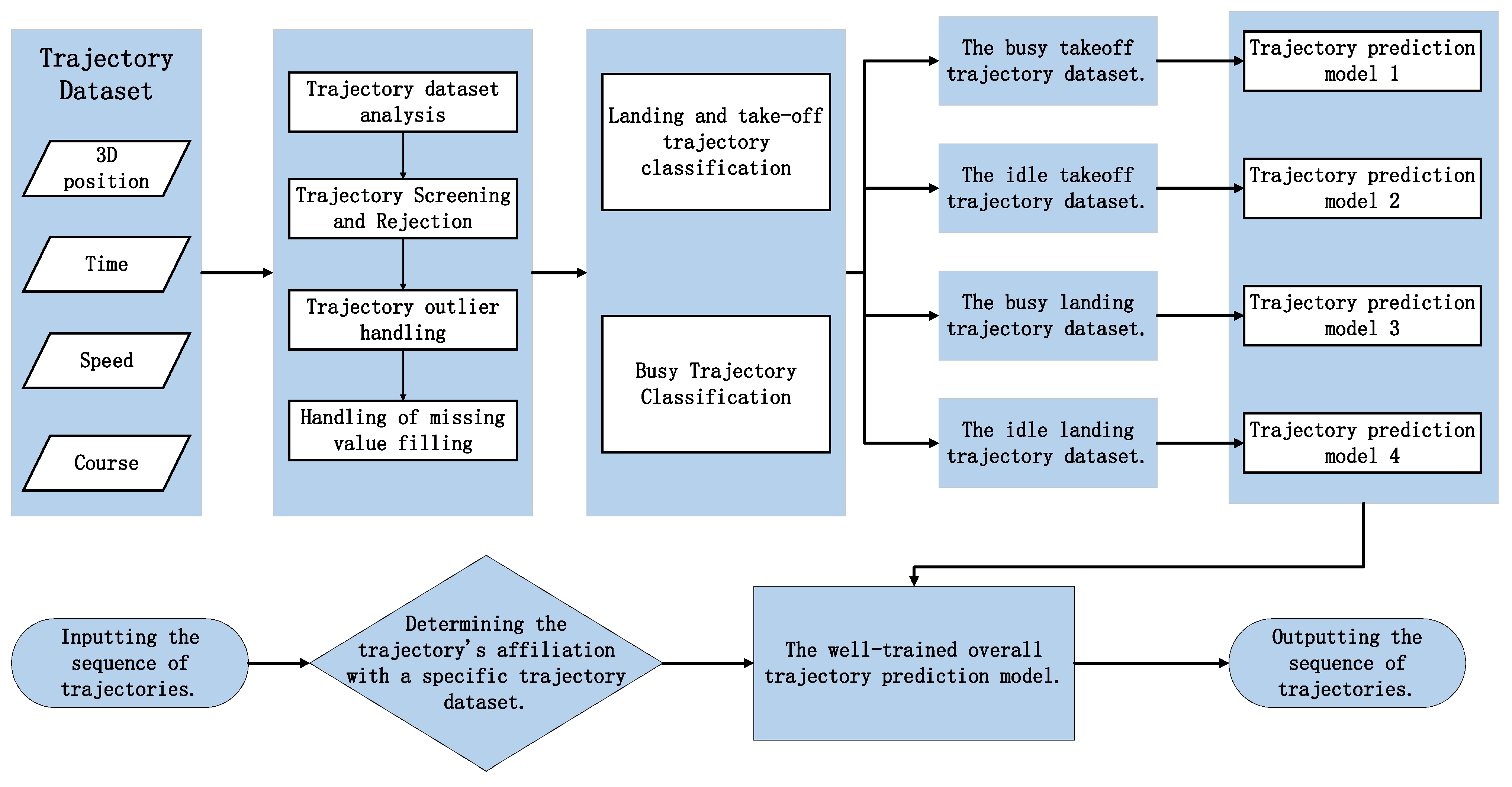
The use of data-driven approaches to machine learning is becoming more and more common due to the increasing demand for prediction tools. Realising efficient and accurate predictions of 4D trajectories in terminal airspace requires full consideration of the trajectory data characteristics, understanding the correlation among trajectories, and designing a reasonable deep model structure based on the trajectory characteristics. In this paper, we design an Attention-TCN-GRU model with a seq2seq structural framework for 4D trajectory prediction in terminal airspace. The overall prediction approach is depicted in Figure 3 and mainly consists of three stages:
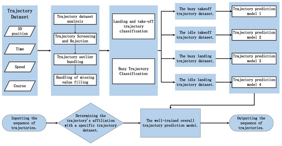
Figure 3.
4D trajectory prediction flowchart.
- Trajectory processing and categorization phase. Firstly, we renumber each trajectory under a specific flight number to ensure that each flight number corresponds to only one trajectory. Then, we filter trajectories based on a range within 20 km of the airport’s central point and below an altitude of 6000 feet. This filtering step aims to remove cruising and abnormal trajectories. Subsequently, we apply a Spatiotemporal Filling (Spat Fill) process to each trajectory to eliminate outliers and fill missing values, resulting in a high-quality trajectory dataset with consistent time intervals.
- Data set grouping training phase. We categorise the preprocessed high-quality trajectory dataset based on traffic density and different take-off and landing procedures. Therefore, we divide the trajectory dataset into take-off and landing groups and subject each group to traffic density analysis, resulting in datasets for busy and idle time periods. We divide each trajectory sequence into input and output sequences based on time. Due to variations in the duration of take-off and landing procedures, the lengths of input and output sequences for take-off and landing trajectories differ. Consequently, we train separate 4D trajectory prediction models for take-off and landing trajectories by inputting the trajectory sequences of each group into the designed Attention-TCN-GRU model.
- 4D trajectory prediction phase. For the required take-off or landing flights, we judge the busyness of the terminal airspace based on flight schedules. Subsequently, we input the trajectory sequences into the respective trained 4D trajectory prediction models to perform 4D trajectory predictions.
3.2. Attention-TCN-GRU Modeling
The model designed in this paper adopts the seq2seq architecture [27], and the following features indicate that this model architecture is particularly suitable for the 4D trajectory prediction problem in terminal airspace.
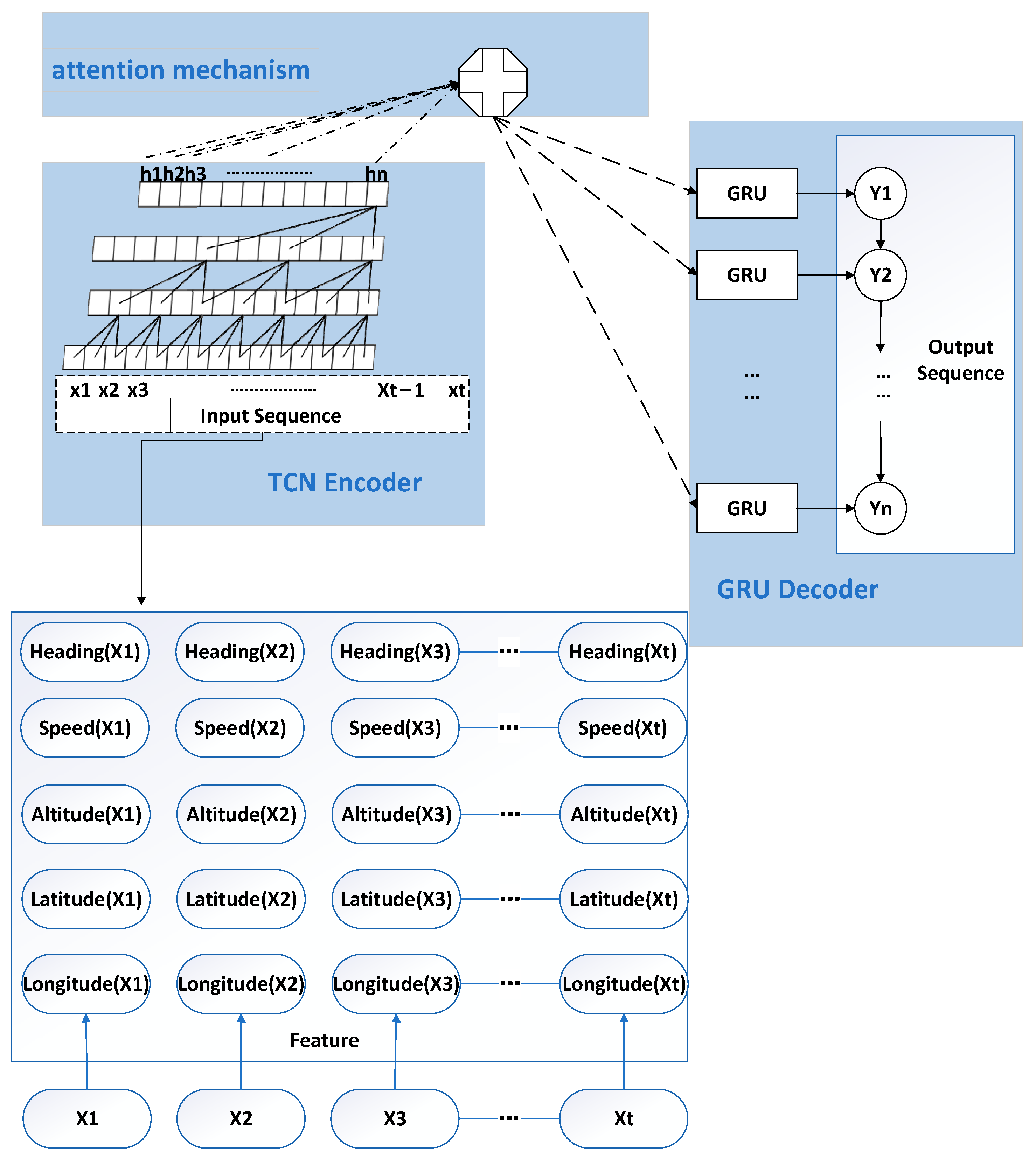
Initially, for 4D trajectory predictions in busy terminal airspace, since the aircraft has to follow certain flight procedures during take-off and landing, and each trajectory is a sequence of trajectories composed of a series of trajectory points, the trajectory prediction problem is introduced into the sequence-to-sequence architecture for processing and solving. Consequently, the seq2seq architecture can solve the length difference between the input and output trajectory data, which is just enough to fulfil the method of inputting short trajectory sequences to predict long trajectory sequences. Finally, the internal structures of the encoder and decoder are independent of each other. This suggests that they can be designed to perform different tasks. Thus, the encoder is trained to identify hidden information and patterns within the trajectory data. These pieces of information are outputted by the encoder as fixed-length context vectors, which are then dynamically linked by the decoder to output the predicted trajectories. The prediction model Attention-TCN-GRU in this paper is based on the theory of seq2seq models. It uses a TCN (temporal convolutional network) with better performance in processing long sequences as the encoder and a GRU (gated recurrent unit) with higher operational efficiency as the decoder, and it adds an attention mechanism to help the model pay better attention to important information in the fixed-length vectors output by the encoder. The methodology and overall architecture of the model are shown in Figure 4. Each part of the model is described in detail below.
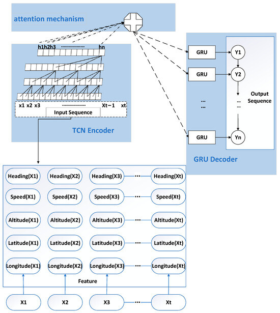
Figure 4.
4D trajectory prediction model based on Attention-TCN-GRU.
3.2.1. Trajectory Prediction Encoder TCN
The main function of the encoder designed in this paper is to learn and recognize the hidden patterns in aircraft input trajectory sequences. These hidden patterns contain information about aircraft characteristics under different operating environments, which is crucial for the prediction of the trajectory sequences. As a branch of convolutional networks, TCN is primarily employed for temporal data processing. This paper firstly employees a TCN network as an encoder for the task of 4D trajectory prediction in terminal airspace. It is adept at accurately learning both long and short dependencies within trajectory sequences, boasting ample memory capacity [28]. Thus, it retains more information and delivers enhanced encoding performance.
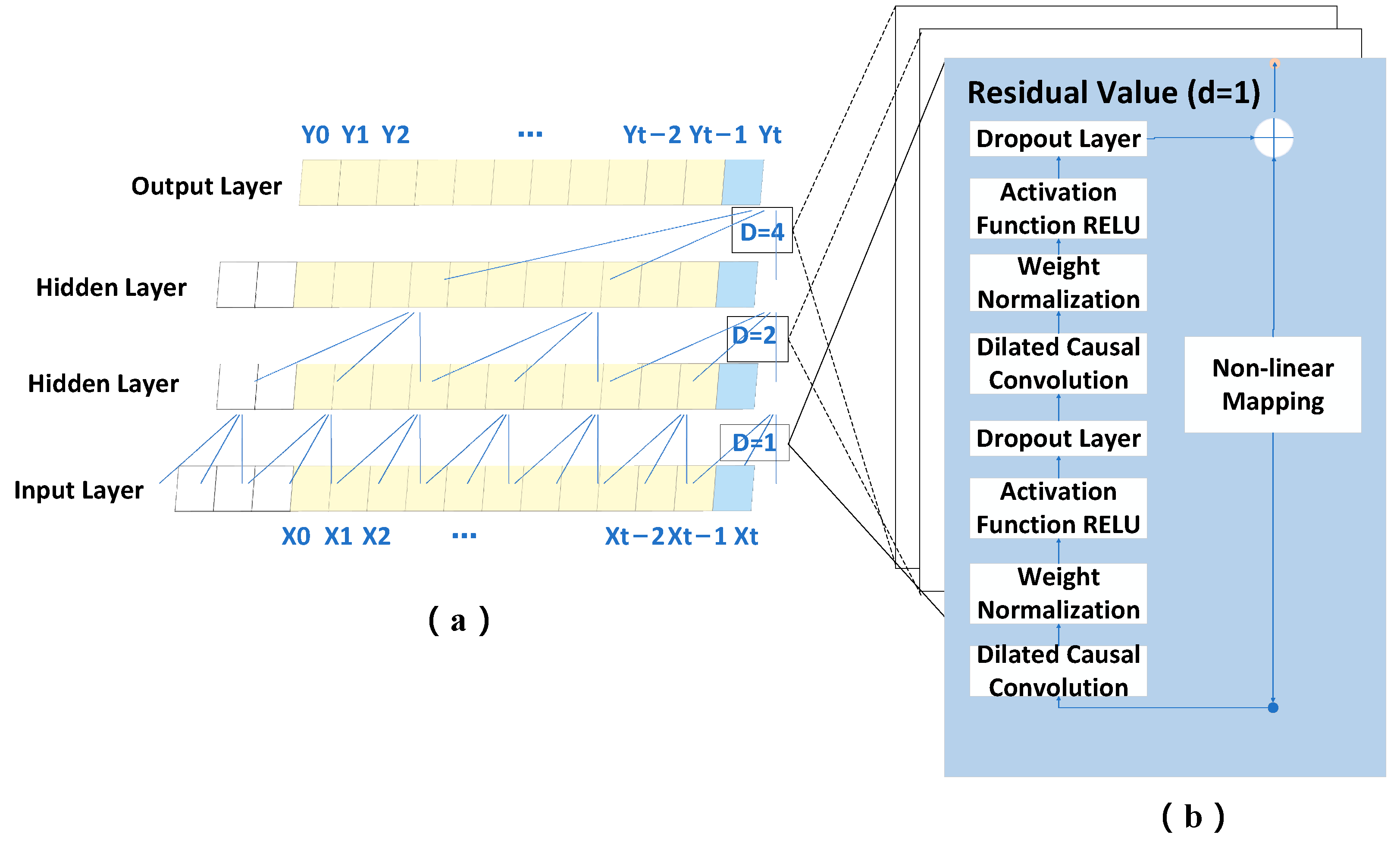
Figure 5 depicts the causal convolution and dilated convolution structures of the TCN. Among them, subgraph (a) shows the overall structure of TCN, the subgraph (b) represents the causal convolution within a single residual block. Causal convolution ensures the integrity of the input trajectory sequences, ensuring that the prediction value at moment t + 1 is only associated with the values of the previous t moments. On the other hand, dilated convolution allows the TCN to achieve a broader receptive field with fewer layers. The filters of dilated convolution can process input data in jumps, enabling the capture of input information farther from the current step. This approach enables the model to accommodate longer trajectory sequence data and effectively tackle the issue of long-distance dependencies in trajectory sequence data. At the same time, this paper employs the RELU activation function, dropout, and an identity mapping network to assist the model in learning more complex patterns and preventing neural network overfitting, resolving the issues of gradient vanishing and exploding in neural networks. Consequently, these implementations render the network more adept at deep learning, accelerating training speed and boosting the accuracy of trajectory predictions.
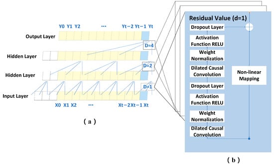
Figure 5.
TCN model.
Specifically, assume the model input represents a one-dimensional dilated causal convolution kernel; then the result after the dilated causal convolution operation is expressed as follows:
where d is the dilation rate; k is the kernel size; and represents the position point corresponding to the input sequence. When using dilated convolution, d usually increases exponentially with the depth of the network layer i specifically as . This variation ensures that the receptive domain of the TCN expands rapidly when the convolutional kernel size k is changed. This allows the convolutional kernels at higher levels in the network to cover all valid inputs to the input track sequence, resulting in better fusion of information.
3.2.2. Attention Layer
The attention mechanism mainly plays the role of filtering out the most important information for the current task from a large amount of information and highlighting important features. Attention mechanisms are valuable in terminal airspace trajectory prediction. In 4D trajectory prediction, the flight data may include large changes, such as the sudden change of flight direction or the rapid rise or fall of the aircraft’s altitude. In these cases, the attention mechanism can help the model to pay more attention to these critical moments instead of focusing only on the recent flight data. In this paper, we introduce the attention mechanism to calculate the weights of the vectors output at different moments in the TCN network, which can effectively highlight the features that have a greater impact on the predicted value of the trajectory.
The data are extracted by the TCN network and output T, is the number t feature vector output by the TCN network. We input it into the attention layer to get the initial state vector dt, and then give it the weight coefficient to get the final output state vector Y. The specific calculation process is as follows:
where represents the energy value corresponding to ; and represent the weight coefficient and bias corresponding to the number t eigenvector, respectively.
3.2.3. Trajectory Prediction Decoder GRU
Currently, seq2seq models mostly use RNN or LSTM as the encoder or decoder, but RNN has problems with, for example, gradient vanishing. GRU and LSTM are two derivatives of RNN, both of which are designed to solve the problems of gradient vanishing and exploding in traditional recurrent neural networks, but the GRU network is simpler and runs more efficiently than the LSTM network.
The GRU continuously updates information through its gated recurrent units. It integrates the forget gate and input gate into a single update gate, eliminating the need for a separate memory gate unit. By using the reset gate unit, the GRU simultaneously achieves both “selective forgetting” and “selective remembering” functionalities. This design effectively reduces the number of parameters in the network units, shortens the model training time, and mitigates the issues of gradient vanishing and exploding.
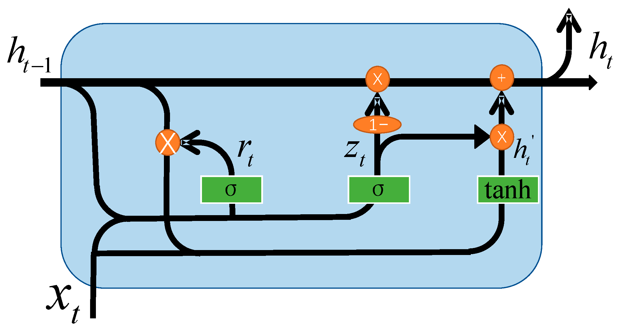
In the 4D trajectory prediction task within the terminal airspace, the GRU serves as the decoder to sequentially output a trajectory prediction sequence over n steps. Figure 6 illustrates the fundamental decoding process, where the decoder receives intermediate vectors processed by the attention mechanism. Each subsequent GRU unit takes in the current input and the previous hidden state, recursively generating GRU outputs until the complete trajectory sequence is generated.
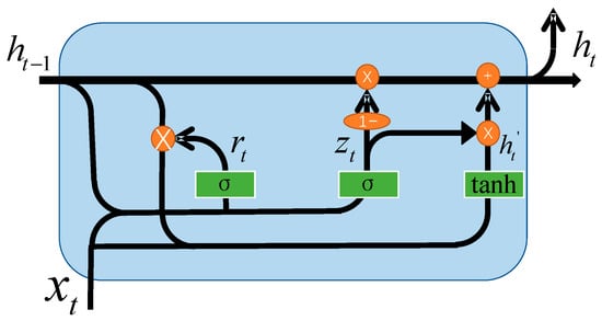
Figure 6.
GRU model.
Training Process Description: As depicted in Figure 6, the key components of the GRU network are the update gate and reset gate. The essential features during model training include the current input , the state vector of the previous moment , the state vector of the current moment , the candidate state vector of the current moment , the state vector of the update gate , and the state vector of the reset gate . The internal computation process is as follows:
where , , denote the parameter matrices to be learned; denotes the sigmoid function, whose function is to transform the input value into a value in the range of (0, 1) and then use this value as a gating signal. The main purpose of the hyperbolic tangent function (tanh) is to transform the input value into a value in the range (−1, 1).
3.2.4. Model Training
The purpose of model training is to reduce the level of error between predicted trajectories and actual trajectories. While the seq2seq framework is primarily used for text translation problems, considering the distinct nature of trajectory prediction, the model’s cost function has been modified to mean square error from posterior probability. The Adam optimizer is employed for parameter optimization. The detailed training process is as follows:
Firstly, we prepare the dataset by using the Spat Fill method to reconstruct the trajectory data, resulting in high-quality trajectory data that serve as our input. Next, we make initial parameter selections for the model. This includes determining the lengths of the input and output sequences, specifying the number of layers in the encoding and decoding networks, setting the number of neurons, defining the batch size, specifying the number of epochs, setting the stop criterion threshold, and establishing the initial learning rate. The lengths of the encoding and decoding sequences are determined based on the actual trajectory prediction task, while we optimize the other parameters within certain ranges. Following that, we train the model based on the loss function until predefined thresholds are met or until the training process reaches the specified number of epochs. Finally, we perform validation using a validation dataset. We input this dataset into the trajectory prediction model trained with the corresponding training data, conducting evaluation and fine-tuning.
4. Experimentation
4.1. Experimental Setup
Table 1 and Table 2 describe the specific settings and hyperparameters for implementing the 4D flight trajectory prediction model based on Attention-TCN-GRU. We use a grid search to determine the relevant parameters and use MSE as the loss function; the relevant parameter ranges are shown in Table 3. The experimental environment is run on the TensorFlow framework (developed by Google, Mountain View, CA, USA) for Windows and uses a GTX3060 GPU (manufactured by NVIDIA Corporation, Santa Clara, CA, USA) to accelerate the computation. The dataset used for the experiments has a total of 4049 take-off and landing trajectory sequences. For take-off and landing trajectories, the trajectories under abnormal conditions with excessive time were deleted, and then all other trajectories were populated with final state point data based on the longest trajectory in the normal range among the remaining normal trajectories. For the selected take-off and landing trajectories within the terminal area, it was found that the take-off time was around 200 s and the landing time was around 800 s. We set the input sequence lengths for take-off and landing to 50 s and 200 s respectively, while the output sequence covers the remaining lengths. During the prediction phase, we truncate the final continuous unaltered state points and retain only the first two repeated points, ensuring that our high-precision predictions align with the actual lengths of flight trajectories in civil aviation.

Table 1.
Setting of landing trajectory parameters.
Table 2.
Setting of take-off trajectory parameters.
Table 3.
Range of parameter choices for the model.
4.2. Test Indicators
In the Attention-TCN-GRU model, we evaluate the performance of the trajectory prediction model using two common metrics: root mean square error (RMSE) and mean absolute error (MAE). A lower value of these metrics indicates higher precision of the model in handling experimental data. The RMSE is calculated as the square root of the average of the squares of the differences between the predicted and observed values, serving as a measure of the average magnitude of errors. The MAE is the average of the absolute errors between the predicted and observed values, providing a more accurate representation of the true prediction error. We employ these two metrics to assess the effectiveness of Attention-TCN-GRU, with calculation methods as follows:
where denotes the real trajectory and denotes the predicted trajectory at moment i. In order to be able to fully test the performance of the Attention-TCN-GRU model, the prediction results of Attention-TCN-GRU are subsequently compared with a single LSTM network and SS-DLSTM.
4.3. Forecast Results and Comparative Analysis
The main aspects of the analysis are the prediction of busyness divisions, model complexity, comparative analysis, and comparison of assessment error values.
4.3.1. Assessment of Forecasting Results for Busyness Classification
For the processed take-off and landing dataset, we initially divide it into two categories based on take-offs and landings. We then identify busy periods during the operational dates of the flights and divide the take-off and landing datasets into busy and idle trajectory periods. This study extracts the data of all operating flights within a single day, from 0:00 to 24:00, and segments it into intervals of two hours each. Figure 7 illustrates the number of flights during each interval for both take-offs and landings. For departing flights, we define the busy period as 6:00 to 22:00. For arriving flights, we define the busy period as 8:00 to 0:00. We finally divide each of the partitioned datasets into a training set, a testing set, and a validation set in the ratio of 7:2:1.
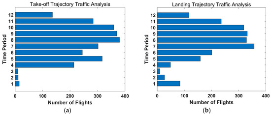
Figure 7.
Analysis of Track Business. (a) Take-off trajectory; (b) landing trajectory.
This study trains the designed Attention-TCN-GRU model on two sets of data: one that distinguishes between levels of busyness and another that does not. This process yields two distinct predictive models, each offering unique insights into flight operations. We subject both models to evaluations using an identical test set to ensure a uniform basis for performance comparison, with the detailed results presented in Table 4.
Table 4.
Error Evaluation of Busyness Index.
As shown in the above table, the prediction error of the prediction model trained by grouping the trajectory data using the busyness index is significantly lower than that of the prediction model without the busyness index. In addition, in order to facilitate a unified evaluation of the overall latitude, longitude, and altitude, we calculated the relative errors in the three dimensions. The latitude, longitude, and altitude errors using the busyness index were 1.01%, 3.09%, and 1.78%, respectively, while the latitude, longitude, and altitude errors without the busyness index were 1.58%, 3.61%, and 2.12%, respectively. It can be seen that grouping the levels of busyness has improved the prediction accuracy in all three dimensions to a certain extent. The landing and take-off trajectories grouped according to busyness can avoid the mutual interference between the busy time trajectories and the idle time trajectories, so that the model in each time period only learns the trajectory operation mode in the corresponding time period and realizes more accurate 4D trajectory predictions in the terminal area. The model that incorporates the busyness index predicts latitude, longitude, altitude, and time with lower errors and achieves a level of accuracy that meets the TBO requirements. Consequently, the Attention-TCN-GRU model, with the integrated busyness index, demonstrates enhanced predictive performance, boasting higher accuracy in predicting 4D trajectories within the terminal area.
4.3.2. Model Complexity Analysis
Firstly, we provide parameter settings for Attention-TCN-GRU models, SS-LSTM, and LSTM models. The Attention-TCN-GRU model’s parameter settings for take-off and landing phases are depicted in Table 2 and Table 3. The SS-LSTM model’s parameter complexity is essentially similar to the Attention-TCN-GRU model since both employ seq2seq architecture. This similarity extends to configurations such as the sliding window, learning rate, and batch size. Both models employ LSTM for their encoders and decoders, with the number of hidden layers for encoding take-off and landing trajectories being 3 and 4 respectively, and the neuron counts in each layer being (250, 150, 120) for take-off and (250, 150, 120, 100) for landing, both with a learning rate set to 0.001. In contrast, the LSTM model uses three hidden layers for both take-off and landing trajectories, each containing 128 units, with a batch size of 32 and a learning rate of 0.001. From the standpoint of parameter setting complexity, the Attention-TCN-GRU and SS-LSTM models exhibit a similar level of complexity, while the LSTM model is relatively simpler. A definitive assessment of model training performance, however, would require a consideration of training time.
By analysing the training time complexity of the designed model and evaluating its training time with a single LSTM model as well as the SS-DLSTM model for a given input size, it can help to understand the efficiency of the model when dealing with large-scale data. In this case, LSTM is a deep-learning model that incorporates space-time context for trajectory point prediction, whereas SS-DLSTM based on a seq2seq framework uses LSTM as a codec to predict the trajectory.
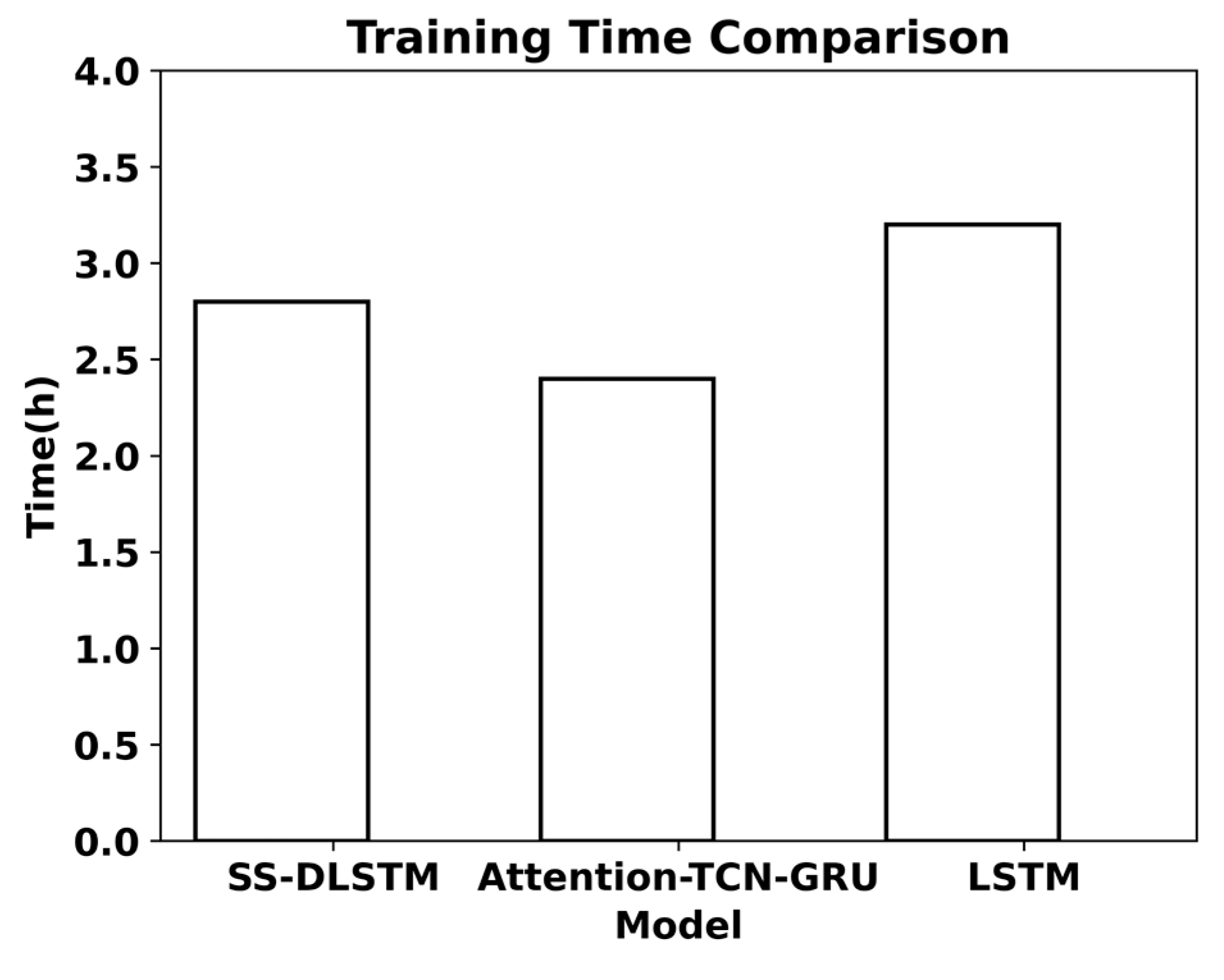
The time required for model training is reduced and it can bring more benefits in practical applications. Figure 8 illustrates the difference in time required for the training of each model. Among them, Attention-TCN-GRU is more efficient than SS-LSTM, indicating that the use of TCN, which has better performance in capturing long sequences, and GRU, which has higher efficiency, as the decoder, and the introduction of the attention mechanism, can accelerate the convergence of the loss function and focus on the important trajectory points in the prediction of aircraft trajectories, and also greatly reduce the training cost compared with the basic LSTM model. Therefore, the complexity of the model is optimized under the condition of guaranteeing accuracy, and it is suitable for 4D trajectory prediction in the terminal area.

Figure 8.
Comparison of model training time.
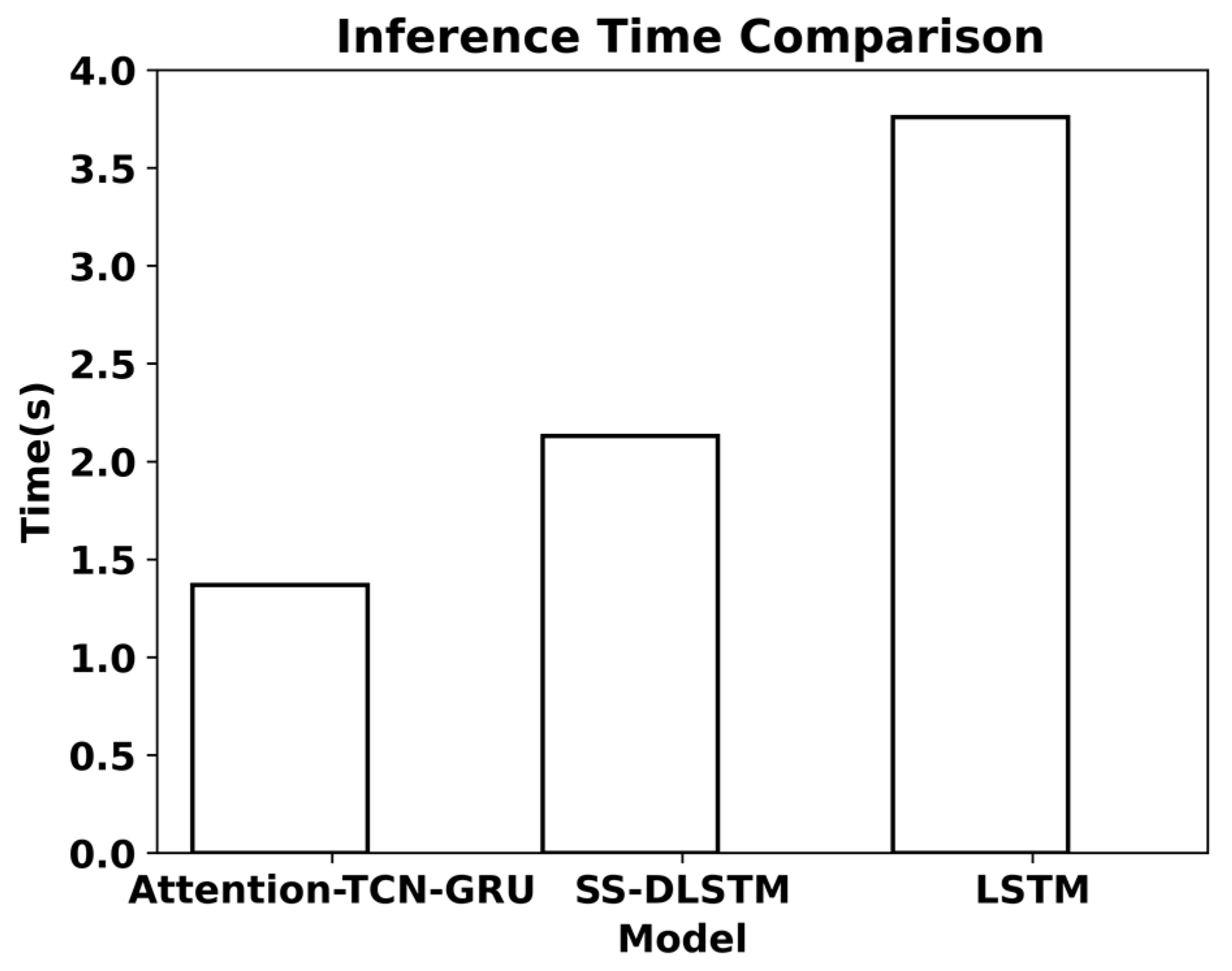
Additionally, as illustrated in Figure 9, we have also conducted statistics on the inference time of each model. It is evident from the figure that once trained, our designed model achieves the fastest inference speed in practical trajectory prediction tasks, approximately 1.5 s, which is fully capable of handling real-time trajectory prediction tasks.

Figure 9.
Comparison of model inference time.
4.3.3. Comparative Analysis of Models
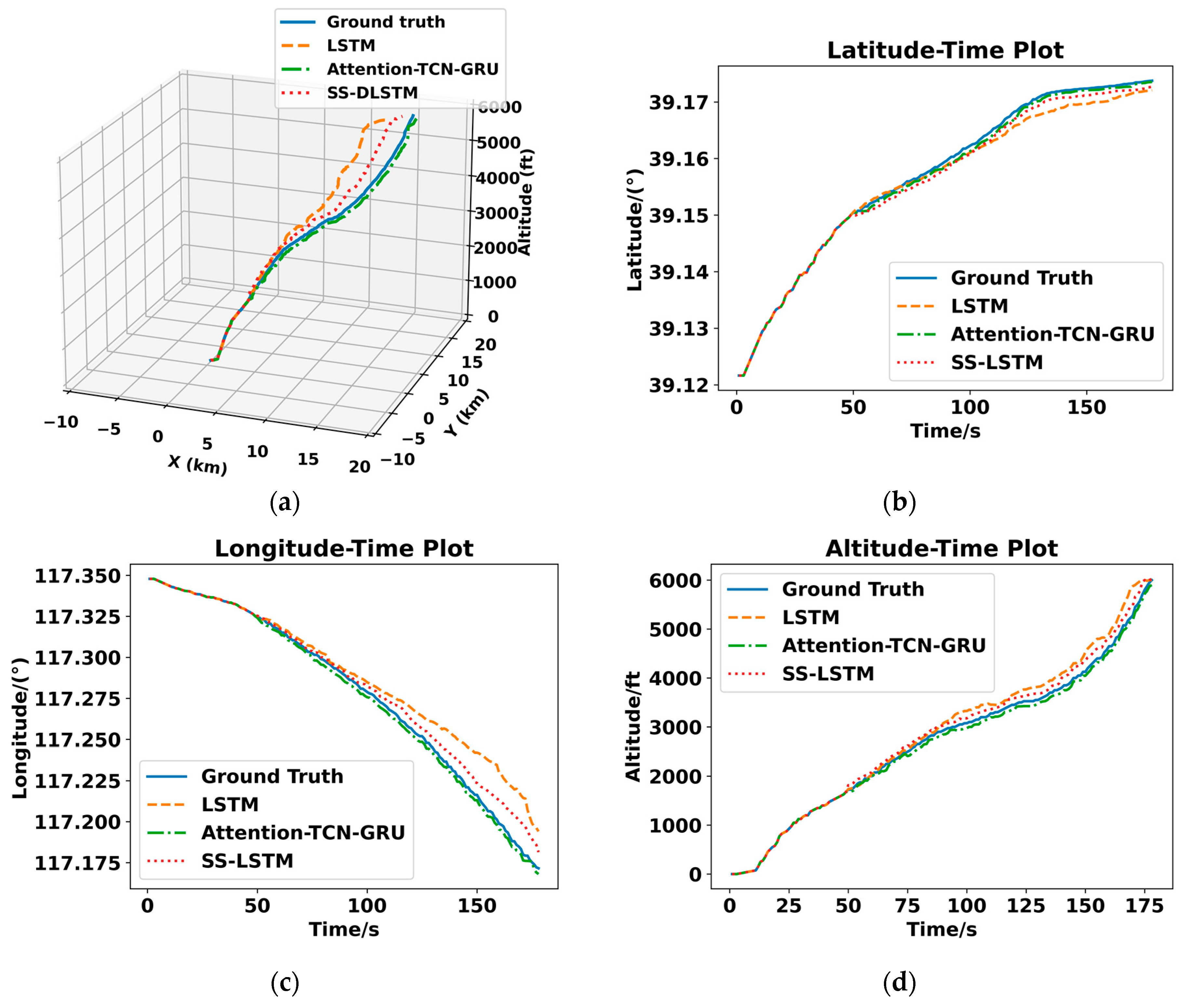
This study selects two representative predicted trajectories from the landing and take-off validation datasets following the incorporation of the busyness index. Figure 9 and Figure 10 visualize the predictive results of the flight take-off and landing trajectories, showcasing two-dimensional plots of predicted and actual paths over latitude-time, longitude-time, and altitude-time, along with a three-dimensional curve of latitude, longitude, and altitude. We only plot the coordinates that encompass the entire trajectory to clearly illustrate the discrepancies between the predicted and actual paths.
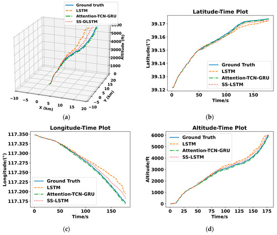
Figure 10.
Comparison of Prediction Results of Take-off Track Models. (a) Three-dimensional trajectories; (b) latitude-time two-dimensional trajectories; (c) longitude-time two-dimensional trajectories; (d) altitude-time two-dimensional trajectories.
Figure 10 and Figure 11a–d show the 3D comparison of the predicted trajectories with the real trajectories and the 2D comparison of latitude, longitude, and altitude over time from each model, respectively. It can be seen that, for the take-off trajectory, the overall trend of the three models is the same as that for the real trajectory, and the models basically fit the real trajectory well from the prediction point to the trajectory of 100 s. After that, the LSTM model shows a significant decrease, and the SS-DLSTM model also shows a decreasing trend, while the Attention-TCN-GRU model designed in this paper, which has better performance in dealing with long sequences, maintains the performance of prediction better, and its overall prediction accuracy is significantly higher than the other two models. It is well illustrated that the present algorithm can better meet the 4D trajectory prediction of terminal area departure.
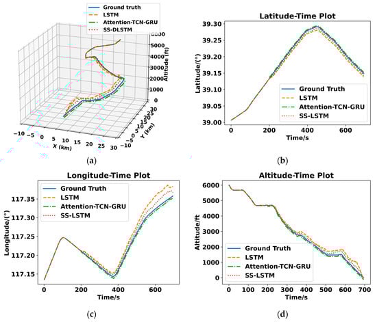
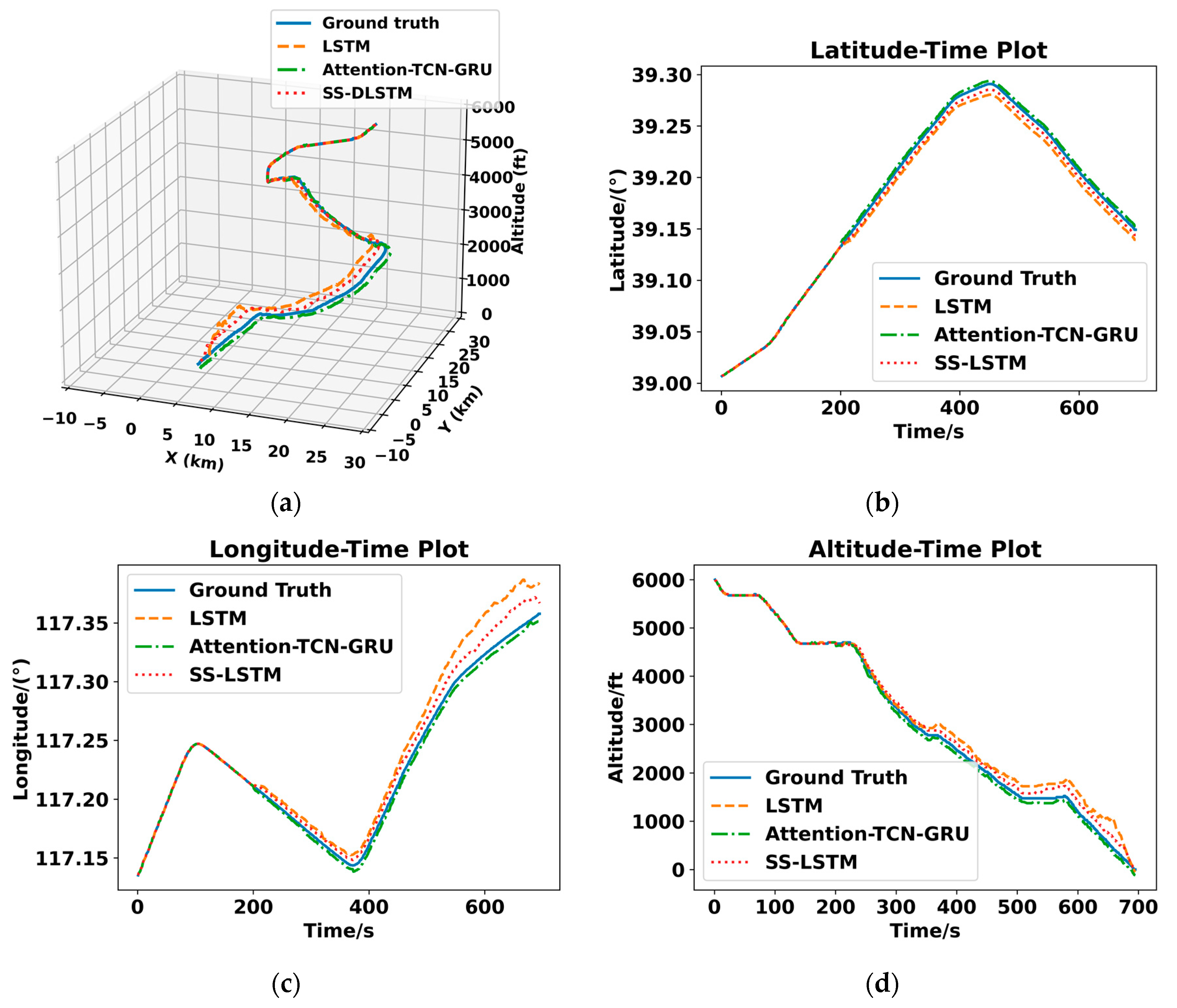
Figure 11.
Comparison of Prediction Results of Landing Track Models. (a) Three-dimensional trajectories; (b) latitude-time two-dimensional trajectories; (c) longitude-time two-dimensional trajectories; (d) altitude-time two-dimensional trajectories.
For the landing trajectories, all three models maintain predictions that are relatively consistent with the actual trajectories. In contrast to the prediction accuracy for take-off trajectories, the prediction accuracy for landing trajectories shows a slight decrease. This can be attributed to the fact that departing aircraft spend slightly less time in the terminal airspace and exhibit relatively fewer trajectory patterns, whereas landing aircraft trajectories are characterized by greater uncertainty and variability. Nevertheless, the Attention-TCN-GRU model continues to demonstrate strong predictive performance, indicating that the model designed in this study exhibits favourable advantages in predicting both take-off and landing trajectories within the terminal area. In summary, the latitude, longitude, and altitude over time prediction results of the three models are basically consistent with the actual trajectories. Compared with the other two models, the prediction curve of the LSTM model has a larger deviation from the actual trajectories. Compared with LSTM, the SS-DLSTM and Attention TCN-GRU models have smaller prediction errors for latitude, longitude, and altitude, indicating that the seq2seq framework is more suitable for 4D trajectory prediction in the terminal area than the single neural network LSTM. The Attention-TCN-GRU model has the best prediction accuracy, which indicates that the use of a TCN with strong long-sequence processing ability as the encoder for terminal area track predictions, the inclusion of the attention mechanism, and the use of the more efficient GRU as the decoder can improve the prediction accuracy of the 4D track in the terminal area. Indeed, the designed Attention-TCN-GRU model outperforms existing terminal area trajectory prediction models, showcasing superior predictive performance in terminal area trajectory prediction.
4.3.4. Comparison of Assessment Error Values
By comparing the predicted trajectories with the actual trajectories, we obtained the values of the RMSE and MAE as evaluation metrics. This study calculated the prediction errors of the models for latitude, longitude, altitude, and time in the terminal area 4D trajectories, along with the average errors for each model. The results are summarized in Table 5.
Table 5.
Model error evaluation.
According to the above table, the prediction error of Attention-TCN-GRU model is smaller than that of both SS-DLSTM and LSTM. In addition, due to the significant difference in numerical accuracy between the latitude and longitude provided by the global navigation satellite system and the altitude provided by the barometric altimeter in the input data, the expression of absolute values cannot accurately express the relationship between the altitude prediction error and the two-dimensional latitude and longitude errors. Therefore, we calculated the relative values at three latitudes, using the ratio of the difference between the predicted value and the true value to the true value. For latitude and longitude, we establish a coordinate axis based on the centre of the airport to redefine the corresponding latitude and longitude coordinates for the waypoint, instead of directly using the latitude and longitude coordinates under the Earth coordinate axis, to avoid the problem of large differences between the erroneous latitude and longitude and the actual latitude and longitude, which cannot demonstrate the predictive performance through relative value errors. The latitude, longitude, and altitude errors of Attention TCN-GRU after calculation are 1.01%, 3.09%, and 1.78%, respectively. The latitude, longitude, and altitude errors of SS-LSTM are 2.05%, 4.51%, and 2.88%, respectively. The latitude, longitude, and altitude errors of LSTM are 2.51%, 9.44%, and 4.01%, respectively. The total root mean square error of Attention-TCN-GRU model is 55.97% lower than that of the LSTM model and 32.07% lower than that of the SS-DLSTM model.
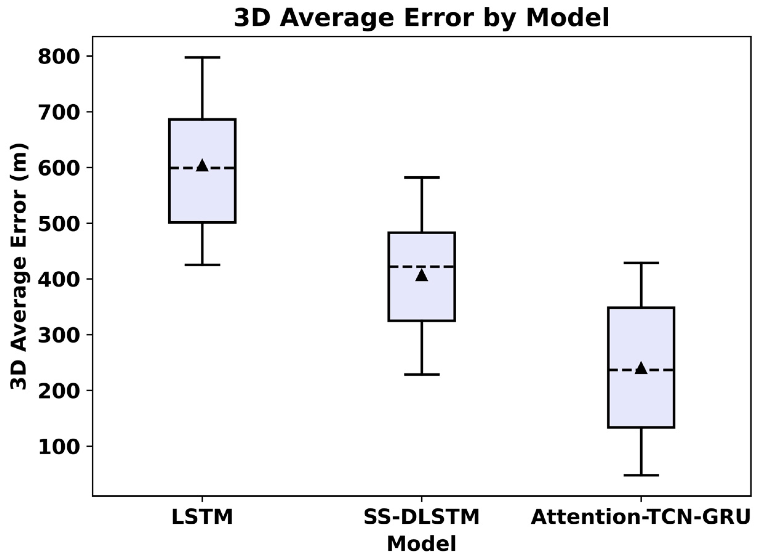
In addition, as shown in Figure 12, we averaged the latitude, longitude, and altitude of the three models’ take-off and landing trajectories to obtain a composite evaluation metric, and then implemented a box-and-line plot analysis of the three models. It is also clear in the figure that the median and mean prediction errors of the Attention-TCN- GRU model are around 250m, and the SS-LSTM and LSTM are around 420 and 600, respectively, which fully meets the requirements for trajectory prediction in terms of accuracy and illustrates that the Attention-TCN-GRU model achieves more accurate predictions and is a more suitable model for 4D trajectory predictions in terminal airspace.
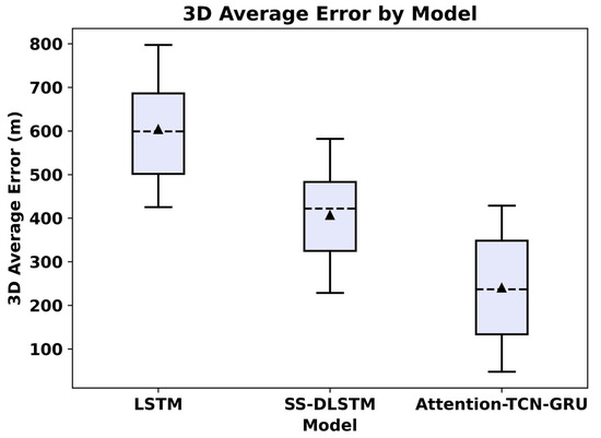
Figure 12.
Comparative analysis of model boxplots.
Additionally, by converting the data from Table 2, the latitude error is found to be about 244.9 m, the longitude error about 1135.5 m, and the altitude error around 40.0 m. According to regulations set by the Civil Aviation Authority, the operational track horizontal separation in the terminal area is 6000 m and the vertical separation is 300 m. The prediction errors in both the horizontal and vertical directions proposed in this article are lower than the relevant errors. Therefore, the trajectory prediction model in this paper has the potential to provide basic technical support for conflict detection methods in the aviation industry. However, there is still room for improvement in high-level safe and efficient conflict detection.
5. Conclusions
This paper addresses the terminal airspace around airports and presents a data-driven aircraft trajectory prediction model based on an extensive dataset of ADS-B historical flight tracks. Initially, the Spat Fill method is employed to reconstruct equally spaced high-quality flight tracks as the initial inputs for the prediction model. Subsequently, we frame trajectory prediction as a problem in which historical flight track sequences are mapped to future flight track sequences. Building upon seq2seq theory, we propose an Attention-TCN-GRU model. This model leverages TCN as an encoder for better handling of long sequences, employs the efficient GRU as a decoder, and integrates attention mechanisms to enhance the learning of temporal correlations within flight track sequences. Using aircraft trajectory features such as latitude, longitude, altitude, heading, and speed as inputs, the model recursively generates latitude, longitude, and altitude information for future flight track sequences over time. We applied the proposed model to a dataset from a major domestic airport’s terminal airspace, and the study revealed that employing seq2seq theory in 4D trajectory prediction within the terminal airspace is highly effective. Furthermore, the predictive performance of the designed Attention-TCN-GRU model surpasses that of the current mainstream prediction models.
However, the incorporation of variables with significant impacts on flight paths, such as ANSP decisions and meteorological conditions, remains a challenge. In future data-driven 4D trajectory prediction research, we will consider factors such as ANSP decision, flight procedures, weather conditions, and aircraft intentions to enhance the predictive performance of our model. In addition, the generalization of the model is also a future research focus, considering terminal area trajectory data under multiple different structures for large validation in order to improve the establishment of terminal area trajectory prediction models with different structural types and achieve accurate predictions on a large scale. Finally, training the local QNH pressure feature set would enable the model to consider the impact of QNH on height values, improving height prediction accuracy, and this is also a future research goal.
Author Contributions
Conceptualization, L.M. and Z.W.; methodology, L.M., Z.W. and X.M.; Software, X.M.; Validation, X.M.; data curation, Z.W.; writing—original draft preparation, L.M. and X.M.; writing—review and editing, Z.W. and L.M.; Supervision, Z.W.; All authors have read and agreed to the published version of the manuscript.
Funding
This research was funded by National Natural Science Foundation of China (NSFC) and Civil Aviation Administration of China, grant number U1333116.
Data Availability Statement
The data used to support the findings of this study are available from the corresponding author upon request.
Conflicts of Interest
The authors declare no conflicts of interest.
References
- Chatterji, G. Short-term trajectory prediction methods, AIAA 1999-4233. In Proceedings of the Guidance, Navigation, and Control Conference and Exhibit, Portland, OR, USA, 9–11 August 1999. [Google Scholar]
- Gong, C.; McNally, D. A Methodology for Automated Trajectory Prediction Analysis, AIAA 2004-4788. In Proceedings of the AIAA Guidance, Navigation, and Control Conference and Exhibit, Providence, RI, USA, 16–19 August 2004. [Google Scholar]
- Lymperopoulos, I.; Lygeros, J.; Lecchini, A. Model Based Aircraft Trajectory Prediction during Takeoff, AIAA 2006-6098. In Proceedings of the AIAA Guidance, Navigation, and Control Conference and Exhibit, Keystone, CO, USA, 21–24 August 2006. [Google Scholar]
- Rentas, T.; Green, S.; Cate, K. Characterization Method for Determination of Trajectory Prediction Requirements, AIAA 2009-6989. In Proceedings of the 9th AIAA Aviation Technology, Integration, and Operations Conference (ATIO), Hilton Head, CA, USA, 21–23 September 2009. [Google Scholar]
- Mondoloni, S. A Multiple-Scale Model of Wind-Prediction Uncertainty and Application to Trajectory Prediction, AIAA 2006-7807. In Proceedings of the 6th AIAA Aviation Technology, Integration and Operations Conference (ATIO), Wichita, KS, USA, 25–27 September 2006. [Google Scholar]
- Klooster, J.; Wichman, K.; Bleeker, O. 4D Trajectory and Time-of-Arrival Control to Enable Continuous Descent Arrivals, AIAA 2008-7402. In Proceedings of the AIAA Guidance, Navigation and Control Conference and Exhibit, Honolulu, HI, USA, 18–21 August 2008. [Google Scholar]
- de Leege, A.; van Paassen, M.; Mulder, M. A Machine Learning Approach to Trajectory Prediction, AIAA 2013-4782. In Proceedings of the AIAA Guidance, Navigation, and Control (GNC) Conference, Boston, MA, USA, 19–22 August 2013. [Google Scholar]
- Le Fablec, Y.; Alliot, J.-M. Using neural networks to predict aircraft trajectories. In Proceedings of the IC-AI, Las Vegas, NV, USA, 28 June–1 July 1999. [Google Scholar]
- Thipphavong, D.P.; Schultz, C.A.; Lee, A.G.; Chan, S.H. Adaptive Algorithm to Improve Trajectory Prediction Accuracy of Climbing Aircraft. J. Guid. Control. Dyn. 2013, 36, 15–24. [Google Scholar] [CrossRef]
- Han, Y.; Tang, X.; Han, S. Conflict-free 4D trajectory prediction based on hybrid system theory. J. Southwest Jiaotong Univ. 2012, 47, 1069–1074. [Google Scholar]
- Liu, W.; Hwang, I. Probabilistic trajectory prediction and conflict detection for air traffic control. J. Guid. Control. Dyn. 2011, 34, 1779–1789. [Google Scholar] [CrossRef]
- Ayhan, S.; Samet, H. Aircraft trajectory prediction made easy with predictive analytics. In Proceedings of the 22nd ACM SIGKDD International Conference on Knowledge Discovery and Data Mining, San Francisco, CA, USA, 13–17 August 2016; pp. 21–30. [Google Scholar]
- Wang, Z.; Liang, M.; Delahaye, D. Short-Term 4d Trajectory Prediction Using Machine Learning Methods. In Proceedings of the SESAR Innovation Day SID, Belgrade, Serbia, 28–30 November 2017. [Google Scholar]
- Hernández, A.M.; Magaña, E.J.C.; Berná, A. Data-driven aircraft trajectory predictions using ensemble meta-estimators. In Proceedings of the 2018 IEEE/AIAA 37th Digital Avionics Systems Conference (DASC), London, UK, 23–27 September 2018; IEEE: New York, NY, USA, 2018; pp. 1–10. [Google Scholar]
- Barratt, S.T.; Kochenderfer, M.J.; Boyd, S.P. Learning probabilistic trajectory models of aircraft in terminal airspace from position data. IEEE Trans. Intell. Transp. Syst. 2018, 20, 3536–3545. [Google Scholar] [CrossRef]
- Hong, S.; Lee, K. Trajectory prediction for vectored area navigation arrivals. J. Aerosp. Inf. Syst. 2015, 12, 490–502. [Google Scholar] [CrossRef]
- Alligier, R.; Gianazza, D.; Durand, N. Machine learning and mass estimation methods for ground-based aircraft climb prediction. IEEE Trans. Intell. Transp. Syst. 2015, 16, 3138–3149. [Google Scholar] [CrossRef]
- Pang, Y.T.; Wang, Y.H.; Liu, Y.M. Probabilistic aircraft trajectory prediction with weather uncertainties using approximate Bayesian variational inference to neural networks. In Proceedings of the AIAA Aviation 2020 Forum, Virtual Event, 15–19 June 2020. [Google Scholar]
- Shi, Z.Y.; Xu, M.; Pan, Q. 4-D flight trajectory prediction with constrained LSTM network. IEEE Trans. Intell. Transp. Syst. 2021, 22, 7242–7255. [Google Scholar] [CrossRef]
- Fan, Z.; Lu, J.; Qin, Z. Aircraft Trajectory Prediction Based on Residual Recurrent Neural Networks. In Proceedings of the 2023 IEEE 2nd International Conference on Electrical Engineering, Big Data and Algorithms (EEBDA), Changchun, China, 24–26 February 2023; pp. 1820–1824. [Google Scholar]
- Tran, P.N.; Nguyen, H.Q.V.; Pham, D.-T.; Alam, S. Aircraft Trajectory Prediction with Enriched Intent Using Encoder-Decoder Architecture. IEEE Access 2022, 10, 17881–17896. [Google Scholar] [CrossRef]
- Wang, X.; Wang, J.; Hou, J.; Song, M.; Xu, W.; Li, J. TraNet: A Hybrid Deep Neural Network for Long-Time-Scale Aircraft Trajectory Prediction International Conference on Guidance, Navigation and Control; Springer Nature: Singapore, 2022; pp. 4408–4419. [Google Scholar]
- Zeng, W.; Quan, Z.; Zhao, Z.; Xie, C.; Lu, X. A deep learning approach for aircraft trajectory prediction in terminal airspace. IEEE Access 2020, 8, 151250–151266. [Google Scholar] [CrossRef]
- Jun, L.Z.; Alam, S.; Dhief, I.; Schultz, M. Towards a greener Extended-Arrival Manager in air traffic control: A heuristic approach for dynamic speed control using machine-learned delay prediction model. J. Air Transp. Manag. 2022, 103, 102250. [Google Scholar] [CrossRef]
- Lui, G.N.; Klein, T.; Liem, R.P. Data-driven approach for aircraft arrival flow investigation at terminal maneuvering area. In Proceedings of the AIAA Aviation 2020 Forum, Virtual Event, 15–19 June 2020; p. 2869. [Google Scholar]
- Wandelt, S.; Sun, X.; Fricke, H. ADS-BI: Compressed Indexing of ADS-B Data. IEEE Trans. Intell. Transp. Syst. 2018, 19, 3795–3806. [Google Scholar] [CrossRef]
- Cho, K.; Van Merriënboer, B.; Gulcehre, C.; Bahdanau, D.; Bougares, F.; Schwenk, H.; Bengio, Y. Learning Phrase Representations using RNN Encoder–Decoder for Statistical Machine Translation. In Proceedings of the Conference on Empirical Methods in Natural Language Processing, Doha, Qatar, 25–29 October 2014. [Google Scholar]
- Fu, S.Q.; Li, Z.; Zhao, R.L.; Guo, J.X. Code Completion Approach Based on Combination of Syntax and Semantics. Ruan Jian Xue Bao J. Softw. 2022, 33, 3930–3943. Available online: http://www.jos.org.cn/1000-9825/6324.htm (accessed on 10 January 2024). (In Chinese).


Disclaimer/Publisher’s Note: The statements, opinions and data contained in all publications are solely those of the individual author(s) and contributor(s) and not of MDPI and/or the editor(s). MDPI and/or the editor(s) disclaim responsibility for any injury to people or property resulting from any ideas, methods, instructions or products referred to in the content. |
© 2024 by the authors. Licensee MDPI, Basel, Switzerland. This article is an open access article distributed under the terms and conditions of the Creative Commons Attribution (CC BY) license (https://creativecommons.org/licenses/by/4.0/).