
Determining the Location of the UAV When Flying in a Group


Abstract
1. Introduction
- Cooperative trajectory planning based on intelligent optimization algorithms
- Cooperative trajectory planning based on reinforcement learning
- Cooperative trajectory planning based on the spline interpolation algorithm
2. Materials and Methods
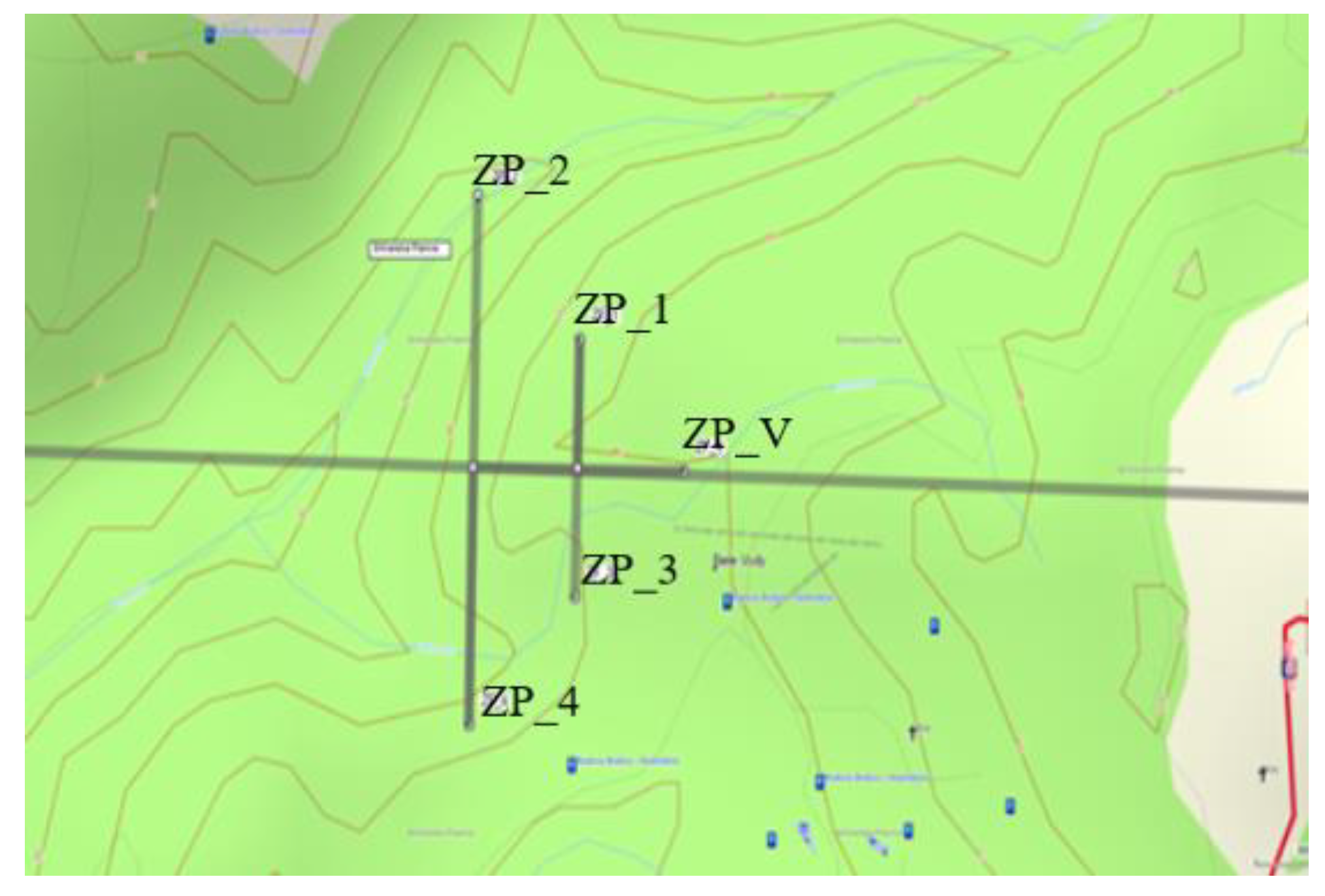
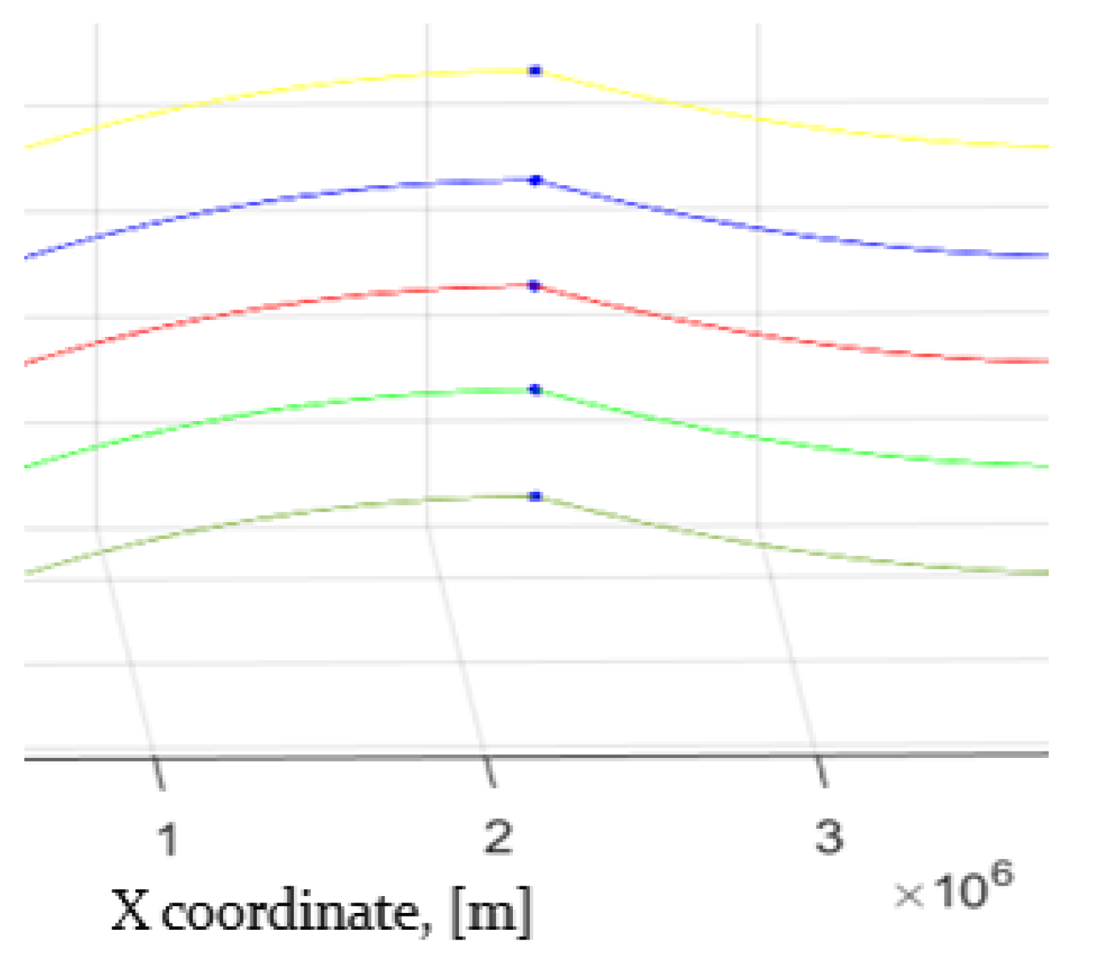
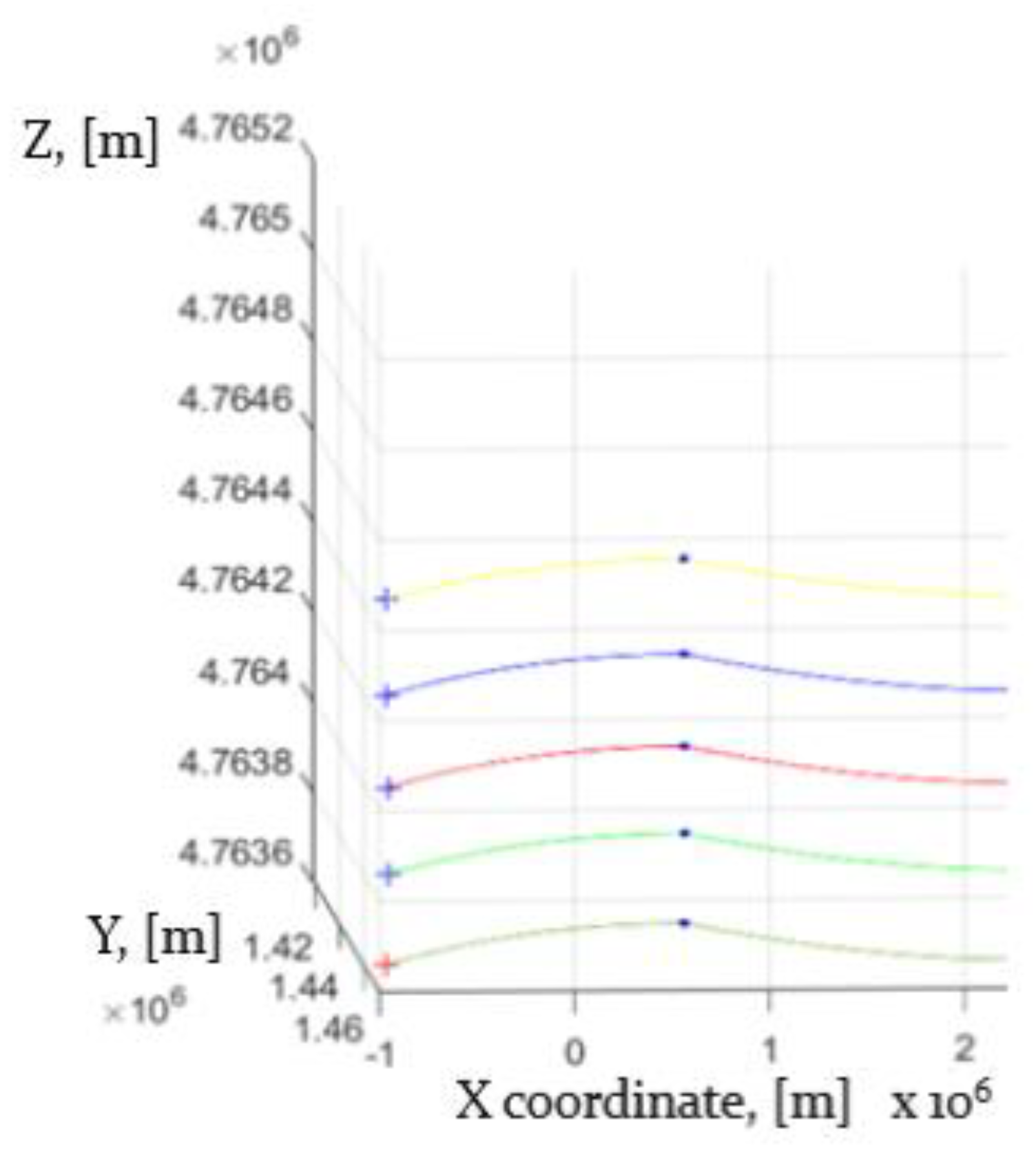
2.1. Flight Trajectory Model of a Group of Five UAVs
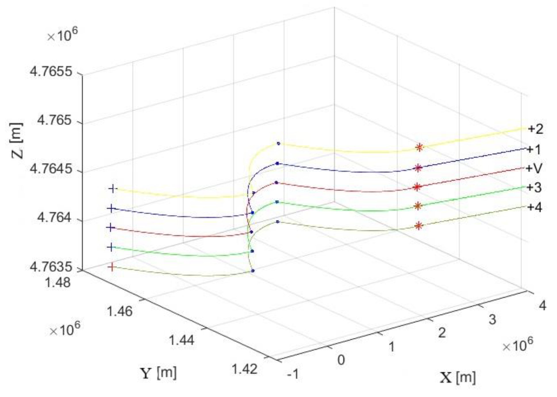
Simulation Results
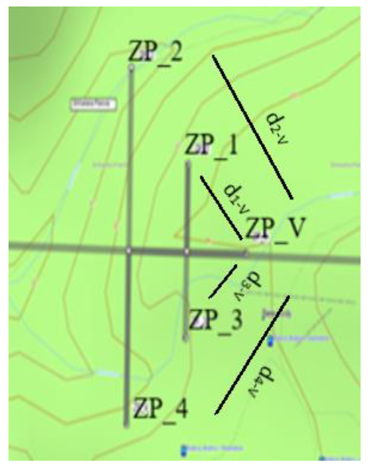
2.2. Model of the Communication Network of a Group of UAVs
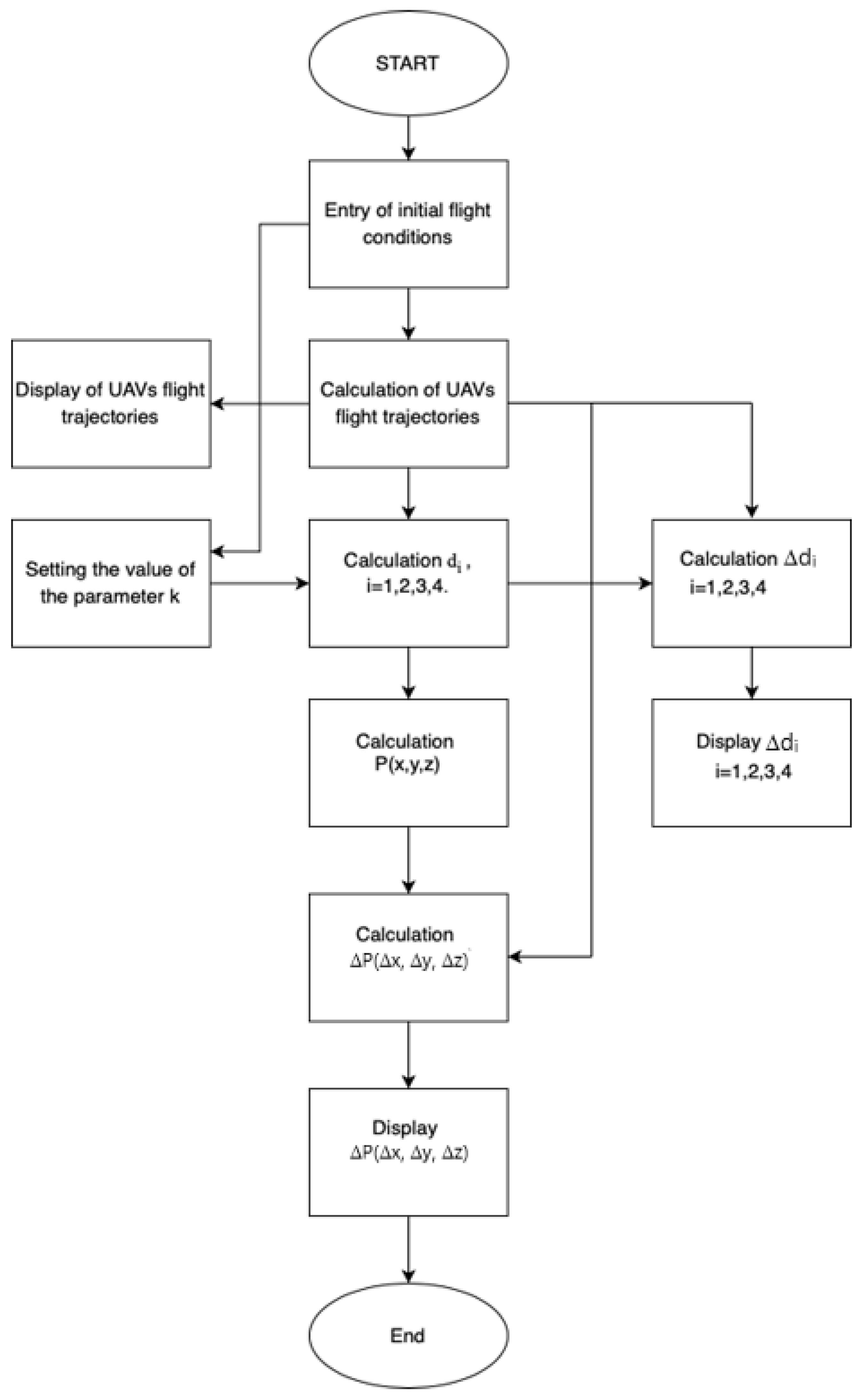
2.3. Equations for Determining the Location of a Selected Member of a Group of UAVs
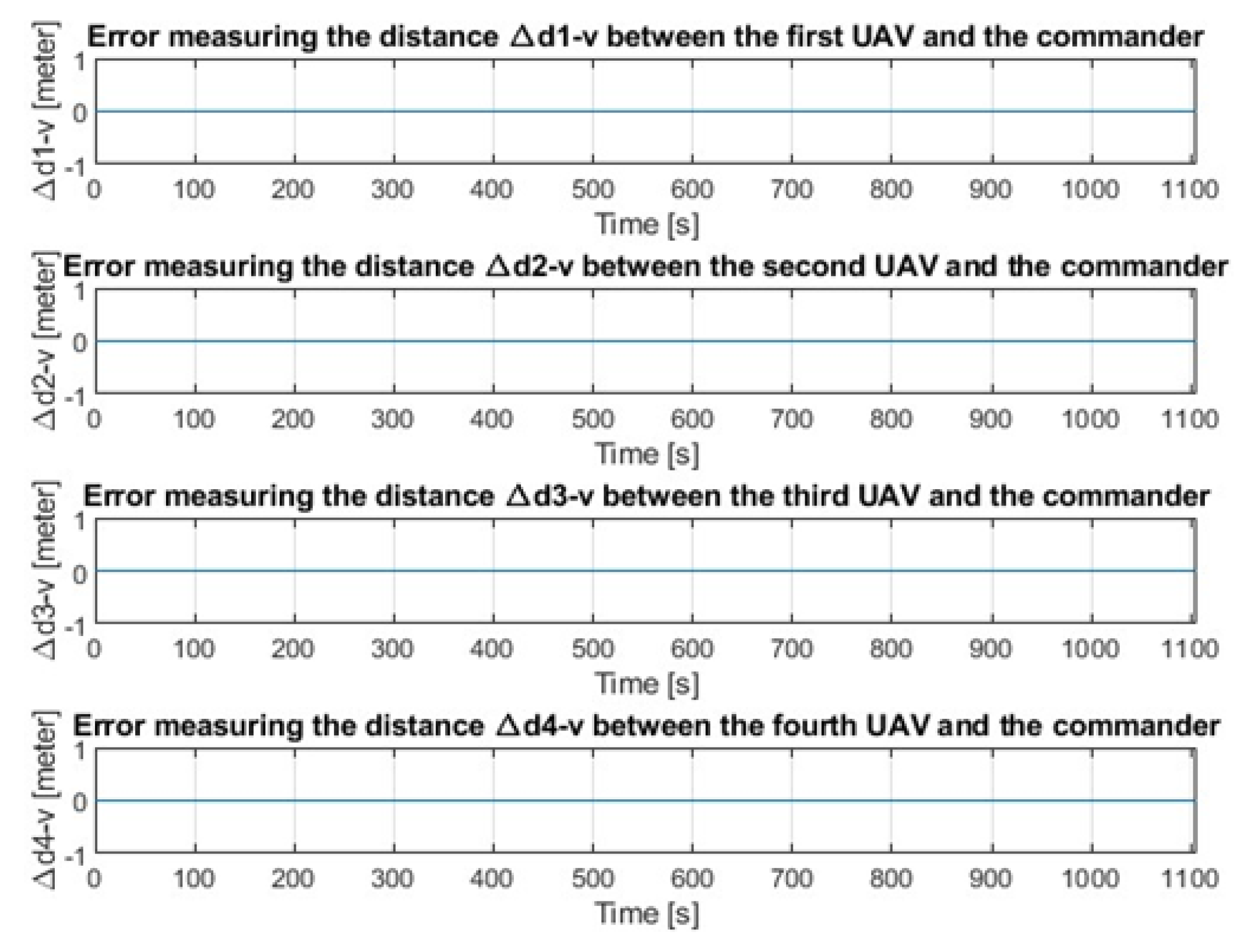
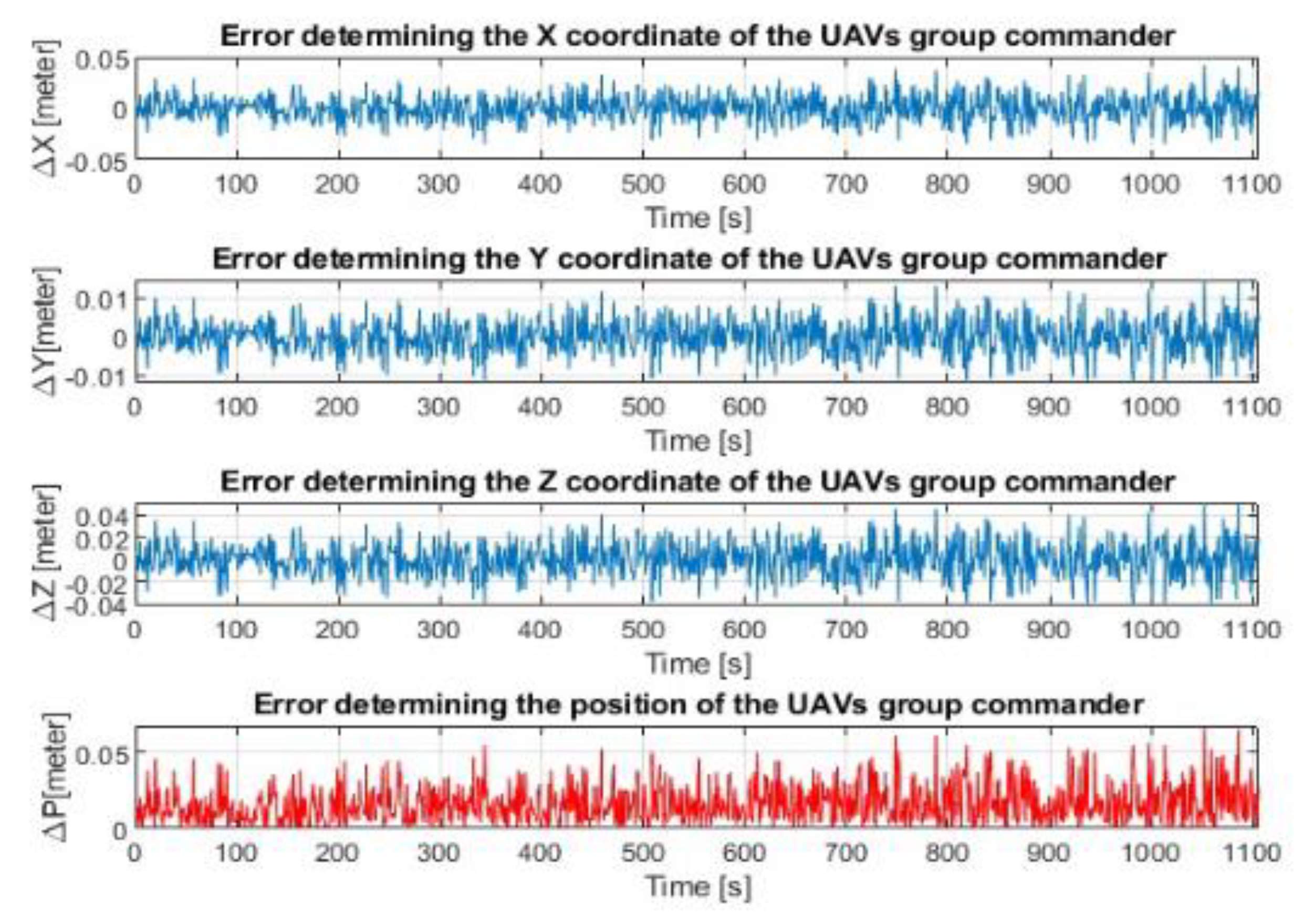
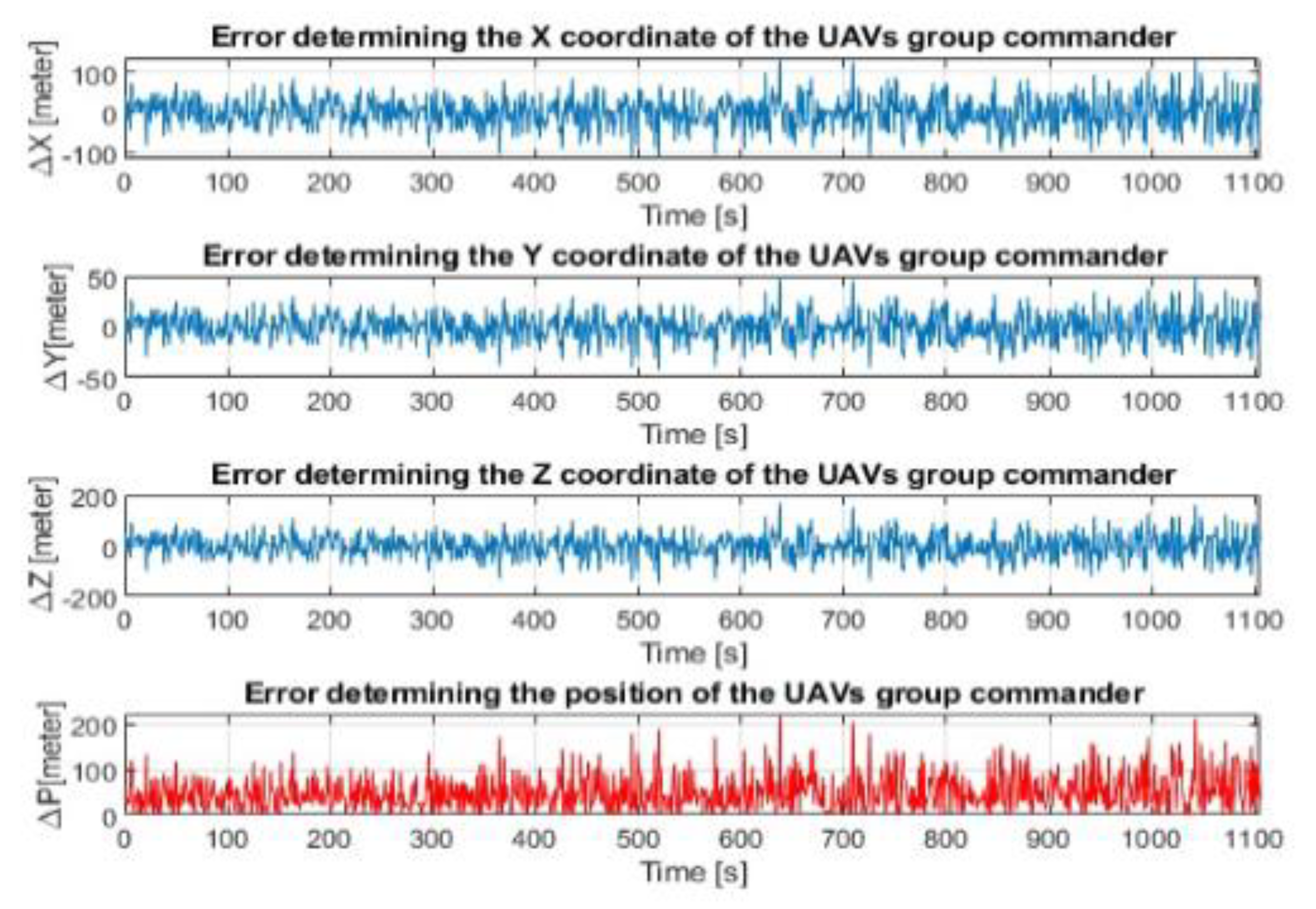
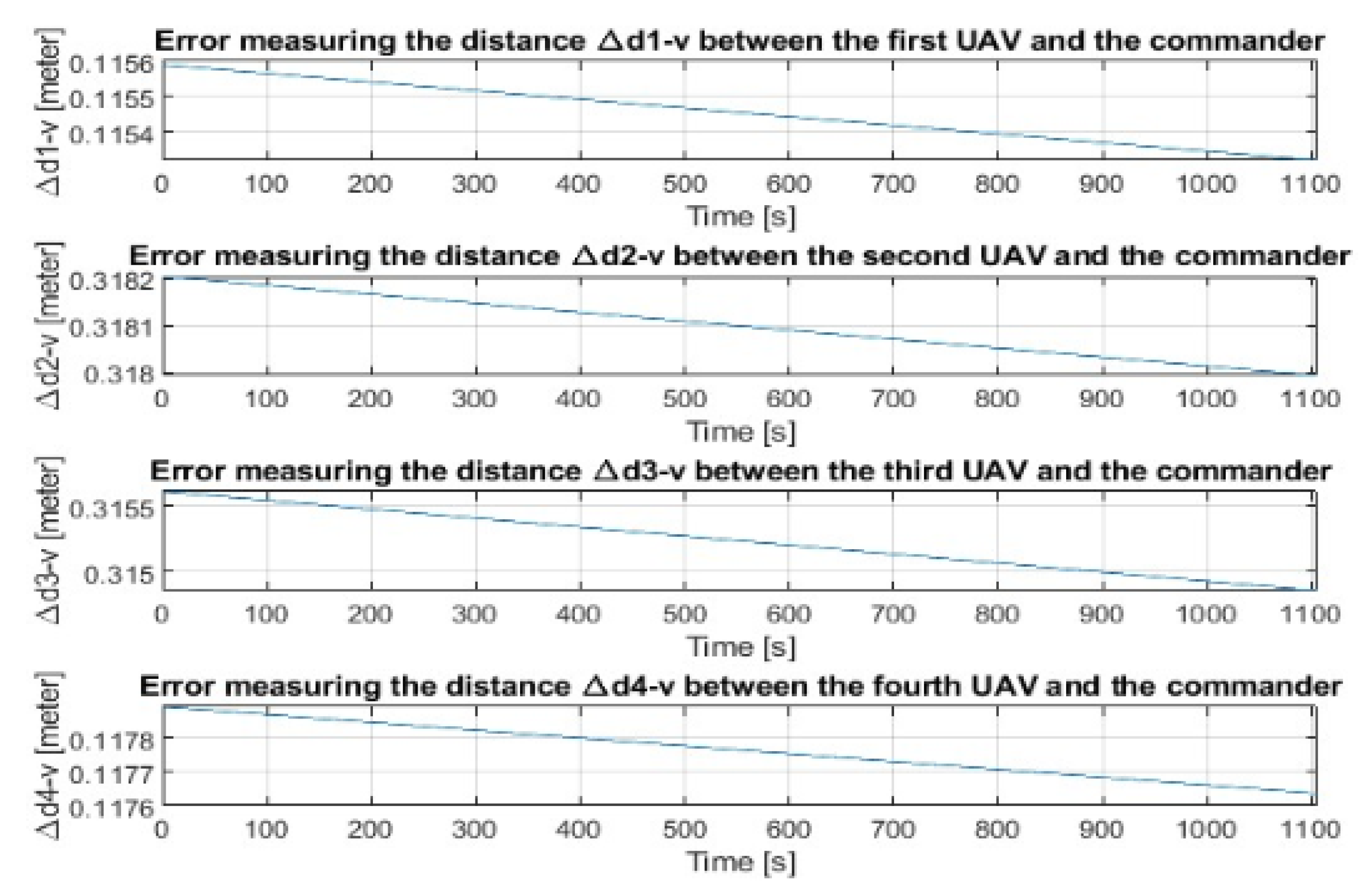
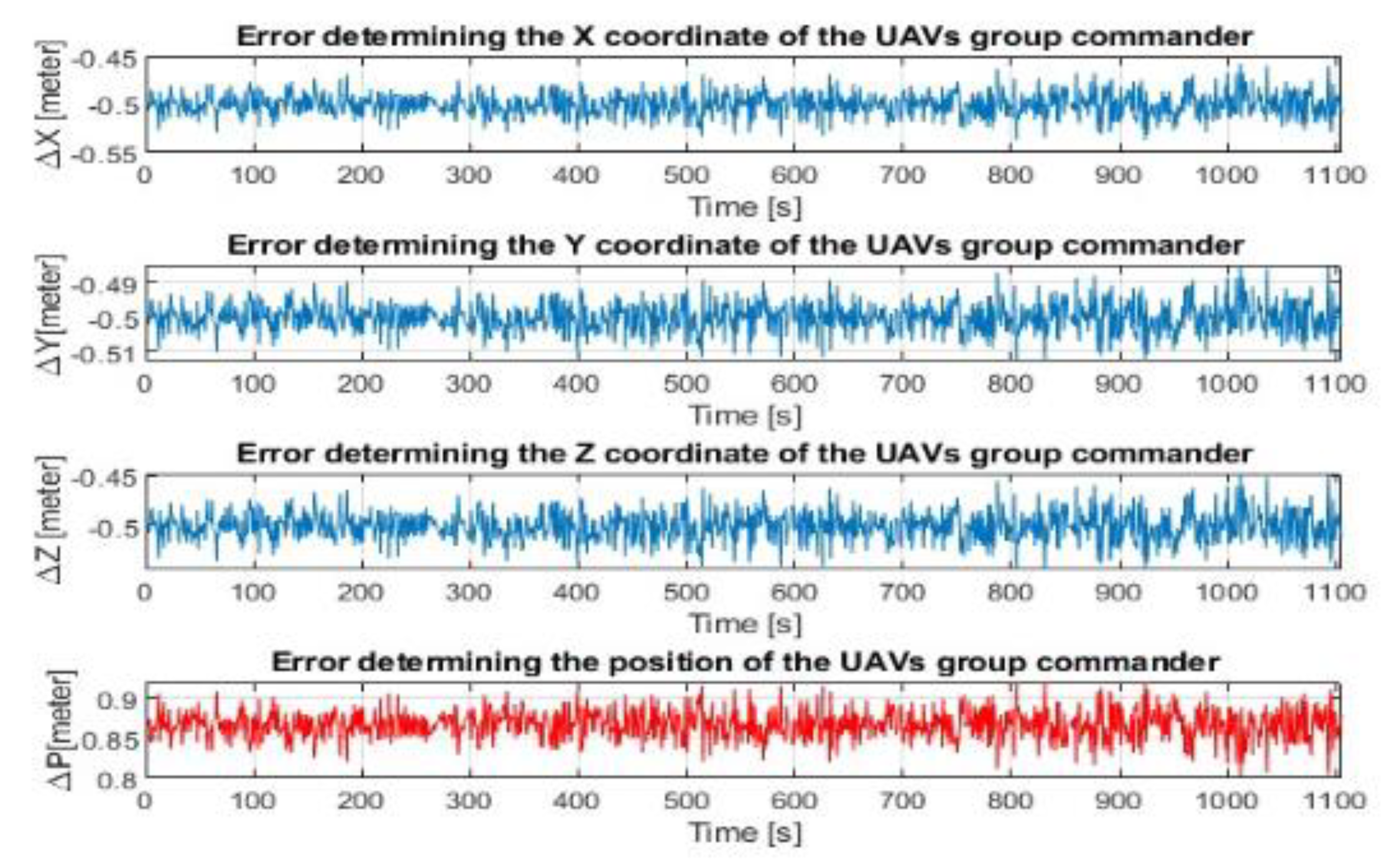
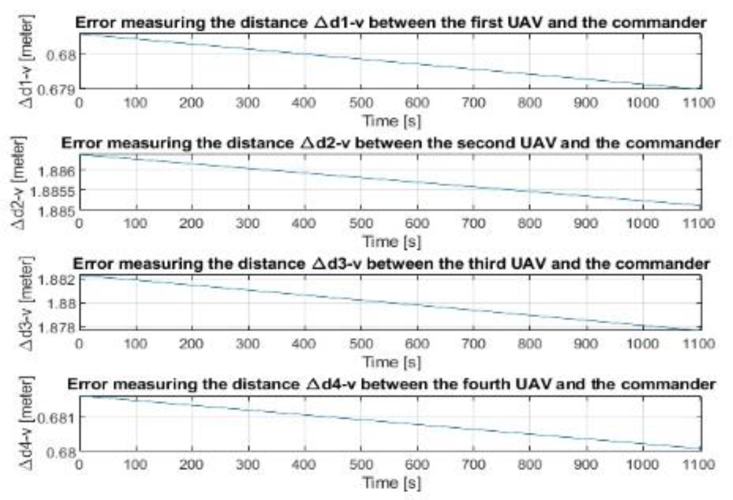
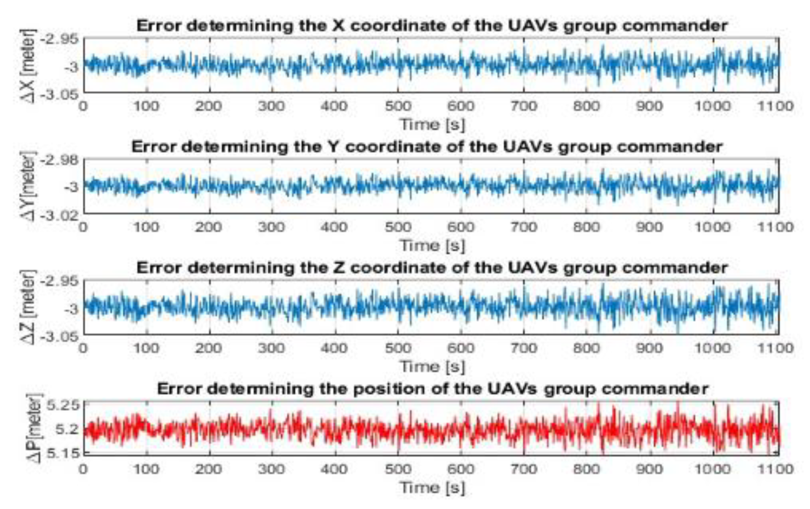
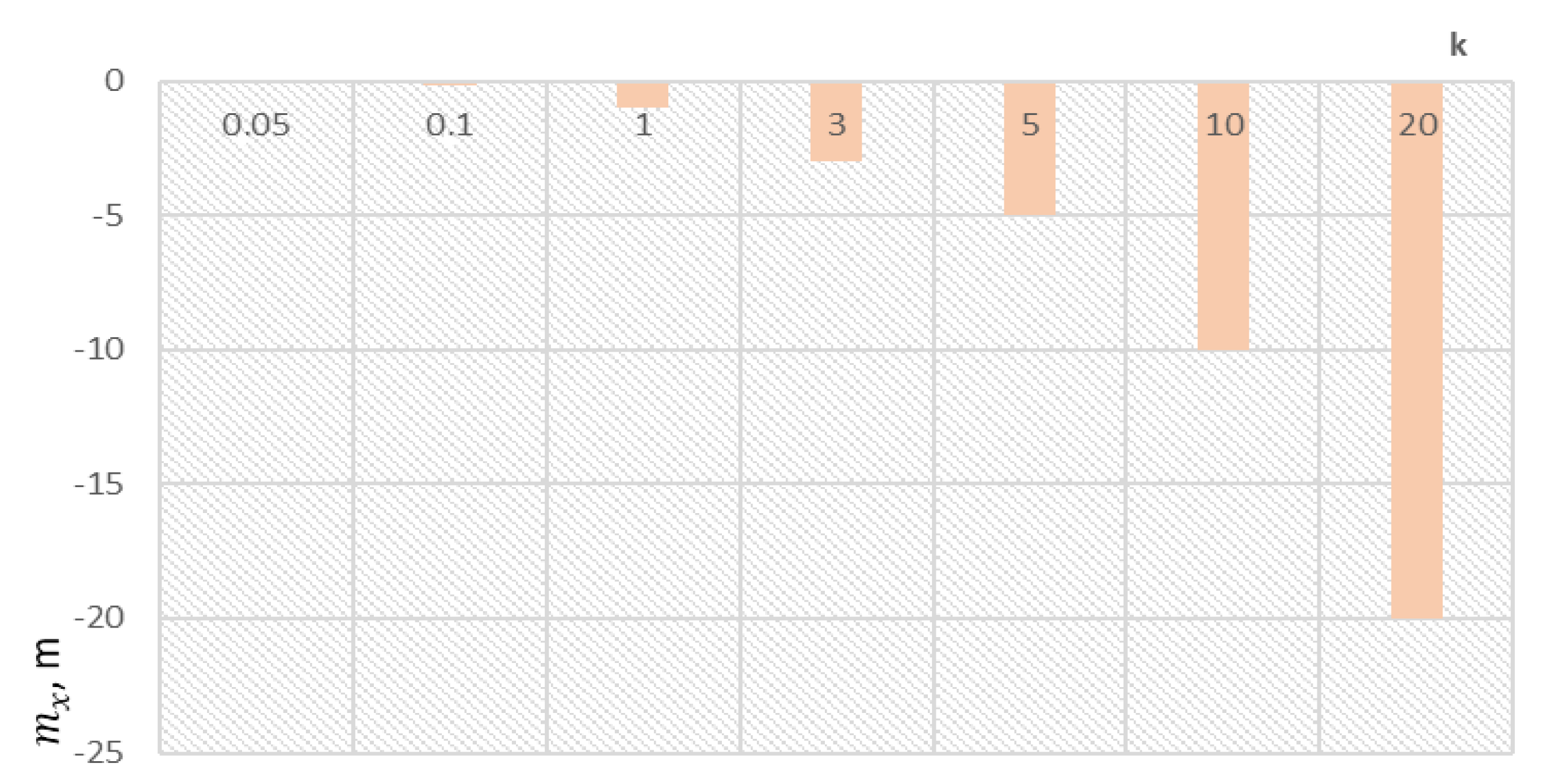
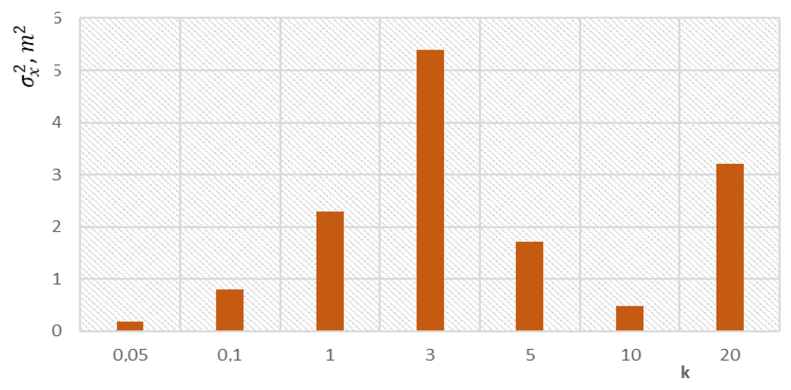
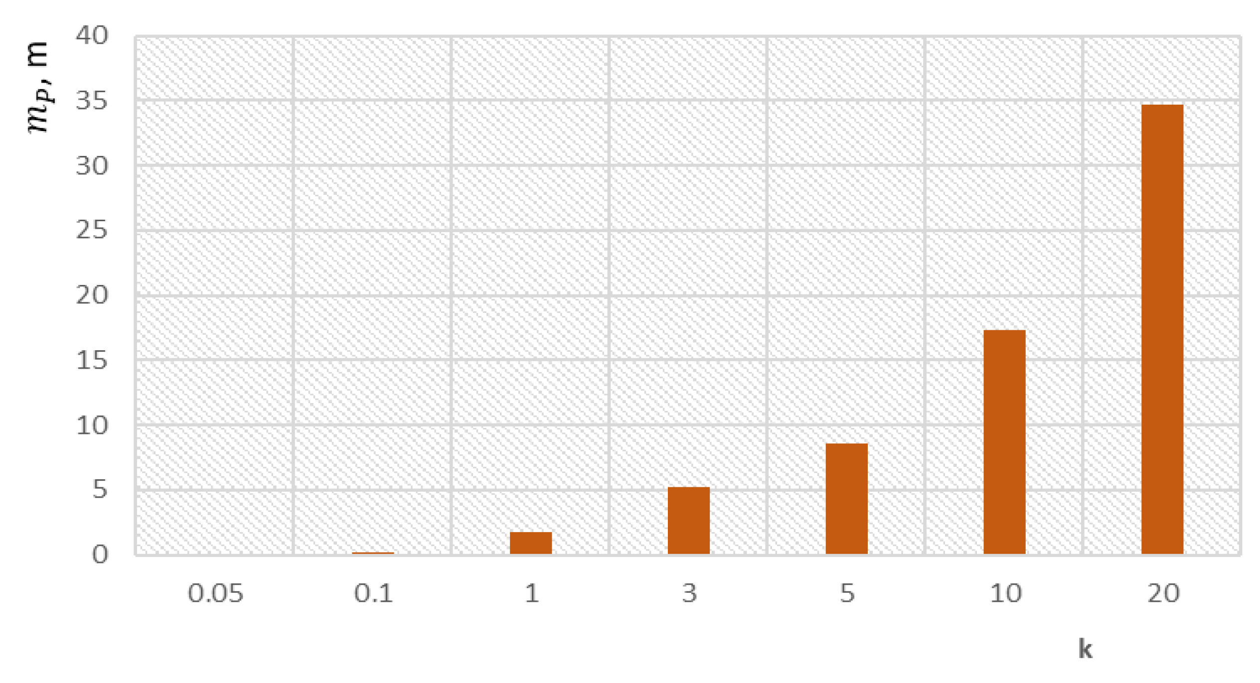
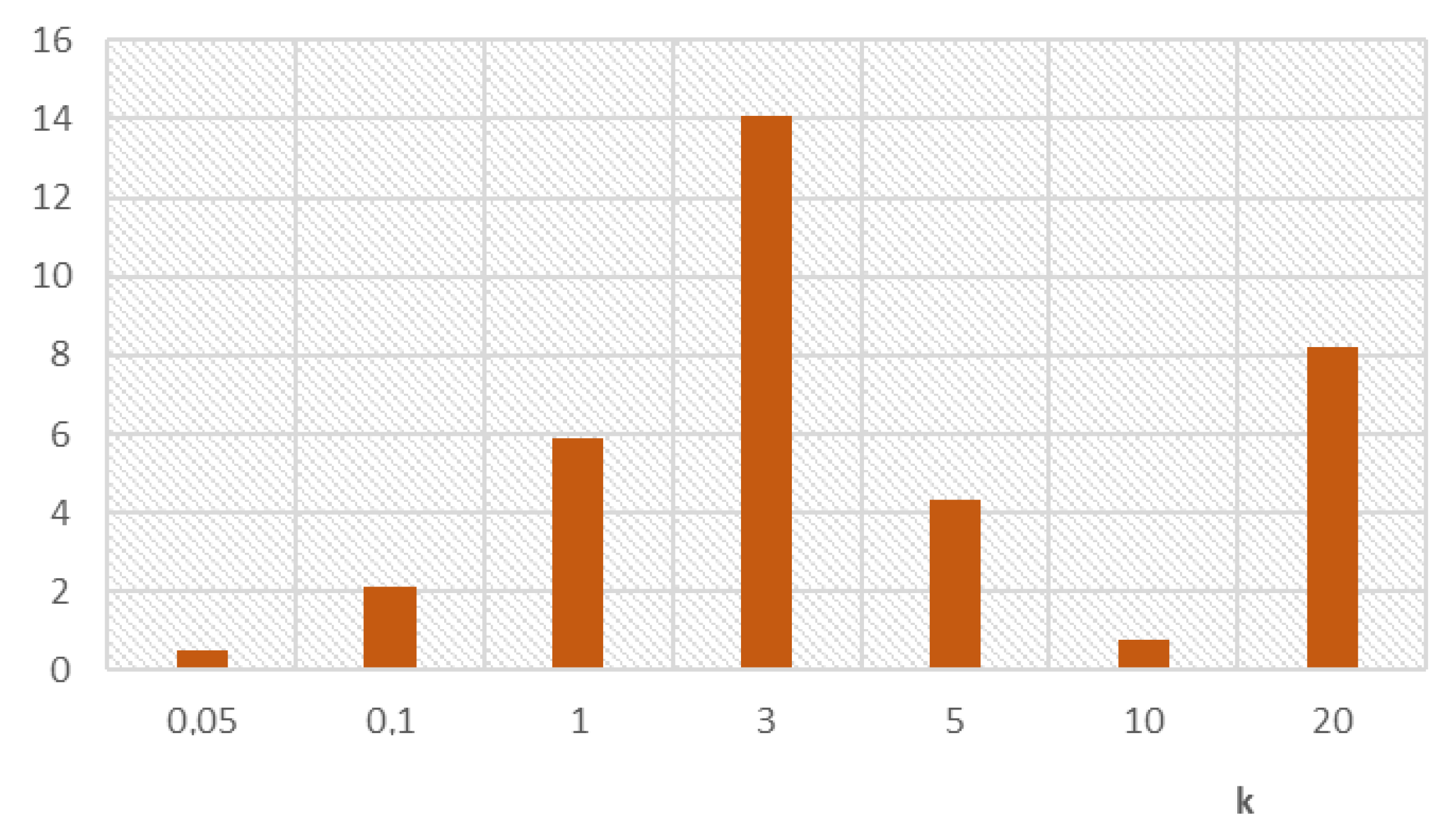
2.4. The Accuracy of Determining the Position of the Selected Member of the Group When Flying in a Group of UAVs
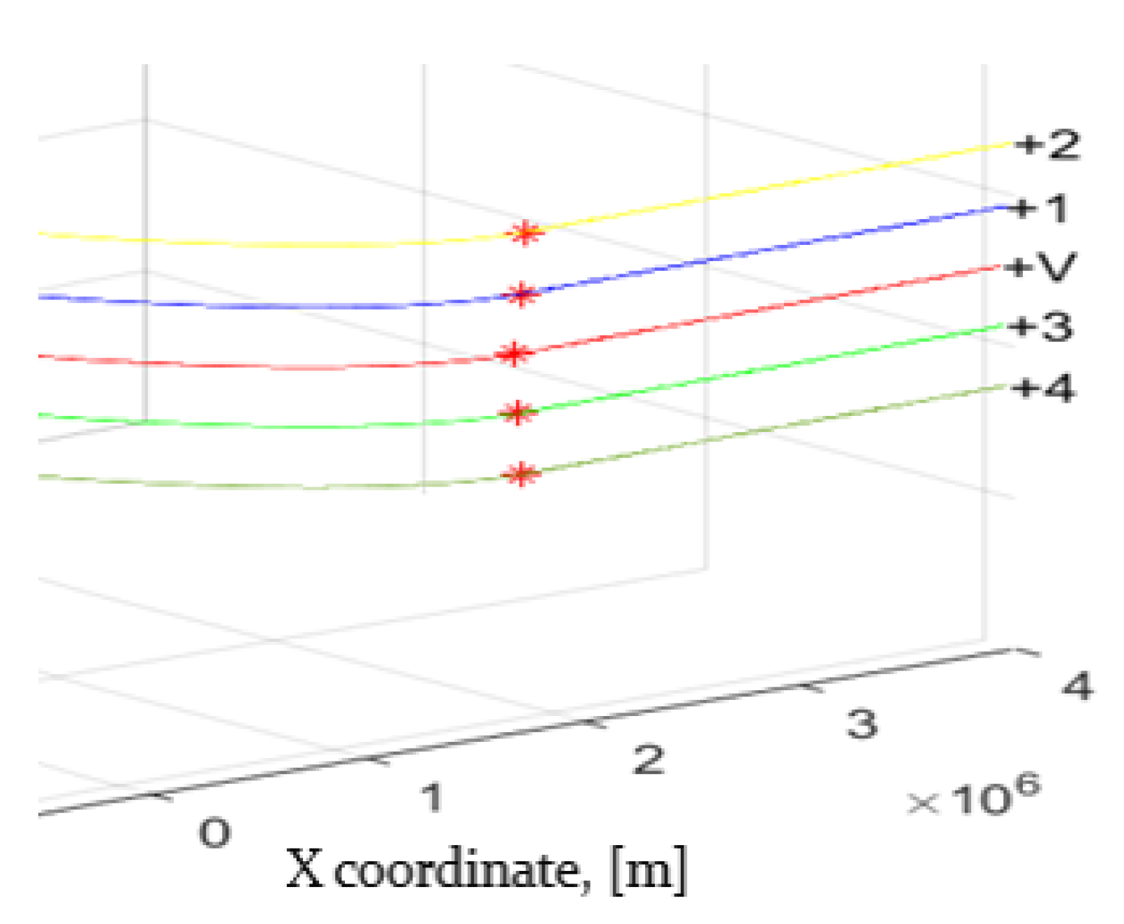
3. Discussion and Results of the Evaluation Accuracy of Determination of the Positioning of the Group Commander
4. Conclusions
Author Contributions
Funding
Data Availability Statement
Conflicts of Interest
References
- Huang, G.; Hu, M.; Yang, X.; Lin, P. Multi-UAV Cooperative Trajectory Planning Based on FDS-ADEA in Complex Environments. Drones 2023, 7, 55. [Google Scholar] [CrossRef]
- Li, B.; Gan, Z.; Chen, D.; Aleksandrovich, S. UAV Maneuvering Target Tracking in Uncertain Environments Based on Deep Reinforcement Learning and Meta-Learning. Remote Sens. 2020, 12, 3789. [Google Scholar] [CrossRef]
- Zhang, J.; Yan, J.; Zhang, P.; Kong, X. Design and Information Architectures for an Unmanned Aerial Vehicle Cooperative Formation Tracking Controller. IEEE Access 2018, 6, 45821–45833. [Google Scholar] [CrossRef]
- Li, B.; Yang, Z.P.; Chen, D.Q.; Liang, S.Y.; Ma, H. Maneuvering target tracking of UAV based on MN-DDPG and transfer learning. Def. Technol. 2021, 17, 10. [Google Scholar] [CrossRef]
- Li, Y.; Tian, B.; Yang, Y.; Li, C. Path planning of robot based on artificial potential field method. In Proceedings of the 2022 IEEE 6th Information Technology and Mechatronics Engineering Conference (ITOEC), Chongqing, China, 4–6 March 2022; pp. 91–94. [Google Scholar]
- Zong, C.; Yao, X.; Fu, X. Path Planning of Mobile Robot based on Improved Ant Colony Algorithm. In Proceedings of the 2022 IEEE 10th Joint International Information Technology and Artificial Intelligence Conference (ITAIC), Chongqing, China, 17–19 June 2022; pp. 1106–1110. [Google Scholar]
- Gao, Y. An Improved Hybrid Group Intelligent Algorithm Based on Artificial Bee Colony and Particle Swarm Optimization. In Proceedings of the 2018 International Conference on Virtual Reality and Intelligent Systems (ICVRIS), Hunan, China, 10–11 August 2018; pp. 160–163. [Google Scholar]
- Sahu, A.; Kandath, H.; Krishna, K.M. Model predictive control based algorithm for multi-target tracking using a swarm of fixed wing UAVs. In Proceedings of the 2021 IEEE 17th International Conference on Automation Science and Engineering (CASE), Lyon, France, 23–27 August 2021; pp. 1255–1260. [Google Scholar]
- Wang, D.; Wu, M.; He, Y.; Pang, L.; Xu, Q.; Zhang, R. An HAP and UAVs Collaboration Framework for Uplink Secure Rate Maximization in NOMA-Enabled IoT Networks. Remote Sens. 2022, 14, 4501. [Google Scholar] [CrossRef]
- Wang, D.; He, T.; Zhou, F.; Cheng, J.; Zhang, R.; Wu, Q. Outage-driven link selection for secure buffer-aided networks. Sci. China Inf. Sci. 2022, 65, 182303. [Google Scholar] [CrossRef]
- Hu, X.; Cheng, J.; Zhou, M.; Hu, B.; Jiang, X.; Guo, Y.; Bai, K.; Wang, F. Emotion-aware cognitive system in multi-channel cognitive radio ad hoc networks. IEEE Commun. Mag. 2018, 56, 180–187. [Google Scholar] [CrossRef]
- Nie, Z.; Zhang, X.; Guan, X. UAV formation flight based on the artificial potential force in 3D environment. In Proceedings of the 2017 29th Chinese Control and Decision Conference (CCDC), Chongqing, China, 28–30 May 2017; pp. 5465–5470. [Google Scholar]
- Cetin, O.; Yilmaz, G. Real-time autonomous UAV formation flight with collision and obstacle avoidance in the unknown environment. J. Intell. Robot. Syst. 2016, 84, 415–433. [Google Scholar] [CrossRef]
- Ming, Z.; Lingling, Z.; Xiaohong, S.; Peijun, M.; Yanhang, Z. Improved Discrete Mapping Differential Evolution for Multi-Unmanned Aerial Vehicles Cooperative Multi-Targets Assignment under Unified Model. Int. J. Mach. Learn. Cybern. 2017, 8, 765–780. [Google Scholar] [CrossRef]
- Chai, X.; Zheng, Z.; Xiao, J.; Yan, L.; Qu, B.; Wen, P.; Wang, H.; Zhou, Y.; Sun, H. Multi-Strategy Fusion Differential Evolution Algorithm for UAV Path Planning in Complex Environment. Aerosp. Sci. Technol. 2022, 121, 107287. [Google Scholar] [CrossRef]
- Sun, X.; Zhang, B.; Chai, R.; Tsourdos, A.; Chai, S. UAV Trajectory Optimization Using Chance-Constrained Second-Order Cone Programming. Aerosp. Sci. Technol. 2022, 121, 107283. [Google Scholar] [CrossRef]
- Beinarovica, A.; Gorobetz, M.; Levchenkov, A. The control algorithm of multiple unmanned electrical aerial vehicles for their collision prevention. In Proceedings of the 12th International Conference on Intelligent Technologies in Logistics and Mechatronics Systems (ITELMS), Panevezys, Lithuania, 26–27 April 2018; pp. 37–43. [Google Scholar]
- Graffstein, J. Functioning of an air anti-collision system during the test flight. Aviation 2014, 18, 44–51. [Google Scholar] [CrossRef]
- Zhao, W.; Li, L.; Wang, Y.; Zhan, H.; Fu, Y.; Song, Y. Research on A Global Path-Planning Algorithm for Unmanned Arial Vehicle Swarm in Three-Dimensional Space Based on Theta*–Artificial Potential Field Method. Drones 2024, 8, 125. [Google Scholar] [CrossRef]
- Zhang, S.; Xu, M.; Wang, X. Research on Obstacle Avoidance Algorithm of Multi-UAV Consistent Formation Based on Improved Dynamic Window Approach. In Proceedings of the 2022 IEEE Asia-Pacific Conference on Image Processing, Electronics and Computers (IPEC), Dalian, China, 14–16 April 2022; pp. 991–996. [Google Scholar]
- Jing, X.; Hou, M.; Wu, G.; Ma, Z.; Tao, Z. Research on maneuvering decision algorithm based on improved deep deterministic policy gradient. IEEE Access 2022, 10, 92426–92445. [Google Scholar]
- Fujimoto, S.; Hoof, H.; Meger, D. Addressing function approximation error in actor-critic methods. In International Conference on Machine Learning; PMLR: New York, NY, USA, 2018; pp. 1587–1596. [Google Scholar]
- Zhang, S.; Li, Y.; Dong, Q. Autonomous navigation of UAV in multiobstacle environments based on a Deep Reinforcement Learning approach. Appl. Soft Comput. 2022, 115, 108194. [Google Scholar] [CrossRef]
- Zhang, H.; Huang, C.; Xuan, Y.; Tang, S. Maneuver decision of autonomous air combat of un-manned combat aerial vehicle based on deep neural network. Acta Armamentaria 2020, 41, 1613–1622. [Google Scholar]
- Luo, Y. Research on Air Combat Decision Method Based on Dynamic Bayesian Network; Shenyang Aerospace University: Shen Yang, China, 2018; pp. 1–62. [Google Scholar]
- Dzunda, M.; Dzurovcin, P.; Melniková, L. Determination of Flying Objects Position. In TransNav: The International Journal on Marine Navigation and Safety of Sea Transportation; Vol. 13 No.2-june 2019; Faculty of Navigation: Gdyňa, Poľsko, 2019; pp. s423–s428. [Google Scholar]
- Džunda, M.; Kotianová, N.; Dzurovčin, P.; Szabo, S.; Jenčová, E.; Vajdová, I.; Košcák, P.; Liptáková, D.; Hanák, P. Selected Aspects of Using the Telemetry Method in Synthesis of RelNav System for Air Traffic Control. Int. J. Environ. Res. Public Health 2020, 17, 213. [Google Scholar] [CrossRef] [PubMed]


| UAV Marking | Coordinates WGS 84 | MSL, m | Flight Height, m | Coordinates JTSK | ||
|---|---|---|---|---|---|---|
| X, km | Y, km | Z, km | ||||
| ZP_V | N48 37 43.5 E19 37 09.2 | 905 | 1850.0 | 3979.461 | 1418.527 | 4764.761 |
| ZP_1 | N48 37 53.4 E19 36 54.6 | 884.0 | 1850.0 | 3979.345 | 1418.168 | 4764.963 |
| ZP_2 | N48 38 03.9 E19 36 40.7 | 814.0 | 1850.0 | 3979.211 | 1417.818 | 4765.177 |
| ZP_3 | N48 37 34.0 E19 36 53.9 | 865.0 | 1850.0 | 3979.774 | 1418.306 | 4764.567 |
| ZP_4 | N48 37 24.4 E19 36 39.1 | 844.0 | 1850.0 | 3980.085 | 1418.095 | 4764.371 |
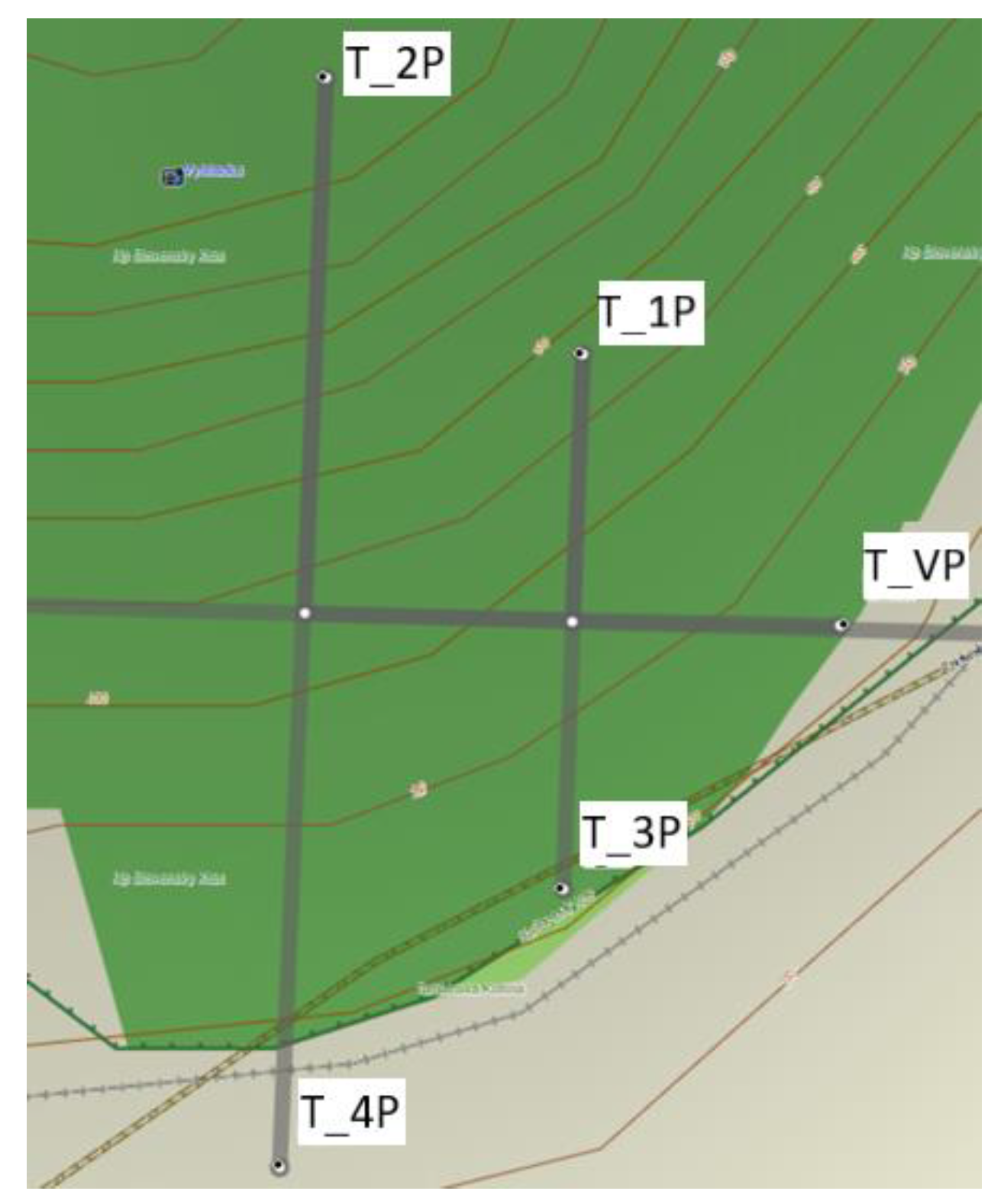
| UAV Marking | Coordinates WGS 84 | MSL, m | Flight Height, m | Coordinates JTSK | ||
|---|---|---|---|---|---|---|
| X, km | Y, km | Z, km | ||||
| T_VP | N48 36 25.4 E20 44 14.5 | 253.0 | 1850.0 | 3952.715 | 1496.553 | 4763.165 |
| T_1P | N48 36 35.3 E20 44 00.1 | 367.0 | 1850.0 | 3952.605 | 1496.196 | 4763.368 |
| T_2P | N48 36 45.3 E20 43 46.0 | 580.0 | 1850.0 | 3952.396 | 1496.093 | 4763.572 |
| T_3P | N48 36 15.9 E20 43 59.0 | 247.0 | 1850.0 | 3953.034 | 1496.334 | 4762.971 |
| T_4P | N48 36 05.9 E20 43 43.4 | 236.0 | 1850.0 | 3953.364 | 1496.117 | 4762.767 |
| Name | Coordinates of the Group Commander of the UAVs | ||
|---|---|---|---|
| X, m | Y, m | Z, m | |
| ZP_V | 3,979,461.0 | 1,418,527.0 | 4,764,761.0 |
| ZP_VS | 3,979,461.0 | 1,418,527.0 | 4,764,761.0 |
Disclaimer/Publisher’s Note: The statements, opinions and data contained in all publications are solely those of the individual author(s) and contributor(s) and not of MDPI and/or the editor(s). MDPI and/or the editor(s) disclaim responsibility for any injury to people or property resulting from any ideas, methods, instructions or products referred to in the content. |
© 2024 by the authors. Licensee MDPI, Basel, Switzerland. This article is an open access article distributed under the terms and conditions of the Creative Commons Attribution (CC BY) license (https://creativecommons.org/licenses/by/4.0/).
Share and Cite
Džunda, M.; Dzurovčin, P.; Čikovský, S.; Melníková, L. Determining the Location of the UAV When Flying in a Group. Aerospace 2024, 11, 312. https://doi.org/10.3390/aerospace11040312
Džunda M, Dzurovčin P, Čikovský S, Melníková L. Determining the Location of the UAV When Flying in a Group. Aerospace. 2024; 11(4):312. https://doi.org/10.3390/aerospace11040312
Chicago/Turabian StyleDžunda, Milan, Peter Dzurovčin, Sebastián Čikovský, and Lucia Melníková. 2024. "Determining the Location of the UAV When Flying in a Group" Aerospace 11, no. 4: 312. https://doi.org/10.3390/aerospace11040312
APA StyleDžunda, M., Dzurovčin, P., Čikovský, S., & Melníková, L. (2024). Determining the Location of the UAV When Flying in a Group. Aerospace, 11(4), 312. https://doi.org/10.3390/aerospace11040312