Exploring the Aerodynamic Effect of Blade Gap Size via a Transient Simulation of a Four-Stage Turbine

Abstract

With the impact of size on low-pressure turbines (LPTs) increasing, the gap between the blades has shrunk, inevitably influencing the unsteady effects inside the turbine. In this study, the aerodynamic effect of the blade gap size is investigated using a compressible unsteady Reynolds-averaged Navier–Stokes (URANS) model on the basis of a four-stage LPT. Simulations are conducted in which the gap between the third-stage stator (S3) and rotor (R3) varies from 0.2 to 0.8 times the axial chord length of the R3 blade. The multi-stage environment reflects the complexity of real low-Reynolds flow fields. Computational fluid dynamics is used to analyze the flow field in detail. The results demonstrate that in the small-gap (AG-0.2) case, the turbulence kinetic energy (TKE) level of the S3 wake close to the R3 leading edge is four-thirds of that in the large-gap (AG-0.8) case. The higher intensity of the wake impacting on the blade results in a higher inverse pressure gradient in the rear part of the R3 suction surface, which increases the profile loss. However, the AG-0.2 case leads to fewer losses caused by the passage vortex in the hub area under the influence of the higher intensity of the wake.

1. Introduction

Low-pressure turbines (LPTs) are one of the key components of aircraft engines, involving multiple stages and accounting for almost one-third of the weight of the entire engine [1]. High-load blades can effectively reduce the number of stages and blades of low-pressure turbines [2]. However, increasing the blade load inevitably increases the adverse pressure gradient at the suction surface, making it easy to separate the boundary layer. Meanwhile, high-load blades enhance end-zone secondary flows, resulting in a sharp increase in losses. When low-pressure turbines are used in a high-altitude cruising state, the working Reynolds number of the low-pressure turbine blades reaches an extremely low level, which seriously affects the aerodynamic performance of the low-pressure turbines and restricts the application of high-load blades [3]. Previous studies have shown that researching the unsteady effects of the incoming wake can help solve the problems caused by low Reynolds numbers and high-load blades.

Meyer [4] was the first to describe the transportation process of incoming wakes in the blade passage, and he simplified the interaction between the upstream wake and the blade surface into a “negative jet” model. Based on the studies of Hodson and Dawes [5], Mahallati [6] created a disturbance diagram of the upstream wake in a blade passage. Smith [7] found that the wake is cut into two parts by the leading edge of the blade when the wake enters the downstream blade row passage, describing the development process in the blade passage as comprising cutting, bending, stretching, and deformation. Stieger and Hodson [8] demonstrated the wake transportation process in the cascade passage by measuring transient changes in the blade passage’s turbulent kinetic energy with a laser Doppler anemometry experiment, obtaining a similar conclusion to Smith’s [7].

The unsteady transportation process of the upstream wake may directly affect the boundary layer characteristics of low-pressure turbine suction surfaces. Schulte and Hodson [9] studied the interaction between the wake sweep and the blade suction surface separation bubble; they concluded that the wake sweep suppresses boundary layer separation, but the separation bubble recurs periodically within the wake passage interval. Liang et al. [10] tested the wake–boundary layer effect and obtained the changes in the proportion of the separation loss and turbulent friction loss with the wake frequency. The results showed that the two losses display inverse changes compared with the wake frequency, indicating that there is an optimal wake frequency that is the least sum of the two losses. Michelassi et al. [11] analyzed the influence of the frequency of incoming wakes through DNS studies. They found that when the wake frequency is too large, the discrete wake effect ceases to exist and the separation bubble reappears. In addition to the development of the blade boundary layer, the incoming wakes also affect the structure of the secondary flow in the end zone of low-pressure turbines. Schneider et al. [12] found that the passage vortex and the wake of the upstream stator show a strong, unsteady interaction after entering the downstream blade passage, significantly weakening the intensity of the passage vortex generated by the rotor blade. Qu et al. [13] studied the influence of the periodic wake flow caused by the upstream moving bar through a combined experiment and numerical simulation. The results showed that the incoming wake obviously inhibits the suction surface separation bubble, and the secondary vortex at the end wall decreases significantly near the wake’s passing position.

With the continuous improvement in the thrust-to-weight ratio requirements of modern engines, LPTs are becoming increasingly compact, while stator–rotor gaps are decreasing; however, the impact of this change on the performance of LPTs deserves further study. Pichler et al. [14] altered the gap size between the stator and the rotor from 21.5% to 43% of the rotor chord length using large eddy simulations. It was found that in cases with small gaps, the turbulence kinetic energy levels of the stator wake close to the rotor leading edge are much higher than those in cases with large gaps, due to the shorter area mixing distance. Biester et al. [15] found that the passage vortex shows an increased extension with a larger axial gap, which is attributed to the thicker side-wall boundary layer for the larger axial gap and a corresponding increase in the low-momentum side-wall fluid.

In this study, based on a four-stage low-pressure turbine, transient simulations were conducted in which the axial gap between the third-stage stator (S3) and rotor (R3) ranged from 20% to 80% of the R3 axial chord length. An advantage of researching in a multi-stage environment is that it can ensure that the inlet and outlet conditions of the low-pressure turbine are close to those of a real low-Reynolds situation. Another advantage is that in addition to the wake of S3, the wake of blade rows further upstream can also be captured in the R3 passage using a multi-stage environment, which reflects the complexity of real flow fields.

This study aimed to explore the evolution of flow in different stator–rotor axial gaps and analyze the effects of the upstream wake on the downstream flow field. The rest of this paper is organized as follows: Section 2 outlines the details of the four-stage low-pressure turbine and the numerical methods used. Section 3 presents the computed results from the different cases and discusses the influences of the axial gap. Finally, the conclusion is given in Section 4.

2. Research Methodology

2.1. Low-Pressure Turbine Configurations

The four-stage low-pressure turbine shown in Figure 1 was the basis of this study. In the cylindrical coordinate system (r, θ, z), r is the spanwise (radius) direction, θ is the rotational (circumferential) direction, and z is the streamwise (axial) direction. All the rotor blades had a tip clearance equal to 1% of their own blade height. Each blade row generated its own fluid computation domain, in which the stators remained stationary, while the rotors rotated around the Z axis at 6210 revolutions per minute. The shroud in the rotor domain was also kept stationary to simulate true tip leakage flow. Figure 1 shows the rotation direction of each independent fluid computation domain and the rotor domain.

The blade number of each row was modeled in order to ensure that the computational domains of both stator blades and rotor blades had the same circumferential extents in the URANS computational process. The number of blades in each blade row after modeling treatment is shown in

Table 1. Blade numbers.

Blade Row	Blade Numbers
S1	40
R1	80
S2	80
R2	80
S3	80
R3	80
S4	80
R4	80

. The modeled S1 fluid domain had one blade, and each of the other fluid domains had two blades.

When the axial gap between the S3 and R3 was changed, S3 and the blade rows further upstream remained in their original places, while R3, S4, and R4 moved upstream or downstream simultaneously. Figure 2 shows the third stage of the LPT with three different stator–rotor gaps. Under the design parameters of the LPT, the middle gap (AG-0.5) was equal to 50% of the R3 axial chord length, the small gap (AG-0.2) was equivalent to 0.2 times the R3 axial chord length, and the large gap (AG-0.8) was equivalent to 80% of the R3 axial chord length.

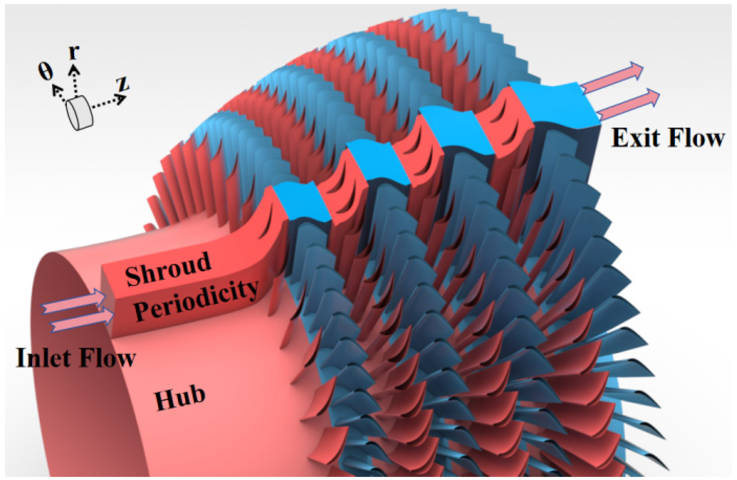
2.2. Numerical Setup and Boundary Conditions

The three-dimensional compressible unsteady Reynolds-averaged Navier–Stokes (URANS) equations were solved using ANSYS CFX v14.0 [16]. The calculation process proceeded on the basis of the results of the convergent steady-state calculation. The transient simulations of the study were conducted using the dual-time-step method proposed by Jameson [17]. The calculation process of the physical time step is displayed in

Table 2. Calculation process of the physical time step.

Parameters	Values
Rotation speed (RPM)	6210
Rotation speed (RPS)	103.5
Stator blade numbers	80
Number of stationary blade passages passed by the rotor blades per second	80 × 103.5 = 8280
Time required for the rotor blades to traverse a stationary blade passage (s)	1/8280 ≈ 1.21 × 10−4
Selected time step (s)	1 × 10−6
Angle of rotor rotation for the blade passages passed by the rotor blades per second (°)	360/80 = 4.5
Angle of rotor rotation within a single time step (°)	1 × 10−6 × 8280 × 4.5 = 0.03726

. As recommended by Arnone and Pacciani [18], the selected value of the physical time step was set to 1 × 10⁻⁶ s, which is lower than one-hundredth of the time required for the rotor blades to traverse a stationary blade passage.

According to Ref. [19], it is customary to specify the total pressure and temperature and the flow direction at the inlet, along with the static pressure at the outlet, when the energy equation is numerically calculated for subsonic flows. The inlet and outlet boundary conditions are listed in

Table 3. Inlet and outlet conditions.

Parameters	Values
Inlet total temperature (K)	1098.3
Inlet total pressure (kPa)	217.9
Turbulence intensity (%)	5
S1 incidence angle (°)	10
Outlet static pressure (kPa)	37.9

, including an inlet total pressure of 217.9 kPa and an inlet total temperature of 1098.3 K. The angle between the inlet flow and the inlet plane was about 7.27°, amounting to an S1 incidence angle of 10°. The turbulence intensity was set to 5%. At the outlet, the static pressure was 37.9 kPa. The expansion ratio of each individual stage was 1.42, 1.53, 1.54, and 1.50. All blade and end-wall surfaces were set as no-slip boundary surfaces, which means the velocity of the fluid at the wall was zero. Considering the effect of actual manufacturing accuracy, the surface roughness of all blades was set to 0.02 mm.

All the side surfaces of the fluid domains were set as fluid–fluid rotational periodicity interfaces, as shown in Figure 1. In accordance with Ref. [16], the interface between the rotor and the stator was set as the transient rotor–stator interface to simulate the rotation of the rotor in a real engine. In the URANS simulation, the sliding mesh method was used to obtain the transient characteristics of the incoming wakes.

2.3. Turbulence Model Validation

The Reynolds averaging method assumes that the flow field variables in a turbulent flow field consist of a time-averaged component and a turbulent fluctuation component. Therefore, turbulence model validation must be used to select a suitable turbulence model for transient simulations.

Considering the similar working conditions of the LPT in this study and the large amount of published experimental data, the validation of the turbulence model was carried out on a low-pressure turbine component of the E3 engine designed by NASA (Washington, DC, USA) [20] in collaboration with GE. GE (Boston, MA, USA) [21] conducted a series of simulated air tests on the five-stage low-pressure turbine components of an E3 turbine with a 0.67 size scale model test vehicle.

Table 4. E3 low-pressure turbine test parameters.

Parameters	Values
Inlet total temperature (K)	416.7
Inlet total pressure (bar)	3.1
Rotation speed (RPM)	3208.7
Inlet mass (kg/s)	24.4
PT1/PT2	4.37
PT1/PS2	4.76

shows the test state parameters of the E3 low-pressure turbine; our numerical calculation adopts adopted the same boundary conditions as the test.

The radial distributions of circumferential efficiency at the outlet in the experimental data, along with the numerical calculations corresponding to the k-ω of Wilcox (Newington, CT, USA) [22], the k-ε of Launder and Spalding [23], the SST of Menter [24], and the modified RNG k-ε of Yakhot [25], are displayed in Figure 3. It can be seen that the SST model has the greatest similarity with our experimental results.

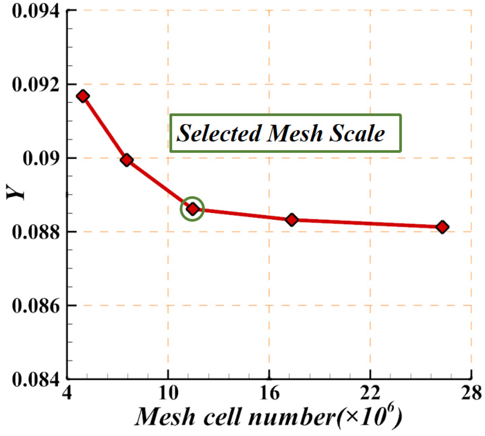
2.4. Mesh Sensitivity Validation

The grid for the transient simulation shown in Figure 4 was generated using NUMECA AutoGrid5 13.1. The grid topology used was O4H, which divides the calculation area into 5 parts. The O-topology grid was used for the area around the blade to guarantee mesh quality, and 4 H-topology grids were used in the main stream regions to obtain better orthogonality. In order to ensure that the thickness of the near-wall mesh met the requirements of the SST model for the y⁺ value, the thickness of the first layer of the mesh was set to 1 × 10⁻⁶ m.

The five different mesh scales used for the sensitivity validation are displayed in

Table 5. Mesh parameters.

Case	1	2	3	4	5
Cell numbers	4,952,960	7,553,792	11,462,528	17,347,840	26,278,656
Average mesh volume (v/m3)	5.24 × 10−11	7.93 × 10−11	1.20 × 10−10	1.82 × 10−10	2.78 × 10−10
Average mesh size (L/m)	0.65 × 10−3	0.57 × 10−3	0.49 × 10−3	0.43 × 10−3	0.37 × 10−3
Mean orthogonal quality	0.897	0.906	0.909	0.911	0.913
Mean determinant	0.959	0.962	0.968	0.972	0.975
Min determinant	0.376	0.325	0.345	0.332	0.359
Mean quality	0.931	0.933	0.934	0.932	0.930

. Several parameters are used to evaluate the mesh quality. Orthogonal quality is used to evaluate the degree to which the angle between adjacent cell faces or edges in a grid is close to a certain optimal angle. Orthogonality has a significant impact on simulation accuracy because of its close relation to the calculation of variable gradients, viscosity, and convective flux. Determinant checking characterizes the deformation of elements by calculating the Jacobian determinant values for each hexahedron and then standardizing the matrix of the determinant. The quality is a weighted diagnostic between Determinant, Max Orthogls, and Max Warpgls. For these parameters, a value of 1 represents an ideal hexahedral cube, while 0 represents an inverse cube with a negative volume.

Figure 5 shows the mesh convergence result of the Y value of R1 at five mesh numbers. When the cell numbers increased from 11.5 million to 17.3 million, the variation in Y was less than 0.35%. Therefore, after considering the calculation speed and accuracy comprehensively, the cell number of the grid for this study was set to 11.5 million.

3. Results and Discussion

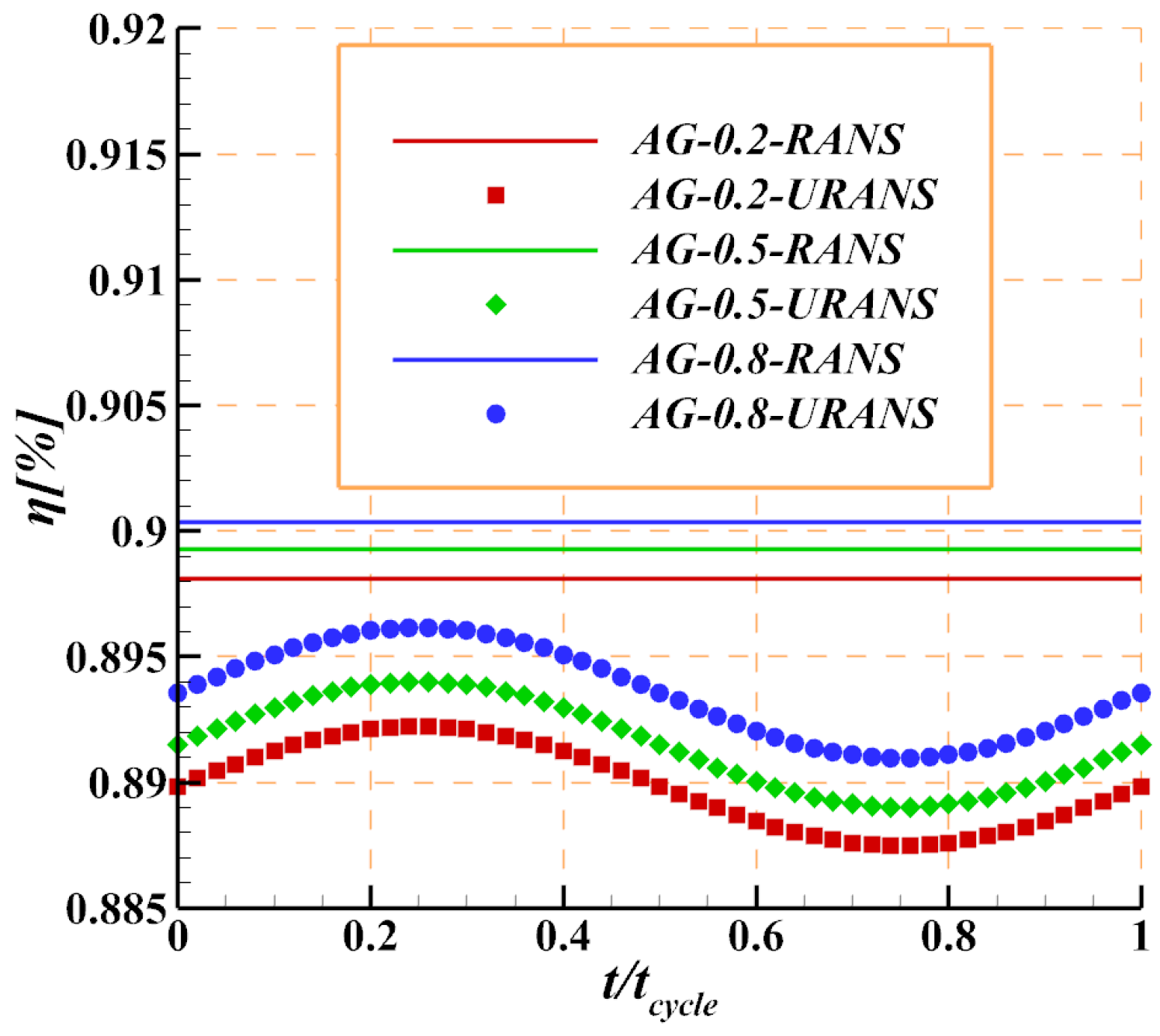
3.1. Aerodynamic Characteristics

In the actual operation process, LPTs face constant changes in the expansion ratio. In order to find out the aerodynamic performance of the turbine under different working environments, the pressure ratio of the whole turbine was increased from 4.25 to 7.25 during the steady-state simulation process. Figure 6 compares the variation in efficiency versus the pressure ratio corresponding to AG-0.2, AG-0.5, and AG-0.8. It can be seen that an increase in the pressure ratio leads to a decrease in efficiency in all three cases. The LPT configuration exhibits the highest efficiency in the case of AG-0.8 and the lowest efficiency in the case of AG-0.2 at all pressure ratios. Next, we conducted aerodynamic performance analysis under unsteady conditions for the design operating point of an expansion ratio of 5.75.

Figure 7 compares the variation in turbine stage efficiency over the periods of the cycle corresponding to AG-0.2, AG-0.5, and AG-0.8 to illustrate the impact of the S3–R3 gap size on aerodynamic efficiency. The results calculated from the URANS simulations display characteristic fluctuations in isentropic efficiency over one cycle, while the RANS simulation results remain constant. The relative motion between the stators and the rotors are attributed to the fluctuations in isentropic efficiency. In both RANS and URANS simulations, the efficiency shows the same trend with changes in the S3–R3 gap size.

The total pressure loss coefficient (Y) is widely used to assess the high-loss areas in an LPT. In this study, Y was defined as $Y=\left(P_0^{\ast }-P_1^{\ast }\right)/\left(P_1^{\ast }-P_1\right)$, where $P_0^{\ast }$ is the total inlet pressure, $P_1^{\ast }$ represents the total outlet pressure, and P₁ is the static outlet pressure. Figure 8 shows the time-averaged radial distribution of circumferential Y at 0.3 times the axial chord length behind R3, corresponding to AG-0.2, AG-0.5, and AG-0.8. In the tip region, the differences in momentum and flow direction between the leakage flow and the main stream lead to the high-loss area of the tip leakage vortex (TLV). At 10~90% blade heights, the profile loss is the main contributor. In most parts of this region, the loss shows a trend of reduction when the gap distance is increased. However, the opposite trend occurs in the hub area. AG-0.8 shows the highest loss under the influence of the passage vortex (PV). Overall, a larger S3–R3 gap indicates lower losses in the main stream area and higher losses in the hub area. For LPT blades with large aspect ratios, the loss of the main stream area dominates, leading to changes in the turbine efficiency, as shown in Figure 7.

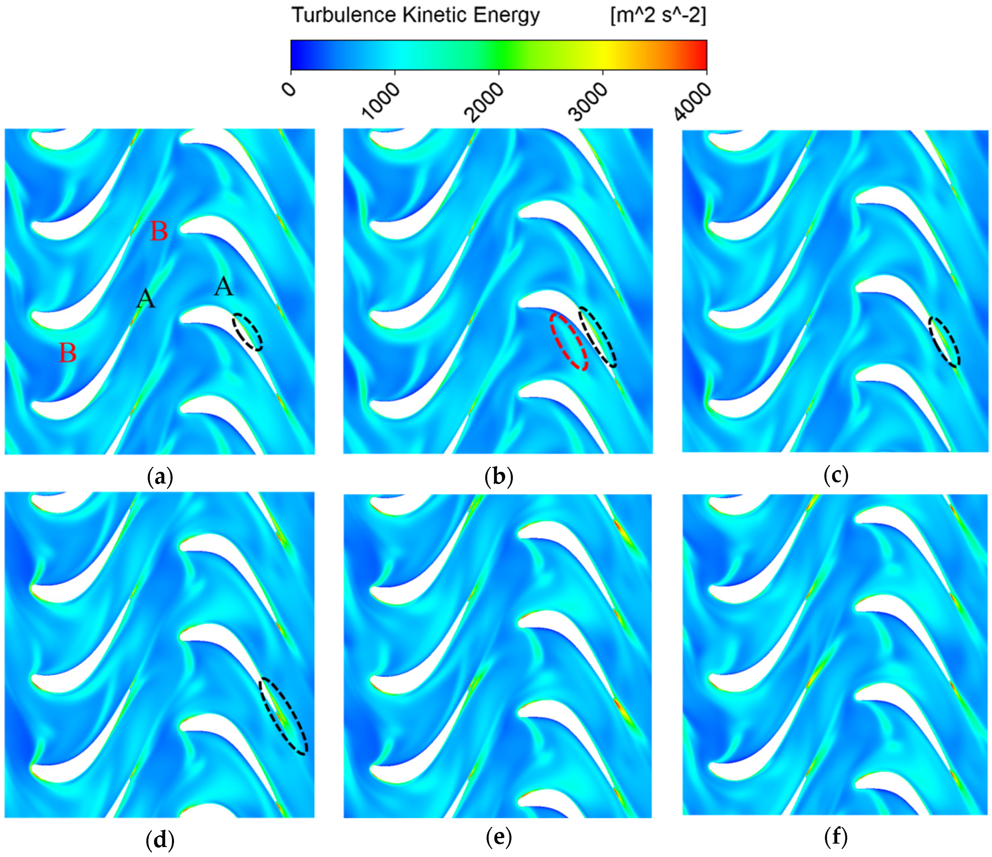
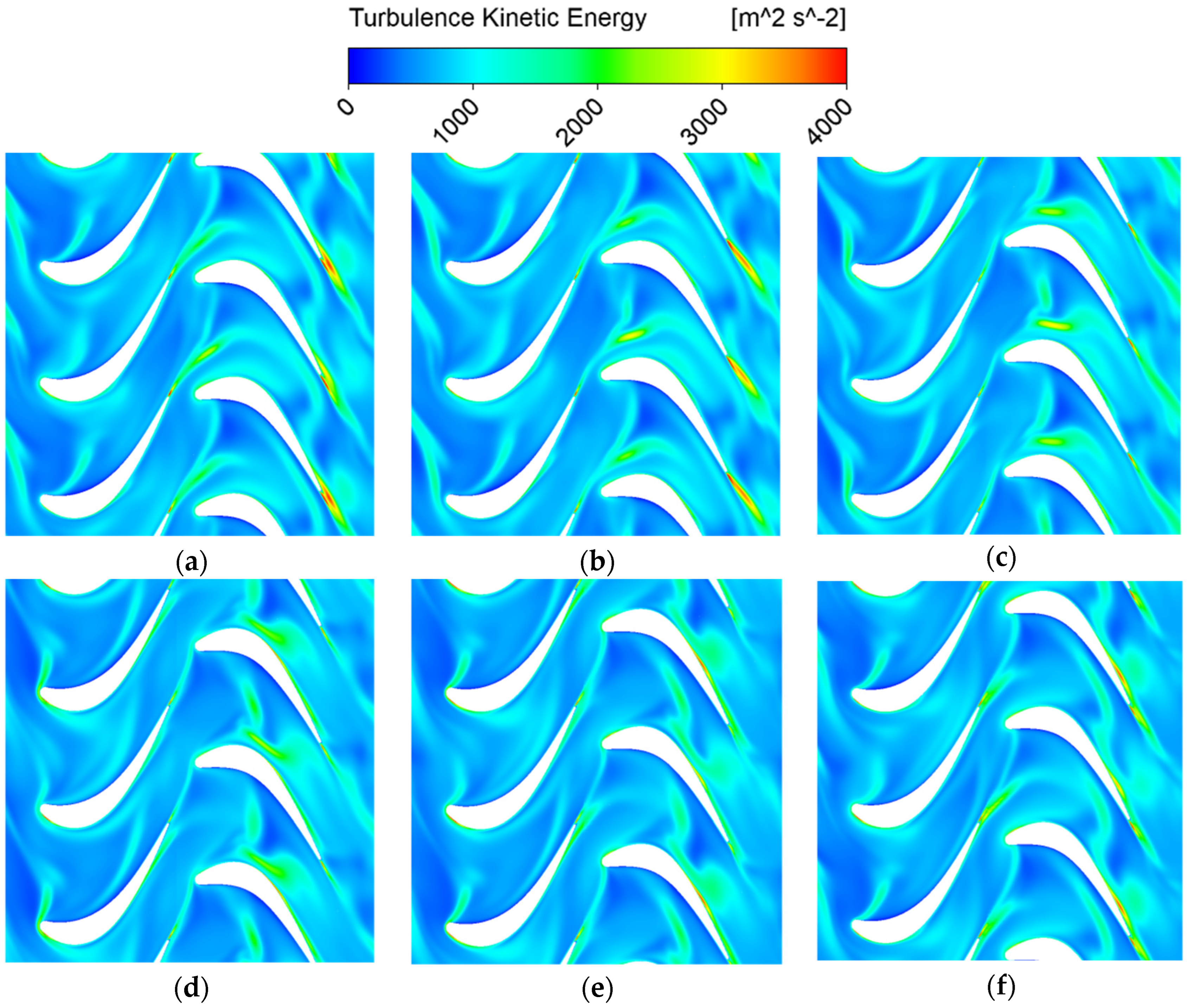
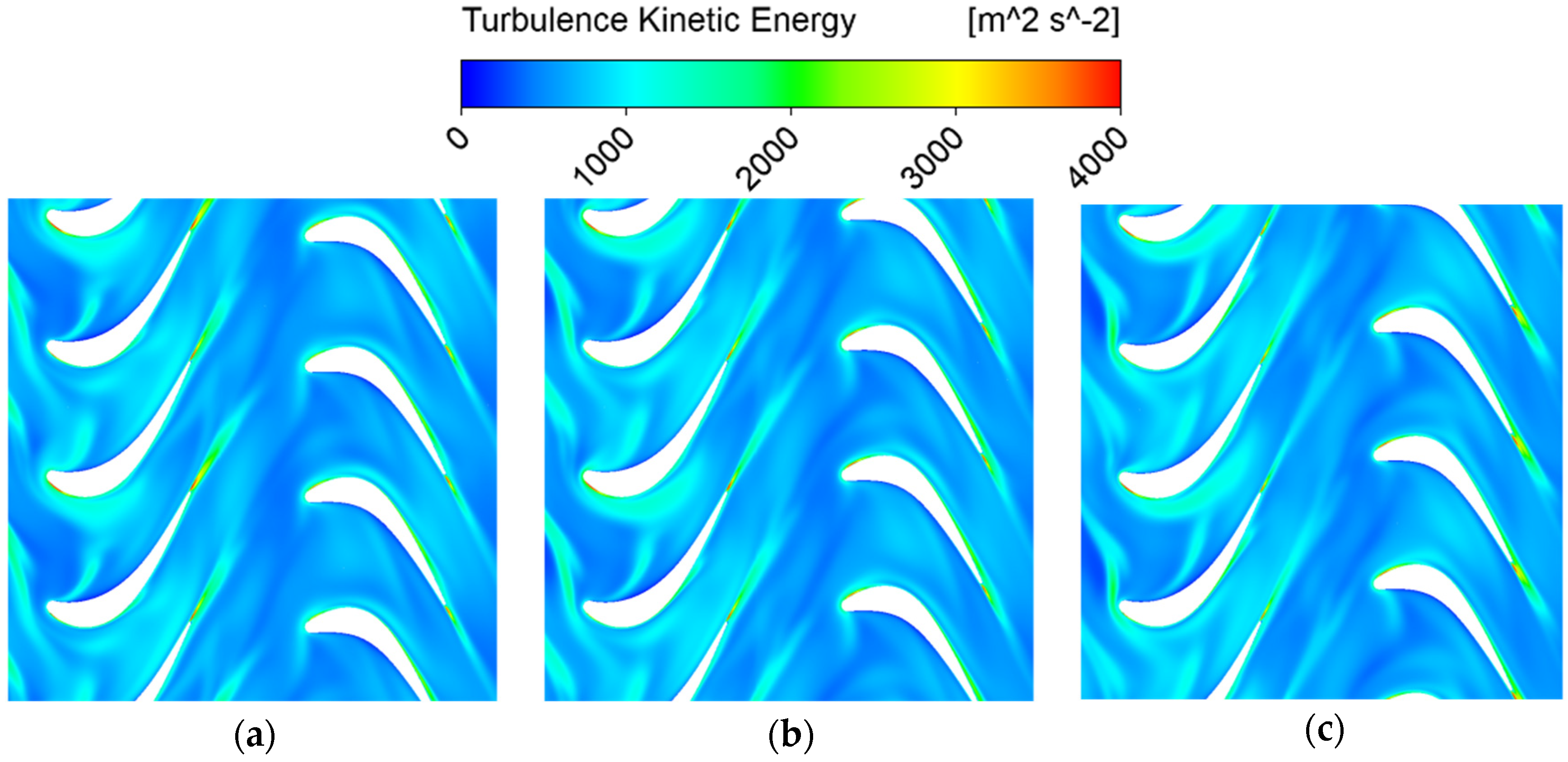
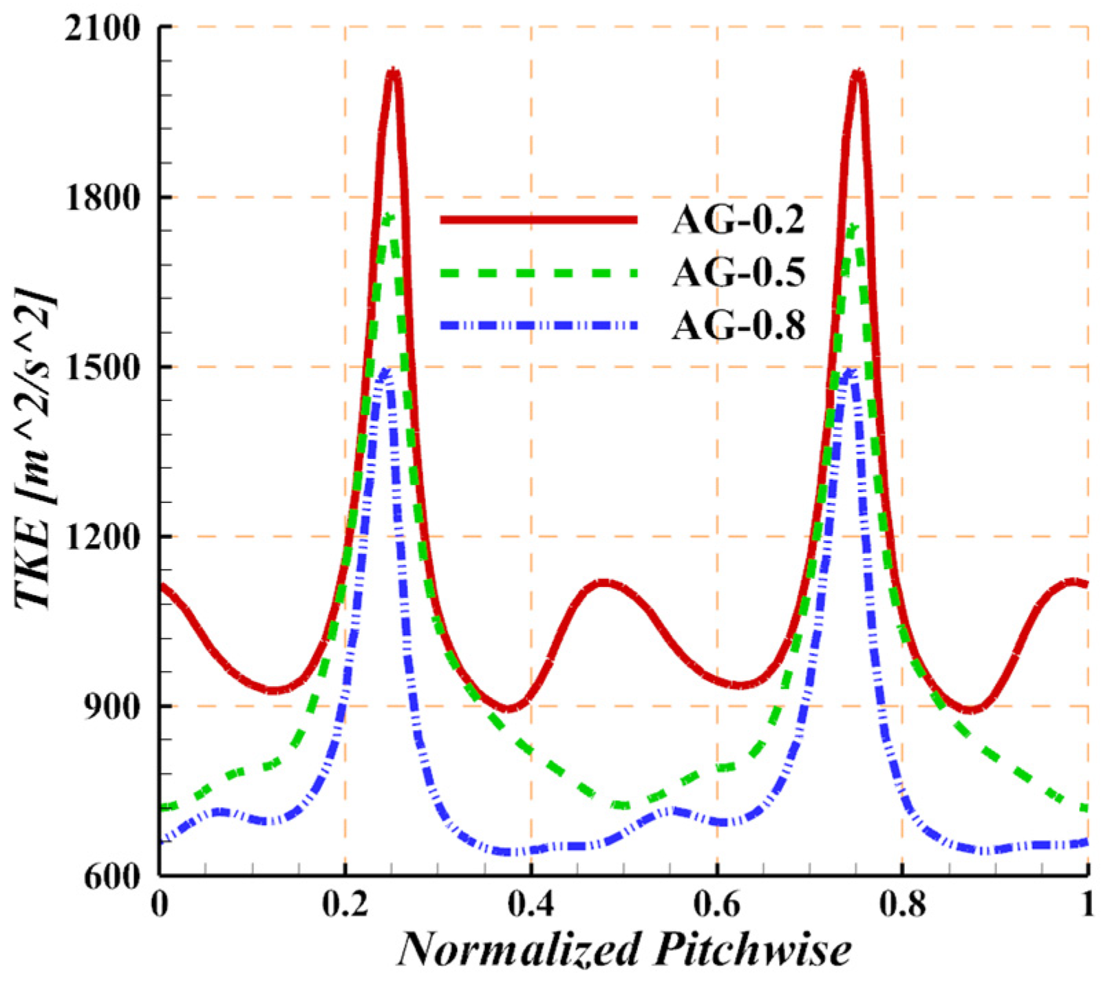
3.2. Transport Structure of the Wake in the Flow Field

In this section, the transport process of the wake from the S3 blade row to the R3 blade row is discussed. Turbulence kinetic energy (TKE) is defined as the variance in the fluctuations in velocity and is widely applied in the study of the incoming wake. Figure 9 shows the TKE contours of the third stage, corresponding to the AG-0.5 simulation, at six selected instants of time, t/t_cycle = 1/6, 2/6, 3/6, 4/6, 5/6, and 6/6, where t_cycle is the time required for the rotor to turn through a stator passage. The S3 blade row is located on the left side, and the high levels of TKE highlight the stator wakes. As can be seen from Figure 9a, at least two wake sources enter the third-stage rotor blade row: one directly from the trailing edge of S3 (label A) and the other from blade rows further upstream (label B).

In the engine’s working state, S3 remains stationary, while R3 moves to the upstream wake. When the leading edge of R3 comes in contact with the upstream wake, the upstream wake enters the flow path along R3 from both sides of the leading edge. As a result, the leading edge of the blade is covered by a high amount of turbulent kinetic energy for a long time.

The interaction between the wake and the pressure side mainly occurs near the leading edge of R3. The wake moves downstream after being cut by the leading edge and toward the suction surface circled in Figure 9b at the same time due to the lateral pressure gradient inside the passage. On the suction side of the leading edge, the cut wake continues to adhere to the blade surface when moving downstream. This part of the wake mixes with the wake from the pressure side to form a converged wake. The downstream motion of the converged wake disturbs the flow on the rear part of the suction surface. At t/t_cycle = 1/6, the region that is circled by black dashed lines shows an elevated TKE value at the 70% position of the axial chord on the suction side. The region is transported downstream along the suction side with the converged wake in the coming instants until it departs from the R3 passage at t/t_cycle = 5/6.

Figure 10 shows the TKE contours of the third stage, corresponding to the AG-0.2 simulation, at six selected instants of time, t/t_cycle = 0/6, 1/6, 2/6, 3/6, 4/6, and 5/6, and Figure 11 presents the same corresponding to the AG-0.8 simulation. Combined with the AG-0.5 case shown in Figure 9, it can be seen that the TKE level of the incoming wake in the R3 passage declines significantly with an increase in the axial gap. Reductions in TKE are related to the mixing of the upstream wake and the main stream accompanying the wake transportation process. Compared to the main stream, the wake of upstream blades demonstrates the characteristics of low speed and high pressure. The physical characteristics of the wake continue to approach the main stream until the complete dissipation of the wake during the transportation process. Furthermore, the elevated TKE region mentioned before becomes increasingly apparent with the shortening of the gap, indicating that further research is needed to illustrate wake–blade interactions under different gap conditions.

Figure 12 shows the time-averaged TKE immediately upstream of the leading edge of R3 on the midspan corresponding to three axial gap cases. It can be seen that with an increase in the axial gap, the intensity of the incoming wakes shows obvious decay. In the AG-0.8 case, the turbulent kinetic energy of the incoming wake is only 75% of that in the AG-0.2 case. It should be pointed out that in the main stream region, the turbulent kinetic energy disturbance will be affected by the wake of the blade rows further upstream, which is particularly obvious in the AG-0.2 case. Considering that a wake with a higher level of TKE would definitely have a stronger unsteady effect on downstream blades, the wake in AG-0.2 is defined as the wake with the highest intensity. Therefore, the axial gap settings create upstream wakes of three different intensities, the effects of which are discussed in the following sections.

3.3. Midspan Flow Field Characteristics

As mentioned before, the intensity of the wake when entering the R3 passage changes depending on the axial gap. The influence of this phenomenon on the R3 midspan flow field is discussed in this section.

Figure 13a shows the evolution of the computed contours of velocity corresponding to the AG-0.2 flow field at six different time instants within one cycle time on a circumferential plane located at a 50% spanwise position. The low-speed flow upstream highlights the wake from the S3 blade. The R3 blade touches the upstream wake at t/t_cycle = 1/6 and cuts it into two parts, resulting in a residual wake on the suction surface. At the same instant, the maximum velocity on the suction surface is located at the 50% position of the axial chord. In the following instants, the wake on the suction surface is transported downstream and mixes with the main stream, resulting in the formation of a low-speed area marked by black circles. Subsequently, both the high- and low-speed flows continue downstream along the suction surface. At t/t_cycle = 5/6, a new high-speed flow appears at the 50% position of the axial chord once the residual wake disappears. Finally, the high-speed flow departs from the R3 passage at t/t_cycle = 6/6, while the residual wake in low-speed area departs from the R3 passage at t/t_cycle = 2/6 of the next cycle. This result shows that the flow condition on the suction surface of R3 is periodically influenced by the upstream flow conditions emanating from the S3 stator exit, forming periodic high-speed main stream areas and low-speed wake areas.

For the same time instants considered in and on the same visualization planes located at the same position shown in Figure 13a, the evolutions of the computed contours of velocity corresponding to AG-0.5 and AG-0.8 are shown in Figure 13b,c. Similarly, the upstream wake is cut into two parts after contact with the R3 blade. The residual wake on the suction surface forms a low-speed area and is transported downstream with the high-speed main stream flow. Comparing these three cases, the amplitude of periodic velocity fluctuation on the suction surface caused by the upstream wake of AG-0.8 is smaller than that of AG-0.5, and both are much smaller than that of AG-0.2. The maximum level of velocity on the suction surface is the lowest when the axial gap is at its largest, while the upstream wake has the highest speed.

To display the wake–blade interaction more clearly, Figure 14a shows the loading of the R3 midspan in terms of the pressure coefficient at six different time instants corresponding to AG-0.2. The pressure coefficient in this study is defined as $C_p=(p(x)-p_1)/(p_0^{\ast }-p_1)$, where p₁ represents the outlet static pressure and $p_0^{\ast }$ is the inlet total pressure. The periodic fluctuation of the pressure coefficient can be illustrated in conjunction with Figure 13a. As is displayed in Figure 13a, at t/t_cycle = 1/6, the R3 blade cuts the upstream wake into two parts. The residual wake forms a low-speed area at the front part of the suction surface while the maximum velocity is located at approximately the 50% position of the axial chord, which is less affected by the wake at the instant. Correspondingly, at t/t_cycle = 1/6, Figure 14a shows that an increase in pressure compared with the time-averaged value takes place at the front part of the suction surface, and the minimum pressure is located at approximately the 50% position of the axial chord. The area where the local static pressure increases under the influence of the wake is labeled as “W”, and the location of the minimum pressure is labeled as “M” in Figure 14. At t/t_cycle = 2/6 and t/t_cycle = 3/6, with the downstream motion of the flow and residual wake, the wake-influenced area moves downstream along the suction surface and covers the 50% position of the axial chord. Therefore, the position of the minimum static pressure on the suction surface moves downstream, and the value of the minimum static pressure increases slightly. From t/t_cycle = 4/6 on, the wake-influenced area continues to move downstream, and its influence on the 50% position of the axial chord gradually weakens. As a result, the minimum pressure appears at the 50% position of the axial chord again and gradually decreases to the value at t/t_cycle = 1/6.

Figure 14b,c show the loading of the R3 midspan in terms of the pressure coefficient corresponding to AG-0.5 and AG-0.8 at six different instants in one cycle. It can be seen that the surface load of the blade has similar periodic variations to the AG-0.2 condition; however, the main difference is that with a smaller axial gap in the AG-0.2 case, the pressure coefficient of the R3 midspan has to fluctuate within a larger range, thus demonstrating that under the influence of a stronger upstream wake, the R3 blade has to bear higher loads at certain instants, which inevitably leads to a higher inverse pressure gradient in the rear part of the passage. Another difference appears at the front part of the suction surface, where the stronger upstream wake gives rise to higher pressure at that region in the AG-0.2 case.

Figure 15 compares the time-averaged pressure coefficients of the R3 midspan corresponding to AG-0.2, AG-0.5, and AG-0.8 to evaluate the impact of the wake intensity on the blade load in the mean sense. The results showed that the unsteady sweep of the wake has a great impact on the front part of the R3 blade. The load on the front part is reduced by the higher-intensity wake, while limited variation appears on the rear part.

The influence of the wake on the front part of the blade may be seen throughout the entire blade. The time-averaged circumferential velocity and the inlet flow angle at the leading edge of the R3 blade are shown in Figure 16. Compared with the other two cases, the absolute value of the circumferential velocity of AG-0.2 is significantly reduced. The reduction in the circumferential velocity is mainly caused by the “negative jet” effect of the incoming wake. This reduction is more pronounced near the end zone. A similar trend is shown in relation to the inlet flow angle. The inlet flow angle of AG-0.2 is bigger than that of the other two cases, which actually means that the R3 blade demonstrates a smaller incidence angle. In the end zone, the reduction in the incidence angle reduces the circumferential pressure gradient in the front passage, which benefits the suppression of the theoretical development of horseshoe vortex pressure surface branches. Nevertheless, the suppression of the passage vortex shown in Figure 8 requires more in-depth study.

3.4. Secondary Flow

Compared with high-pressure turbines, the large aspect ratio of low-pressure turbines indicates a smaller secondary flow loss in the end zone. However, with an increase in the aerodynamic loads and improvements in the aero-engine performance requirements of low-pressure turbines, the influences of secondary flow in the end zone have received increasing attention in recent years.

Figure 17 shows the distribution of circumferential time-averaged Y near the hub at 0.3 times the axial chord position behind R3. The high levels of Y displayed in the three cases exhibit similar structures. The two main high-loss structures appearing near the hub are primarily caused by the passage vortex and the corner vortex, as shown in Figure 17a. Comparing the three distribution contours in Figure 17, the scale of the corner vortex remains basically unchanged, while the high-loss area caused by the passage vortex is significantly amplified with an increase in the axial gap.

Figure 18 shows the computed limiting streamlines on the rotor blade surface and Y at different streamwise viewing planes labeled A–E, corresponding to AG-0.2. The downstream motion of the passage vortex along the suction surface results in the formation of flow separation lines marked as S and reattachment lines marked as R in Figure 18a. The area surrounded by S and R can be used to measure the size of the passage vortex. S and R are the migration paths of the suction legs of the passage vortex and the corner vortex, respectively. The evolution of Y over time shows a distinct pattern of variation for slices D and E. A high Y value can reflect the position of the wake in the passage at different times. At t/t_cycle = 1/6, slices A and B show that the wake of the S3 blade reaches the front passage, which is circled by black dotted lines in Figure 18a, while slice D exhibits a relatively small region of a high Y. The size of the region remains stable at t/t_cycle = 2/6, which then declines when the wake of the S3 blade reaches the position where slice D is located at t/t_cycle = 3/6 and t/t_cycle = 4/6 before returning to the unaffected condition at t/t_cycle = 5/6. As soon as the wake passes by slice D, the area behind this is apparently affected by the wake. This indicates that the unsteady upstream wake disturbs the reattachment lines but does not destroy the original flow structure in the end zone. The high-Y region shown in slice E displays a similar trend to slice D but with a valley at t/t_cycle = 5/6 and restoration at t/t_cycle = 6/6 when the wake departs from the R3 passage. Simultaneously, a new wake enters the R3 passage, and the aforementioned process is carried out periodically.

For comparison, Figure 19 shows the computed limiting streamlines on the rotor blade surface and Y at different streamwise viewing planes labeled A–E, corresponding to AG-0.8. Overall, the flow field features in the end zone of AG-0.8 exhibit many similarities to that of AG-0.2. The flow separation lines and reattachment lines marked in Figure 19 are the migration paths of the suction legs of the passage vortex and corner vortex, respectively. The high-Y regions on slices D and E are periodically suppressed under the impact of the incoming wakes. However, compared with AG-0.2, the Y level of the wake entering the R3 passage is much smaller because of the lower wake intensity. As a result, the periodical fluctuation of Y in slice E is within a much smaller range. Furthermore, the separation line and the high-Y region in slice E move upward in the presence of incoming wakes with lower intensity. As a result, the area surrounded by the separation lines and reattachment lines increases significantly, demonstrating a minimal effect on the suppression of the passage vortex.

4. Conclusions

In this work, the influence of variations in the third-stage stator–rotor gap of a four-stage low-pressure turbine is analyzed. Three cases in which the axial gap varies from 0.2 to 0.8 times the axial chord length of the R3 blade are considered and are denoted as AG-0.2, AG-0.5, and AG-0.8. URANS flow computations are used to investigate the unsteady effects of the S3 wake on the downstream blades and flow field. Our conclusions are as follows:

1.

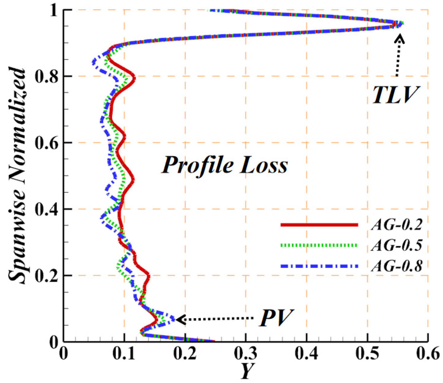
A large blade gap contributes to an increase in efficiency under all variable expansion ratio conditions. The increase in isentropic efficiency when the gap is expanded is attributed to the reduction in the profile losses in the main stream area. When the S3–R3 gap is expanded, the increase in losses in the hub area does not outweigh the reduction in losses in the main stream area, resulting in the highest isentropic efficiency in the case of AG-0.8.

2.

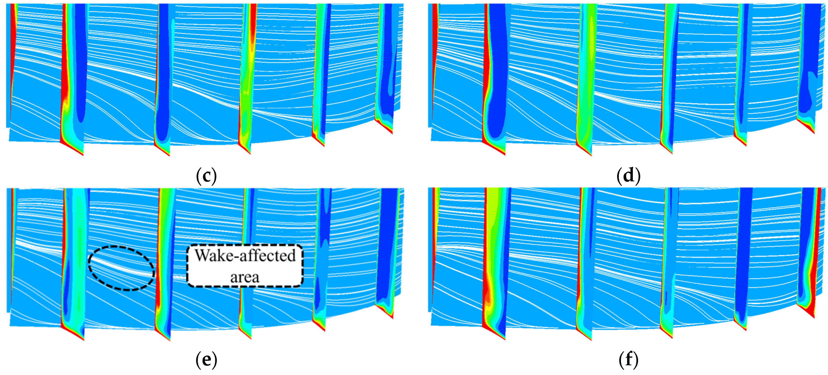
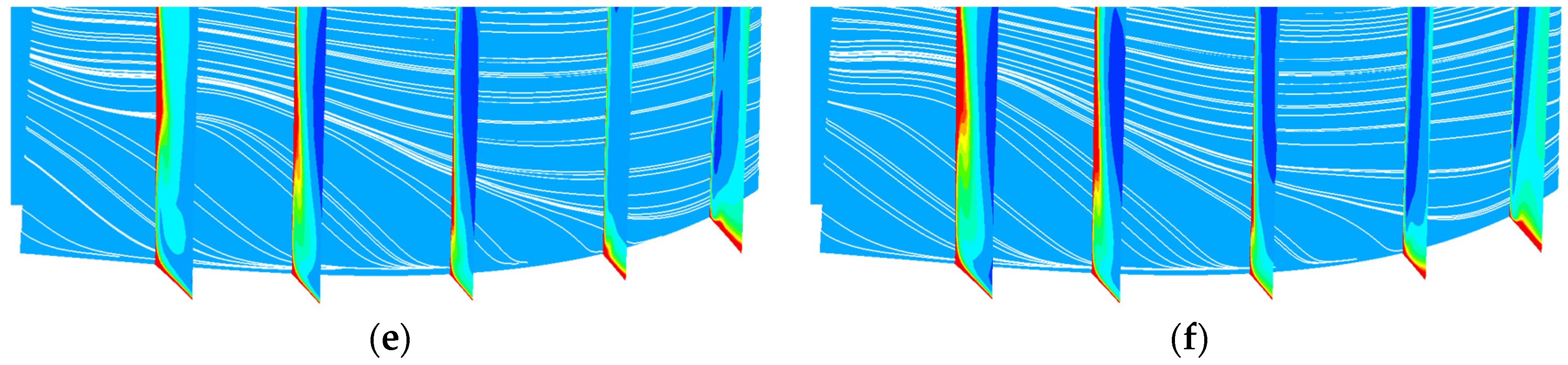
The wake entering the R3 row is reduced significantly when the axial gap is expanded. The reduction in TKE just upstream of the R3 leading edge in AG-0.8 is about 25% compared to that of AG-0.2, which indicates that the intensity of the wake shows obvious decay when mixed with the main stream while being transported downstream.

3.

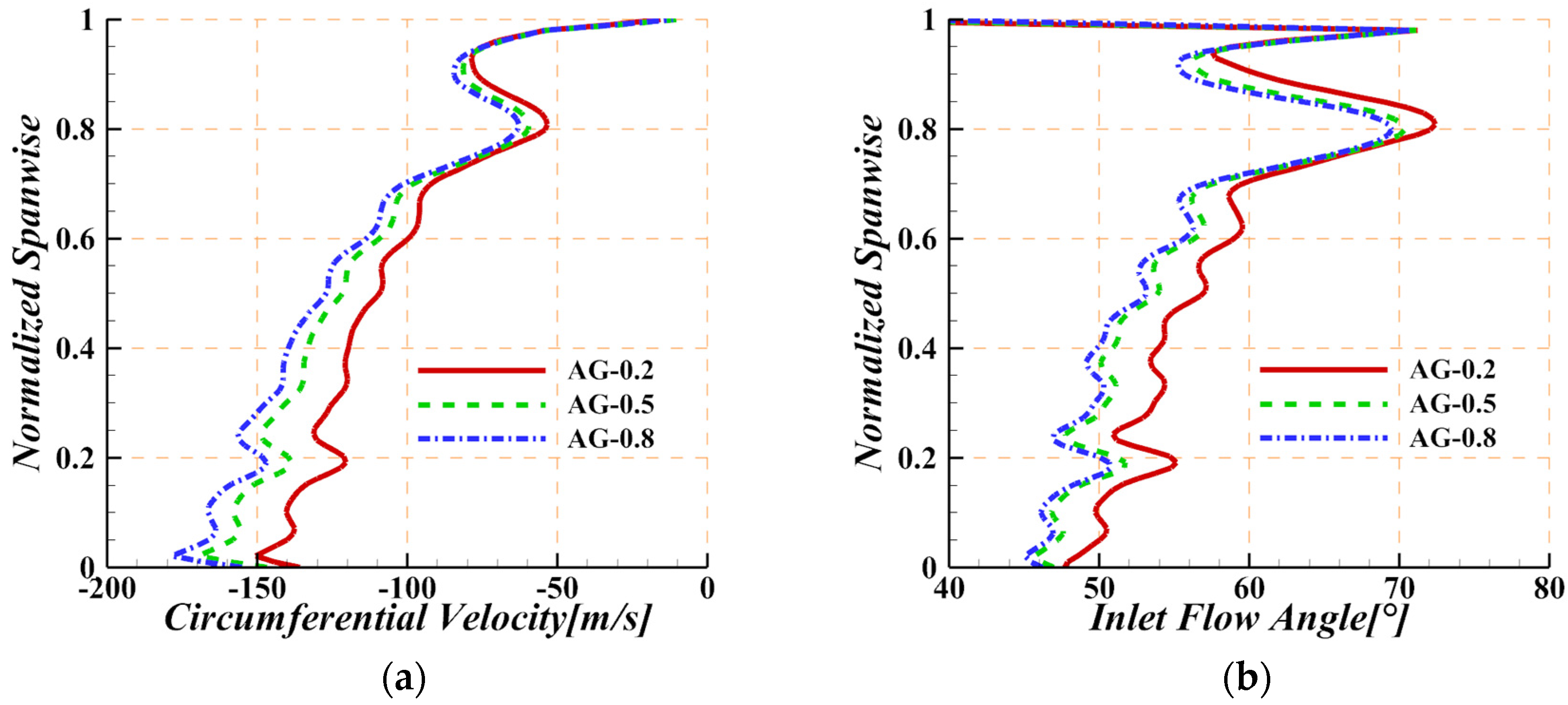
A wake with a stronger intensity leads to a periodic velocity fluctuation of a larger amplitude on the suction surface. Similarly, the unsteady effect of the upstream wake has a larger impact on the load of the R3 blade in the case of AG-0.2, resulting in higher loads at certain instants. Overall, wakes with higher intensity have the greatest impacts on the front part of the R3 blade. The load on the front of the blade is reduced. Meanwhile, the “negative jet” effect caused by a strong wake leads to a reduction in the R3 incidence angle when the S3–R3 gap is reduced.

4.

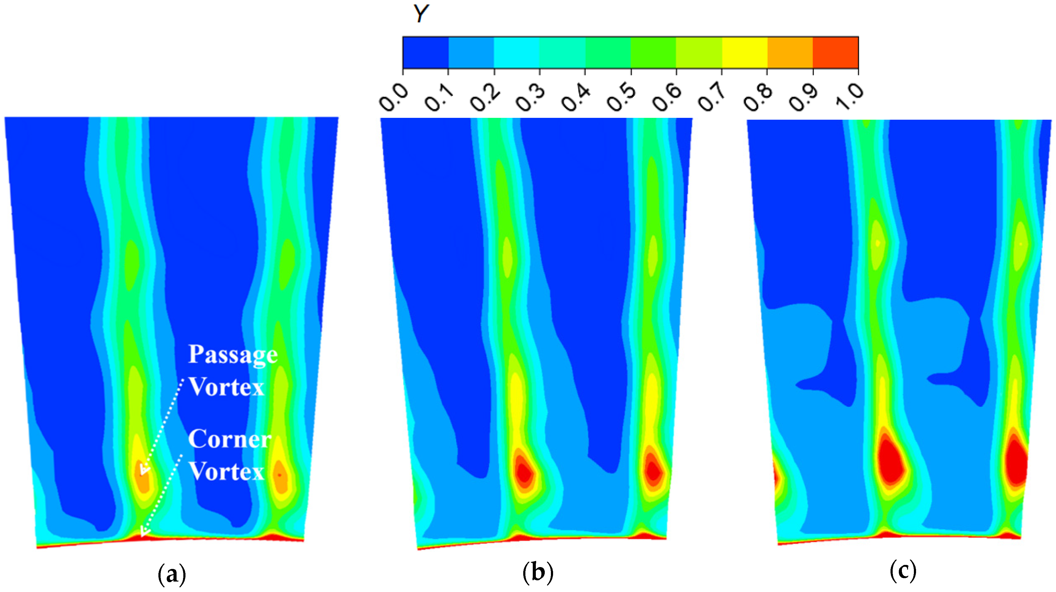
The high-loss regions caused by the passage vortex are periodically reduced by the incoming wakes. In particular, wakes with higher intensity have better effects on passage vortex suppression.

References

1. Curtis, E.; Hodson, H.; Banieghbal, M.; Denton, J.; Howell, R.; Harvey, N. Development of blade profiles for low-pressure turbine applications. J. Turbomach. 1997, 119, 531–538. [Google Scholar] [CrossRef]
2. Howell, R.J.; Hodson, H.P.; Schulte, V.; Stieger, R.D.; Schiffer, H.P.; Haselbach, F.; Harvey, N.W. Boundary layer development in the BR710 and BR715 LP turbines: The implementation of high lift and ultra high lift concepts. J. Turbomach. 1997, 124, 385–392. [Google Scholar] [CrossRef]
3. Mayle, R.E. The 1991 IGTI scholar lecture: The role of laminar-turbulent transition in gas turbine engines. J. Turbomach. 1991, 113, 509–536. [Google Scholar] [CrossRef]
4. Meyer, R.X. The Effects of Wakes on the Transient Pressure and Velocity Distributions in Turbomachines. Trans. Am. Soc. Mech. Eng. 1958, 80, 1544–1551. [Google Scholar] [CrossRef]
5. Hodson, H.P.; Dawes, W.N. On the Interpretation of Measured Profile Losses in Unsteady Wake-Turbine Blade Interaction Studies. J. Turbomach. 1998, 120, 276–284. [Google Scholar] [CrossRef]
6. Mahallati, A. Aerodynamics of a Low-Pressure Turbine Airfoil Under Steady and Periodically Unsteady Conditions. In Proceedings of the ASME Turbo Expo, Vienna, Austria, 6–17 June 2004. [Google Scholar]
7. Smith, L.H. Wake Dispersion in Turbomachines. J. Fluids Eng. 1966, 88, 688–690. [Google Scholar] [CrossRef]
8. Stieger, R.D.; Hodson, P. The Unsteady Development of a Turbulent Wake Through a Downstream Low-Pressure Turbine Blade Passage. J. Turbomach. 2005, 127, 388–394. [Google Scholar] [CrossRef]
9. Schulte, V.; Hodson, H.P. Unsteady wake-induced boundary layer transition in high lift LP turbines. J. Turbomach. 1988, 120, 28–35. [Google Scholar] [CrossRef]
10. Liang, Y.; Zou, Z.P.; Liu, H.X.; Zhang, W.H. Experimental investigation on the effects of wake passing frequency on boundary layer transition in high-lift low-pressure turbines. Exp. Fluids 2015, 56, 81. [Google Scholar] [CrossRef]
11. Michelassi, V.; Chen, L.W.; Pichler, R.; Sandberg, R.D. Compressible direct numerical simulation of low-pressure turbines-part II: Effect of inflow disturbances. J. Turbomach. 2015, 137, 071005. [Google Scholar] [CrossRef]
12. Schneider, C.M.; Schrack, D.; Kuerner, M.; Rose, M.G.; Staudacher, S.; Guendogdu, Y.; Freygang, U. On the Unsteady Formation of Secondary Flow Inside a Rotating Turbine Blade Passage. J. Turbomach. 2014, 136, 061004. [Google Scholar] [CrossRef]
13. Qu, X.; Zhang, Y.; LU, X.; Zhu, J. Unsteady experimental and numerical investigation ofaerodynamic performance in ultra-high-lift LPT. Chin. J. Aeronaut. 2020, 33, 1421–1432. [Google Scholar] [CrossRef]
14. Pichler, R.; Michelassi, V.; Sandberg, R.; Ong, J. Highly Resolved Large Eddy Simulation Study of Gap Size Effect on Low-Pressure Turbine Stage. J. Turbomach. 2018, 140, 21003. [Google Scholar] [CrossRef]
15. Biester, M.H.; Wiegmann, F.; Guendogdu, Y.; Seume, J.R. Time-Resolved Numerical Study of Axial Gap Effects on Labyrinth-Seal Leakage and Secondary Flow in a LP Turbine. In Proceedings of the Turbo Expo: Power for Land, Sea, and Air, San Antonio, TX, USA, 3–7 June 2013; ASME: New York, NY, USA, 2013; Volume 55225. [Google Scholar] [CrossRef]
16. ANSYS Inc. ANSYS CFX 14.0 Solver Theory Guide; ANSYS Inc.: Canonsburg, CA, USA, 2011. [Google Scholar]
17. Jameson, A. Time dependent calculations using multigrid, with applications to unsteady flows past airfoils and wings. In Proceedings of the 10th Computational Fluid Dynamics Conference, Honolulu, HI, USA, 24–26 June 1991. [Google Scholar] [CrossRef]
18. Arnone, A.; Pacciani, R. Rotor-Stator Interaction Analysis Using the Navier–Stokes Equations and a Multigrid Method. J. Turbomach. 1996, 118, 679–689. [Google Scholar] [CrossRef]
19. Yu, J.; Wang, Y.; Song, Y.; Chen, F. Effect of the Honeycomb Tip with Injection on the Aerodynamic Performance in a 1.5-Stage Turbine. J. Turbomach. 2021, 143, 031002. [Google Scholar] [CrossRef]
20. Cherry, D.G.; Gay, C.H.; Lenahan, D.T. Energy Efficient Engine Low Pressure Turbine Test Hardware Detailed Design Report; No. NAS 1.26:167956; NASA Technical Reports Server: Cleveland, OH, USA, 1982. [Google Scholar]
21. Cherry, D.; Dengler, R. The aerodynamic design and performance of the NASA/GE e3 low pressure turbine. In Proceedings of the 20th Joint Propulsion Conference, Cincinnati, OH, USA, 11–13 June 1984. [Google Scholar]
22. Wilcox, D.C. Multiscale model for turbulent flows. AIAA J. 1998, 26, 1311–1320. [Google Scholar] [CrossRef]
23. Launder, B.E.; Spalding, D.B. Lectures in Mathematical Models of Turbulence; Academic Press: London, UK, 1972. [Google Scholar]
24. Menter, F.R. Two-equation eddy-viscosity turbulence models for engineering applications. AIAA J. 1994, 32, 1598–1605. [Google Scholar] [CrossRef]
25. Yakhot, V.; Thangam, S.; Gatski, T.B.; Orszag, S.A.; Speziale, C.G. Development of turbulence models for shear flows by a double expansion technique. Phys. Fluids A Fluid Dyn. 1992, 4, 1510–1520. [Google Scholar] [CrossRef]
Figure 1. Low-pressure turbine configuration.
Aerospace 11 00449 g001
Figure 2. The different blade gap conditions of the third stage: (a) AG-0.2, (b) AG-0.5, and (c) AG-0.8.
Aerospace 11 00449 g002
Figure 3. Turbulence model validation.
Aerospace 11 00449 g003
Figure 4. Mesh configuration.
Aerospace 11 00449 g004
Figure 5. Mesh sensitivity validation.
Aerospace 11 00449 g005
Figure 6. Variation in efficiency with pressure ratio.
Aerospace 11 00449 g006
Figure 7. Variation in efficiency in one cycle.
Aerospace 11 00449 g007
Figure 8. Time-averaged radial distribution of circumferential Y at 0.3 times the axial chord length behind R3, corresponding to AG-0.2, AG-0.5, and AG-0.8.
Aerospace 11 00449 g008
Figure 9. TKE contours at different instants, (a) t/tcycle = 1/6, (b) t/tcycle = 2/6, (c) t/tcycle = 3/6, (d) t/tcycle = 4/6, (e) t/tcycle = 5/6, and (f) t/tcycle = 6/6, corresponding to the AG-0.5 simulation.
Aerospace 11 00449 g009
Figure 10. TKE contours at different instants, (a) t/tcycle = 1/6, (b) t/tcycle = 2/6, (c) t/tcycle = 3/6, (d) t/tcycle = 4/6 (e), t/tcycle = 5/6, and (f) t/tcycle = 6/6, corresponding to the AG-0.2 simulation.
Aerospace 11 00449 g010
Figure 11. TKE contours at different instants, (a) t/tcycle = 1/6, (b) t/tcycle = 2/6, (c) t/tcycle = 3/6, (d) t/tcycle = 4/6, (e) t/tcycle = 5/6, and (f) t/tcycle = 6/6, corresponding to the AG-0.8 simulation.
Aerospace 11 00449 g011aAerospace 11 00449 g011b
Figure 12. Incoming wake intensity just upstream of the R3 leading edge.
Aerospace 11 00449 g012
Figure 13. Velocities at different time instants corresponding to (a) AG-0.2, (b) AG-0.5, and (c) AG-0.8.
Aerospace 11 00449 g013
Figure 14. Distribution of the pressure coefficient variation on the R3 midspan over one cycle corresponding to (a) AG-0.2, (b) AG-0.5, and (c) AG-0.8.
Aerospace 11 00449 g014
Figure 15. Distribution of the time-averaged pressure coefficient on the R3 midspan.
Aerospace 11 00449 g015
Figure 16. Time-averaged (a) circumferential velocity and (b) inlet flow angle at the leading edge of the R3 blade.
Aerospace 11 00449 g016
Figure 17. Time-averaged distribution of Y near the hub at 0.3 times the axial chord length behind R3 corresponding to (a) AG-0.2, (b) AG-0.5, and (c) AG-0.8.
Aerospace 11 00449 g017
Figure 18. Rotor-blade-limiting streamlines and Y at different instants, (a) t/tcycle = 1/6, (b) t/tcycle = 2/6, (c) t/tcycle = 3/6, (d) t/tcycle = 4/6, (e) t/tcycle = 5/6, and (f) t/tcycle = 6/6, corresponding to AG-0.2.
Aerospace 11 00449 g018aAerospace 11 00449 g018b
Figure 19. Rotor-blade-limiting streamlines and Y at different instants, (a) t/tcycle = 1/6, (b) t/tcycle = 2/6, (c) t/tcycle = 3/6, (d) t/tcycle = 4/6, (e) t/tcycle = 5/6, and (f) t/tcycle = 6/6, corresponding to AG-0.8.
Aerospace 11 00449 g019aAerospace 11 00449 g019b