Abstract
Digital elevation models (DEMs), which can provide an accurate description of planetary surface elevation changes, play an important role in scientific tasks such as long-distance path planning, terrain analysis, and planetary surface reconstruction. However, generating high-precision planetary DEMs currently relies on expensive equipment together with complex remote sensing technology, thus increasing the cost and cycle of the task. Therefore, it is crucial to develop a cost-effective technology that can produce high-quality DEMs on the surfaces of planets. In this work, we propose a global attention-based DEM generation network (GADEM) to convert satellite imagery into DEMs. The network uses the global attention mechanism (GAM) together with a multi-order gradient loss function during training to recover precise terrain. The experimental analysis on lunar and Martian datasets not only demonstrated the effectiveness and accuracy of GADEM in bright regions, but also showed its promising reconstruction ability in shadowed regions.
1. Introduction
As global scientific and technological development continues to improve, the Moon, Mars, and other extraterrestrial bodies will become the main targets of human exploration with cutting-edge technology. In these exploration missions, high-quality digital elevation models (DEMs) are crucial. They can provide accurate terrain data and provide key support for landing site selection [1], long-distance path planning [2], and planetary surface reconstruction [3]. Although China’s Chang’e and Wentian series probes and NASA’s Lunar Reconnaissance Orbiter and Mars Reconnaissance Orbiter have acquired high-precision DEMs of the lunar and Martian surfaces, much time has been invested and technology developed. Exploring extraterrestrial bodies like Mars, under the formidable conditions of outer space and the vast interplanetary distances, poses significant challenges. Therefore, there is an urgent need to explore simpler and faster methods to obtain DEMs of planetary surfaces at low cost for use in corresponding downstream tasks.
In recent years, with the advancement of deep learning, numerous studies on DEM generation algorithms have revolved around Convolutional Neural Networks (CNNs) and generative adversarial networks (GANs). Beckham et al. [4] were the first to apply the GAN methodology for the generation of Earth’s DEMs. Panagiotou and colleagues [5] proposed an end-to-end deep learning approach to construct a mapping from RGB images to DEMs. This method allows for the generation of either absolute or relative point cloud estimations of DEMs based on a single RGB satellite or a drone image, thus significantly reducing the cost of acquiring DEMs. However, this method relies on high-resolution image data, which are much scarcer in the planetary scenario, thus limiting its usage. Yao et al. [6] proposed a new continuous representation model (CDEM) using neural networks to obtain elevation values at any location from low-resolution DEM data. Chen et al. [7] introduced Mars3DNet, which applies the method of CNNs to the reconstruction of Martian surfaces. However, when generative models such as the GAN and its variants, like CGAN [8] and Pix2Pix [9], are directly applied to the complex and variable task of generating planetary surface terrains, the accuracy in recovering the terrain details, such as craters, still requires improvement. Compared with traditional algorithms, neural networks can capture and learn the implicit mapping relationship between two types of data, such as satellite images and digital elevation models. With sufficient training samples, deep learning can achieve end-to-end conversion of data. A deep neural network that uses a single satellite image to reconstruct a DEM balances time, cost, efficiency, etc.
Addressing the current inadequacy in the generation of detailed high-accuracy DEMs, we propose a novel satellite imagery to DEM mapping network, incorporating a global attention mechanism (GAM), termed GADEM. Building upon the traditional U-Net architecture, our method integrates a GAM module to capture the global variations in elevation represented by pixel changes. Additionally, to more finely and accurately capture the detailed features of complex terrain, we incorporated first- and second-order gradient loss. The experimental results demonstrate that the proposed GADEM method outperforms existing baselines across multiple metrics.
The contributions of this work can be summarized as follows:
- A network combined with a global attention mechanism is proposed to generate high-precision DEMs from planetary images. Through the attention mechanism for the channel and spatial dimensions, the model can capture global height variance. Meanwhile, the ability to identify and reconstruct complex terrain features such as craters is significantly improved.
- A multi-order gradient fusion loss function that combines the first-order and second-order gradient is proposed. The organic fusion of the above loss functions through appropriate weights significantly improves the model’s ability to capture the rapid terrain changes and improve the precision of the generated DEM.
- Three datasets for the generation of DEMs of the Moon and Mars are created. These datasets not only rectify the mismatch between existing satellite imagery and digital elevation models (DEMs), but also concentrate on identifying typical terrains in planetary environments, thus providing invaluable data support for this work and future research.
The rest of this paper is organized as follows, Section 2 introduces the related works; Section 3 introduces the structure of our proposed GADEM model and the details of the module; Section 4 introduces the experiments and result analysis, including the production of the datasets; finally, we summarize and propose future work directions.
2. Related Work
In this section, we review the existing technologies for generating DEMs using RGB images. Firstly, we provide an overview of the current generative models and depth-estimation methods, along with their advantages and limitations in DEM generation. Subsequently, we outline the works related to the attention mechanisms applied in this work.
2.1. DEM Generation from Satellite Imagery
In the realm of generating DEMs from RGB imagery, Bhushan et al. [10] developed an automated workflow for improving the SkySat camera model. Utilizing the enhanced camera model, they successfully generated high-quality DEMs and orthoimage mosaics. Ghuffar et al. [11] employed volumetric-stereo-reconstruction techniques to generate DEMs from multiple PlanetScope images. In the field of deep learning, Panagiotou et al. [5] developed a method for mapping RGB images to DEMs, demonstrating the efficacy of the Pix2Pix network. Chen et al. [7] introduced a network named Mars3DNet for reconstructing Martian DEMs, which comprises two subnetworks, an automatic denoising network for predicting the reconstruction image and image correction terms and a 3D reconstruction network for generating high-quality DEMs based on the results of the automatic denoising network. Tao et al. [12] proposed a GAN-based network called MADNet to generate a Digital Terrain Model (DTM) from a given single-channel optical image. MADNet 2.0 [13] used optimized single-scale inference and multi-scale reconstruction to improve the resolution of the reconstructed DTM.
Since the DEM can be regarded as a special form of depth map to some extent, the mutual conversion process requires accurate geometric and perspective information, as well as appropriate algorithms and processing techniques. It is necessary to investigate existing works on depth map generation. Several attempts have been made to estimate height information from monocular images. Mou et al. [14] utilized an inverse fully convolutional network for height estimation from a single monocular image. Gao et al. [15] introduced a semi-supervised network named StyHighNet for altitude estimation from single-view aerial images. This network transforms multi-source images into a unified style distribution for elevation map prediction. Lu et al. [16] proposed a semantic joint monocular remote sensing image to Digital Surface Model (DSM) regression framework that integrates semantic segmentation into the DSM regression task. This approach reconstructs remote sensing images by extracting features through a shared backbone, enhancing the accuracy of DSM generation. Alhashmin et al. [17] used a pretrained DenseNet model [18] on ImageNet [19] migration learning and connected it to a decoder using multiple jump joins to improve depth estimation of a single image. However, unlike depth maps, DEMs usually represent elevation data for a geographic area, with each point corresponding to the actual height of the terrain surface, while depth maps usually represent the distance from the viewpoint to objects in the scene and are commonly used in computer vision. These differences in representation and data range make it challenging to directly apply depth map-generation techniques to accurately reconstruct terrain in the form of DEMs.
2.2. Attention Mechanism
Classical attention mechanisms such as channel attention (CA) [20] and spatial attention (SA) [21] can be used individually or in parallel to enhance feature representation. Channel attention emphasizes the contribution of different channel features to image reconstruction, while spatial attention focuses on the effects of different pixel regions within the same channel. The non-local neural network (NLNN) proposed by Wang et al. [22] demonstrated the power of the self-attention mechanism in capturing long-range dependencies in images and videos, leading to breakthroughs in image and video classification tasks. The Squeeze-and-Excitation Network (SENet) [23] was the first network to use channel attention and channel feature fusion to suppress unimportant channels. However, it is less efficient in suppressing unimportant pixels. The Convolutional Block Attention Module (CBAM) [24] further enhances the connectivity of network features in channel and space by sequentially placing channel and spatial attention modules. Like CBAM, the bottleneck attention module (BAM) [25] employs both CA and SA, but it performs CA and SA in parallel, ignoring cross-dimensional information. The global attention mechanism (GAM) proposed by Liu et al. [26] considers channel, spatial, and dimensional information simultaneously and focuses more on global features.
In the research field of remote sensing image processing [27,28,29], the attention mechanism has been used to optimize the processing flow of satellite remote sensing images, which significantly improves the accuracy of feature recognition, as well as the performance of image classification. Wang et al. [30] proposed a GAN combining a higher-order degradation model and CBAM aimed at generating low-resolution remote sensing images, and significantly improved the image quality by this method. This integrated strategy effectively reduces noise interference and achieves significant improvements in texture and feature representation. Wang et al. [31] proposed an MTCNet model combining the Multi-scale Transformer and CBAM to achieve higher detection quality in change detection tasks for different remote sensing images. Other researchers used CBAM for landslide detection [32], crater detection [33], flood inspection [34], etc.; these tasks all involve the processing of a DEM. Li et al. [35] proposed an improved GAM-based scene classification method for remote sensing images. Zhou et al. [36] proposed a multi-attention generative adversarial network model that effectively fills the holes in the DEM through multi-scale feature fusion and channel space clipping attention mechanisms. These studies not only confirmed the effectiveness of the attention mechanism in enhancing the performance of deep learning, but also particularly emphasized its significant value in dealing with complex remote sensing data that require fine-grained analysis.
3. Methods
This section first introduces the entire process of the GADEM network, and then introduces the two sub-networks GADEM-G and GADEM-D. Then, we introduce the GAD module, which incorporates the global attention mechanism. Finally, we introduce the multistage gradient fusion loss function for detail recovery.
3.1. Entire Network Process
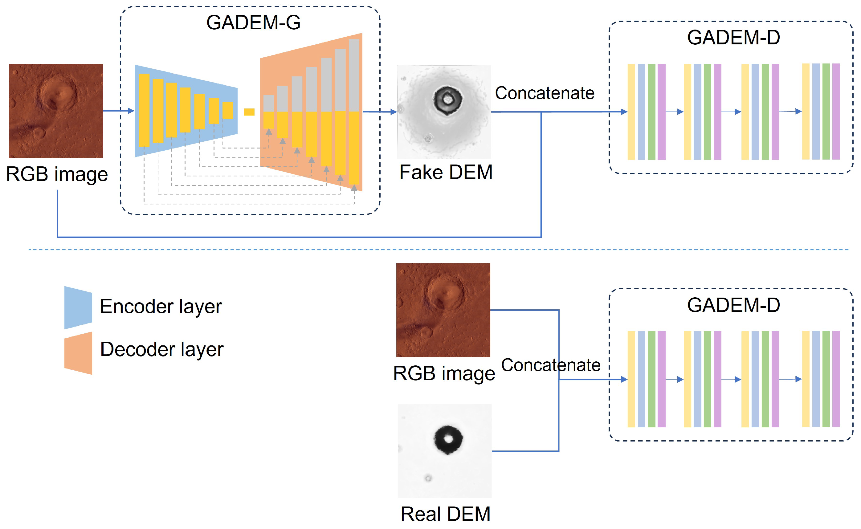
As shown in Figure 1, GADEM consists of a generator network named GADEM-G and a discriminator network named GADEM-D.

Figure 1.
The entire process of GADEM.
The goal of the GADEM-G is to convert an input RGB image into a synthetic DEM image that visually resembles a real DEM. This process involves passing the input RGB image through a neural network architecture consisting of an encoder and a decoder. The encoder compresses the RGB image into a latent representation, and the decoder reconstructs this representation into a DEM image. The purpose of GADEM-D is to distinguish the generated DEMs and real DEMs. During the training phase, a series of games are played between GADEM-G and GADEM-D, in which GADEM tries to generate more and more realistic DEM images, while GADEM-D strives to improve its ability to distinguish fake DEMs from real DEMs. Through this confrontation process, GADEM-G gradually learns how to generate high-quality DEM data, and GADEM-D becomes good at detecting generated images that are different from real DEMs. Ultimately, our network is able to generate trustworthy DEMs from RGB images.
3.2. GADEM Network Structure
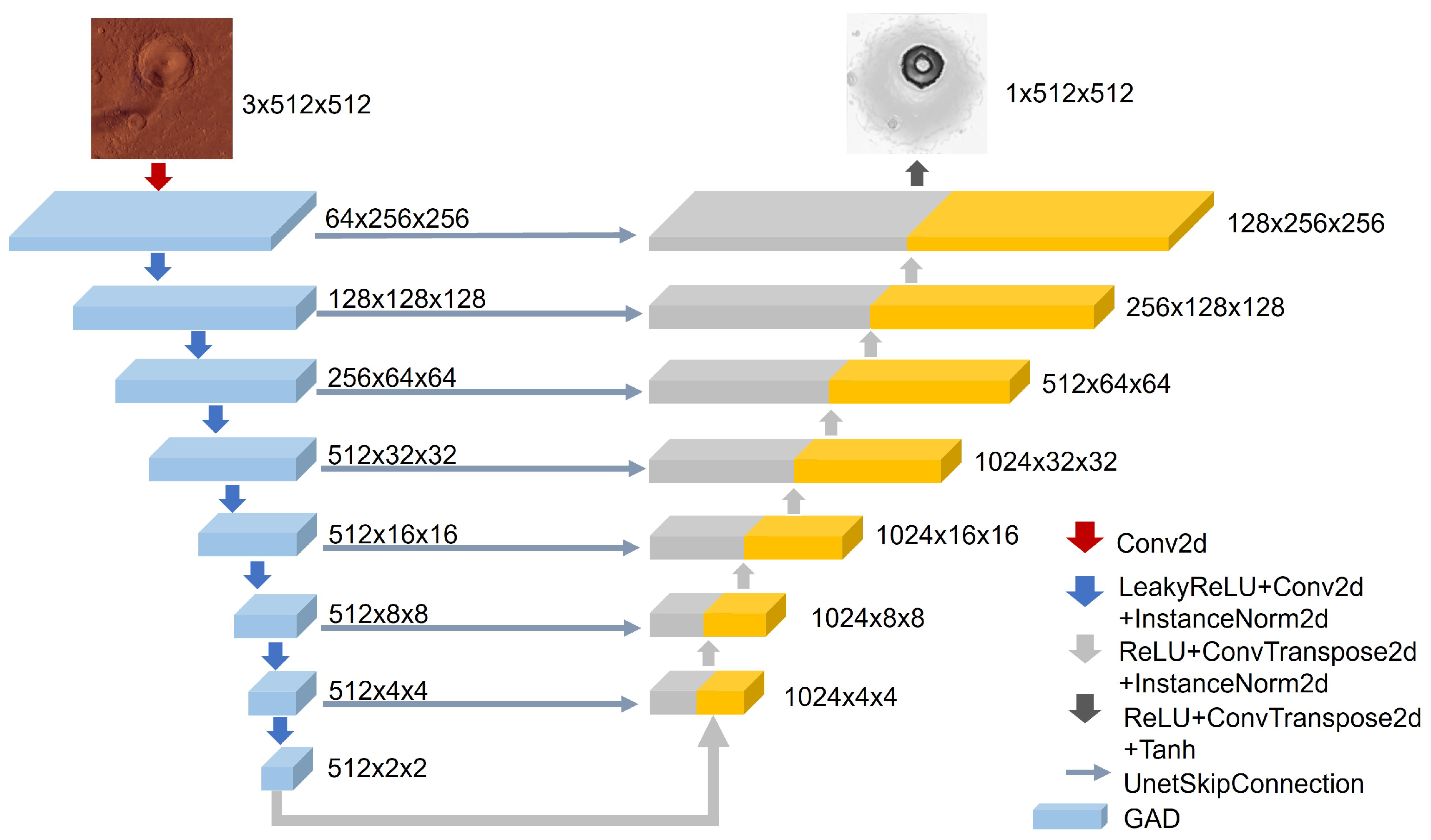
The generator of GADEM employs an encoder–decoder structure, as shown in Figure 2. This structure incorporates jump connections to achieve effective integration of local and global information. In the encoder stage, the input RGB image is first processed by GAD for feature extraction, followed immediately by a downsampling operation to reduce the spatial resolution while increasing the depth of the features to capture the key information in the image. The decoder employs an inverse strategy, where it progressively upsamples the feature map to recover its spatial dimensions using inverse convolutional layers. The ReLU activation function and the InstanceNorm2d layer follow the ConvTranspose2d layer. In this process, the jump connections in the GADEM-G architecture pass the feature maps of each stage from the encoder directly to the corresponding layer in the decoder. This operation can maintain the integrity of the feature information. After passing through multiple upsampling stages of the decoder, the final output is generated through another inverse convolutional layer and normalized by the Tanh activation function to ensure that the reconstructed DEM matches the original input image in resolution.
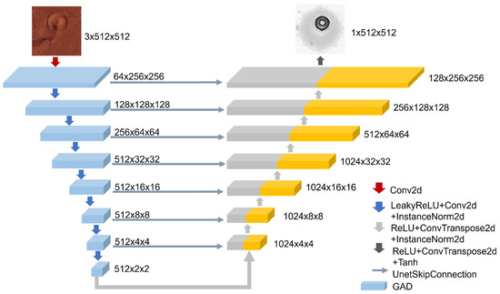
Figure 2.
Network architecture of GADEM-G.
Figure 3 illustrates our discriminator network GADEM-D. Its network structure is similar to PatchGAN [9], consisting of a series of convolutional layers. The network takes as input a combined image of the DEM and the corresponding satellite imagery, which is subjected to successive convolutional layers, a GAM layer, a normalization layer (Layer Normalization), and a LeakyReLU activation function, ultimately resulting in a single-channel 62 × 62 feature map. This feature map represents the results of the network’s classification of the input image, where each feature unit contains discriminative information about the corresponding local region. The construction of the entire discriminator network ensures that features from different regions can be efficiently captured and analyzed to accurately assess the degree of similarity between the generated image and the real image.
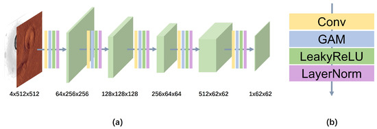
Figure 3.
Network architecture of GADEM-D. (a) Network architecture. (b) The hierarchical structure between each feature map.
3.3. GAD
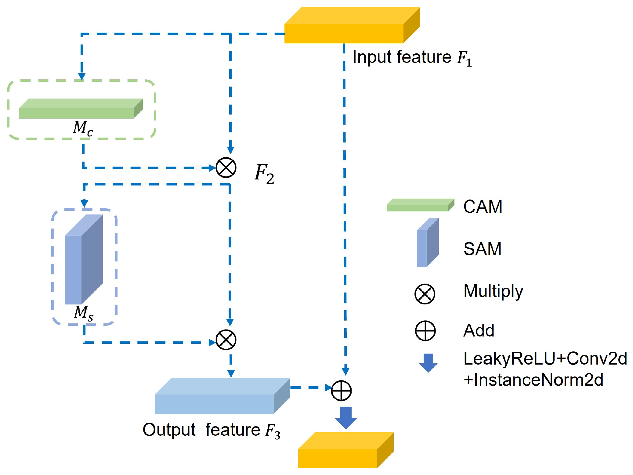
The specific structure of the GAD module in the GADEM generator network is shown in Figure 4. GAD mainly includes two sub-modules: channel attention module and spatial attention module. Given the input feature map , firstly, the channel attention sub-module’s output is multiplied by the original feature map to obtain the intermediate feature , as shown in what follows:
where is the channel attention sub-module and ⊗ represents elementwise multiplication. The intermediate feature is input to the spatial attention sub-module, and its output result is multiplied with to obtain the output result , as shown in what follows:
where is the spatial attention sub-module. and are added to obtain the final output feature.
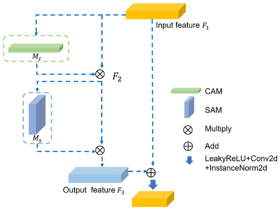
Figure 4.
Network architecture of GAD.
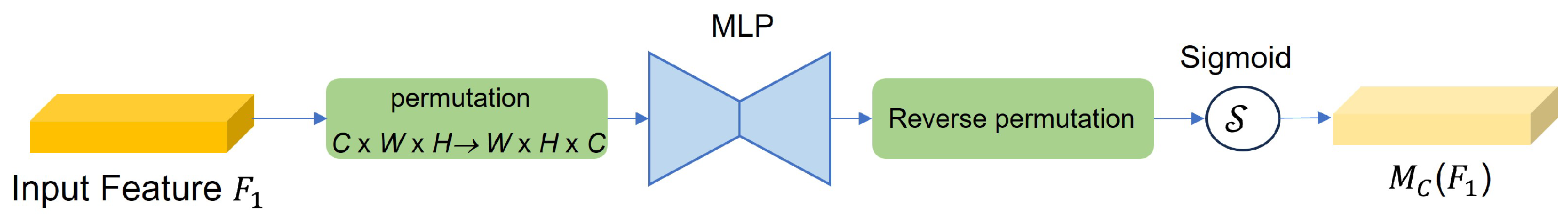
The CAM is shown in Figure 5. In the CAM, the input features are first subjected to a permutation transformation, adjusting their dimensions from C × W × H to W × H × C. Then, a multi-layer perceptron (MLP) with a reduction ratio of r is used for dimensionality reduction. The MLP follows the encoder–decoder structural design and learns the complex dependencies between different channels. The output is returned to the original dimension through inverse permutation, and then, the channel attention map is obtained through the Sigmoid function.
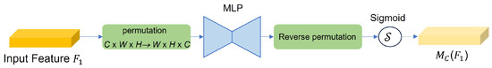
Figure 5.
Network architecture of CAM.
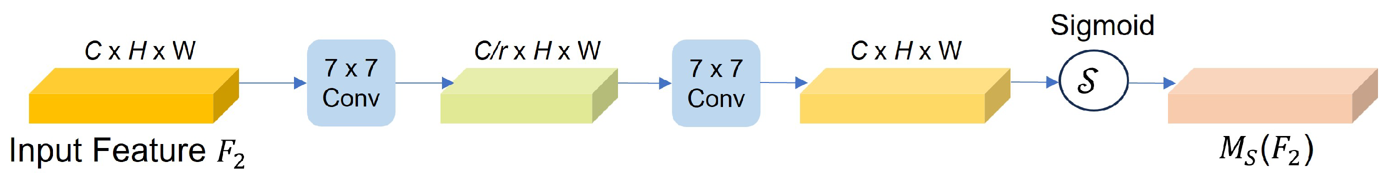
The SAM is shown in Figure 6. This module uses two convolutional layers and adopts the same reduction rate r as the CAM. In addition, in order to avoid the loss of feature information, the SAM deletes the pooling layer to retain more key features.
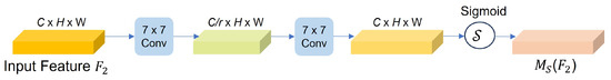
Figure 6.
Network architecture of SAM.
The SAM is similar to SENet [23]. First, the feature map reduces the number of channels through convolution with a kernel size of 7 to reduce the computational cost. Then, a convolution operation with a kernel size of 7 is performed to increase the number of channels and keep the number of channels consistent. Finally, the feature map is processed by the Sigmoid function to obtain the output.
3.4. Multi-Order Gradient Fusion Loss Function
When dealing with weakly textured images such as the lunar surface, traditional pixel-level loss functions, such as the L1 or L2 loss, often struggle to capture subtle terrain variations. Gradient refers to the rate of change of pixel intensity in an image, which quantifies the difference in intensity between each pixel and its surroundings. Gradient loss can provide richer information about image variations, especially in regions where texture is not obvious. Considering the high sensitivity of DEM to edges and texture details, the introduction of gradient loss can enhance the network’s ability to recover key features such as edges and texture details. The gradient loss function highlights the edge and texture information of an image by quantifying the intensity variations between neighboring pixels in the image. Therefore, the loss function can be expressed as:
where represents the pair loss part of the conditional adversarial network. The generator attempts to generate data that are realistic enough to “fool” the discriminator, while the discriminator’s goal is to distinguish between the generated data and real data. is the L1 loss, which encourages the generator to generate images that are close to the real data at the pixel level. It is the sum of the absolute values of the pixel value differences between the generated image and the real image. and represent the first-order gradient loss and the second-order gradient loss, respectively. , , and are weight coefficients, where the value of is the same as in Pix2Pix, set to 100. The weights of and are assigned based on the experimental effects. The first-order difference focuses on capturing edge and line features in elevation maps to more accurately depict the fine structure of the terrain and improve the visual quality of the image. The first-order gradient loss is defined as follows:
where is the first-order gradient loss in the vertical direction and is the first-order gradient loss in the horizontal direction. The formulas are as shown in what follows, respectively:
where and represent the height values of the predicted image and the real image at position , respectively, N represents the resolution in the y direction, M represents the resolution in the x direction, and ∇ represents backward differentiation.
The second-order difference is particularly sensitive to small texture and detail changes in the image, making the depth of the crater more prominent. The second-order gradient loss is:
where is the second-order gradient loss in the vertical direction and is the second-order gradient loss in the horizontal direction. The specific calculation formulas are as shown in what follows:
where represents the second-order difference.
4. Experiments
In order to verify the effectiveness of the proposed algorithm, we constructed the Moon and Mars datasets as typical planetary surfaces to verify the accuracy of the algorithm. This section first introduces how to construct datasets from public planetary images, then introduces the experimental methods and evaluation metrics. Finally, we conducted the experiments and analyzed the results.
4.1. Construction of Datasets
We created the dataset using public low-resolution data of Mars and the Moon based on the Lunar Orbiter Laser Altimeter provided by the National Aeronautics and Space Administration (NASA) [37] and high-resolution data of the Moon’s South Pole obtained by China’s Chang’e 2 [38]. As shown in Figure 7, elevations were computed by subtracting the lunar reference radius of 1737.4 km from the surface radius measurements, and the resolution of the planet surface DEM in TIFF format and the planet surface image in PNG format is 463m/pixel. Among these, Figure 7a is the surface RGB data of the Moon and Figure 7b is the corresponding DEM data. Figure 7c,d show RGB data and DEM data on the surface of Mars. From the data of the Lunar South Pole shown in Figure 8, its DEM resolution reaches 20 m/pixel, which was produced using images acquired by the Chang’e-2 stereo camera CCD at an orbital altitude of 100 km.
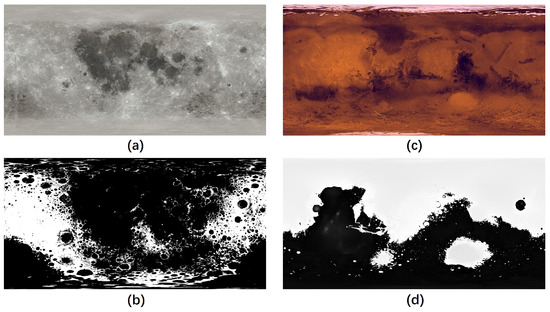
Figure 7.
Source satellite images of Mars and the Moon and their DEM data. The number of pixels of (a) is 27,360 × 13,680, (b) is 23,040 × 11,520, (c) is 46,080 × 23,040, and (d) is 46,080 × 23,040.
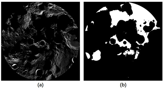
Figure 8.
The data captured by the Chang’e-2 CCD camera were selected from the block of 87 degrees south latitude and 0 degrees west longitude. The image resolution is 18,363 × 18,363. Among these, (a) and (b) represent the RGB and DEM data of the block respectively.
As can be seen, the resolutions of the lunar satellite image and the corresponding DEM do not match. To overcome these challenges, we performed a series of image-processing steps. First, we downsampled the lunar satellite image using nearest interpolation methods [39] to a uniform resolution and mapped the DEM to a grayscale image with elevation values of 0–255. Second, we minimized the matching error through two stages of coarse and fine registration. We applied the Sobel operator with a 3 × 3 convolution kernel in the horizontal and vertical directions to perform multiple rounds of edge detection on the RGB image and the DEM grayscale image, searching for the best pixel offset within a predefined large range. In the coarse registration stage, the threshold of the Sobel operator was set to a range of −50 to 50 pixels to limit the search interval and quickly determine the best initial offset. The RGB data were then re-cropped from the original image based on this preliminary offset. In the subsequent fine registration stage, the Sobel calculation was continued on the cropped RGB data and the grayscale image, and the threshold range of the Sobel operator was narrowed to 3 pixels. Several iterations of the search loop were performed to ensure accurate alignment. For Mars data of the same resolution, we also performed two stages of alignment work.
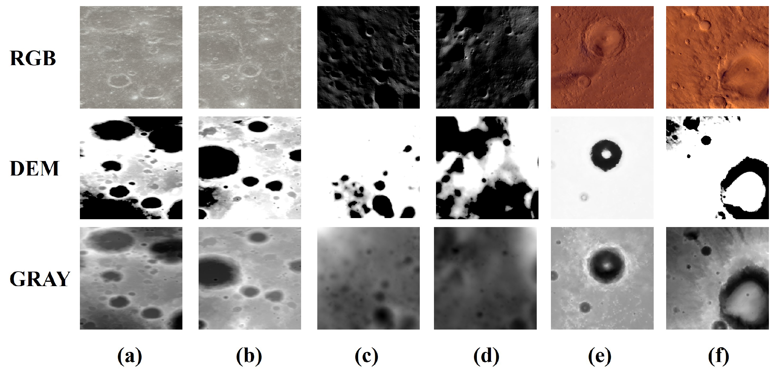
To accommodate the varied terrain heights of different planets within a unified model, we have undertaken a series of normalization processes on the elevation values present in the imagery. Initially, elevation values were adjusted to a more suitable range of −5 to 15 m to better align with the requirements of the training model. In addition, in order to reduce the error caused by invalid images, we eliminated images in the polar region from the NASA data. To bolster the network model’s robustness, rotation and flipping techniques were employed as methods of data augmentation. The aligned and normalized image data were subsequently cut into smaller patches of 512 × 512 pixels. The resulting datasets include 5299 images for Mars, where 4239 images were for training and 1060 images for testing. There were 3378 images for the lunar surface, where 3049 images were for training and 338 images for testing. For the Lunar South Polar shadow region data, we produced 2426 images for training and 270 images for testing in the region of S, W. Figure 9 shows the aligned RGB images and the DEM in TIFF format, together with the grayscale images used as a reference for alignment.

Figure 9.
(a,b) are lunar data; (c,d) are Mars data; (e,f) are Lunar South Pole data. Gray represents grayscale images.
4.2. Evaluation Metrics
To comprehensively evaluate the effectiveness of our method, we adopted both objective metrics and a qualitative evaluation [40]. In our experiments, we converted the generated DEM into a 3D representation for visualization and judged the quality of DEM generation through qualitative evaluation of this visualization.
Objective metrics include a series of rating metrics. Among these, the mean average error (MAE) and the mean-squared error (RMSE) evaluate the overall generation error and are defined in Equations (10) and (11):
where represents the height value of the original image and represents the predicted height value. Further considering the structure of the image itself, the fitting superiority (R²) and Structural Similarity Index Measure (SSIM) were used to evaluate the reconstruction degree of the model. The calculation equation is as follows:
where represents the mean height of the original image.
where and represent the global average height of the real image and the generated image, respectively, and and are the global variance of the real image and the generated image, indicating the degree of dispersion of height values. is the covariance between the real image and the generated image, representing the similarity of the height values between the two images. and are constants used to avoid a denominator of 0. Here, is set to 0.0225 and is set to 0.2025.
Secondly, we evaluated the similarity between the reconstructed DEM and the original image from a subjective visual perspective through the generated grayscale image and the OBJ model converted from the TIFF data.
4.3. Experimental Plan
We used an Intel i9-9820X CPU and NVIDIA GeForce RTX 3090 GPU for model training. The epochs were set to 400, the learning rate to 0.002, and the batch size to 16, and the optimizer was Adam. The baseline network we used was Pix2Pix [5]. In order to compare the effect of the attention mechanism on terrain generation, we chose CBAM for comparison, which is named CBDEM. Secondly, we set and in the loss function to 10.
4.4. Experimental Results
We mixed Moon and Mars data from NASA for training and evaluated the respective test dataset, then compared the metrics of each model, as shown in Table 1. The proposed GADEM significantly outperformed the CBDEM algorithm on multiple key performance metrics. Specifically, on the lunar dataset, our GADEM algorithm was 17.67% and 35.13% higher than the CBDEM algorithm in the R2 and SSIM metrics, respectively. Similarly, on the Mars dataset, GADEM’s improvements in these two metrics reached 37.84% and 28.66%, respectively.

Table 1.
Performance comparison of terrain-generation algorithms on lunar and Mars datasets.
This significant advantage is partly due to the difference in processing strategies between the two algorithms. The CBDEM algorithm focuses more on the reconstruction of local terrain, while the GADEM algorithm focuses on the reconstruction of global terrain. Therefore, although the improvement of our method compared to the CBDEM algorithm is not particularly large in terms of error metrics, under the design of comprehensive multi-order gradient loss, GADEM shows superior performance in terms of the similarity of the overall structure of the terrain; thus, it demonstrates its significant advantages in global terrain reconstruction.
It was also observed that, among the comparison algorithms, the CBDEM algorithm has better performance metrics than the Pix2Pix algorithm. On the lunar dataset, the MAE and RMSE of CBDEM were 13.67% and 17.12% lower than Pix2Pix, respectively, and the R2 and SSIM were 57.83% and 57.28% higher, respectively. On the Mars dataset, CBDEM was 18.79% lower than Pix2Pix in the MAE, 23.28% lower in the RMSE, 79.17% higher in the R2, and 62.62% higher in the SSIM, indicating that CBDEM has certain performance improvements in image structure and quality reconstruction. CBDEM also had similar performance advantages on the Mars dataset. This is because CBDEM structurally introduces spatial and channel attention relative to Pix2Pix. Spatial attention can help the model focus on specific areas of the image, while channel attention enables the model to highlight more important feature channels.
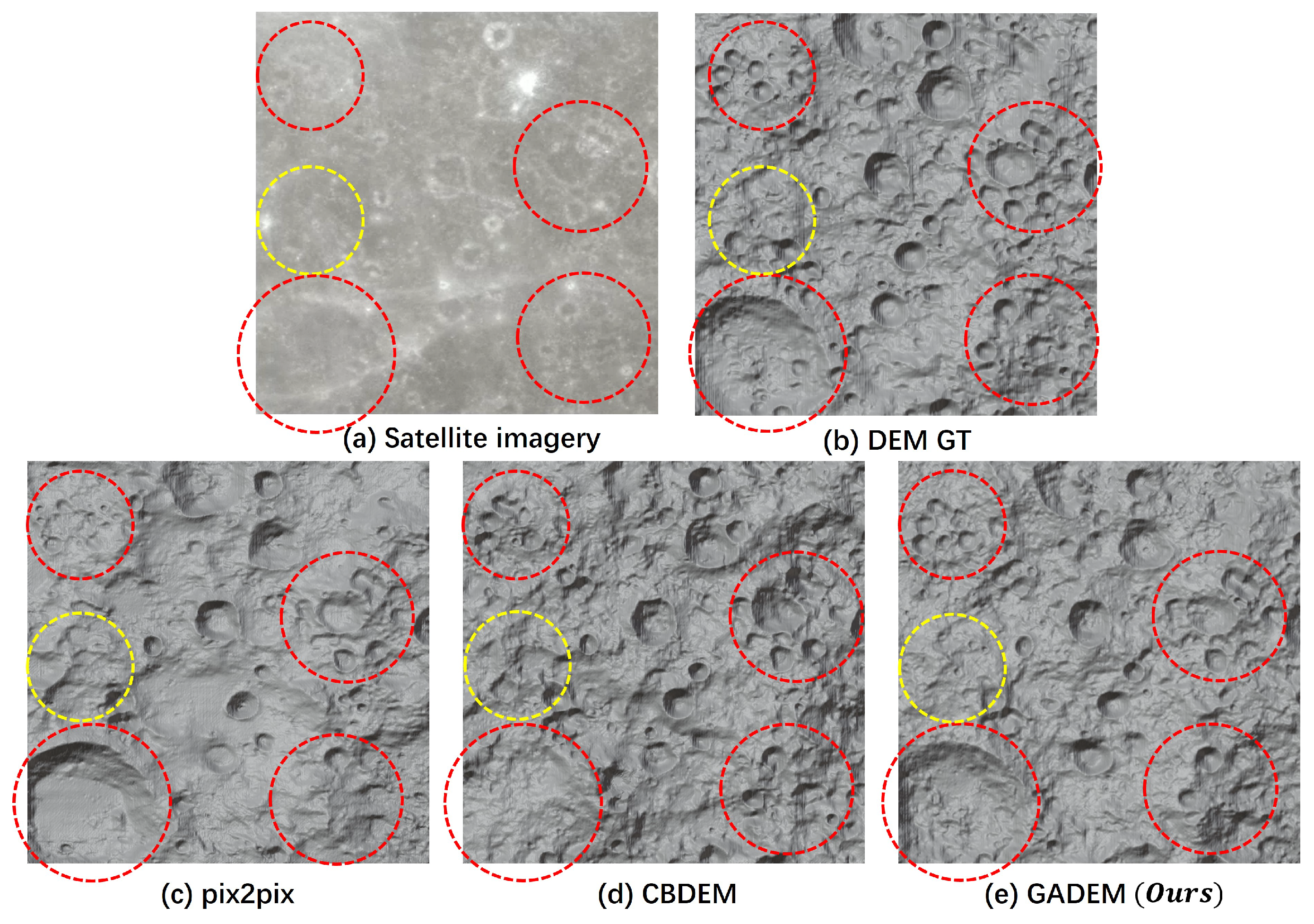
We converted the generated DEM model into a three-dimensional model in OBJ format and evaluated the effect from a visual perspective from a top-down perspective, as shown in Figure 10 and Figure 11. The red circles indicate the area where our proposed model outperforms other models, while the yellow ones are the opposite. Among these, satellite imagery represents the input, DEM GT represents the real DEM corresponding to the satellite image, and the remaining pictures displayed are the effects generated by various models. Our network specifies that the generated DEM is 512*512, with 512 meshes in both horizontal and vertical directions. Since the Mars and Moon data we downloaded are from NASA and their DEM resolution is 463 m, within the same 512*512 range, the Moon surface will show more dense crater features, while the Mars DEM will show sparsely distributed craters.
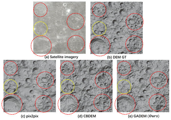
Figure 10.
Comparison of the generation of mountain and crater terrain in the lunar datasets.
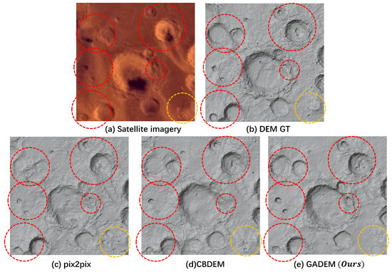
Figure 11.
Comparison of the generation of mountain and crater terrain in the Mars datasets.
Through comparative analysis of the terrain reconstruction effect in the provided images, we observed that the proposed GADEM has significantly improved effects compared to Pix2Pix and CBDEM. Especially in the area marked by the red circle, its reconstruction effect is highly consistent with the DEM GT, proving its excellent performance in the synthesis of global terrain features. In addition, the GADEM algorithm also significantly outperforms the other two methods in the overall quality of the generated images, including light and dark contrast and layered details, which strengthens its advanced performance and practical value in complex-terrain-reconstruction tasks. Compared with the comparison algorithm, the DEM generated by the Pix2Pix method appears blurry in terms of edge processing. This is especially obvious in the area marked by the red circle in the figure. There is a large deviation between the reconstructed details and the DEM GT. CBDEM shows finer reconstruction capabilities in these key areas, but compared to our proposed algorithm, the details are still insufficient.
In the yellow circled part of the satellite image, the proposed GADEM algorithm resulted in a smoother result. It can be seen from the corresponding RGB image that the terrain features in this area are not obvious and the pixel changes are subtle, making it difficult to identify the specific terrain. Our GADEM algorithm produces smoother results in these difficult-to-identify areas due to its emphasis on global terrain reconstruction.
4.5. Terrain Profile Analysis
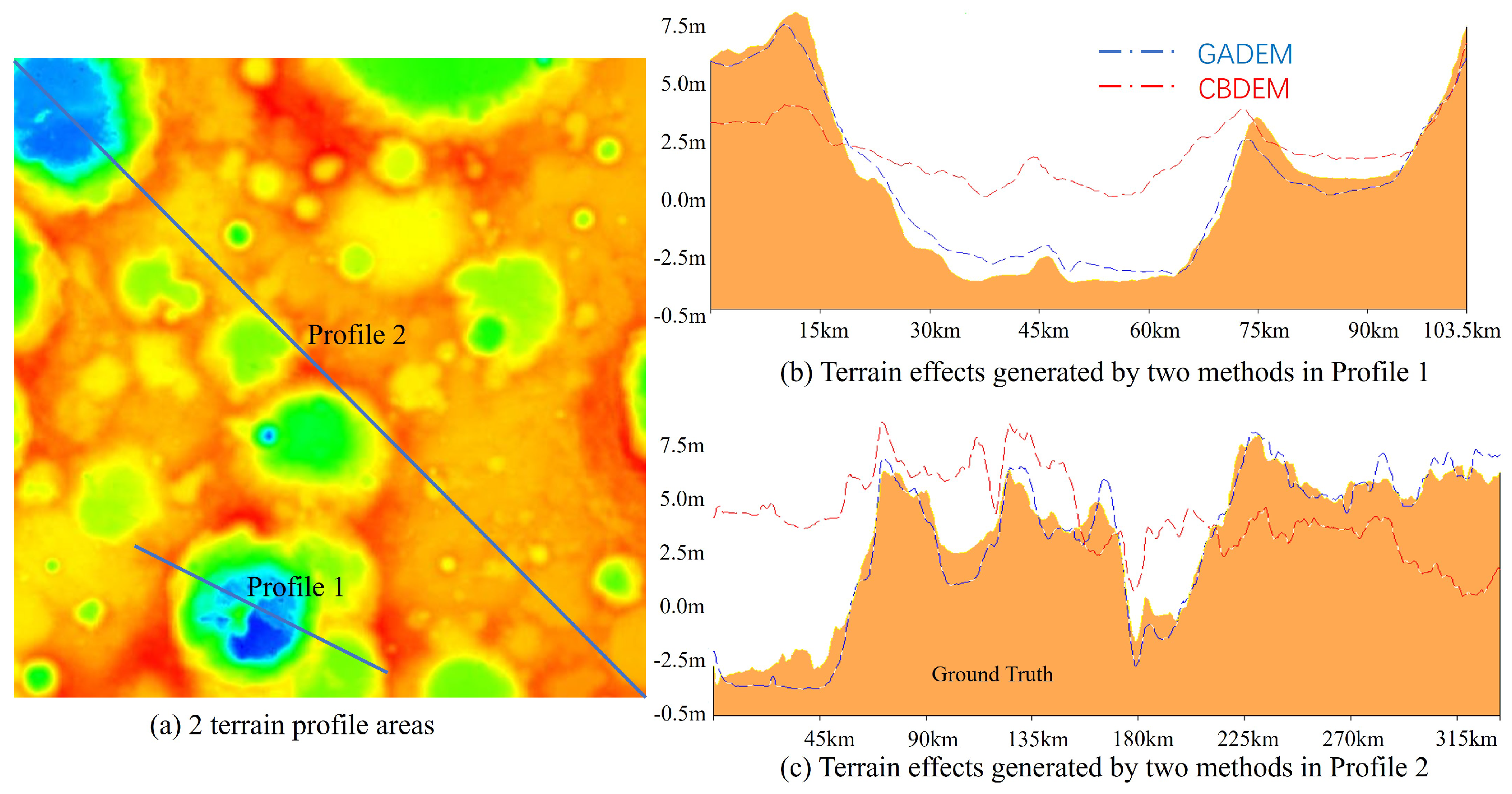
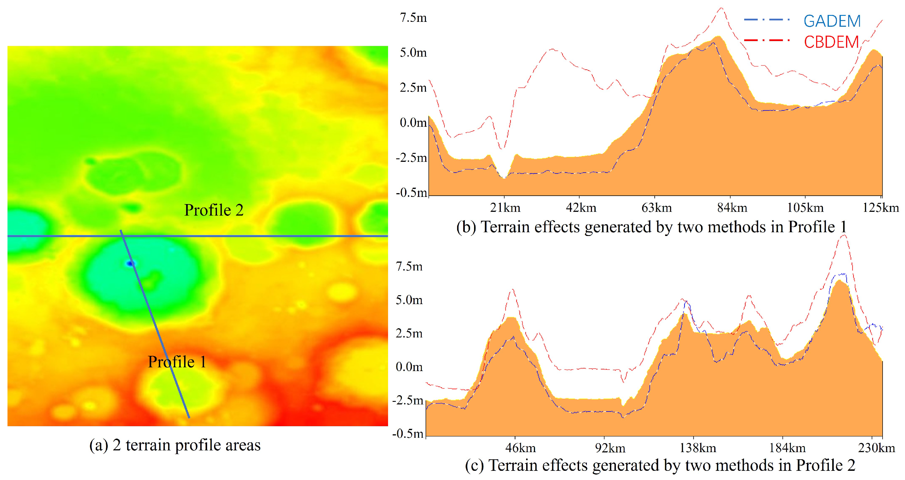
In order to more intuitively illustrate the advantages of the proposed algorithm in DEM reconstruction, a comparative analysis of multiple lunar surface terrain profiles was conducted, as shown in Figure 12 and Figure 13. We selected terrain profiles of dense crater areas and sparse crater areas for comparison. The significant changes in the lunar surface presented by these terrains provide an ideal scenario for verifying the effectiveness of this research method.
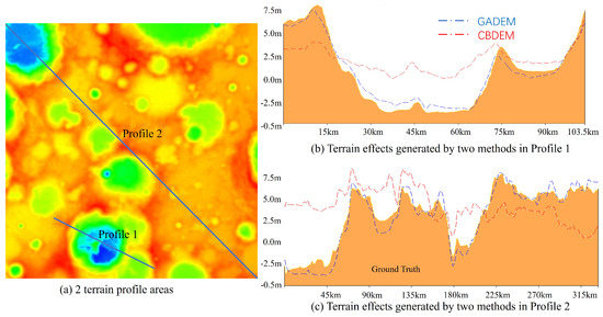
Figure 12.
Comparison of GADEM and CBDEM methods in dense crater terrain profile analysis.

Figure 13.
Comparison of GADEM and CBDEM methods in sparse crater terrain profile analysis.
CBDEM is able to preserve detailed morphological features of local craters, especially in densely cratered areas. This advantage is attributed to its local nature, which allows it to focus on smaller areas. Although GADEM is less detailed in terms of small-scale features, it can more accurately reconstruct global topography. It provides a more comprehensive and accurate representation of the lunar surface compared to CBDEM. CBDEM has significant deviations compared to real lunar topographic data, especially in the magnitude of slope undulations and overall height trends. These differences indicate that, although CBDEM can capture local details, it may introduce errors when extended to larger areas. This limitation highlights the need for careful consideration when applying CBDEM to a wide range of topographic reconstruction tasks.
4.6. Shadow Region Experiment
Similarly, we tested on the Lunar South Pole data and found that GADEM’s ability to generate a lunar surface model exceeded the comparable models. As shown in Table 2 below, GADEM achieved the minimum in terms of error loss and received the highest score in terms of reconstruction similarity.
Table 2.
Performance comparison of terrain generation algorithms on Lunar South Pole dataset.
Exporting it as a 3D representation of the DEM allows for a more intuitive comparison of the generation effects of various networks. The following Figure 14 shows the visualization of the DEM in the MeshLab software v2022.02.
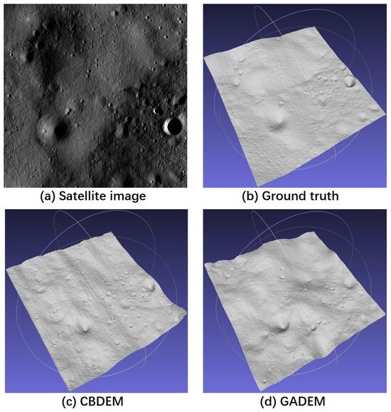
Figure 14.
Comparison of GADEM and CBDEM methods in terrain profile analysis. (a) is a cropped satellite image with a size of 512 × 512. (b) is the effect of converting the DEM corresponding to the current satellite image into 3D representation. (c,d) are the effects of converting the DEM generated by CBDEM and GADEM into a 3D representation.
The DEM generated by the CBDEM method attempts to reconstruct the complexity of the lunar surface and capture its topographic features with some degree of accuracy. In addition, CBDEM retains certain morphological details that disappear when using GADEM, demonstrating its advantages in specific terrain reconstructions. However, CBDEM’s reproductions exhibit significant biases compared to real lunar topography data, particularly in terms of slope relief magnitude and the overall height trends characterizing the lunar surface. These differences highlight the limitations of CBDEM, whereas GADEM performs more accurately in global terrain reconstruction.
In contrast, the DEM generated by GADEM shows significant improvements over its CBDEM counterpart, although it did not perfectly generate the lunar topography. The results of the evaluation indicated that GADEM outperformed CBDEM in all evaluation metrics. However, due to the image pixels in the shadow area, the GADEM method’s ability to generate terrain at the Lunar South Pole is not as good as in places without shadow areas.
4.7. Ablation Experiment
In this section, we will analyze the effectiveness of GAD and multi-order gradient loss. Likewise, we analyzed this both objectively and subjectively. Table 3 shows the effect of GAD and multi-order gradient loss in the GADEM algorithm, where w/o means that the module or the gradient loss is not included and w means that the module or the gradient loss is included. In the GAD experiment, GradLoss was not included, and similarly, GAD was not included in the GradLoss experiment.
Table 3.
Comparative evaluation of algorithms with GAD module and multi-stage gradient loss on lunar and Martian terrain datasets.
For the lunar dataset, the introduction of the GAD module resulted in a reduction of the MAE from 2.978 m to 2.617 m, a decrease in the RMSE from 3.165 m to 2.856 m, an increase in the R² from 0.351 to 0.459, and an improvement in the SSIM from 0.316 to 0.409. Similarly, for the Mars dataset, the GAD module demonstrated the same level of optimization enhancement. These findings indicate that the GAD module significantly contributes to the precision of terrain reconstruction.
Upon further investigation of the GradLoss effect, it was observed that the employment of a singular gradient loss further enhances the reconstructed error metric compared to using the GAD module alone. As GAD is more focused on global effects, the gradient loss does not enhance the reconstruction index as effectively as when the GAD module is used independently. On the lunar dataset, with the application of , the MAE and RMSE were reduced to 2.513 m and 2.581 m, respectively. With the application of , the MAE decreased to 2.525 m, the RMSE to 2.634 m, and the R² and SSIM were recorded at 0.417 and 0.432, respectively. Moreover, it was found that the surpassed in terms of the error index, while the reconstruction degree index for was higher than that of . These outcomes highlight the distinct contributions of and in various dimensions, enhances the accuracy of terrain contours, whereas shows superior performance in fitting terrain elevations.
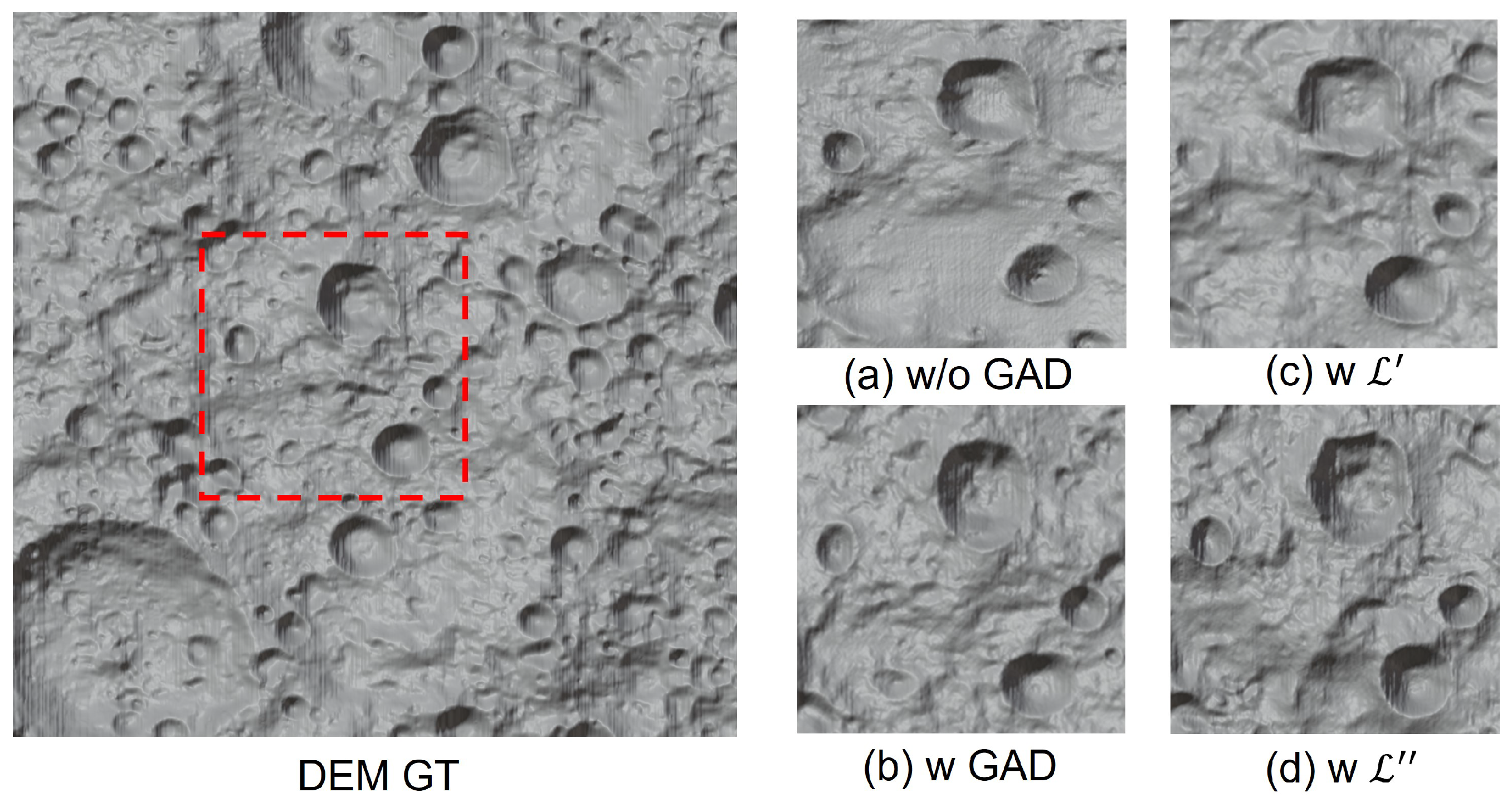
As illustrated in Figure 15 and Figure 16, the results of our DEM generation for each module are presented in a three-dimensional model format. Here, the terrain within the red dotted box in the DEM GT is evaluated.
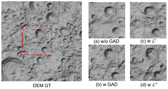
Figure 15.
Results generated from lunar data in various ablation experiments.
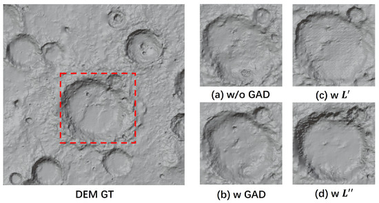
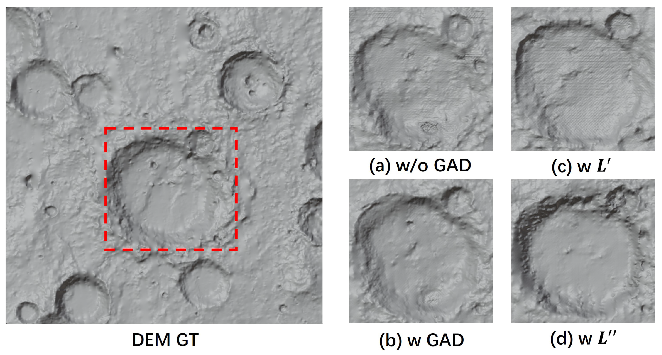
Figure 16.
Results generated from Mars data in various ablation experiments.
In the absence of GAD module support, the DEM terrain reconstruction results shown in Figure 15 and Figure 16 significantly differ from the DEM Ground Truth (GT) in terms of edge details and overall terrain characteristics. Features within the red dotted box appear quite vague, failing to clearly demonstrate the terrain’s fine structure. Conversely, in configurations utilizing the GAD module, the reconstruction results demonstrate a higher consistency in global structure and terrain features, effectively showcasing the GAD module’s efficacy in overall terrain reconstruction. Additionally, the introduction of the GAD module not only enhances the clarity of terrain edges, but also plays a crucial role in capturing subtle terrain variations, thus providing a more accurate visual basis for understanding and analyzing terrain.
Secondly, the results utilizing exhibit better terrain contours and details, particularly around the edges and internal structures of craters, making these areas more closely resemble the actual terrain. The application of further enhances the accuracy of terrain height details. Although slightly less sharp in terms of contour definition compared to , it outperforms in terrain height fitting. Moreover, the results displayed in the figures also confirm the reliability of the data presented in Table 3. Notably, uniquely excels in addressing minor variations in terrain height, allowing the model to capture the terrain’s microscopic changes more delicately, thereby offering a richer set of information for terrain analysis.
Overall, these image results reveal the independent and complementary roles of the GAD module and gradient loss in the task of terrain reconstruction. excels in depicting terrain contours, while demonstrates advantages in capturing height change details. The introduction of the GAD module significantly enhances the global consistency of reconstruction results, strengthening the model’s grasp on the global structure and features of the terrain. Therefore, our GADEM algorithm comprehensively considers the synergistic effect of different modules and loss functions to achieve the best reconstruction effect.
5. Conclusions and Future Work
In this comprehensive study, we introduced the GADEM network, a pioneering approach for the reconstruction of DEMs of planetary surfaces utilizing satellite imagery. The core innovation of the GADEM network lies in its integration of the GAD module, which leverages attention mechanisms across both the channel and spatial dimensions to significantly enhance the network’s capability in accurately reconstructing global crater topographies. This integration not only elevates the model’s overall performance, but also broadens its applicability in planetary science.
A distinctive feature of the GADEM network is its employment of a multi-order loss function. This sophisticated approach synergizes first-order and second-order gradient losses, markedly boosting the network’s proficiency in capturing intricate details during DEM generation. This methodological advancement represents a significant leap forward in the accuracy and detail of topographical reconstruction from satellite data.
To validate the effectiveness of the GADEM network, we meticulously curated datasets for both the Moon and Mars. These datasets address and correct the prevalent mismatch issues between existing satellite imagery and DEM data, providing a robust foundation for our experiments. By selecting a diverse array of terrain samples, we have conducted extensive tests that underscore the practical utility and effectiveness of our proposed method in real-world scenarios.
Looking ahead, our future endeavors will focus on the topographic reconstructions of the Lunar South Pole’s Permanent Shadow Regions (PSRs), because the water ice contained in these areas is of great scientific significance to future human migration to alien planets. However, these areas are almost completely dark from satellite images, blurring the details of the terrain, and directly reconstructing 3D models of these areas through software faces huge challenges. To overcome these obstacles, we will incorporate an analysis of the lunar geological environment, taking into account various geological features such as crater rim height and diameter, as well as solar altitude angle. Our methodology will blend the latest advancements in Artificial Intelligence and Generative Content (AIGC) technologies to reconstruct the topography of these shadowed regions as accurately as possible. This effort is not just academic; understanding the geology of lunar polar regions is crucial for future lunar exploration and the potential utilization of lunar resources, paving the way for groundbreaking discoveries and advancements in planetary science [41,42,43].
Author Contributions
Conceptualization, Z.Z., L.Y. and L.S.; methodology, Z.Z., L.Y. and L.S.; software, Z.Z., L.Y. and L.S.; validation, Z.Z., L.Y. and L.S.; formal analysis, Z.Z., L.Y. and L.S.; investigation, Z.Z., L.Y. and L.S.; resources, L.Y., L.Y. and L.S.; data curation, Z.Z., L.Y. and L.S.; writing—original draft preparation, Z.Z., L.Y. and L.S.; writing—review and editing, Z.Z., L.Y. and L.S.; visualization, Z.Z., L.Y. and L.S.; supervision, L.Y., L.S. and D.Z.; project administration, L.Y., L.S. and D.Z.; funding acquisition, L.Y., L.S. and D.Z. All authors have read and agreed to the published version of the manuscript.
Funding
This work was supported by the National Natural Science Foundation of China under grant 52372423 and “Pioneer” and “Leading Goose” R&D Program of Zhejiang (grant number 2024C01028).
Institutional Review Board Statement
Not applicable.
Informed Consent Statement
Not applicable.
Data Availability Statement
The data that support the findings of this study are openly available at https://svs.gsfc.nasa.gov/ (accessed on 1 September 2023) and http://moon.bao.ac.cn (accessed on 1 September 2023).
Conflicts of Interest
The authors declare no conflicts of interest.
References
- Hu, R.; Zhang, Y. Fast path planning for long-range planetary roving based on a hierarchical framework and deep reinforcement learning. Aerospace 2022, 9, 101. [Google Scholar] [CrossRef]
- Hong, Z.; Sun, P.; Tong, X.; Pan, H.; Zhou, R.; Zhang, Y.; Han, Y.; Wang, J.; Yang, S.; Xu, L. Improved A-Star algorithm for long-distance off-road path planning using terrain data map. ISPRS Int. J. Geo-Inf. 2021, 10, 785. [Google Scholar] [CrossRef]
- Xu, X.; Fu, X.; Zhao, H.; Liu, M.; Xu, A.; Ma, Y. Three-Dimensional Reconstruction and Geometric Morphology Analysis of Lunar Small Craters within the Patrol Range of the Yutu-2 Rover. Remote Sens. 2023, 15, 4251. [Google Scholar] [CrossRef]
- Beckham, C.; Pal, C. A step towards procedural terrain generation with gans. arXiv 2017, arXiv:1707.03383. [Google Scholar]
- Panagiotou, E.; Chochlakis, G.; Grammatikopoulos, L.; Charou, E. Generating elevation surface from a single RGB remotely sensed image using deep learning. Remote Sens. 2020, 12, 2002. [Google Scholar] [CrossRef]
- Yao, S.; Cheng, Y.; Yang, F.; Mozerov, M.G. A continuous digital elevation representation model for DEM super-resolution. ISPRS J. Photogramm. Remote Sens. 2024, 208, 1–13. [Google Scholar] [CrossRef]
- Chen, Z.; Wu, B.; Liu, W.C. Mars3DNet: CNN-based high-resolution 3D reconstruction of the Martian surface from single images. Remote Sens. 2021, 13, 839. [Google Scholar] [CrossRef]
- Mirza, M.; Osindero, S. Conditional generative adversarial nets. arXiv 2014, arXiv:1411.1784. [Google Scholar]
- Isola, P.; Zhu, J.Y.; Zhou, T.; Efros, A.A. Image-to-image translation with conditional adversarial networks. In Proceedings of the IEEE Conference on Computer Vision and Pattern Recognition, Honolulu, HI, USA, 21–26 July 2017; pp. 1125–1134. [Google Scholar]
- Bhushan, S.; Shean, D.; Alexandrov, O.; Henderson, S. Automated digital elevation model (DEM) generation from very-high-resolution Planet SkySat triplet stereo and video imagery. ISPRS J. Photogramm. Remote Sens. 2021, 173, 151–165. [Google Scholar] [CrossRef]
- Ghuffar, S. DEM generation from multi satellite PlanetScope imagery. Remote Sens. 2018, 10, 1462. [Google Scholar] [CrossRef]
- Tao, Y.; Muller, J.P.; Conway, S.J.; Xiong, S. Large area high-resolution 3D mapping of Oxia Planum: The landing site for the ExoMars Rosalind Franklin rover. Remote Sens. 2021, 13, 3270. [Google Scholar] [CrossRef]
- Tao, Y.; Muller, J.P.; Xiong, S.; Conway, S.J. MADNet 2.0: Pixel-Scale Topography Retrieval from Single-View Orbital Imagery of Mars Using Deep Learning. Remote Sens. 2021, 13, 4220. [Google Scholar] [CrossRef]
- Mou, L.; Zhu, X.X. IM2HEIGHT: Height estimation from single monocular imagery via fully residual convolutional-deconvolutional network. arXiv 2018, arXiv:1802.10249. [Google Scholar]
- Gao, Q.; Shen, X. StyHighNet: Semi-supervised learning height estimation from a single aerial image via unified style transferring. Sensors 2021, 21, 2272. [Google Scholar] [CrossRef]
- Lu, J.; Hu, Q. Semantic Joint Monocular Remote Sensing Image Digital Surface Model Reconstruction Based on Feature Multiplexing and Inpainting. IEEE Trans. Geosci. Remote Sens. 2022, 60, 4411015. [Google Scholar] [CrossRef]
- Alhashim, I.; Wonka, P. High quality monocular depth estimation via transfer learning. arXiv 2018, arXiv:1812.11941. [Google Scholar]
- Huang, G.; Liu, Z.; Van Der Maaten, L.; Weinberger, K.Q. Densely connected convolutional networks. In Proceedings of the IEEE Conference on Computer Vision and Pattern Recognition, Honolulu, HI, USA, 21–26 July 2017; pp. 4700–4708. [Google Scholar]
- Deng, J.; Dong, W.; Socher, R.; Li, L.J.; Li, K.; Li, F.-F. Imagenet: A large-scale hierarchical image database. In Proceedings of the 2009 IEEE Conference on Computer Vision and Pattern Recognition, Miami, FL, USA, 20–25 June 2009; pp. 248–255. [Google Scholar]
- Zhang, Y.; Li, K.; Li, K.; Wang, L.; Zhong, B.; Fu, Y. Image super-resolution using very deep residual channel attention networks. In Proceedings of the European Conference on Computer Vision (ECCV), Munich, Germany, 8–14 September 2018; pp. 286–301. [Google Scholar]
- Tootell, R.B.; Hadjikhani, N.; Hall, E.K.; Marrett, S.; Vanduffel, W.; Vaughan, J.T.; Dale, A.M. The retinotopy of visual spatial attention. Neuron 1998, 21, 1409–1422. [Google Scholar] [CrossRef] [PubMed]
- Wang, X.; Girshick, R.; Gupta, A.; He, K. Non-local neural networks. In Proceedings of the IEEE Conference on Computer Vision and Pattern Recognition, Salt Lake City, UT, USA, 18–23 June 2018; pp. 7794–7803. [Google Scholar]
- Hu, J.; Shen, L.; Sun, G. Squeeze-and-excitation networks. In Proceedings of the IEEE Conference on Computer Vision and Pattern Recognition, Salt Lake City, UT, USA, 18–23 June 2018; pp. 7132–7141. [Google Scholar]
- Woo, S.; Park, J.; Lee, J.Y.; Kweon, I.S. Cbam: Convolutional block attention module. In Proceedings of the European Conference on Computer Vision (ECCV), Munich, Germany, 8–14 September 2018; pp. 3–19. [Google Scholar]
- Park, J.; Woo, S.; Lee, J.Y.; Kweon, I.S. Bam: Bottleneck attention module. arXiv 2018, arXiv:1807.06514. [Google Scholar]
- Liu, Y.; Shao, Z.; Hoffmann, N. Global attention mechanism: Retain information to enhance channel-spatial interactions. arXiv 2021, arXiv:2112.05561. [Google Scholar]
- Zhang, J.; Zhou, Q.; Wu, J.; Wang, Y.; Wang, H.; Li, Y.; Chai, Y.; Liu, Y. A cloud detection method using convolutional neural network based on Gabor transform and attention mechanism with dark channel SubNet for remote sensing image. Remote Sens. 2020, 12, 3261. [Google Scholar] [CrossRef]
- Yu, Y.; Li, X.; Liu, F. Attention GANs: Unsupervised deep feature learning for aerial scene classification. IEEE Trans. Geosci. Remote Sens. 2019, 58, 519–531. [Google Scholar] [CrossRef]
- Gao, F.; He, Y.; Wang, J.; Hussain, A.; Zhou, H. Anchor-free convolutional network with dense attention feature aggregation for ship detection in SAR images. Remote Sens. 2020, 12, 2619. [Google Scholar] [CrossRef]
- Wang, L.; Yu, Q.; Li, X.; Zeng, H.; Zhang, H.; Gao, H. A CBAM-GAN-based method for super-resolution reconstruction of remote sensing image. IET Image Process. 2023, 18, 548–560. [Google Scholar] [CrossRef]
- Wang, W.; Tan, X.; Zhang, P.; Wang, X. A CBAM based multiscale transformer fusion approach for remote sensing image change detection. IEEE J. Sel. Top. Appl. Earth Obs. Remote Sens. 2022, 15, 6817–6825. [Google Scholar] [CrossRef]
- Ji, S.; Yu, D.; Shen, C.; Li, W.; Xu, Q. Landslide detection from an open satellite imagery and digital elevation model dataset using attention boosted convolutional neural networks. Landslides 2020, 17, 1337–1352. [Google Scholar] [CrossRef]
- Song, J.; Aouf, N.; Honvault, C. Attention-based DeepMoon for Crater Detection. In Proceedings of the CEAS EuroGNC 2022, Berlin, Germany, 3–5 May 2022. [Google Scholar]
- Li, W.; Wu, J.; Chen, H.; Wang, Y.; Jia, Y.; Gui, G. Unet combined with attention mechanism method for extracting flood submerged range. IEEE J. Sel. Top. Appl. Earth Obs. Remote Sens. 2022, 15, 6588–6597. [Google Scholar] [CrossRef]
- Li, Q.; Yan, D.; Wu, W. Remote sensing image scene classification based on global self-attention module. Remote Sens. 2021, 13, 4542. [Google Scholar] [CrossRef]
- Zhou, G.; Song, B.; Liang, P.; Xu, J.; Yue, T. Voids filling of DEM with multiattention generative adversarial network model. Remote Sens. 2022, 14, 1206. [Google Scholar] [CrossRef]
- Available online: https://svs.gsfc.nasa.gov/ (accessed on 1 September 2023).
- Available online: http://moon.bao.ac.cn (accessed on 1 September 2023).
- Rukundo, O.; Cao, H. Nearest neighbor value interpolation. arXiv 2012, arXiv:1211.1768. [Google Scholar]
- Polidori, L.; El Hage, M. Digital elevation model quality assessment methods: A critical review. Remote Sens. 2020, 12, 3522. [Google Scholar] [CrossRef]
- Flahaut, J.; Carpenter, J.; Williams, J.P.; Anand, M.; Crawford, I.; van Westrenen, W.; Füri, E.; Xiao, L.; Zhao, S. Regions of interest (ROI) for future exploration missions to the lunar South Pole. Planet. Space Sci. 2020, 180, 104750. [Google Scholar] [CrossRef]
- Hu, T.; Yang, Z.; Li, M.; van der Bogert, C.H.; Kang, Z.; Xu, X.; Hiesinger, H. Possible sites for a Chinese International Lunar Research Station in the Lunar South Polar Region. Planet. Space Sci. 2023, 227, 105623. [Google Scholar] [CrossRef]
- Barker, M.K.; Mazarico, E.; Neumann, G.A.; Smith, D.E.; Zuber, M.T.; Head, J.W. Improved LOLA elevation maps for south pole landing sites: Error estimates and their impact on illumination conditions. Planet. Space Sci. 2021, 203, 105119. [Google Scholar] [CrossRef]


Disclaimer/Publisher’s Note: The statements, opinions and data contained in all publications are solely those of the individual author(s) and contributor(s) and not of MDPI and/or the editor(s). MDPI and/or the editor(s) disclaim responsibility for any injury to people or property resulting from any ideas, methods, instructions or products referred to in the content. |
© 2024 by the authors. Licensee MDPI, Basel, Switzerland. This article is an open access article distributed under the terms and conditions of the Creative Commons Attribution (CC BY) license (https://creativecommons.org/licenses/by/4.0/).