Article

Precise Modeling and Analysis of Aviation Power System Reliability via the Aviation Power System Reliability Probability Network Model

1
School of Mechanical and Precision Instrument Engineering, Xi’an University of Technology, Xi’an 710048, China
2
Xi’an Institute of Optics and Precision Mechanics (XIOPM), Chinese Academy of Sciences, Xi’an 710119, China
3
College of Civil Aviation, Northwestern Polytechnical University, Xi’an 710072, China
*
Author to whom correspondence should be addressed.
Aerospace 2024, 11(7), 530; https://doi.org/10.3390/aerospace11070530
Submission received: 20 May 2024 / Revised: 19 June 2024 / Accepted: 24 June 2024 / Published: 28 June 2024

Abstract

:
This study addresses the challenges of accurately analyzing the reliability of aviation power systems (APS) using traditional models by introducing the Aviation Power System Reliability Probability Network Model (APS-RPNM). The model directly transforms the system architecture into an equivalent probability network, aiming to develop a precise reliability model that captures system functions and fault logic. By classifying APS components into five distinct structural patterns and mapping them to corresponding nodes in the APS-RPNM, the model is successfully constructed. Specifically, None-Input-to-Multiple-Output components are transformed into two-state nodes, while Multiple-Input-to-None-Output, Single-Input-to-Multiple-Output, and Multiple-Input-to-Single-Output components are mapped to three-state nodes. For Multiple-Input-to-Multiple-Output components, a novel approach employing multiple two-state sub-nodes is adopted to capture their complex functional logic. A case study comparing the performance of the APS-RPNM with the traditional minimal path set method in reliability analysis was conducted. The results demonstrate that the APS-RPNM not only simplifies the model construction process and eliminates errors stemming from subjective engineering judgments but also enables the efficient computation of power supply reliability for all load points in a single inference by integrating all of the components. This significantly improves computational efficiency and system dependency analysis capabilities, highlighting the APS-RPNM’s tremendous potential in optimizing the reliability design of APS.

1. Introduction

With the rapid development of aviation technology, aircraft systems are increasingly inclined toward multi-electric and all-electric design [1]. This technological innovation not only improves the overall performance of the aircraft, but also brings new challenges to engineering their systems [2,3,4]. Among them, the aviation power system (APS), as the “heart” of the aircraft, has evolved into a highly integrated complex system networked throughout the whole machine [5]. The stability and reliability of an aircraft’s power supply have an irreplaceable importance for flight safety [6,7]. In fact, historical flight accidents, such as the 2013 emergency landing of a Boeing 787 due to battery failure, have sounded the alarm for us, highlighting the urgency and necessity of power system reliability research [8,9].
Reliability analysis is crucial to the design and development of power systems [10]. An efficient and accurate reliability analysis method can provide a solid guarantee for the safe operation of complex systems [11,12,13]. At present, domestic and foreign scholars and engineers have reported remarkable research results in the reliability analysis of aviation power systems, forming two kinds of mainstream analysis methods. One is based on the traditional reliability theory, such as fault trees, and the other is analysis with advanced intelligent algorithms.
Fault trees and reliability block diagrams are two analytical tools widely used in the field of aircraft system reliability analysis [14,15,16]. They can intuitively show the logical relationships of system failures and help the engineers to quickly locate potential risk points [17,18,19]. However, when faced with increasingly complex power networks, the limitations of these methods gradually emerge. First, building an accurate and complete fault tree or reliability block diagram requires analysts to have a deep understanding of the network characteristics of the power system, which undoubtedly increases the difficulty and complexity of the work [20]. Secondly, as the number of system components increases, errors and omissions in the modeling process are difficult to avoid, thus affecting the accuracy of the analysis.
To overcome these limitations, analysis methods based on the set/cut sets emerged [21,22]. This method can more accurately evaluate the power supply reliability of the system by solving the minimal path set/cut set of each power supply bar in the power supply network. Based on network graph coding, Cai L employed the depth-first search algorithm to determine the minimal path set/cut set for each power supply busbar [23]. Subsequently, the power supply reliability of each busbar is calculated using a non-intersecting approach. Xu Q solved the minimal cut set event causing load outage with the adjacency matrix, and this method is universal [24]. However, as the system scales up, the computational complexity also increases dramatically. Especially in the case of a large number of components, the increase in the size of the adjacency matrix leads to unacceptably long computing times, and the calculation complexity of power supply reliability based on the minimal set/cut set increases exponentially with the number of components, leading to the need for the implementation of the algorithm.
At the same time, in order to improve the efficiency and accuracy of reliability analyses, intelligent algorithms have been gradually introduced into the field [25,26]. These algorithms can find the approximate optimal solution of the problem in a relatively short time by simulating the human way of thinking or drawing on the optimization process of nature [27]. For example, Chwa J used a recursive algorithm to analyze the maximum reliability of power system components under satisfying constraints [28]. Bajaj N et al. employed an iterative algorithm to synthesize the topology diagram of an aviation power system, iterating the process until an optimal diagram with maximum reliability was achieved [29]. Gupta N et al. introduced a distribution network reliability method grounded in intelligent algorithms, primarily intended to boost and refine the reliability of distribution systems [30,31,32]. While this intelligent algorithm significantly enhances computational efficiency, it falls short in effectively capturing and analyzing the interdependencies between system components.
In addition, there have been several research attempts to introduce modeling approaches in other fields into the reliability analysis of power systems. For example, some studies have proposed to use the Petri network to model the reliability of the power system [33,34,35]. Petri Networks have strong visibility in modeling, but the Petri network itself does not have a probabilistic inference algorithm, requiring the reliability calculation of [36,37] through Monte-Carlo simulation. Hossain N U I [38] and Kong X [39] have established equivalent Bayesian networks based on power system fault trees, leveraging Bayesian network intelligent inference algorithms to compute system reliability. However, this approach demands manual fault tree construction, which for complex systems involves a significant workload and challenges in ensuring accuracy.
In conclusion, the existing methods of APS reliability analysis still have some limitations and challenges in dealing with complex systems. Firstly, it is difficult to guarantee the accuracy of fault trees, reliability block diagrams, and Petri networks. Secondly, although the simulation method can provide certain reference values, accuracy is not guaranteed. Finally, although the method is highly accurate, the calculation complexity increases exponentially with the increase of the number of components, which is difficult to implement in practical applications.
Addressing the aforementioned issues, this paper introduces the Aviation Power System Reliability Probability Network Model (APS-RPNM), an innovative reliability modeling approach. The APS-RPNM is capable of directly transforming the system structure into an equivalent probability network, thereby streamlining the modeling process and enhancing the precision of the analysis. Through the incorporation of the concept and algorithms associated with probability networks, the APS-RPNM enables a more effective capture and analysis of dependencies among system components. This, in turn, provides a firmer theoretical foundation for the reliability design and analysis of power supply systems. Not only does this approach contribute to enhancing the safety and stability of aviation power systems, it also offers novel insights and methodological guidance for the reliability analysis of complex systems in the future.
The structure of this paper is organized as follows: Firstly, in Section 2, an overview of the structure of the APS is provided. Subsequently, in Section 3, the principles and methods for constructing the APS-RPNM are introduced in detail by categorizing APS components into five types and defining the concept of pathways. In Section 4, the APS-RPNM model is utilized to model and analyze the power supply reliability of the AC subsystem in the APS. Calculations are conducted using GeNIe 2.0 software, and the new method is compared with the traditional minimal path set method, demonstrating its advantages in computation and expression. Finally, in Section 5, a summary of the research content, contributions, and effects achieved in the paper is presented.

2. System Structure of the APS

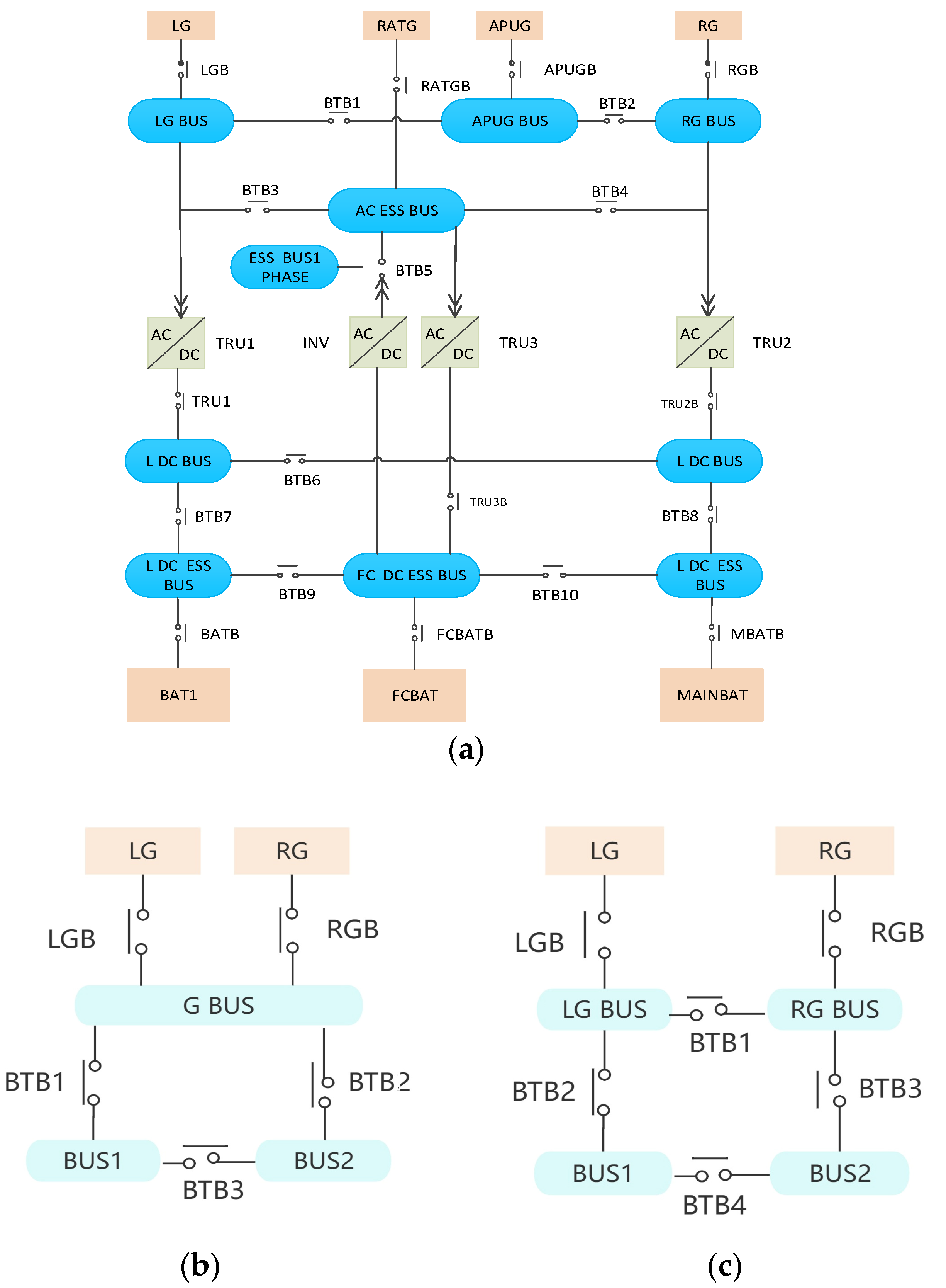
2.1. Typical Structure and Function Logic of the APS

The aviation power system encompasses essential functions such as power generation, storage, transmission, and supporting load operation.
Figure 1a portrays the typical structure of an APS, while additional aviation power system configurations can be found in reference [40]. The key components and their functionalities in the APS of Figure 1 are outlined below:
Generators (LG and RG): The left and right generators, LG and RG, serve as the primary sources of alternating current (AC) power in the system. They operate independently and provide mutual backup in case of failure.
Auxiliary Power Unit (APU): The APU acts as an auxiliary power source, activating when the main generators LG and RG fail to supply power. It ensures that critical onboard equipment remains operational.
Ram Air Turbine Generator (RATG): The RATG functions as an emergency backup generator, kicking in when both the main generators and the APU fail simultaneously.
Batteries: Multiple batteries are used for power storage. During normal AC power supply operation, they remain in a floating charge state. In the event of a fault, these batteries supply power to the corresponding direct current (DC) load busbars.
Power Transmission Components: Power transmission in the system is facilitated by various components such as contactors, relays, circuit breakers, current transformers, and connection busbars. These components play crucial roles in circuit protection, regulation, and control.
Power Conversion Devices: The system’s DC-to-AC (DC-to-AC) and AC-to-DC (AC-to-DC) power conversion is achieved through inverters (INV) and transformer rectifiers (TRU), respectively.
Load Busbars: Also known as power supply busbars, load points, or sink nodes, these AC and DC load busbars support the operation of various loads on the aircraft.
By understanding the components and their functionalities as depicted in Figure 1, one can gain insight into the complex yet robust structure of an aviation power system.

2.2. Three Basic Types of the APS Structure

Based on the classical topology structure of an APS shown in Figure 1a, the power transmission forms of aircraft power grids can be classified into three basic types: open-loop, closed-loop, and hybrid, see Figure 1b,c. These configuration types bear some similarities to the radial, looped, and interconnected types in ground power system networks.
(1)
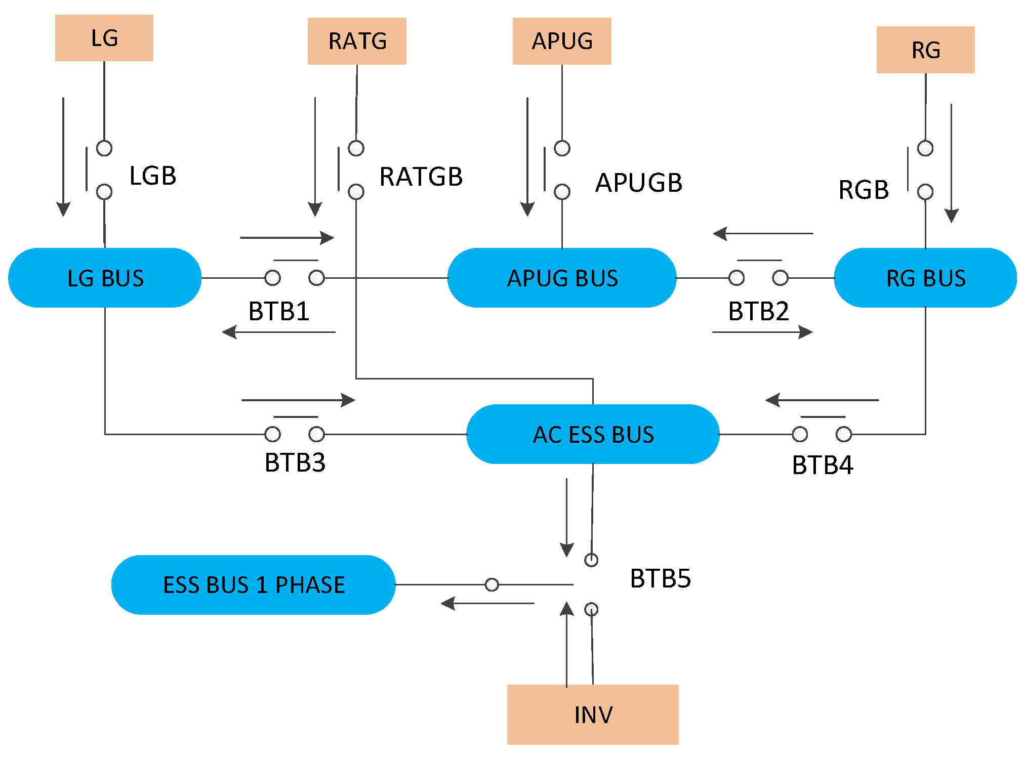
Open-loop Configuration (Similar to Radial Configuration): As shown in Figure 1b (excluding contactor BTB3), the power in an open-loop grid is transmitted to power busbars or electrical equipment through a single channel. This configuration is structurally simple but has relatively low reliability as the power supply to electrical equipment will be lost in the case of a fault in the supply channel.
(2)
Closed-loop Configuration (Similar to Looped Configuration): As depicted in Figure 1b (including contactor BTB3), a closed-loop grid connects load busbars BUS1 and BUS2 through the closed BTB3, forming a “box”-shaped closed-loop structure. This configuration allows load busbars or loads to obtain power from multiple channels, achieving redundant power supply and significantly improving power supply reliability. Closed-loop grids are commonly used in parallel power supply systems.
(3)
Hybrid Configuration (Similar to Interconnected Configuration): As illustrated in Figure 1c, a hybrid grid combines the characteristics of open-loop and closed-loop grids. Under normal conditions, BTB1 and BTB4 are open. When a generator or contactor fails, causing power loss to a certain busbar, the corresponding contactor will close, enabling a dual-redundancy fault-tolerant power supply through a grid reconfiguration. This configuration further enhances the reliability and fault tolerance of the power supply system through flexible grid structure changes.

2.3. Redundancy and Fault-Tolerant Power Supply Requirements

In an APS, components such as generators, inverters, and connectors are relatively common sources of failure. As the primary power supply equipment, a generator’s failure can lead to the entire power system failing. Inverters are responsible for converting DC power to AC power, which is crucial for supplying power to critical flight loads. Therefore, their failure can also significantly impact system reliability. Connectors handle the electrical connections between components, and due to factors like vibration and temperature changes, they may become loose or damaged, affecting the normal operation of the system.
The failure of these devices and components can be caused by various factors, including but not limited to design flaws, manufacturing quality issues, harsh operating environments, and improper maintenance. To reduce the occurrence of failures, aviation power systems often employ redundant design and fault-tolerant technology to ensure that the system can maintain a certain level of power supply capability even in the event of a single component failure.
In an APS, redundancy and fault-tolerant power supply are crucial measures to ensure power supply reliability. Redundancy in a power supply requires the power supply system to provide power to loads from multiple channels, while a fault-tolerant power supply demands that the system maintain the power supply to loads even under multiple failures. For flight-critical loads, which have the highest reliability requirements for power supply missions, a power supply system with more than four redundancies is typically required to meet fault-tolerant power supply demands.

3. Construction Method of APS-RPNM

3.1. Five Types of Structure of the Components of an APS

Five structures can be defined for components of an APS, see Figure 2a–e.
Specifically, based on Figure 1, to ensure a redundant power supply for each load busbar in an aviation power system, each component may possess m input components (m ≥ 0, referring to the components that directly supply current to component C) and n output components (n ≥ 0, referring to the direct recipients of current from component C). Depending on the ratio of m to n, the system structure categorizes component C into five scenarios:
(1)
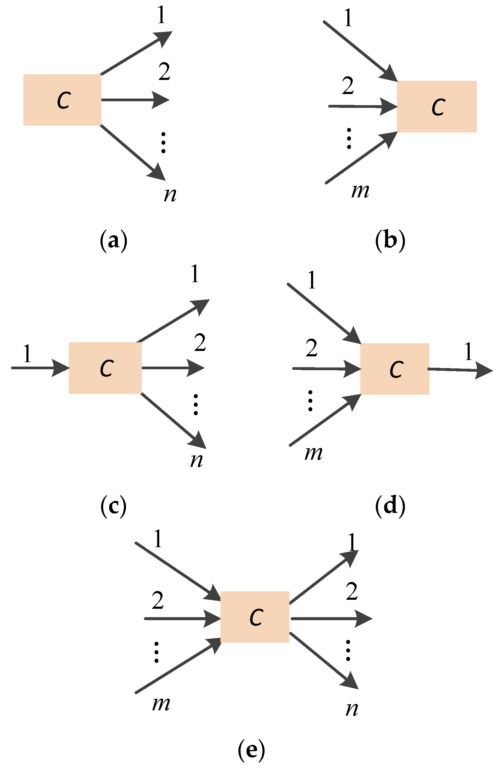
None-Input-to-Multiple-Output (NIMO) structure, where m = 0 and n ≥ 1, indicating that component C receives no direct input but supplies current to multiple outputs.
(2)
Multiple-Input-to-None-Output (MINO) structure, where m ≥ 1 and n = 0, implying that component C receives current from multiple sources but does not directly output it to any component.
(3)
Single-Input-to-Multiple-Output (SIMO) structure, with m = 1 and n ≥ 1, signifying that component C has a single input source and distributes current to multiple outputs.
(4)
Multiple-Input-to-Single-Output (MISO) structure, where m ≥ 2 and n = 1, meaning component C receives current from multiple sources but directs it to a single output.
(5)
Multiple-Input-to-Multiple-Output (MIMO) structure, characterized by m ≥ 2 and n ≥ 2, indicating that component C both receives current from and supplies current to multiple components simultaneously.

3.2. Mapping Rules for Components to the Nodes of APS-RPNM

Under the assumption of fault independence, this paper analyzes the functional/fault logic relationship between component C and its input and output components across five different structures. It further proposes a method for mapping component C to the corresponding nodes in the APS-RPNM, which is detailed as follows:
(1)
In the NIMO structure, if component C functions normally, it does not affect the working state of its output components. However, if component C fails, all of its output components will fail to operate properly.
Based on this logical relationship, component C exhibits two states: normal operation and fault, represented by 0 and 1, respectively. Typically, the failure rate of each component in the power system remains constant at λ. Therefore, the probability of component C being in a failure state is 1 − eλt, while the probability of it being in a normal state is eλt. Consequently, a unique two-state node C is established for component C, and the conditional probability distribution of the node C is determined accordingly:
Pr ( C = 0 ) = e λ t Pr ( C = 1 ) = 1.0 e λ t
(2)
In the MINO structure, due to the independence of component failures, if component C is in a fault state, it cannot function regardless of whether its input components are capable of providing normal current to C. Conversely, when C is in a non-fault state, it operates normally if any of its input components are capable of supplying current; otherwise, if none of the input components can provide current to C, it remains inoperable even though component C is not faulty.
Based on this logical relationship, component C is characterized by three states: normal operation, fault state, and a state where it is non-faulty yet unable to operate normally. For component C in the MINO structure, a node containing these three states is established, represented by 0/1/2 respectively. Additionally, a conditional probability distribution equivalent to this logic is formulated for the node C.
Pr ( C = 0 | X , X π ( C ) X = 0 ) = e λ t Pr ( C = 1 | X , X π ( C ) ) = 1.0 e λ t Pr ( C = 2 | X , X π ( C ) X = 0 ) = 0.0 Pr ( C = 0 | X , X π ( C ) X 0 ) = 0.0 Pr ( C = 2 | X , X π ( C ) X 0 ) = e λ t
where π (C) is the parent set of node C.
(3)
In the MISO and SIMO structures, although the number of inputs and outputs of component C differs from that in the MINO scenario, the functional/fault logic remains identical (where, when C is in state 1 or 2, it cannot provide input current to its output components). Therefore, for component C in these two structures, the same three-state node and conditional probability distribution as in case (2) are constructed.
Based on the analysis from (1) to (3), if component C belongs to any of the first four structural patterns, the node in APS-RPNM constructed for component C corresponds uniquely to it. The equivalent APS-RPNM structure of node C is identical to those depicted in Figure 2a–d.
(4)
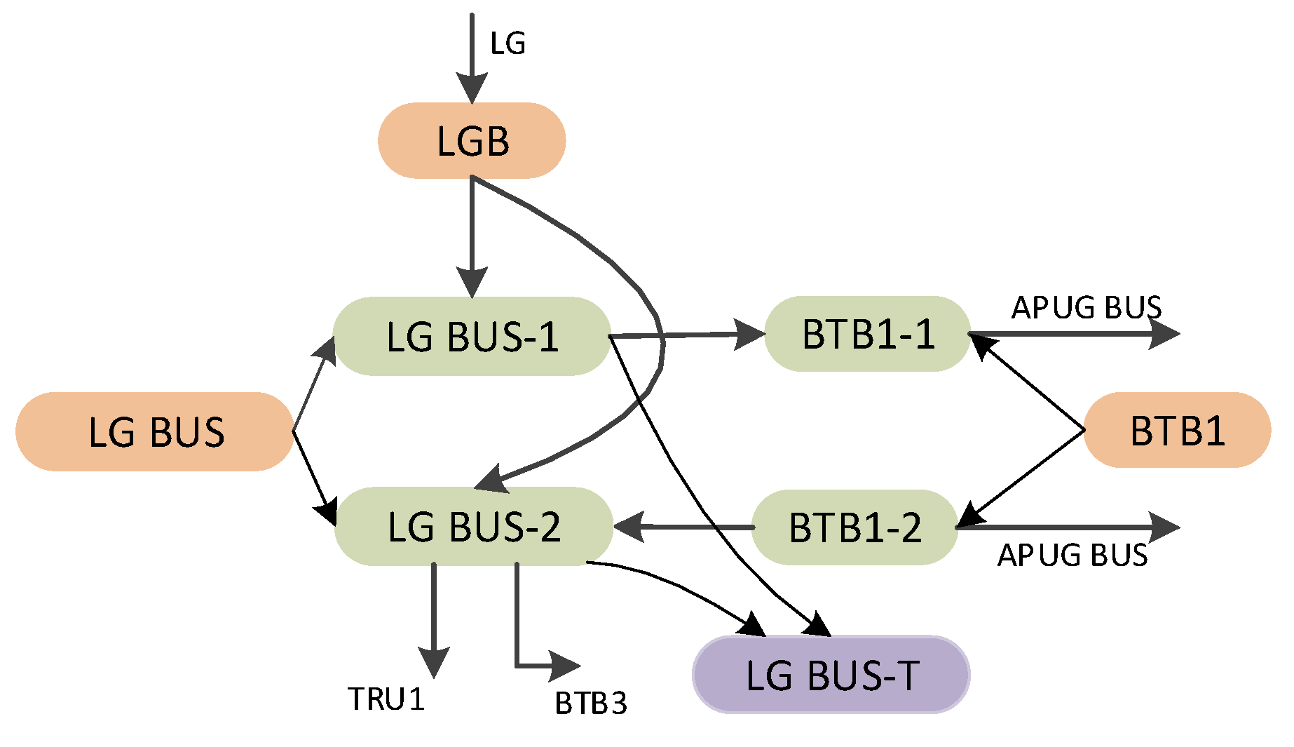
In the MIMO structure, for component C, the input components powering its i-th output component may be different from those powering its j-th output component. For example, considering the LGBUS component in Figure 1, it exhibits a 3:2 structure or configuration, with three outputs and two input components. Specifically, both BTB3 and TRU1 are powered by the same input components, namely LGB and BTB1, whereas BTB1 is solely powered by LGB (refer to Figure 3).
If the input components powering the i-th and j-th output components differ, then, in the APS-RPNM, the grandparent nodes of output components i and j must necessarily be different. Constructing only a single corresponding node for component C would fail to accurately represent the distinct grandparent nodes of the i-th and j-th output components. To address these issues, this paper introduces the concepts of pathway patterns and sub-nodes.
Pathway Definition: For component C, if the input components providing current to the output component i are denoted as i1, i2,…, imi, then component i and the set {i1, i2imi} constitute a pathway pattern (simply referred to as a pathway) of component C. Here, i and {i1, i2imi} are respectively called the output and input components of that pathway pattern. Furthermore, for another pathway formed by component j (where ji) and the set {j1, j2jmj}, if the sets {i1, i2imi} and {j1, j2jmj} are identical, the two pathways are considered the same.
In an m:n scenario (i.e., a MIMO structure), component C has s distinct pathways, where 1 ≤ sn. Based on the pathway definition, the discussion is categorized as follows:
  • When s = 1, all pathways are the same, and the grandparent nodes of each output component are identical. Therefore, constructing a three-state node C can accurately represent the function/failure logic between component C and its input/output components.
  • When 2 ≤ sn, there exist different pathways for component C. The grandparent nodes of output components on different pathways are necessarily distinct. Hence, the key to constructing the corresponding node for component C in this case lies in accurately describing these s different pathways.
For scenario (ii), this paper proposes to construct s two-state (0/1) sub-nodes, denoted as C-1, C-2…C-s. The child and parent nodes of sub-node C-k represent the output and input components on pathway k, respectively. In addition, a common parent node C, also in a two-state (0/1) format of these sub-nodes, needs to be established to represent the failure parameters of component C. The conditional probability distribution of node C follows Equation (1). Additionally, the logical relationship between node C and sub-node C-k is as follows: ① When component C fails, the pathway k represented by C-k becomes blocked and cannot supply power to the output component on that pathway; ② When component C is functional and at least one of the input components on pathway k is operational, the pathway represented by C-k can provide power to the output component on that pathway. To fully articulate this logic, the conditional probability distribution of sub-node C-k is set as described below.
The logical relationship between node C and sub-node C-k is defined as:
  • When component C fails, the pathway represented by C-k becomes non-functional, unable to transmit power to the output component on that pathway.
  • If component C is operational and at least one input component on pathway k is working, the pathway represented by C-k can transmit power to its output component.
To encapsulate this logic, the conditional probability distribution of sub-node C-k is determined as outlined below.
Pr ( C k = 1 | X , X π ( C k ) C = 1 ) = 1.0 Pr ( C k = 0 | X , X π ( C k ) C = 1 ) = 0.0 Pr ( C k = 0 | X , X π ( C k ) X = 0 C = 0 ) = 1.0 Pr ( C k = 1 | X , X π ( C k ) X = 0 C = 0 ) = 0.0 Pr ( C k = 0 | X , X π ( C k ) X 0 C = 0 ) = 0.0 Pr ( C k = 1 | X , X π ( C k ) X 0 C = 0 ) = 1.0
In Equation (3), π ( C k ) represents the other parent nodes of node C-k besides node C.
Taking the LG BUS component in Figure 1 as an example, and combining it with Figure 3, it can be clearly seen that the LG BUS exhibits two distinct pathway modes. The nodes constructed in ASP-RPNM for the LG BUS are shown in Figure 4. Specifically, in Pathway 1, the input is undertaken by the LGB component and its output is connected to the BTB1 component, while in Pathway 2, apart from LGB, BTB1 also serves as an input component and the output is distributed to the TRU1 and BTB3 components. Based on the proposed construction theory, this paper constructs sub-nodes LG BUS-1 and LG BUS-2 for these two pathway modes respectively, and clearly shows these sub-nodes and their common parent node LG BUS.

3.3. Construction of an Equivalent APS-RPNM

When constructing an equivalent APS-RPNM for the power system, the nodes corresponding to each component were initially established according to the method outlined in Section 3.1. Subsequently, to enhance the precision of the network model, a methodology is introduced to clarify the relationship between each node’s parent nodes and establish corresponding target nodes, thereby safeguarding the integrity and accuracy of the entire model.
The determination of the parent nodes of node C or C-k follows these principles: For the input component X of node C or C-k, if component X has only one corresponding node X’, then node X’ is the parent node of node C or C-k. If component X has multiple corresponding sub-nodes, such as X-1, X-2, etc., then among these sub-nodes, the node whose output component is C is the parent node of node C. Taking Figure 4 as an example, the process of determining the parent nodes of the node LG BUS-2 is as follows: The input components of node LG BUS-2 are LGB and BTB1. Among them, the component LGB has a unique corresponding node LGB, so node LGB is a parent node of LG BUS-2; while the component BTB1 has two corresponding sub-nodes, BTB1-1 and BTB1-2 (see Figure 5). Since the output component of sub-node BTB1-2 is LG BUS, BTB1-2 is another parent node of LG BUS-2.
The core task of the power system is to ensure the normal operation of loads on different load busbars. To this end, this paper constructs a two-state leaf node describing the load operating state as the target node, where states 0 and 1 represent the busbar’s inability and ability to support load operation, respectively.
For instance, based on the above method of clarifying parent nodes and constructing target nodes, this paper constructs an equivalent APS-RPNM for the three components of LG BUS, BTB1, and LG in Figure 1, as shown in Figure 6.
If the load busbar has only one corresponding node in APS-RPNM, that node directly serves as the parent node of the target node, and the conditional probability distribution is set according to Equation (4). This reflects the physical situation where the busbar cannot support the load when it malfunctions or there is no current passing through it.
If the busbar corresponds to multiple sub-nodes in APS-RPNM, these sub-nodes will collectively serve as the parent nodes of the target node, and the conditional probability distribution will be set according to Equation (5). This probability distribution indicates that when all pathways lose power, the busbar will be unable to support the load operation.
In Equations (4) and (5), Y-T denotes the target node representing the load operating state on busbar Y. The physical meaning of these equations is that when the busbar malfunctions or there is no current, or when all pathways lose power, the busbar cannot support the load operation; otherwise, it can.
Pr ( Y T = 0 | Y = 0 ) = 1.0 Pr ( Y T = 1 | Y = 1 Y = 2 ) = 1.0
Pr ( Y T = 0 | Y k , Y k = 0 ) = 1.0 Pr ( Y T = 1 | Y k , Y k = 1 ) = 1.0

4. Case Study

In this section, the AC subsystem of the typical power system depicted in Figure 1 is taken as the subject of study. Utilizing the proposed modeling methodology, an equivalent APS-RPNM is constructed for this subsystem. Leveraging the APS-RPNM calculation software GeNIe 2.0, this paper conducts a power supply reliability analysis on the network. To demonstrate the superiority of the presented approach in terms of calculation and expression, a comparative discussion is also included, contrasting the analysis results with those obtained through the classic minimal path set-based reliability analysis method.

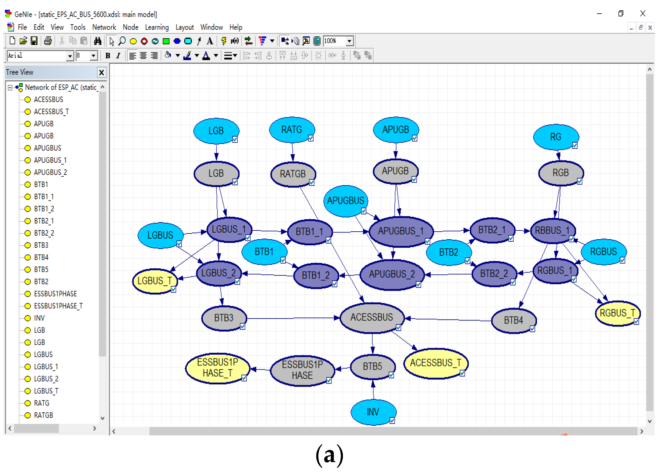
4.1. Construct the Equivalent APS-RPNM

The input-output relationship serves as the fundamental basis for model construction in this paper, primarily determined by the system’s redundant structure. According to the redundancy design scheme illustrated in Figure 1 for the AC subsystem, the power supply strategy is as follows:
The AC load busbars LG BUS and RG BUS are designed with triple redundancy, AC ESS BUS with quadruple redundancy, and ESS BUS 1 PHASE achieves quintuple redundancy. Under normal operating conditions, the left and right power supplies (LG and RG) form two separate power supply channels, providing electricity to all of the AC busbars in the entire system. In the event of a failure in LG or RG, APUG will automatically activate, replacing the failed power supply. If two generators among LG, RG, and APUG cease to function, the remaining generator will undertake the task of powering all AC busbars. In extreme cases where LG, RG, and APUG all fail, RATG will intervene to supply power to AC ESS BUS and ESS BUS 1 PHASE. When LG, RG, APUG, and RATG all fail, ESS BUS 1 PHASE will obtain electricity from the DC power supply system through INV.
Based on the aforementioned redundancy design scheme, this paper has crafted Figure 7, which clearly illustrates the input-output relationships of the AC subsystem depicted in Figure 1.
Utilizing the modeling theory presented in this paper, the construction of the equivalent APS-RPNM for the AC subsystem follows these steps:

4.1.1. Constructing Nodes Based on Component Structures

For components with the NIMO structure, such as LG, we create a corresponding two-state node. Similarly, we create two-state nodes for RATG, APUG, RG, and INV.
For components exhibiting a 1:1 structure, such as LGB, which falls under the SIMO category, a distinct three-state node is established. Analogously, we set up three-state nodes for RATGB, APUGB, RGB, BTB3, BTB4, and BTB5.
For components with 3:1 and 2:1 structures (these two structures belong to the structure of MISO), such as AC ESS BUS and BTB5, establish a three-state node for each.
For the 1:0 structure (which is part of the structure of MINO) of component ESS BUS 1 PHASE, a three-state node is constructed.
For the 2:2 structure (which is part of the structure of MIMO) component APUG BUS, create sub-nodes APUG BUS-1 and APUG BUS-2 to represent its two pathways, and establish a parent node APUG BUS. Apply the same logic to LGU BUS, BTB1, BTB2, and RG BUS.

4.1.2. Determining Parent Nodes

For three-state nodes like LGB, whose input component is LG, because the component LG only has one node in APS-RPNM, which corresponds to itself, the parent node of LGB in the network is the node LG. This logic applies to all other three-state nodes.
The input component of the sub-node APUG BUS-1 is BTB1, while the output component of the sub-node BTB1-1 is APUG BUS. Therefore, according to the proposed construction method, the parent node of APUG BUS-1 is BTB1-1. Similarly, the parent nodes of other sub-nodes can be determined. Nodes such as LG, RATG, APUG, RG, INV, LG BUS, BTB1, APUG BUS, BTB2, and RG BUS in APS-RPNM are considered root nodes and do not require a parent node determination.

4.1.3. Identifying the Target Nodes

The AC system supports load operation through busbars LG BUS, RG BUS, AC ESS BUS, and ESS BUS 1 PHASE. Therefore, corresponding target nodes LG BUS-T, RG BUS-T, AC ESS BUS-T, and ESS BUS 1 PHASE-T are established for the network model.
The equivalent APS-RPNM formed through steps (1) to (3) is shown in Figure 8.

4.1.4. Determining Conditional Probability Distributions for Nodes

In the developed APS-RPNM, nodes are categorized into four distinct types: root nodes, three-state nodes, sub-nodes, and target nodes. Utilizing the component failure rates tabulated in Table 1, the conditional probability distributions for root nodes and three-state nodes are derived through Equations (1) and (2), respectively. To illustrate, Table 2, Table 3, Table 4 and Table 5 present the conditional probability distributions for various node types within the APS-RPNM. The failure rates in Table 1 also can be found in References [11,19].
Specifically, considering a system operational duration of t = 100 h, the conditional probability distributions for the root node LG and the three-state node LGB, derived from the aforementioned equations, are outlined in Table 2 and Table 3, respectively.
For sub-nodes, their conditional probability distributions are ascertained using Equation (3). As an example, Table 4 showcases the conditional probability distribution for the sub-node LG BUS-1.
As for target nodes, whether they possess single or multiple parent nodes, their conditional probability distributions are computed using Equations (4) or (5), respectively. To demonstrate, Table 5 exhibits the conditional probability distribution for the target node AC ESS BUS-T.
By following these procedures, this paper has effectively established an equivalent APS-RPNM which is optimally suited for conducting comprehensive system reliability analyses.

4.2. System Reliability Calculation and Analysis

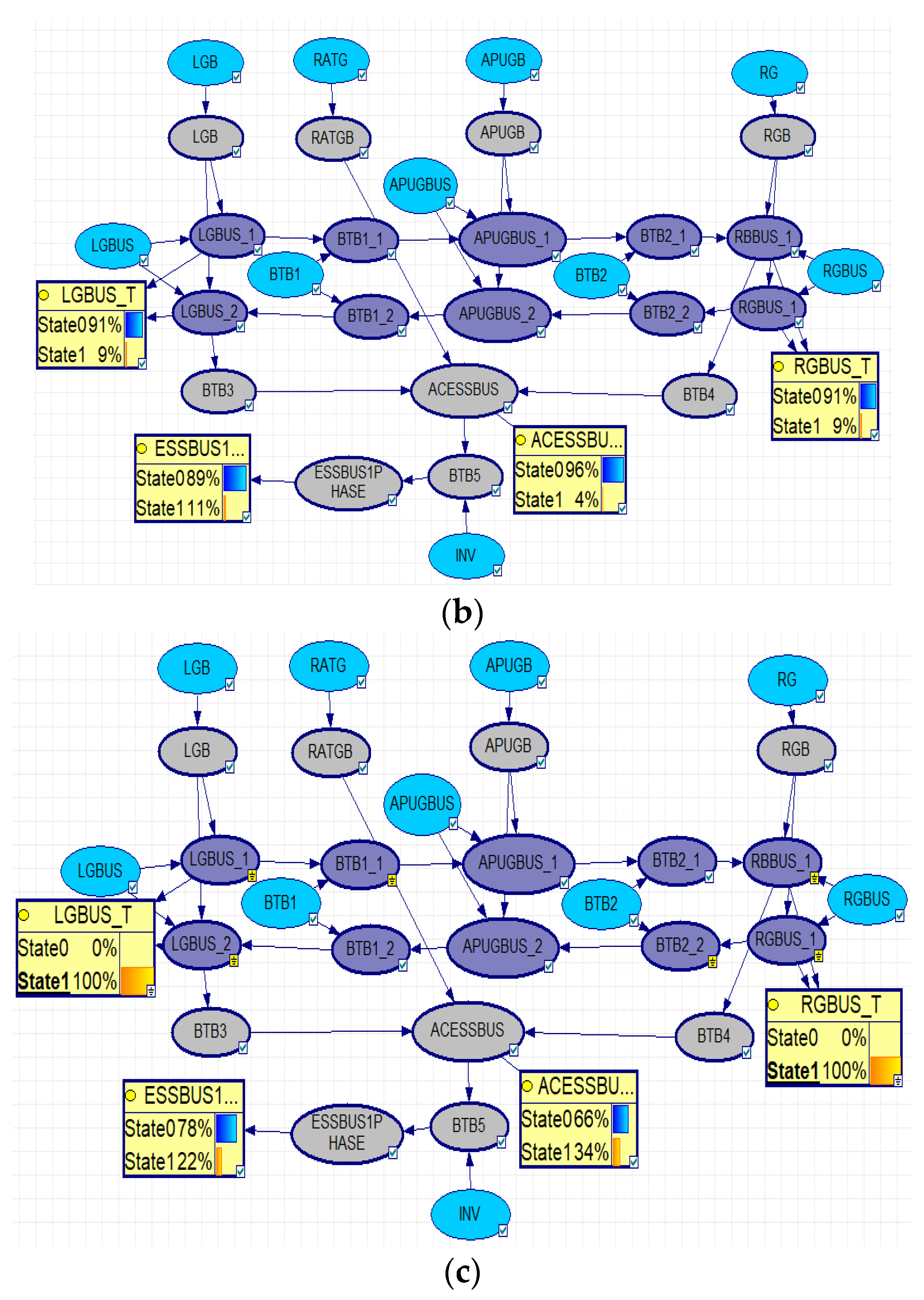
4.2.1. Reliability Analysis Results Based on APS-RPNM

Calculation of Power Supply Reliability

By establishing an APS-RPNM, this paper determines the marginal probability values of each target node being in state 0. Values such as Pr(LG BUS-T = 0), Pr(RG BUS-T = 0), Pr(AC ESS BUS-T = 0), and Pr(ESS BUS 1 PHASE-T = 0) directly reflect the power supply reliability of the load busbars they represent. To quantify this reliability, the paper employed GeNIe 2.0 software to conduct detailed calculations of the network model’s reliability at different time points. Figure 9a,b illustrate the APS-RPNM constructed using this software and the reliability calculation results, respectively. Additionally, Table 6 lists the reliability data at various time points, such as t = 800 h, 1600 h, up to 8000 h, in its second to fourth columns, while the associated computation times are provided in Table 7.

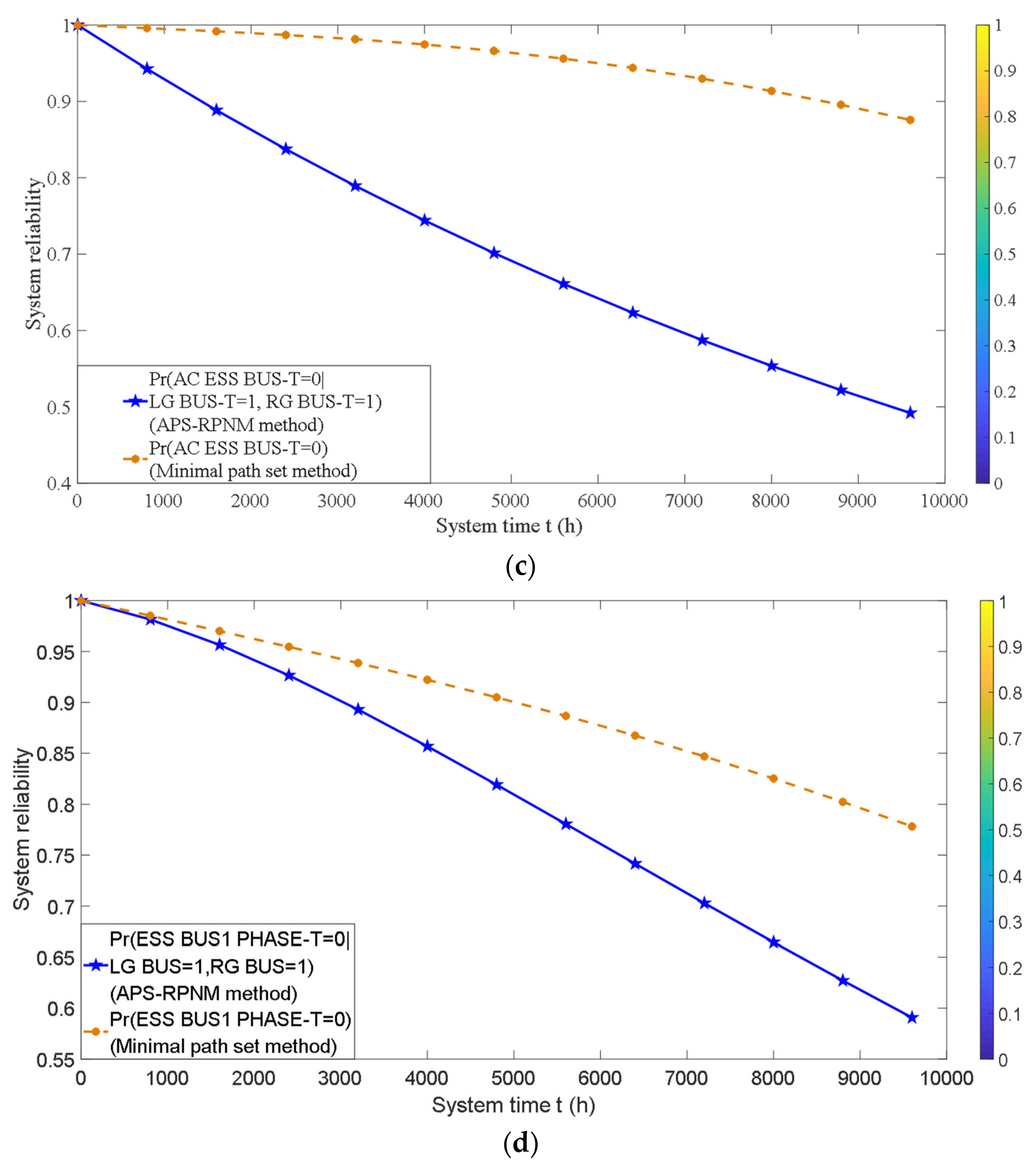
Analysis of Power Supply Dependency

Compared to traditional reliability analysis methods (e.g., reliability block diagrams, minimal cut sets), our probability network has demonstrated its unique advantages in system dependency analysis. These advantages have been widely proven [41]. Therefore, the APS-RPNM constructed in this paper possesses the same capability for system dependency analysis.
In the context of aircraft power systems, loads are distributed throughout the entire aircraft. To comprehensively understand the operational status of the power supply system, this paper focuses not only on the reliability of individual power supply busbars but also on their probabilities of occurrence in different combination states. This involves examining the interactions between various power supply paths and the resulting dependencies between the power supply states of different load busbars. For instance, it explores the reliability of some or all load busbars operating simultaneously, or the probability of other (emergency) load busbars functioning normally when a particular (non-essential) power supply busbar fails.
These questions can be answered using the model presented in this paper. Specifically, multiple target nodes are set at a specific time ‘t’ with states (0 or 1) as evidence variables in the model. Then, these variables are used to derive marginal and posterior probability results through reasoning. These outcomes reflect the power supply probabilities of multiple busbars supporting loads under given state combinations or conditions.
For example, at t = 5600 h, if nodes LG BUS-T = 0 and RG BUS-T = 0 are set, and the marginal probability Pr(LG BUS-T = 0, RG BUS-T = 0|t = 5600) is calculated to be 0.855211, this probability value indicates the reliability of both the left and right main load points, LG BUS and RG BUS, being able to supply power normally at t = 5600 h. Similarly, if nodes LG BUS-T = 1 and RG BUS-T = 1 are set as evidence variables, the posterior probability Pr(AC ESS BUS-T = 0|LG BUS-T = 1, RG BUS-T = 1, t = 5600 h) can be calculated as 0.661106 (see Figure 9c). This value represents the reliability of the emergency busbar AC ESS BUS to support emergency onboard AC equipment when both the left and right main load points cannot supply power to the onboard AC equipment. This data provides valuable reference information for the design of emergency power supply subsystems.
By setting evidence variables in a similar manner, this paper calculates power supply probabilities under various combination states or conditions, thereby providing a valuable theoretical reference for system reliability design. Due to space limitations, this paper only showcases the power supply probability calculation results for four relevant scenarios in Figure 10, based on the model constructed using GeNIe 2.0 software (see Figure 9).
In Figure 10, Scenario 1 means the probability that both LG BUS and RG BUS can supply power normally at the same time; Scenario 2 means the probability that all four busbars can supply power normally at the same time; Scenario 3 means the reliability of power supply for the emergency busbar AC ESS BUS after both LG BUS and RG BUS fail; Scenario 4 means the reliability of power supply for the emergency busbar ESS BUS 1 PHASE under the condition that both LG BUS and RG BUS fail.

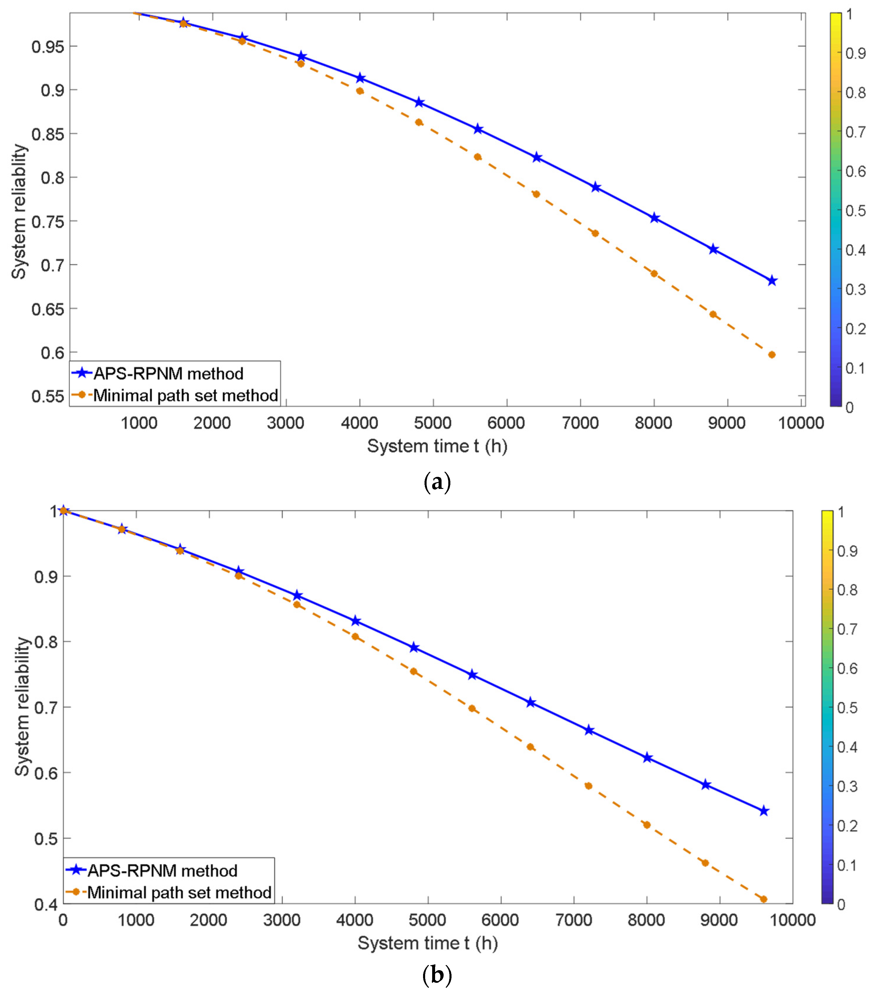
4.2.2. Reliability Analysis Results Based on Minimal Path Sets

To validate the effectiveness of the modeling approach proposed in this study, the paper adopts the minimal path set (MPS) technique to conduct an in-depth reliability analysis of the system. Specifically for the busbar LG BUS, there are three minimal path sets as follows:
A 1 = ( 1 ,   2 ,   3 ) A 2 = ( 7 ,   6 ,   5 ,   4 ,   3 ) A 3 = ( 11 ,   10 ,   9 ,   8 ,   5 ,   4 ,   3 )
For ease of description, the components in the system, namely LG, LGB, LG BUS, BTB1, APUG BUS, APUGB, APUG, BTB2, RG BUS, RGB, and RG, are sequentially numbered from 1 to 11.
Utilizing the system reliability calculation Formula (6) based on the MPS, this paper derives the power supply reliability Formula (7) for LGBUS:
R = P ( i = 1 m A i ) = i = 1 m P ( A i ) i < j m P ( A i A j ) + i < j < k = 3 m P ( A i A j A k ) + + ( 1 ) m 1 P ( i = 1 m A i )
RLGBUS = P(A1A2A3) = P(A1) + P(A2) + P(A3) − P(A1A2) − P(A1A3) − P(A2A3) + P(A1A2A3)
In the formula, P(A1) = R1 R2 R3, P(A2) = R3 R4 R5 R6 R7, P(A3) = R3 R4 R5 R8 R9 R10 R11, P(A1A2) = R1 R2 R3 R4 R5 R6 R7, P(A1A3) = R1 R2 R3 R4 R5 R8 R9 R10 R11, P(A2A3) = R3 R4 R5 R6 R7 R8 R9 R10 R11, P(A1A2A3) = R1 R2 R3 R4 R5 R6 R7 R8 R9 R10 R11, R i = e λ i t , where Ri represents the reliability of component i.
At a specific system time point, such as t = 800 h, by substituting the failure rate data of each component into Formula (7), the power supply reliability of LG BUS after 800 h of operation is calculated as RL GBUS = 0.995041. This result aligns with the outcome obtained from APS-RPNM. Similarly, Formula (6) is also used to calculate the power supply reliability of other busbars such as RGBUS and APUGBUS, and the results are compared with those from the probability model. For details, refer to columns 5 to 7 in Table 6, where the data are identical to the data obtained from APS-RPNM.

4.3. Analysis of the Power Supply Reliability Results

Formula (6) is the precise solution formula for the minimal path set method. Comparing the data in Table 6, it can be seen that the calculation results based on the probability network are the same as those from Formula (6), verifying the correctness of the method proposed in this paper. Next, the characteristics of this modeling method will be analyzed from two aspects: modeling and calculation.

4.3.1. Model Structure Analysis

Comparing Figure 1, Figure 3 and Figure 8, it can be seen that the APS-RPNM established in this paper is highly consistent with the system structural schematic diagram. The main difference lies in the fact that the APS-RPNM visualizes the hidden functions/failure logic and probability data in the schematic diagram, making the APS-RPNM computable compared to the schematic diagram. This modeling approach, which is consistent with the structural schematic diagram, has the following advantages.
The ease of model manipulation is closely related to the representation method of the model. Representation methods that are close to the physical structure or schematic diagram of the system usually have better manipulability. In addition, in the traditional reliability modeling process, different engineers often model from different perspectives based on their own experience, making it difficult to avoid modeling errors or even mistakes introduced by human cognition. However, the modeling method proposed in this paper is consistent with the system’s structural schematic diagram, ensuring that different modelers obtain the same model according to this method, thereby guaranteeing the correctness of the model.

4.3.2. Analysis of Computational Efficiency

The modeling method proposed in this paper has significant advantages in computational efficiency, mainly reflected in its ability to simultaneously calculate the power supply reliability of all load busbars.
Firstly, as shown in Figure 8 and Figure 9, compared to traditional methods that can only calculate the power supply reliability of one load busbar at a time, the method proposed in this paper can process the calculation of all load busbars in the same model at once. This feature is particularly important in the context of the rapid development of more/all-electric aircraft and the increasing number of aviation power system load busbars. For a system with n busbars, traditional methods require n separate calculations, while the method in this paper can be completed through a one-time calculation, greatly improving the computational efficiency of system power supply reliability.
Secondly, the advantage of the method proposed in this paper in terms of computational efficiency can be further verified through actual data comparisons. According to the data in Table 7, when calculating the power supply reliability of four AC busbars in the system at eight different times, the method in this paper takes less than 8 ms, while the traditional minimal path set method takes about 328 ms. This significant difference fully demonstrates the noticeable improvement in computation speed of the method proposed in this paper.
Finally, analyzing the computational complexity of the two methods from a theoretical perspective can further explain the high computational efficiency of the method set forth in this paper. The complexity of the traditional minimal path set method mainly depends on the number of minimal path sets, while the complexity of the probabilistic network method proposed in this paper mainly depends on the maximum number of parent nodes in the model. Through topological analysis, it can be seen that for the components in the minimal path set of the power supply busbar Y, if a component A has the largest number of input components (denoted as a), then the busbar Y has at least a minimal path sets. Since the topological structure of the model proposed in this paper is consistent with the functional schematic diagram, the maximum number of parent nodes of node A is a, which means that the maximum number of parent nodes in the probabilistic network built in this paper cannot be greater than the number of minimal path sets. The reasonableness of this analysis can be verified by analyzing the number of minimal path sets and the maximum number of parent nodes for the power supply busbars LG BUS, RG BUS, AC ESS BUS, and ESS BUS 1 PHASE. The number of minimal path sets for these four busbars is 3, 3, 7, and 8, respectively, and the maximum number of parent nodes is 2, 2, 3, and 3. In addition, for multiple power supply busbars in large and complex power supply networks, the method in this paper can describe them all in the same model, making the computational complexity of reliability independent of the number of busbars. In contrast, traditional methods require calculating the power supply reliability of each busbar individually, so the calculation time increases with the number of busbars.
In summary, theoretically speaking, the computational complexity of the method in this paper is lower than that of the traditional minimal path set method.

4.3.3. Analysis of Power Supply Dependence between Different Load Points

Compared to traditional methods, the approach proposed in this paper not only boasts high computational efficiency but also accurately considers the dependence effects of power supply paths between different busbars, enabling a more precise analysis of the overall system reliability. The analysis is as follows:
In the probabilistic network model, when the system has been operating for 5600 h, the reliability of both LG BUS and RG BUS supplying power normally simultaneously is 0.855211. However, using traditional methods, since they can only obtain the minimal path sets for each power supply busbar, the reliability of LG BUS and RG BUS supplying power normally is calculated by multiplying their respective reliabilities, resulting in a value of 0.907319 × 0.907319 = 0.823228748.
The probability value obtained by the method in this paper is significantly higher than that of the traditional method. This is mainly because the traditional method does not fully consider the influence of shared components in the system on the power supply status of multiple load points during the calculation process. For example, the component APUG appears in the minimal path sets of both LG BUS and RG BUS. The traditional multiplication calculation method is equivalent to treating the APUG component on the minimal path set of LG BUS and the APUG component on the minimal path set of RG BUS as independent and different components. This means that the failure impact of APUG is doubly considered during the calculation process, leading to a calculated reliability that is lower than the true value. Moreover, this error accumulates over time, increasing the discrepancy. This explains why the reliability curve obtained by the traditional method in Figure 10a is lower than that of the method proposed in this paper. Similarly, the results in Figure 10b can also be explained by this reasoning.
Additionally, after the main load points LG BUS and RG BUS fail to supply power, the theoretical power supply reliability of the emergency busbar AC ESS BUS should be measured using the conditional probability Pr(AC ESS BUS-T = 0|LG BUS-T = 1, RG BUS-T = 1). However, in the calculation of the minimal path set method, based on the principles of conditional probability calculation, this value is approximately equal to Pr(AC ESS BUS-T = 0) × Pr(RG BUS-T = 1) × Pr(RG BUS-T = 1)/[Pr(RG BUS-T = 1) × Pr(RG BUS-T = 1)] = Pr(AC ESS BUS-T = 0). This actually only represents the reliability of AC ESS BUS in an independent power supply state and fails to consider the adverse effects of the power supply status of LG BUS and RG BUS on its reliability.
Upon deeper exploration, it can be observed that when the main load points lose power, it implies that LG BUS and RG BUS have failed. These two busbars are also critical components in the power supply path of AC ESS BUS. Their failure directly reduces the power supply path of AC ESS BUS, thereby decreasing its power supply reliability. This point can be clearly verified by comparing the results in Figure 7, Figure 8, and Figure 10c. Similarly, the curve changes presented in Figure 10d also follow this logic.
To more accurately assess system reliability, this paper innovatively constructs a new model. This model not only integrates the functions and failure logic of all components in the system but also introduces sub-nodes in different power supply paths to represent shared components. These sub-nodes are connected by a common parent node, precisely depicting the dependence between different power supply paths. This model design provides analysts with a powerful tool for comprehensive and accurate analysis of power system reliability under various power supply combination states and conditions, laying a solid theoretical foundation for ensuring the stable operation of the power system.

4.3.4. Main Contributions of This Proposed APS-RPNM

This paper proposes the APS-RPNM for reliability analysis of aviation power systems. Based on the analysis in (1)–(3), the proposed method has achieved significant results in terms of accuracy, computational efficiency, and system dependency analysis capabilities. The specific contributions are summarized as follows:
(i)
Significant improvement in model accuracy and consistency: By constructing a probabilistic network model that closely corresponds to the system structure schematic, this paper successfully visualizes the functional/fault logic and probability data originally hidden in the schematic. This modeling approach not only greatly improves the accuracy of the model but also ensures its consistency with the actual operation of the system, laying a solid foundation for subsequent reliability analysis.
(ii)
Innovation in computational efficiency: Compared to traditional methods that require calculating the power supply reliability of each load busbar individually, the method proposed in this paper achieves a significant improvement in computational efficiency by processing all busbar calculations in parallel within the same model. Especially when dealing with large and complex power supply networks containing many busbars, the advantages of this method become more apparent, providing strong support for rapid decision-making in practical applications.
(iii)
Comprehensive strengthening of system dependency analysis capabilities: Traditional methods often have shortcomings in dealing with dependency between power supply paths, while the method proposed in this paper successfully solves this problem by integrating the functional/fault logic of all components into the same model. This not only makes the analysis of the overall system reliability more accurate but also allows for accurate calculations of the relevant conditional probabilities in complex scenarios such as emergency power supply conditions, providing a more comprehensive theoretical support for the reliability design and optimization of the system.

5. Conclusions

The APS-RPNM proposed in this study offers a groundbreaking approach to reliability analysis of aviation power systems. The key contributions and advantages of this methodology are highlighted below, based on the comprehensive analysis conducted using mathematical models, simulations, and case studies.
Firstly, by constructing a probabilistic network model that closely aligns with the aviation power system architecture, the APS-RPNM achieves a high degree of accuracy and consistency in representing system functions and fault logic. This approach not only ensures a tight correlation between the model and actual system operations but also lays a solid foundation for subsequent reliability assessments. The effectiveness of this modeling strategy is evident from the detailed analysis presented in Figure 2, Figure 3, Figure 4, Figure 5, Figure 6, Figure 7, Figure 8 and Figure 9.
Secondly, the APS-RPNM demonstrates remarkable computational efficiency. By integrating all power supply busbars into a single model, the proposed methodology enables the calculation of power supply reliability for all busbars in a single inference. As demonstrated in our testing, the APS-RPNM calculates the power supply reliability of four AC busbars at eight different time points in less than 8 ms, significantly outperforming the traditional minimal path set method, which takes approximately 328 ms (see Table 7). This substantial improvement in computational speed is particularly valuable for handling large and complex power supply networks, enabling rapid decision-making in practical applications.
Furthermore, the APS-RPNM significantly enhances system dependency analysis capabilities. By introducing the concepts of sub-nodes and common parent nodes, the model effectively captures the dependencies between different power supply paths. This allows for more accurate calculations of power supply reliability under various conditions, especially in emergency scenarios such as the simultaneous failure of LG BUS and RG BUS (see Figure 10). As evidenced by the case studies presented in the paper, the APS-RPNM accurately reflects the impact of common component failures on system reliability, providing comprehensive theoretical support for system reliability design and optimization.
In summary, the APS-RPNM represents a significant advancement in the field of aviation power system reliability analysis. With its precision, efficiency, and comprehensive dependency analysis capabilities, this model holds tremendous potential for ensuring the safe and stable operation of aviation power systems in the future. Looking ahead, the application of the APS-RPNM in more complex scenarios will be further investigated, and the model will undergo continuous optimization and improvement, with the ultimate goal of bolstering the safe and stable operation of aviation power systems.

Author Contributions

Conceptualization, Y.W.; methodology, Y.W.; software, Y.W.; validation, F.W.; formal analysis, F.W.; investigation, Y.Z.; resources, Y.W.; data curation, S.L.; writing—original draft preparation, Y.W.; writing—review and editing, Y.W.; visualization, Y.Z.; supervision, Y.Z.; project administration, S.L.; funding acquisition, Y.W. and Y.Z. All authors have read and agreed to the published version of the manuscript.

Funding

The research was funded by the Aviation Science Fund of China ASFC-202300130T6003.

Data Availability Statement

Data are contained within the article.

Acknowledgments

The authors thankfully acknowledge the support provided by the Aviation Science Fund of China.

Conflicts of Interest

The authors declare no conflicts of interest.

References

  1. Schäfer, A.W.; Barrett, S.R.; Doyme, K.; Dray, L.M.; Gnadt, A.R.; Self, R.; O’Sullivan, A.; Synodinos, A.P.; Torija, A.J. Technological, economic and environmental prospects of all-electric aircraft. Nat. Energy 2019, 4, 160–166. [Google Scholar] [CrossRef]
  2. Borghei, M.; Ghassemi, M. Insulation materials and systems for more-and all-electric aircraft: A review identifying challenges and future research needs. IEEE Trans. Transp. Electrif. 2021, 7, 1930–1953. [Google Scholar] [CrossRef]
  3. Sahoo, S.; Zhao, X.; Kyprianidis, K. A review of concepts, benefits, and challenges for future electrical propulsion-based aircraft. Aerospace 2020, 7, 44. [Google Scholar] [CrossRef]
  4. Schefer, H.; Fauth, L.; Kopp, T.H.; Mallwitz, R.; Friebe, J.; Kurrat, M. Discussion on electric power supply systems for all electric aircraft. IEEE Access 2020, 8, 84188–84216. [Google Scholar] [CrossRef]
  5. Ebersberger, J.; Hagedorn, M.; Lorenz, M.; Mertens, A. Potentials and comparison of inverter topologies for future all-electric aircraft propulsion. IEEE J. Emerg. Sel. Top. Power Electron. 2022, 10, 5264–5279. [Google Scholar] [CrossRef]
  6. Ye, X.I.; Savvarisal, A.; Tsourdos, A.; Zhang, D.; Jason, G.U. Review of hybrid electric powered aircraft, its conceptual design and energy management methodologies. Chin. J. Aeronaut. 2021, 34, 432–450. [Google Scholar]
  7. Ghassemi, M.; Barzkar, A.; Saghafi, M. All-Electric NASA N3-X aircraft electric power systems. IEEE Trans. Transp. Electrif. 2022, 8, 4091–4104. [Google Scholar] [CrossRef]
  8. Kolly, J.M.; Panagiotou, J.; Czech, B.A. The Investigation of a Lithium-Ion Battery Fire Onboard a Boeing 787 by the US National Transportation Safety Board; Safety Research Corporation of America: Dothan, AL, USA, 2013; pp. 1–18. [Google Scholar]
  9. Pandian, G.; Pecht, M.; Enrico, Z.I.; Hodkiewicz, M. Data-driven reliability analysis of Boeing 787 Dreamliner. Chin. J. Aeronaut. 2020, 33, 1969–1979. [Google Scholar] [CrossRef]
  10. Wang, Y.; Cai, Y.; Hu, X.; Gao, X.; Li, S.; Li, Y. Reliability Uncertainty Analysis Method for Aircraft Electrical Power System Design Based on Variance Decomposition. Appl. Sci. 2022, 12, 2857. [Google Scholar] [CrossRef]
  11. Wang, Y.; Gao, X.; Cai, Y.; Yang, M.; Li, S.; Li, Y. Reliability evaluation for aviation electric power system in consideration of uncertainty. Energies 2020, 13, 1175. [Google Scholar] [CrossRef]
  12. Harikumaran, J.; Buticchi, G.; Migliazza, G.; Madonna, V.; Giangrande, P.; Costabeber, A.; Wheeler, P.; Galea, M. Failure modes and reliability oriented system design for aerospace power electronic converters. IEEE Open J. Ind. Electron. Soc. 2020, 2, 53–64. [Google Scholar] [CrossRef]
  13. Enrico, Z.I.; Mengfei, F.A.; Zhiguo, Z.E.; Rui, K.A. Application of reliability technologies in civil aviation: Lessons learnt and perspectives. Chin. J. Aeronaut. 2019, 32, 143–158. [Google Scholar]
  14. Yaramasu, A.; Cao, Y.; Liu, G.; Wu, B. Aircraft electric system intermittent arc fault detection and location. IEEE Trans. Aerosp. Electron. Syst. 2015, 51, 40–51. [Google Scholar] [CrossRef]
  15. Cano, T.C.; Castro, I.; Rodríguez, A.; Lamar, D.G.; Khalil, Y.F.; Albiol-Tendillo, L.; Kshirsagar, P. Future of electrical aircraft energy power systems: An architecture review. IEEE Trans. Transp. Electrif. 2021, 7, 1915–1929. [Google Scholar] [CrossRef]
  16. Ramabhotla, S.; Bayne, S.; Giesselmann, M. Reliability optimization using fault tree analysis in the grid connected mode of microgrid. In Proceedings of the 2016 IEEE Green Technologies Conference (GreenTech), Kansas City, MO, USA, 6–8 April 2016; IEEE: Piscataway, NJ, USA, 2016; pp. 136–141. [Google Scholar]
  17. Yazdi, M.; Zarei, E. Uncertainty handling in the safety risk analysis: An integrated approach based on fuzzy fault tree analysis. J. Fail. Anal. Prev. 2018, 18, 392–404. [Google Scholar] [CrossRef]
  18. Boussahoua, B.; Elmaouhab, A. Reliability analysis of electrical power system using graph theory and reliability block diagram. In Proceedings of the 2019 Algerian Large Electrical Network Conference (CAGRE), Algiers, Algeria, 26–28 February 2019; IEEE: Piscataway, NJ, USA, 2019; pp. 1–6. [Google Scholar]
  19. Zhang, Y.; Kurtoglu, T.; Tumer, I.Y.; O’Halloran, B. System-Level Reliability Analysis for Conceptual Design of Electrical Power Systems. In Proceedings of the Conference on Systems Engineering Research (CSER), Redondo Beach, CA, USA, 15–16 April 2011. [Google Scholar]
  20. Zhang, B. Applying Reliability Analysis to Design Electric Power Systems for More-Electric Aircraft. Ph.D. Thesis, University of Maryland, College Park, MD, USA, 2014. [Google Scholar]
  21. Zhao, Y.; Wu, H.; Cai, J.; Shi, X. Reliability analysis for electric power systems of more-electric aircraft based on the minimal path set. J. Comput. Methods Sci. Eng. 2019, 19, 1017–1026. [Google Scholar] [CrossRef]
  22. Zhao, Y.; Che, Y.; Lin, T.; Wang, C.; Liu, J.; Xu, J.; Zhou, J. Minimal cut sets-based reliability evaluation of the more electric aircraft power system. Math. Probl. Eng. 2018, 2018, 9461823. [Google Scholar] [CrossRef]
  23. Cai, L.; Zhang, L.; Yang, S.; Wang, L. Reliability assessment and analysis of large aircraft power distribution systems. Acta Aeronaut. Astronaut. Sin. 2011, 32, 1488–1496. [Google Scholar]
  24. Xu, Q.; Xu, Y.; Tu, P.; Zhao, T.; Wang, P. Systematic reliability modelling and evaluation for on-board power systems of more electric aircrafts. IEEE Trans. Power Syst. 2019, 34, 3264–3273. [Google Scholar] [CrossRef]
  25. Raveendran, V.; Andresen, M.; Liserre, M. Improving onboard converter reliability for more electric aircraft with lifetime-based control. IEEE Trans. Ind. Electron. 2019, 66, 5787–5796. [Google Scholar] [CrossRef]
  26. Lawhorn, D.; Rallabandi, V.; Ionel, D.M. Scalable graph theory approach for electric aircraft power system optimization. In Proceedings of the 2019 AIAA/IEEE Electric Aircraft Technologies Symposium (EATS), Indianapolis, IN, USA, 22–24 August 2019; IEEE: Piscataway, NJ, USA, 2019; pp. 1–5. [Google Scholar]
  27. Recalde, A.A.; Atkin, J.A.; Bozhko, S.V. Optimal design and synthesis of MEA power system architectures considering reliability specifications. IEEE Trans. Transp. Electrif. 2020, 6, 1801–1818. [Google Scholar] [CrossRef]
  28. Chwa, J.; Ameri, A.; Mozumdar, M. Improving reliability of aircraft electric power distribution system. In Proceedings of the 2014 IEEE Green Energy and Systems Conference (IGESC), Long Beach, CA, USA, 24–24 November 2014; IEEE: Piscataway, NJ, USA, 2014; pp. 61–66. [Google Scholar]
  29. Bajaj, N.; Nuzzo, P.; Sangiovanni-Vincentelli, A. Optimal architecture synthesis for aircraft electrical power systems (EPS). In Proceedings of the 2014 Berkeley EECS Annual Research Symposium, Berkeley, CA, USA, 13 February 2014. [Google Scholar]
  30. Gupta, N.; Swarnkar, A.; Niazi, K.R. Distribution network reconfiguration for power quality and reliability improvement using Genetic Algorithms. Int. J. Electr. Power Energy Syst. 2014, 54, 664–671. [Google Scholar] [CrossRef]
  31. Tajudin, A.I.; Abd Samat, A.A.; Saedin, P.; Mohamad Idin, M.A. Application of Artificial Bee Colony Algorithm for Distribution Network Reconfiguration. Appl. Mech. Mater. 2015, 785, 38–42. [Google Scholar] [CrossRef]
  32. Boicea, V.A. Distribution grid reconfiguration through Simulated Annealing and Tabu Search. In Proceedings of the International Symposium on Advanced Topics in Electrical Engineering, Bucharest, Romania, 23–25 March 2017; IEEE: Piscataway, NJ, USA, 2017; pp. 563–568. [Google Scholar]
  33. Kabir, S.; Papadopoulos, Y. Applications of Bayesian networks and Petri nets in safety, reliability, and risk assessments: A review. Saf. Sci. 2019, 115, 154–175. [Google Scholar] [CrossRef]
  34. Kiaei, I.; Lotfifard, S. Fault section identification in smart distribution systems using multi-source data based on fuzzy Petri nets. IEEE Trans. Smart Grid 2019, 11, 74–83. [Google Scholar] [CrossRef]
  35. Guo, P. Research on the Reliability Analyze Methodology of the Complex Aircraft System based on the Petri Net. Adv. Aeronaut. Sci. Eng. 2016, 7, 174–180. [Google Scholar]
  36. Zhao, X.; Malasse, O.; Buchheit, G. Verification of safety integrity level of high demand system based on Stochastic Petri Nets and Monte Carlo Simulation. Reliab. Eng. Syst. Saf. 2019, 184, 258–265. [Google Scholar] [CrossRef]
  37. Wang, Y.; Wang, F.; Feng, Y.; Cao, S. A Three-State Space Modeling Method for Aircraft System Reliability Design. Machines 2023, 12, 13. [Google Scholar] [CrossRef]
  38. Hossain, N.U.; Jaradat, R.; Hosseini, S.; Marufuzzaman, M.; Buchanan, R.K. A framework for modeling and assessing system resilience using a Bayesian network: A case study of an interdependent electrical infrastructure system. Int. J. Crit. Infrastruct. Prot. 2019, 25, 62–83. [Google Scholar] [CrossRef]
  39. Kong, X.; Wang, J.; Zhang, Z. Reliability analysis of aircraft power system based on Bayesian network and common cause failure. Acta Aeronaut. Astronaut. Sin. 2020, 41, 70–279. [Google Scholar]
  40. Tang, B.; Yang, S.; Wang, L.; Zhang, H. Commercial aircraft distribution network reconfiguration based on power priority. In Proceedings of the 2016 IEEE 2nd Annual Southern Power Electronics Conference (SPEC), Auckland, New Zealand, 5–8 December 2016; IEEE: Piscataway, NJ, USA, 2016; pp. 1–5. [Google Scholar]
  41. Weber, P.; Medina-Oliva, G.; Simon, C.; Iung, B. Overview on Bayesian networks applications for dependency, risk analysis and maintenance areas. Eng. Appl. Artif. Intell. 2012, 25, 671–682. [Google Scholar] [CrossRef]
Figure 1. Structures in an APS. (a) Typical structure of an APS, (b) Open-loop/Closed-loop Configuration, (c) Hybrid Configuration.
Aerospace 11 00530 g001
Figure 2. Five structural patterns of component C. (a) NIMO structure; (b) MINO structure; (c) SIMO structure; (d) MISO structure; (e) MIMO structure.
Aerospace 11 00530 g002
Figure 3. The input components and output components of the component LG BUS.
Aerospace 11 00530 g003
Figure 4. The nodes in APS-RPNM constructed for the component LG BUS with two pathways.
Aerospace 11 00530 g004
Figure 5. The node of APS-RPNM constructed for component BTB1.
Aerospace 11 00530 g005
Figure 6. The equivalent APS-RPNM of component LG BUS, BTB1, and LG.
Aerospace 11 00530 g006
Figure 7. Input-output relationships of the AC subsystem.
Aerospace 11 00530 g007
Figure 8. The constructed APS-RPNM of the AC system.
Aerospace 11 00530 g008
Figure 9. The constructed APS-RPNM in GeNIe and its reliability results. (a) APS-RPNM constructed in GeNIe; (b) Power supply reliability of busbars at t = 5600 h; (c) The power supply reliability of the emergency busbar after both LG BUS and RG BUS fail at t = 5600 h.
Aerospace 11 00530 g009aAerospace 11 00530 g009b
Figure 10. Calculation results of the power supply reliability of the system under four different dependency scenarios. (a) Power supply reliability under Scenario 1; (b) Power supply reliability under Scenario 2; (c) Power supply reliability under Scenario 3; (d) Power supply reliability under Scenario 4.
Aerospace 11 00530 g010aAerospace 11 00530 g010b
Table 1. Failure rate of various components.
ComponentFailure Rate (/h)
Connector1.333300 × 10−5
Gen5.555600 × 10−5
Inverter9.090900 × 10−5
Busbar5.00 × 10−6
Table 2. Conditional probability distribution of node LG.
LGR
0eλt = 0.99446
11 − eλt = 0.00554
Table 3. Conditional probability distribution of node LGB.
LGLGBPr(LGB|LG)
00eλt = 0.99867
011 − eλt = 0.00133
020.0
000.0
011 − eλt = 0.00133
02eλt = 0.99867
Table 4. Conditional probability distribution of node LG BUS-1.
LGBLG BUSLG BUS-1Pr(LG BUS-1|LGB, LG BUS)
0001.0
0010.0
0100.0
0111.0
1000.0
1011.0
2100.0
2111.0
Table 5. Conditional probability distribution of node AC ESS BUS-T.
AC ESS BUSAC ESS BUS-TPr(AC ESS BUS-T|AC ESS BUS)
001.0
010.0
100.0
111.0
Table 6. Power supply reliability of the busbars at different times t of the system.
System
Time t (h)
Results of the Power Supply Reliability Calculation Based on APS-RPNMResults of the Power Supply Reliability Calculation Based on the Minimal Path Set
LGBUSAC ESS BUSESS BUS1 PHASELGBUSAC ESS BUSESS BUS1 PHASE
8000.9950410.9959860.9851890.9950410.9959860.985189
16000.9876770.9917870.9700650.9876770.9917870.970065
24000.9774530.9870770.9546060.9774530.9870770.954606
32000.9642030.9814810.9387130.9642040.9814810.938713
40000.9479660.9746380.9222290.9479660.9746380.922229
48000.9289170.9662410.9049740.9289170.9662410.904974
56000.9073200.9560600.8867750.9073200.9560600.886775
Note: Since LG BUS and RG BUS are symmetrical in the system structure, the reliability calculation results of power supply for these two busbars are the same. Therefore, Table 6 only gives the power supply reliability of LG BUS.
Table 7. Time consumed calculating the power supply reliability of busbars (unit: ms).
System
Time t (h)
Time Consumption of Power Supply Reliability Calculation Based on APS-RPNMTime Consumption of Power Supply Reliability Calculation Based on the Minimal Path Set
LGBUSAC ESS BUSESS BUS1 PHASELGBUSAC ESS BUSESS BUS1 PHASE
800<181015
1600<181015
2400<181015
3200<181015
4000<181015
4800<181015
5600<181015
Note: ① Due to the software used having a statistical accuracy of 1 ms for model calculation time, when the researchers employed probabilistic network reasoning software to perform precise reliability calculations on the model proposed in this paper, the software displayed a calculation time of “≈0 ms”. To ensure rigorous representation, the researchers uniformly recorded such ultrafast calculation times as “<1 ms”. ② As shown in Figure 8, the method presented in this paper integrates all power supply busbars into a single model, enabling the calculation of the power supply reliability of all busbars through a single inference. For each row of data in the table, columns 2 to 4 share the same time value, indicating that the model can calculate the power supply reliability of all busbars at a given system time in less than 1 ms. ③ According to Equation (6), when using the minimal path set method, the power supply reliability of only one power supply busbar can be calculated at a time. Therefore, in each row of data in the table, columns 5 to 7 each have independent time consumption statistics. ④ The computing environment for this study was configured by the researchers as follows: Processor—Intel(R) Core(TM) i5-5300U CPU @ 2.30 GHz (Intel Corporation, Santa Clara, CA, USA), RAM—8.00 GB, 64-bit operating system.
Disclaimer/Publisher’s Note: The statements, opinions and data contained in all publications are solely those of the individual author(s) and contributor(s) and not of MDPI and/or the editor(s). MDPI and/or the editor(s) disclaim responsibility for any injury to people or property resulting from any ideas, methods, instructions or products referred to in the content.

