Abstract
In this paper, a data-driven framework aimed at investigating how weather factors affect the spatio-temporal patterns of air traffic flow in the terminal maneuvering area (TMA) is presented. The framework mainly consists of three core modules, namely, trajectory structure characterization, flow pattern recognition, and association rule mining. To fully characterize trajectory structure, abnormal trajectories and typical operations are sequentially extracted based on a deep autoencoder network with two specially designed loss functions. Then, using these extracted elements as basic components to further construct and cluster per-hour-level descriptions of airspace structure, the spatio-temporal patterns of air traffic flow can be recognized. Finally, the association rule mining technique is applied to find sets of weather factors that often appear together with each flow pattern. Experimental analysis is demonstrated on two months of arrival flight trajectories at Hong Kong International Airport (HKIA). The results clearly show that the proposed framework effectively captures spatial anomalies, fine-grained trajectory structures, and representative flow patterns. More importantly, it also reveals that those flow patterns with non-conforming behaviors result from complex interactions of various weather factors. The findings provide valuable insights into the causal relationships between weather factors and changes in flow patterns, greatly enhancing the situational awareness of TMA.
1. Introduction
Of the various modes of transportation, air traffic may be more susceptible than any other to weather. Whether at the airport or in the terminal maneuvering area (TMA) or en-route airspace, the weather affects the entire flight process all the time. For example, local weather conditions such as low visibility, rain, and snow can increase aircraft taxi time and runway occupancy time, leading to complex traffic situations and limited airport capacity [1]. In the TMA, convective weather, such as thunderstorms, may force arriving aircraft into holding patterns, resulting in additional fuel burn and flight delays [2]. As for en-route airspace, in response to cumulonimbus along or around the route, air traffic controllers specify flow restrictions and reroutings, which brings a large number of flight deviations and increases the risk of a traffic accident [3]. Aiming to reduce the impacts of severe weather on aviation efficiency, economy, and safety, the integration of meteorological information into air traffic management (ATM) (also known as “MET-ATM integration”) is an essential and long-term approach which has received the attention of well-known organizations, such as the Federal Aviation Administration (FAA) and the International Civil Aviation Organization (ICAO).
To realize the grand vision of MET-ATM integration, sensing and identifying significant meteorological factors affecting air traffic is a prerequisite. Some studies use geo-spatial visualization techniques to qualitatively show the changes brought by representative meteorological conditions, such as thunderstorms and cumulonimbus, to the trajectory itself [4,5,6]. Further research focuses on quantifying the impact of weather on air traffic performance and revealing the underlying causal relationships by using statistical learning methods, such as regression analysis, correlation analysis, and Bayesian network analysis [7,8,9]. In transitional airspace, airport arrival performance is of particular concern, involving areas such as throughput, vertical flight efficiency, additional flight time, etc., which are associated with terminal-area operations. As for the en-route airspace, horizontal flight inefficiency caused by tactical rerouting or strategic route selection is one of the most critical performance indicators. Essentially speaking, the impacts of severe weather on these diverse performance evaluation indicators stem from the changes it brings to trajectory behavior and traffic flow patterns. When encountering bad weather conditions, air traffic controllers must undertake some tactical actions (such as arrival sequencing and conflict resolution) which require actively guiding the pilot to adjust the aircraft’s operating status, including direction, speed, and altitude. In addition, some less common situations, such as QFU (i.e., magnetic heading of a runway) changes and efforts to avoid actions prohibited by regulations, will also bring uncertainty to the trajectory and affect the patterns of air traffic flow [10]. In its totality, the flight trajectory is the result of the interaction of multiple objects, such as the pilot’s operation, the controller’s decisions, etc. However, in essence, the unconventional interaction of these objects is usually caused by significant changes in various typical meteorological factors.
Inspired by the above facts, and without relying on prior knowledge of the domain, this paper attempts to directly explore the impacts of meteorological factors on air traffic flow patterns in a multi-source data-driven framework in order to assist the ATM decision-making process. This involves two core issues in total: the first is how to identify the main patterns of air traffic flow, and the second is how to analyze the influences of various meteorological factors on the pattern formation. To address the former, using a reconstruction-based deep autoencoder network model, the abnormal trajectories and the spatial structures followed by the normal trajectories are sequentially extracted. The analysis introduces two advanced regularization terms, in which row-sparse regularization is applied to distinguish abnormal trajectories from the whole, and Kullback–Leibler (KL) divergence regularization generates commonly used spatial structures for the remaining trajectories. With the extracted valuable knowledge in mind, a representation vector is constructed to describe the usage of airspace over time, based on which the DBSCAN clustering algorithm is used to identify the spatio-temporal patterns of air traffic flow. As for the latter, the association rule mining technique is further utilized, in which flow patterns and various meteorological factors are integrated with hourly granularity to form a sequence of transactions. Using this as a basis, the apriori algorithm is used to search for frequently occurring factor combinations and mine meaningful association rules under different flow patterns. The whole framework is validated and evaluated on the TMA of Hong Kong International Airport (HKIA). The experimental results show that the proposed framework can accurately identify abnormal trajectories, discover fine-grained spatial structures, and capture the typical spatio-temporal patterns of air traffic flow. More importantly, it concludes that the formation of different flow patterns is the result of complex interactions of multiple factors and obtains sets of key meteorological factors that contribute to each flow pattern.
The remainder of this paper is organized as follows. Section 2 gives a detailed review of the literature on common air traffic flow modeling methods and the impacts of meteorological factors on air traffic. In Section 3, the proposed data-driven framework is presented, in which three progressive modules are fully elaborated. Section 4 shows a case study using real data from HKIA, including data description, implementation details, and analysis of results. Section 5 draws the conclusion and describes future prospects.
2. Related Works
In this section, we first review the modeling methods used for air traffic flow and further investigate the existing research on how meteorological conditions affect traffic flow, focusing on the different factors and their relationships with the proposed framework.
2.1. Modeling of Air Traffic Flow
In the effort to accurately identify the primary patterns followed by air traffic flow, flight trajectory clustering is one of the most common and effective methods. Since the entirety of the process inevitably presents the need to define the representation of trajectories, measure the similarity between trajectories, and select suitable clustering algorithms, various methods have been proposed by scholars. Gariel et al. [11] proposed two trajectory clustering methods to automatically monitor whether a real-time flight in the terminal airspace conforms to identified standard procedures. They used principal components analysis (PCA)-based features and extracted turning points as respective inputs, and performed cluster analysis using K-means or the density-based spatial clustering of applications with noise (DBSCAN) algorithm. Instead of extracting additional information from the original trajectory, Rehm [12] directly defined the similarity matrix based on the pairwise distance between trajectories and applied hierarchical clustering to partition trajectories arriving at Frankfurt Airport. Corrado et al. [13] argued that a suitable distance function (or similarity measure) would improve clustering performance. Considering that traditional Euclidean distance analysis is limited to the convergent and divergent characteristics of flows in the terminal airspace, a weighted analysis was developed and applied to the HDBSCAN (Hierarchical DBSCAN) algorithm. Experimental results showed that this method is more robust to outliers, and trajectory points close to the border tend to have the largest weights. In contrast to the multi-stage pipeline approach mentioned above, end-to-end deep learning techniques have also been used to find clusters of flight trajectories. Olive et al. [14] applied, for the first time, deep clustering algorithms to identify air traffic flows. Using the autoencoder network as the basic architecture, the mapping from raw trajectories to cluster assignments was directly learned. Experiments on trajectories landing at the airport in Zurich demonstrated that such techniques can generate cluster structures of higher quality. Unfortunately, it cannot identify the outliers that the DBSCAN algorithm does.
Strictly speaking, the above studies mainly identify the spatial structure of a trajectory at a given time, without considering its time-varying characteristics. However, ‘flow over time’ can help to further perceive stability and uncertainty in operations. It provides useful insights into understanding flow behaviors, such as by capturing the evolutionary regularity of typical flows and exploring the generation mechanisms of abnormal flows. Enriquez [15] proposed a spectral clustering-based framework to identify temporally persistent flows. The spectral clustering algorithm was first applied to group the spatial patterns of flights in each period, and was then reused for the identified time-dependent spatial patterns in order to obtain the flow patterns of the whole cycle. The framework showed promising potential for capturing irregular flow patterns. Additionally, Murca and Hansman [16] developed a trajectory data-driven framework to identify and characterize flow patterns in the terminal airspace from the perspective of multi-airport systems. It also performed double-clustering analysis by using, respectively, the DBSCAN and hierarchical clustering algorithms from the mining of spatial patterns of trajectories for spatio-temporal patterns of traffic flow.
Aside from the identification of typical flow patterns, discovering trajectories that take unusual paths is another meaningful way to understand and model traffic flow. In a specific context, they are often associated with some significant event, such as severe weather, traffic incidents, controller orders, etc. Typically, this type of task can be generalized as abnormal-trajectory detection, which has been extensively studied and discussed in the context of civil aviation [17]. One common practice is to apply the DBSCAN algorithm directly, since it can output outliers while clustering. Numerous works [6,11,18] have analyzed the number of abnormal trajectories identified by DBSCAN as a function of weather conditions, aircraft type, local time, and other factors. In order to further quantitatively evaluate the abnormality of each trajectory, Olive and Basora [10] proposed to reconstruct flight trajectories using an autoencoder network, in which reconstruction error was used to characterize the abnormality level, and a higher reconstruction error meant a larger deviation from nominal trajectories. Various case studies using ADS-B aircraft trajectories showed that, regardless of occurrence in the TMA or en-route airspace, the trajectories corresponding to the highest anomaly scores were often accompanied by severe weather conditions, and the second-highest correspondence was associated with those caused by Air Traffic Control (ATC) tactical actions. Although the findings strongly complement existing safety analysis methods in air traffic, training an autoencoder in the presence of abnormal trajectories may lead to inaccurate reconstruction-error distributions. Corrado et al. [19] identified anomalies in terminal-airspace operations based on the deep autoencoder network. In addition to the trajectory itself, the weather and the traffic situation were also fused as inputs to the model, which provides an opportunity to analyze the causes of anomalies from multiple perspectives.
In the context of these previous works, this paper continues our latest research [20] in the field of trajectory data analysis, although with a larger dataset. It applies a reconstruction-based deep autoencoder network to sequentially capture outliers and clusters by introducing two advanced regularization terms. The proposed method alleviates the influences of abnormal trajectories on the learning process of the autoencoder, which, in turn, improves the accuracy of the identification of the spatial structures. On this basis, this paper further constructs a per-hour-level representation of spatial structures and uses the DBSCAN clustering algorithm to obtain the spatio-temporal patterns of traffic flow.
2.2. Weather-Affected Air Traffic
At any phase of a flight, weather conditions have a strong effect on the operations of air traffic. Some studies have focused on how weather affects operations in the transition or terminal airspaces. Murca et al. [6] found diversion routes for weather avoidance by visualizing the clustering results of New York arrival flows. Compared with fair-weather days, the percentage of non-conforming flight trajectories and the average path stretch are higher in days with adverse weather. Aside from New York, this conclusion was also confirmed in other multi-airport systems, such as those of Hong Kong and Sao Paulo [21]. Subsequently, Lui et al. [4] revealed the impact of thunderstorms on air traffic based on flight trajectory data and high-resolution radar associated with rainfall in the TMA of HKIA. Using geo-spatial and statistical analysis, it was observed that thunderstorms bring more holding patterns and longer arrival transit times, and a time lag phenomenon was prevalent in the association between convective weather and these abnormal behaviors. Furthermore, this knowledge was used for arrival transit-time prediction based on the random forest algorithm [22]. However, these methods only involve coarse-grained and single meteorological factors, and most conclusions are derived from qualitative analysis results. Some work has attempted to quantify the impacts of various meteorological conditions on TMA arrival performance. Lemetti et al. [23] applied linear regression analysis to demonstrate the dependency between calculated ICAO KPIs and weather metrics. They found that transit time and vertical flight efficiency are highly correlated with visibility levels and incidences of gusts and thunderstorms. To evaluate the impacts of weather events on arrival delay and throughput, Rodríguez-Sanz et al. [9] modeled their causal relationships based on a hybrid Bayesian network, by which probability estimates for certain operational thresholds caused by specific weather events were given. Experiments showed that wind conditions have the most significant impact on arrival performance, followed by low visibility and thunderstorms.
A group of studies by another set of scholars is oriented towards en-route airspace. By visualizing flight trajectories and meteorological information, Olive et al. [5,24] confirmed that severe weather like cumulonimbus or gusting winds may cause significant events such as traffic interruption, QFU changes, etc., resulting in the most severe deviations of trajectories found in city pairs and the en-route sector. Liu et al. [8] explored the causal factors potentially contributing to the inefficiency of en-route flights in the US, for which linear regression and a multinomial logit model were established to estimate the impacts of weather factors on route selection and rerouting, respectively. Experiments performed on multiple OD pairs concluded that thunderstorm incidence contributes the most, followed by wind. Strategically, these factors influence the choice among standard routes, which in turn leads to varying degrees of flight efficiency. Similarly, Murca et al. [25] investigated the mechanisms behind variability in horizontal traffic efficiency for Brazil, based on a linear regression model. Among the independent variables, convective weather, ceilings, and visibility are statistically significant with a negative sign, suggesting that their presence reduces efficiency. Moreover, Arneson et al. [3] extracted and calculated a novel index used to characterize the impact of convective weather on pre-departure routing structure, based on the Convective Weather Avoidance Model (CWAM) weather product. They found that the relationship between the proposed index and historical flow rates can be modeled using an exponential curve, reflecting the rapid decline in flow rates as the degree of convective weather increased. In addition, convective weather affected the entire route unevenly, with a greater impact seen in its final third.
In essence, the adverse consequences of various meteorological factors affecting air traffic operational performance are attributed to changes in trajectory behavior and traffic flow patterns. Therefore, differing from the previous literature, we focus on analyzing the impacts of various weather factors on spatio-temporal patterns of traffic flow. The association rule mining technique is used to identify weather factors that frequently appear with each flow pattern and to analyze their interdependence.
3. Methodology
The overview of the proposed data-driven framework is shown in Figure 1. Based on two types of data sources (i.e., flight trajectory data and weather data), it consists of three core modules, namely, trajectory structure characterization, flow pattern recognition, and association rule mining. In the first module, clustering analysis and anomaly detection based on deep autoencoder network are performed to obtain the typical spatial structure and the isolated abnormal trajectories of the airspace from flight trajectory data. On this basis, the second module constructs a representation vector describing the usage of airspace structure at an hourly granularity, on which clustering analysis is further performed to obtain the spatio-temporal patterns of air traffic flow. To explore the contributions of weather factors to changes in traffic flow patterns and their interdependence, the last module integrates the identified flow patterns with weather data to find frequent itemsets and mine association rules for each flow pattern. The implementation details of each module are elaborated in the following sections. It should be noted that the first two modules of the proposed framework can be applied to any TMAs, while the third module is applicable to TMAs where severe convective weather occurs frequently.

Figure 1.
Overview of the proposed framework.
3.1. Trajectory Structure Characterization: From Abnormal Behavior to Typical Operations
In order to accurately and comprehensively perceive the airspace structure, the identification of unusual flight behavior and typical operating mode are the two core methods, corresponding to the methodologies of outlier detection and cluster analysis, respectively. However, they are highly coupled and interdependent, since the cluster structure is affected by outliers, and the detection of outliers requires knowing the exact cluster boundaries in advance. To alleviate this problem, with the deep autoencoder network as the basic architecture, two regularization terms are sequentially introduced into the reconstruction-based objective function to obtain accurate outliers and high-quality clusters. As a multi-layer neural network, the deep autoencoder network consists of an encoder and a decoder, within which the input is first encoded into the hidden space and then decoded into the reconstruction space. It can be formulated as follows:
where are the entire trajectory matrix and its reconstructed elements. is the number of trajectories, and is the dimension of each trajectory. and are the respective network parameters for the encoder and the decoder. The core goal of the deep autoencoder is to extract low-dimensional representations of input trajectories by minimizing the reconstruction loss, , as follows:
By applying the back-propagation algorithm, the low-dimensional representation can be easily obtained from the output of the encoder.
With the reconstruction loss in mind, the norm-based regularization term is used to capture abnormal trajectories, a tactic which has achieved great success in identifying structured anomalies in images [26,27]. Its main idea is to separate into two parts, , where represents the interpretable part (i.e., normal trajectories) which can be easily reconstructed by deep autoencoder, and denotes the outliers (i.e., abnormal trajectories), which are difficult to reconstruct. The objective function is defined as follows:
In this objective function, the former is the reconstruction loss for , and the latter is the outlier loss for , represented by the norm of , and calculated by (i.e., the row-sparse regularization term). is the balance factor, and a smaller will encourage the detection of more trajectories as outliers. To solve the optimization problem, the alternating direction method of multipliers (ADMM) [28] algorithm is used to split it into two pieces, and and are iteratively optimized by back-propagation and proximal gradient, respectively. Since the details of the optimization process are not the focus of this paper, more specific descriptions can be found in [26].
After learning the optimal model parameters, we treat all non-zero rows in sparse matrix as outliers (i.e., abnormal trajectories). Moreover, the low-dimensional and outlier-free representations for normal trajectories can be extracted from the output of the encoder. On this basis, a deep autoencoder with Kullback–Leibler (KL) divergence as the regularization term is further proposed to fine-tune the representation to make it more suitable for clustering. Since KL divergence is one of the most commonly used ways to measure similarity between two probability distributions, it is used in this paper to calculate the similarity between the probability distribution of the current clustering result and its corresponding target distribution. Specifically, Student’s t-distribution [29] is introduced to estimate the current probability that trajectory belongs to cluster . And its distribution is calculated as follows:
where is the embedded representation of trajectory ; is the cluster centroid of ; and is the degree of distribution freedom, which is set to 1 by default. And the current cluster centroids are obtained by using the K-means algorithm on the representations of all normal trajectories. To further improve the cluster purity, an auxiliary target distribution proposed by [30] is utilized, which is a self-supervised strategy that uses high-confidence samples for learning. And the target distribution is defined as follows:
where is the probability that trajectory belongs to cluster . It can be found that the probability of distribution is more polarized than distribution (i.e., closer to 0 and 1). To measure the similarity of the distributions and , a clustering loss based on KL divergence is defined as follows:
On this basis, the objective function is defined as follows:
where is the balance factor between reconstruction ability and cluster compactness. To obtain the optimal network parameters and cluster centroids, iterations are performed between updating the target distribution and minimizing the objective function. Once the optimization is accomplished, the cluster label for trajectory can be obtained directly by the following:
3.2. Flow Pattern Recognition: From Per-Hour-Level Representation to Spatio-Temporal Identification
After obtaining the spatial distribution characteristics of the trajectory structure, we would like to explore how it changes over time (i.e., the flow pattern), including its persistence and uncertainty. To achieve this goal, the description vector for airspace spatial structure in time period is defined by where and are the number of trajectories classified as cluster and outliers in time period , respectively. In the following experiments, one hour is set as the time period in order to match the update frequency of the weather data. On this basis, a dataset of air traffic spatial patterns of a time-series nature is constructed by , where is the number of time periods. Compared with the original dataset consisting of massive and high-dimensional trajectories, this is a dataset with a compact representation that effectively reflects changes in airspace usage over time.
To further identify the spatio-temporal patterns of traffic flow, DBSCAN [31] is used to perform clustering analysis on dataset . As a density-based clustering algorithm, it divides data points in high-density regions into clusters, with data points in low-density regions as outliers. Specifically, DBSCAN has the core concepts of density–reachability and density–connectedness based on two significant parameters, the distance threshold and the minimum number of points . A point is density-reachable from if there is a sequence with and , where each is within distance from core point . And a point is a core point if at least points are within its distance. Moreover, two points and are density-connected if they are density-reachable from some point . Essentially, a group of density-connected points forms a cluster, and those points that are not in any of these groups are considered outliers. Figure 2 gives a simplified example of the main concepts of DBSCAN.

Figure 2.
Illustration of the main concepts of DBSCAN ().
It is known that the performance depends on the parameters and , where reflects the minimum number of points forming a cluster and affects the splitting and merging of clusters. The details involved in setting these parameters are given in Section 4.2. Although DBSCAN is robust to outliers and treats them as extra outputs, spatial structures of trajectory classified as outliers are considered to be ‘irregular traffic’ due to their infrequent occurrence, an area which is not the focus of this paper. Instead, we focus on analyzing the generation mechanism of those clusters that are considered to be ‘regular traffic’.
3.3. Association Rule Mining: From Frequent-Itemsets Searching to Association Rules Generation
Once the spatio-temporal patterns of traffic flow are identified, the association rule mining technique is then applied to discover the key and high-frequency meteorological factors accompanying various patterns, as well as their interdependence, which can provide valuable insights into flow behavior and enhance the situation perception of air traffic. As a rule-based machine learning method, association rule mining aims to explore interesting relations between variables in large-scale datasets. It is also known as market basket analysis, since its original purpose was to help supermarkets understand customers’ buying behavior [32] (for example, the “beer and diaper” story) by discovering sets of items purchased together in all given transactions. Specifically, it tries to find implications of the form , where represents antecedent or left-hand-side (LHS) and represents consequent or right-hand-side (RHS). This kind of association rule can be interpreted by saying that if appears, then is likely to appear as well. In the related experiments of this paper, the airspace situation at each hour is defined as a transaction, while the meteorological factors and the identified flow patterns are integrated as corresponding itemsets.
Since there is no need to define underlying relationships between variables, this method surpasses traditional statistical methods in flexibility and has been widely used in the field of air traffic [33,34]. Among various association rule mining techniques, the apriori [35] algorithm is the most representative, due to its easy implementation and intuitive interpretation. Hence, we select it as the analysis tool for subsequent experiments. The apriori algorithm consists of two main steps: (1) It iteratively traverses the database to search all itemsets and identify frequent itemsets based on the support threshold. (2) It generates strong association rules based on the confidence threshold derived from the frequent itemsets. The support and confidence mentioned here are the key criteria for measuring association rules. For the support indicator, it is expressed as the frequency of two itemsets appearing together in all transactions, which can be calculated as follows:
where and are two separate itemsets, is the number of transactions containing both and , and is the number of all transactions. As for the confidence indicator, it is understood as the frequency of transactions containing both and in the transactions containing , which can be calculated as follows:
From this form, it is found that support and confidence reflect, respectively, the strength and accuracy of association rules. Additionally, the lift is also an important indicator in mining meaningful rules by simultaneously considering the support of the rule and the overall transactions. It is defined as the ratio of the observed probability that and appear together to the expected probability when they are independent; this is calculated as follows:
Lift equal to 1 means and are independent of each other, resulting in there being no rules between the two. And a lift of greater than 1 means a positive correlation between and , and the larger the value, the more important the rule is.
To generate strong association rules, this paper comprehensively considers these three indicators. And a rule is considered strong only if it meets the preset minimum threshold for each indicator. For details on threshold settings, see Section 4.2.
4. Empirical Analysis of Hong Kong International Airport
4.1. Data Description
The proposed framework is validated at Hong Kong International Airport (HKIA), where aircraft behavior is complex and dynamic due to busy operations and variable weather in its TMA. In the following experiments, the dataset we used includes flight trajectory and weather data, which are, respectively, derived from the OpenSky Network [36] and their Meteorological Terminal Aviation Routine Weather Report (METAR) [37] due to their easy availability. In particular, flight trajectory data associated with arrivals at HKIA from 1 June 2019 to 31 July 2019 are considered, since these two months have the most active severe convection weather, such as extreme winds and thunderstorms. Moreover, the corresponding weather data for the same time period are also extracted. More details on the two types of data are given below.
4.1.1. Flight Trajectory
Benefiting from the non-profit nature of the OpenSky Network, its flight trajectory data are collected by crowdsourced automatic dependent surveillance-broadcast (ADS-B) receivers, by the use of which high-frequency and high-precision aircraft information can be easily obtained, including digital identifier (24-b ICAO address), location (longitude, latitude, and altitude), track angle, etc. Table 1 gives examples of the main parameters of ADS-B data. Moreover, the traffic library [38] is used in order to download and preprocess trajectories, due to its rich APIs and high scalability. Specifically, trajectories landing at HKIA are first clipped by a predefined bounding box (within the latitude of [21.3, 23.3] and longitude of [113, 115.2]) and then resampled to the same number of sampling points (200 position points; that is, 400 dimensions as the input to the deep autoencoder network). All dimensions are mapped to [0, 1] through the min–max normalization technique to reduce the sensitivity of the neural network model against factor scaling.

Table 1.
Main parameters of ADS-B data collected from the OpenSky Network.
4.1.2. Weather Factors
To capture rich weather information, raw METAR, the format most commonly used for describing the meteorological conditions near airports, is downloaded and parsed from a public website (https://www.ogimet.com/, accessed on 24 June 2024). Typically, reports are issued every half-hour or every hour, depending on the scale of the airport. In addition to basic information such as temperature, humidity, and pressure, it also gives all currently observed weather phenomena affecting aviation operations; these are of more significant concern to this research. Table 2 shows the main parameters of weather factors, along with corresponding examples.
Table 2.
Main parameters of weather factors parsed from METAR.
4.2. Implementation Details
All implementations are performed on a Dell G15 laptop with an Intel Core i7-11800H@2.30 GHz and a 16 GB DDR3 RAM. The first two modules are programmed in Python (3.7.10), in which the deep learning-related codes are implemented using TensorFlow (2.0.0). For the third module (i.e., the association rule mining), it mainly uses the arules and arulesViz packages [39,40] in R (4.1.3), due to their advantages in rule visualization. In the first module, the network dimension of the deep autoencoder is set to 400-200-100-50-100-200-400, for which the number of hidden layers and the corresponding number of neurons are determined according to the minimum reconstruction-error criterion [41] and the intrinsic dimension estimation [42], respectively. All layers are fully connected via the sigmoid activation function. The model is optimized based on adaptive moment estimation (Adam), with a learning rate of 0.01 for detection of abnormal trajectories and a learning rate of 0.001 for further enhancing clustering. In order to alleviate the overfitting and gradient dispersion that may exist in the training process, the dropout and batch normalization mechanisms are introduced. Referring to Refs. [26,27], the batch sizes of both are set to 512, although the former executes 5000 epochs (500 iterations for times 10 iterations for ), and the latter executes 200 epochs. In addition, the settings of related hyper-parameters, including , , and , are determined by the grid search method. The final settings are guided by two widely used validity indices, namely, the Silhouette Index (SI) and Davies–Bouldin Index (DBI), which quantitatively measure the compactness and separability of clusters [43]. Figure 3 shows the grid search results for the SI and DBI indices; the best clustering performance is obtained when , , and are set to 12, 0.3, and 0.6, respectively. Similarly, the input parameters and for the DBSCAN algorithm are determined; these are set to 50 and 0.5, respectively. As for the third module, before mining association rules, numerical variables in weather factors need to be discretized into binary or categorical variables. Based on the experience and knowledge of air traffic experts, the extracted weather information is coded into 13 categorical variables, each of which is divided into multiple levels. Table 3 gives the details of complete itemsets, including time, discretized weather, and identified flow patterns. Moreover, referring to previous studies [32,33], the thresholds for support, confidence, and lift are set to 1%, 15%, and 1.5, respectively.
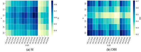
Figure 3.
Grid search results for the SI and DBI indices. (a) SI; (b) DBI.
Table 3.
The details of itemsets for mining association rules.
4.3. Results of Trajectory Structure Characterization
Figure 4 visualizes the detected abnormal trajectories; additionally, all trajectories and normal trajectories are also shown for ease of comparison. The abnormal trajectories account for 21.3% of all observations, and are treated as spatial anomalies. On the whole, the regular parts or frequently used paths of all trajectories are retained in the normal trajectories, while those with fewer occurrences are summarized in the abnormal trajectories. Although some abnormal trajectories seem to show a spatial structure formed by normal trajectories to a certain extent, by further applying the automatic holding pattern detection algorithm proposed by [22] to these trajectories, it is found that 92.13% of them have holding patterns (i.e., one or more self-intersecting segments), which are distributed in the east and south sides of the map, respectively. This phenomenon effectively validates the performance of the proposed anomaly detection method since they are treated as structured anomalies, which are often associated with ATC actions.
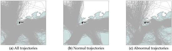
Figure 4.
Results of abnormal-trajectory detection. (a) All trajectories; (b) Normal trajectories; (c) Abnormal trajectories.
After finding abnormal trajectories from sparse matrix , the normal trajectories in are used to learn cluster-friendly representations, on which cluster analysis is performed to obtain their cluster assignments. Figure 5 gives the trajectory spatial clustering results corresponding to the best SI and DBI. As can be seen from Figure 5b,c, a total of 12 clusters are formed in the Hong Kong terminal area, of which the trajectories from the east form the two most mainstream clusters, accounting for 26.92% and 10.60% of the observations, respectively. Moreover, trajectories from the southwest and southeast also form two clusters corresponding to different runway configurations. In comparison, the routes of trajectories from the northwest and north are more complex and changeable, each forming three clusters. In order to further analyze the distribution of each cluster, the t-SNE visualization technique [29] is applied by projecting the fifty-dimensional representation space into two-dimensional space. As shown in Figure 5d, each point represents a trajectory with a color as its cluster label. It can be intuitively seen that some of the clusters exhibit good intrinsic compactness and extrinsic separability, which reflects the finding that the proposed methods can effectively learn a cluster-friendly space. However, there is overlap in the distributions of some clusters (such as those formed by trajectories from the northwest and north). This phenomenon is caused by the high similarity between trajectories on the one hand and the optimization goal on the other. As can be seen from Equation (7), the objective function needs to take into account both the trajectory reconstruction ability and cluster compactness.
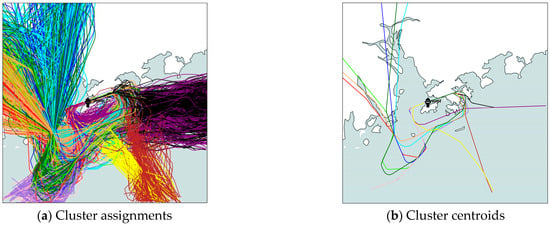
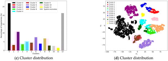
Figure 5.
Results of trajectory spatial clustering.
4.4. Results of Flow Pattern Recognition
With the cluster assignment results of trajectories in mind, a more macroscopic view of the changes in airspace structure over time can be obtained. Figure 6 visualizes the per-hour-level description vectors for both months, including a total of 1464 h, for which the color reflects the number of flights belonging to each cluster or spatial anomalies. It can be seen that some clusters, such as cluster 0 and cluster 2 (corresponding to trajectories from the east), usually do not appear at the same time, mainly due to the constraints of runway configuration in airport operations. In addition, some clusters (such as cluster 8) appear cyclically over a period of time due to flight schedules. Based on the number of flights with spatial anomalies, it is possible to initially understand the complexity and uncertainty of the operating situation in the terminal airspace. All of the above valuable knowledge can be obtained from such a compressed representation (and not necessarily specific trajectory information) to more intuitively monitor and perceive the spatio-temporal characteristics of tactical operations. Furthermore, from Figure 5c and Figure 6a, it can be concluded that the distribution of each cluster is uneven, regardless of the overall scope or hourly granularity. To reduce the sensitivity of the Euclidean distance-based similarity calculation to factor scaling in the DBSCAN algorithm, each dimension is mapped to [0, 1] through the min–max normalization technique, as shown in Figure 6b.
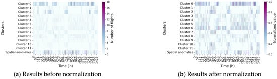
Figure 6.
Temporal distribution of spatial structure utilization before and after normalization.
Based on the normalized description vectors, a total of 10 flow patterns were recognized by the DBSCAN clustering algorithm. Figure 7 gives the centroids of each pattern, along with their respective proportions. It can be determined that the different flow patterns are highly discriminative, and a few patterns can capture the majority of observations. A more intuitive visualization result of flow patterns is shown in Figure 8, in which the shade of color reflects the number of flights in each spatial cluster. For analytical convenience, the top six flow patterns, accounting for nearly 80% of the observations, were selected to preliminarily understand the characteristics of the arrival flow in the Hong Kong TMA.
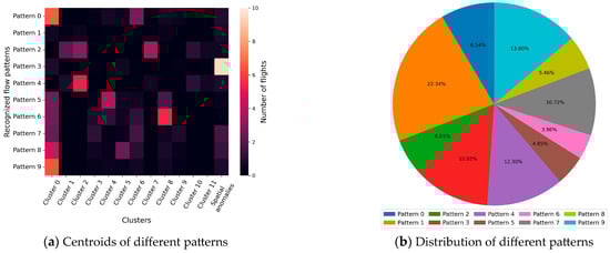
Figure 7.
Results of flow pattern recognition.
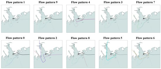
Figure 8.
Visualization of flow patterns (from high frequency to low frequency).
Based on the number of main spatial clusters, Table 4 categorizes the dominant patterns and summarizes their detailed descriptions. It can be roughly inferred that flight distribution, runway configuration, and spatial anomalies are direct factors influencing and driving flow pattern changes. For instance, both pattern 9 and pattern 4 capture the east spatial cluster (i.e., trajectories from the east), but differ due to the use of runway configuration. Moreover, as observed in Figure 8, flow pattern 1 and flow pattern 3 are similar, and both are mixed spatial clusters (i.e., each cluster has few flights). In fact, compared to flow pattern 1, a large number of trajectories in flow pattern 3 are classified as spatial anomalies (see pattern 1 and pattern 3 in Figure 7a). As for flow pattern 1, preliminary statistics show that most of its description vectors come from the early morning periods when arrival demand is usually less. Essentially, the above factors affecting flow patterns are highly correlated with the dynamic and variable weather conditions in the TMA. For example, the selected runway configuration for arrival flights is mainly determined by the wind direction and speed. For safety and operational reasons, aircraft usually land against the wind. Visual meteorological conditions (VMC) and instrument meteorological conditions (IMC) have also been empirically associated with runway selection [8], indirectly reflecting the effects of visibility and clouds. Additionally, the presence of convective weather will force some typical spatial anomalies in trajectory behavior, such as holding pattern and traffic rerouting, which in turn affect the spatial distribution of flights.
Table 4.
Description of dominant (top six) arrival flow patterns in the Hong Kong TMA.
4.5. Analysis of Association Rules between Traffic Flows and Weather Factors
Before mining association rules, based on minimum support of 1%, the set of items that frequently occur together (i.e., frequent itemsets) are searched; Figure 9 presents the corresponding results. A total of 1,096,785 itemsets are found, of which Figure 9a shows the itemsets corresponding to the top-10-highest support values, and Figure 9b counts the number of itemsets with different itemset sizes. It can be inferred that although June and July are the most active periods of convective weather in Hong Kong, extreme weather conditions such as thunderstorms, wind shear, and cumulonimbus rarely occur, and the visibility is greater than 8 km in most periods. Based on such characteristics, in the subsequent analysis of association rules, the minimum threshold for support is also set to 1% to ensure that the rules related to extreme weather can be captured. Additionally, due to the low support threshold, a large number of itemsets are considered frequent, and the number of itemsets reaches a maximum when the size of the itemset is 7 or 8. Considering the scale of the itemsets and previous studies, this paper mainly analyzes the association rules associated with itemset sizes of 2 to 4.
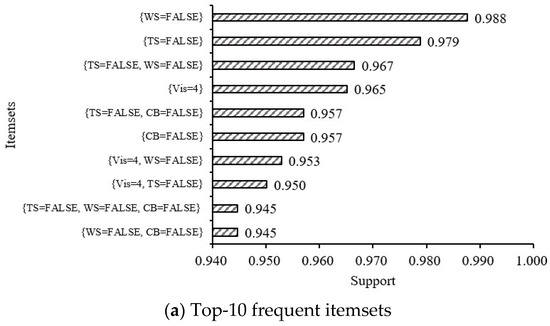

Figure 9.
Results of frequent-itemsets searching.
Taking 1%, 15%, and 1.5 as the minimum thresholds for support, confidence, and lift, Table 5, Table 6, Table 7, Table 8 and Table 9 show the two-item, three-item, and four-item association rules, with the dominant (top six) arrival flow patterns as the consequent, respectively. All rules are sorted in descending order of the lift indicator, and the top 10 rules of each category are displayed (if they exist). Each Rule ID consists of the flow pattern ID, the number of antecedents, and the local rank. Overall, it can be found that regardless of flow pattern, the lift of four-item association rules is usually larger than those of the three-item and the two-item, and the lift of three-item association rules is usually larger than that of the two-item. This phenomenon fully indicates that each flow pattern is affected by multiple factors, and its formation is the result of the complex interaction among different factors. In the following subsections, we focus on analyzing how meteorological factors affect the three types of flow patterns mentioned in Table 4.
4.5.1. Case 1: Analysis of Traffic Flows with No Main Spatial Cluster
Since patterns 1 and 3 belong to traffic flows with no main spatial cluster, for the convenience of comparison, their two-item, three-item, and four-item association rules are given, respectively, as shown in Table 5 and Table 6. In the two-item association rule, the important rule for pattern 1 is related to the busy hour, while the important rule for pattern 3 is related to cumulonimbus strong winds, rain, etc. Since the difference between the two patterns is the number of flights and abnormal trajectories (see Table 4), these rules are easy to understand. Rule 1-1-1 indicates that if the current traffic is not during a busy hour, the flow structure of the airspace is likely to be pattern 1. Likewise, Rules 3-1-1 to 3-1-5 reflect that the busy hour or the presence of weather phenomena such as cumulonimbus and strong winds are more likely to drive the formation of flow pattern 3.
Table 5.
Two-item association rules with respect to flow patterns 1 and 3.
Table 5.
Two-item association rules with respect to flow patterns 1 and 3.
| Rule ID | Association Rules | Measures | |||
|---|---|---|---|---|---|
| LHS | RHS | Support | Confidence | Lift | |
| 1-1-1 | Bh = False | F_p = 1 | 0.143 | 0.384 | 1.717 |
| 3-1-1 | CB = True | F_p = 3 | 0.015 | 0.349 | 2.905 |
| 3-1-2 | Ws > 15KT | 0.021 | 0.300 | 2.504 | |
| 3-1-3 | RA = True | 0.024 | 0.217 | 1.808 | |
| 3-1-4 | Ws = 12–15KT | 0.027 | 0.206 | 1.716 | |
| 3-1-5 | Bh = True | 0.121 | 0.193 | 1.603 | |
Table 6.
Three-item and four-item association rules with respect to flow patterns 1 and 3.
Table 6.
Three-item and four-item association rules with respect to flow patterns 1 and 3.
| Rule ID | Association Rules | Measures | ||||
|---|---|---|---|---|---|---|
| LHS | RHS | Support | Confidence | Lift | ||
| Three-item rules | 1-2-1 | Bh = False & Wd = 90–180° | F_p = 1 | 0.033 | 0.438 | 1.959 |
| 1-2-2 | Bh = False & Wd = 0–90° | 0.029 | 0.429 | 1.919 | ||
| 1-2-3 | Bh = False & Ws = 3–6KT | 0.048 | 0.428 | 1.915 | ||
| 1-2-4 | Bh = False & We = False | 0.099 | 0.422 | 1.887 | ||
| 1-2-5 | Bh = False & Vis > 8 km | 0.132 | 0.412 | 1.842 | ||
| 1-2-6 | Bh = False & RA = False | 0.122 | 0.411 | 1.838 | ||
| 1-2-7 | Bh = False & Wdc = False | 0.066 | 0.408 | 1.825 | ||
| 1-2-8 | Bh = False & CB = False | 0.130 | 0.407 | 1.823 | ||
| 1-2-9 | Bh = False & Ceiling = 300–900 m | 0.018 | 0.406 | 1.819 | ||
| 1-2-10 | Bh = False & TS = False | 0.133 | 0.405 | 1.813 | ||
| 3-2-1 | Bh = True & CB = True | F_p = 3 | 0.015 | 0.500 | 4.159 | |
| 3-2-2 | RA = True & CB = True | 0.011 | 0.421 | 3.502 | ||
| 3-2-3 | Ceiling = 150–300 m & CB = True | 0.014 | 0.362 | 3.012 | ||
| 3-2-4 | Ws > 15KT & Cover = SCT | 0.015 | 0.349 | 2.905 | ||
| 3-2-5 | Cover = SCT & CB = True | 0.013 | 0.345 | 2.874 | ||
| 3-2-6 | Bh = True & Ws > 15KT | 0.021 | 0.333 | 2.773 | ||
| 3-2-7 | Ws > 15KT & Ceiling = 150–300 m | 0.020 | 0.330 | 2.741 | ||
| 3-2-8 | Bh = True & RA = True | 0.024 | 0.321 | 2.671 | ||
| 3-2-9 | Wd = 180–270° & Ws > 15KT | 0.012 | 0.305 | 2.538 | ||
| 3-2-10 | Wd = 180–270° & RA = True | 0.014 | 0.299 | 2.483 | ||
| Four-item rules | 1-3-1 | Bh = False & Wd = 0–90° & Ws = 3–6KT | F_p = 1 | 0.013 | 0.543 | 2.430 |
| 1-3-2 | Bh = False & Wd = 0–90° & Cover = FEW | 0.018 | 0.491 | 2.198 | ||
| 1-3-3 | Bh = False & We = False & Wd = 90–180° | 0.027 | 0.471 | 2.107 | ||
| 1-3-4 | Bh = False & Ws = 3–6KT & Wdc = False | 0.022 | 0.464 | 2.076 | ||
| 1-3-5 | Bh = False & Wd = 0–90° & RA = False | 0.027 | 0.459 | 2.054 | ||
| 1-3-6 | Bh = False & We = False & Ceiling = 300–900 m | 0.014 | 0.455 | 2.035 | ||
| 1-3-7 | Bh = False & Wd = 0–90° & Wdc = False | 0.023 | 0.453 | 2.030 | ||
| 1-3-8 | Bh = False & Wd = 90–180° & Ws = 3–6KT | 0.015 | 0.449 | 2.010 | ||
| 1-3-9 | Bh = False & We = False & Cover = FEW | 0.055 | 0.444 | 1.990 | ||
| 1-3-10 | Bh = False & Wd = 0–90° & Vis > 8 km | 0.029 | 0.442 | 1.979 | ||
| 3-3-1 | Bh = True & CB = True & RA = True | F_p = 3 | 0.011 | 0.593 | 4.930 | |
| 3-3-2 | Bh = True & CB = True & Ceiling = 150–300 m | 0.014 | 0.525 | 4.367 | ||
| 3-3-3 | Bh = True & CB = True & Cover = SCT | 0.013 | 0.514 | 4.272 | ||
| 3-3-4 | Ws > 15KT & Ceiling = 150–300 m & Pre < 1005 hPa | 0.017 | 0.455 | 3.781 | ||
| 3-3-5 | Bh = True & Wd = 180–270° & RA = True | 0.014 | 0.455 | 3.781 | ||
| 3-3-6 | Bh = True & Wd = 180–270° & Ws > 15KT | 0.012 | 0.448 | 3.722 | ||
| 3-3-7 | Bh = True & Ws > 15KT & Pre < 1005 hPa | 0.018 | 0.433 | 3.605 | ||
| 3-3-8 | Ceiling = 150–300 m & CB = True & Pre < 1005 hPa | 0.010 | 0.429 | 3.565 | ||
| 3-3-9 | Bh = True & Wd = 180–270° & Ws = 12–15KT | 0.018 | 0.415 | 3.448 | ||
| 3-3-10 | Ceiling = 150–300 m & CB = True & RA = True | 0.010 | 0.405 | 3.372 | ||
As for the three-item association rules, the combination of different factors forms more rules. For pattern 1, the non-busy hour and various favorable weather conditions constitute the majority of the antecedents. Since these periods are protected from severe weather, the number of trajectories that are spatially anomalous is small. In addition, based on Rules 1-2-1 and 1-2-2, it can be inferred that specific wind directions during non-busy hours are also likely to induce the appearance of pattern 1. Compared with pattern 1, the antecedents of pattern 3 are more a combination of a busy hour and severe weather (e.g., Rules 3-2-1, 3-2-6, and 3-2-8) or a combination of various weather factors (e.g., Rules 3-2-2, 3-2-3, and 3-2-7). In order to avoid areas covered by cumulonimbus or extreme rainfall, the trajectory needs to change its original route. More importantly, due to the unbalanced capacity and demand of airports caused by complex meteorological conditions in busy hours, arriving flights often cannot immediately land, and have to stay in holding patterns. As a result of the above-mentioned diverse trajectory behaviors, there are a large number of spatial anomalies in the terminal airspace. Another interesting phenomenon is that strong winds from a certain direction (i.e., 180–270°) also have a high probability of driving the appearance of pattern 3 (Rule 3-2-9). The reason may be that there will be more changes in trajectory behavior under such conditions, resulting in more diverse abnormal trajectories. This phenomenon also occurs in pattern 7 (Rule 7-2-6) and pattern 9 (Rule 9-2-3).
Four-item association rules also obtain conclusions similar to those of two-item and three-item association rules. In particular, Rules 1-3-2 and 1-3-9 reveal that the characteristic of cloud cover affecting pattern 1 is that of few clouds. And the importance of strong winds from the direction of 180–270° for pattern 3 is further verified by Rules 3-3-6 and 3-3-9.
4.5.2. Case 2: Analysis of Traffic Flows with One Main Spatial Cluster
Pattern 4 and pattern 9 are the two recognized major patterns that belong to traffic flows with one main spatial cluster (i.e., the east spatial cluster). Accordingly, their respective two-item, three-item, and four-item association rules are compared in Table 7 and Table 8. It can be clearly determined from the two-item association rules that the wind direction is the most critical factor affecting these two patterns. When the airport traffic is affected by an east wind, the runway configuration for arrival flights is usually set to 07C; hence, the flights are scheduled to land from the southwest. Conversely, when the airport is affected by a west wind, the runway configuration for arrival flights is usually set to 25C; hence, the flights are scheduled to land from the northeast.
Table 7.
Two-item association rules with respect to flow patterns 4 and 9.
Table 7.
Two-item association rules with respect to flow patterns 4 and 9.
| Rule ID | Association Rules | Measures | |||
|---|---|---|---|---|---|
| LHS | RHS | Support | Confidence | Lift | |
| 4-1-1 | Wd = 90–180° | F_p = 4 | 0.065 | 0.300 | 2.437 |
| 4-1-2 | Wd = 0–90° | 0.044 | 0.256 | 2.081 | |
| 9-1-1 | Wd = 180–270° | F_p = 9 | 0.102 | 0.212 | 1.538 |
Table 8.
Three-item and four-item association rules with respect to flow patterns 4 and 9.
Table 8.
Three-item and four-item association rules with respect to flow patterns 4 and 9.
| Rule ID | Association Rules | Measures | ||||
|---|---|---|---|---|---|---|
| LHS | RHS | Support | Confidence | Lift | ||
| Three-item rules | 4-2-1 | Wd = 90–180° & Ws = 9–12KT | F_p = 4 | 0.023 | 0.379 | 3.085 |
| 4-2-2 | Wd = 90–180° & Bh = True | 0.048 | 0.341 | 2.777 | ||
| 4-2-3 | Wd = 90–180° & Ceiling < 150 m | 0.012 | 0.333 | 2.711 | ||
| 4-2-4 | Wd = 0–90° & Ws = 6–9KT | 0.016 | 0.324 | 2.635 | ||
| 4-2-5 | Wd = 90–180° & Vis > 8 km | 0.065 | 0.309 | 2.517 | ||
| 4-2-6 | Wd = 90–180° & Cover = SCT | 0.029 | 0.309 | 2.512 | ||
| 4-2-7 | Wd = 90–180° & CB = False | 0.064 | 0.304 | 2.472 | ||
| 4-2-8 | Wd = 90–180° & RA = False | 0.058 | 0.302 | 2.460 | ||
| 4-2-9 | Wd = 90–180° & TS = False | 0.064 | 0.301 | 2.448 | ||
| 4-2-10 | Wd = 90–180° & WS = False | 0.065 | 0.301 | 2.445 | ||
| 9-2-1 | Wd = 180–270° & Ceiling = 300–900 m | F_p = 9 | 0.015 | 0.296 | 2.405 | |
| 9-2-2 | We = True & Ws = 12–15KT | 0.046 | 0.296 | 2.405 | ||
| 9-2-3 | Wd = 180–270° & Ws = 12–15KT | 0.038 | 0.288 | 2.342 | ||
| 9-2-4 | Wd = 180–270° & Bh = True | 0.017 | 0.287 | 2.337 | ||
| 9-2-5 | Wd = 180–270° & Cover = FEW | 0.023 | 0.276 | 2.248 | ||
| 9-2-6 | Wd = 180–270° & RA = False | 0.011 | 0.262 | 1.901 | ||
| Four-item rules | 4-3-1 | Wd = 90–180° & Ws = 9–12KT & T < 30 °C | F_p = 4 | 0.013 | 0.559 | 4.545 |
| 4-3-2 | Wd = 90–180° & Bh = True & T < 30 °C | 0.019 | 0.424 | 3.451 | ||
| 4-3-3 | Wd = 90–180° & Cover = SCT & Pre < 1005 hPa | 0.013 | 0.413 | 3.359 | ||
| 4-3-4 | Wd = 0–90° & Ws = 6–9KT & Ceiling = 150–300 m | 0.014 | 0.400 | 3.253 | ||
| 4-3-5 | We = True & Dp < 24 °C & RA = False | 0.013 | 0.396 | 3.219 | ||
| 4-3-6 | We = True & Bh = True & Dp < 24 °C | 0.011 | 0.390 | 3.174 | ||
| 4-3-7 | Wd = 90–180° & Ws = 9–12KT & CB = False | 0.023 | 0.389 | 3.162 | ||
| 4-3-8 | Wd = 90–180° & Ws = 9–12KT & Vis > 8 km | 0.023 | 0.388 | 3.158 | ||
| 4-3-9 | Wd = 90–180° & Ws = 9–12KT & TS = False | 0.023 | 0.388 | 3.158 | ||
| 4-3-10 | Wd = 90–180° & Ws = 9–12KT & RA = False | 0.021 | 0.387 | 3.151 | ||
| 9-3-1 | Wd = 180–270° & Ws = 12–15KT & We = True | F_p = 9 | 0.011 | 0.333 | 2.416 | |
| 9-3-2 | Ws = 12–15KT & We = True & Dp ≥ 24 °C | 0.012 | 0.327 | 2.369 | ||
| 9-3-3 | Ws = 12–15KT & We = True & T ≥ 30 °C | 0.012 | 0.304 | 2.200 | ||
| 9-3-4 | Wd = 180–270° & Ceiling = 300–900 m &RA = False | 0.011 | 0.286 | 2.071 | ||
| 9-3-5 | Wd = 180–270° & Vis > 8 km & Ceiling = 300–900 m | 0.011 | 0.271 | 1.965 | ||
| 9-3-6 | Ws = 12–15KT & We = True & CB = False | 0.012 | 0.269 | 1.947 | ||
| 9-3-7 | Wd = 180–270° & Ceiling = 300–900 m &CB = False | 0.011 | 0.267 | 1.933 | ||
| 9-3-8 | Wd = 180–270° & Ceiling = 300–900 m &TS = False | 0.011 | 0.267 | 1.933 | ||
| 9-3-9 | Wd = 180–270° & Ws = 12–15KT & Cover = SCT | 0.012 | 0.266 | 1.925 | ||
| 9-3-10 | Ws = 12–15KT & We = True & Vis > 8 km | 0.012 | 0.265 | 1.918 | ||
Aside from wind direction, wind speed, cloud ceiling, and cloud cover are also key weather factors affecting patterns, a finding which can be inferred from the three-item and four-item association rules. Rules 4-2-1 and 4-2-4 suggest that easterly winds of 6–12KT are more likely to form flow pattern 4, while Rules 9-2-3, 9-3-1, and 9-3-9 give strong evidence that westerly winds of 12–15KT are more likely to drive flow pattern 9. Although both patterns have relatively strong winds during busy periods, the number of trajectories that are spatially anomalous is not large, due to high visibility (Rules 4-2-5 and 9-3-5) and favorable meteorological conditions (Rules 4-2-7 to 4-2-10 and Rules 9-3-7 to 9-3-8). In addition, the characteristics of the cloud are also different in the two patterns. Scattered clouds (Rules 4-2-6 and 4-3-3) and a ceiling of less than 300m (Rules 4-2-3 and 4-3-4) are more likely to affect pattern 4, while a ceiling of more than 300 m (Rules 9-2-1 and 9-3-5) is more likely to affect pattern 9.
4.5.3. Case 3: Analysis of Traffic Flows with Multiple Main Spatial Clusters
Pattern 0 and pattern 7 are the two recognized major patterns that belong to traffic flows with multiple main spatial clusters (i.e., the southwest and east spatial clusters are associated with pattern 0, while the southwest, northwest, and east spatial clusters are associated with pattern 7). Since there is no two-item association rule that meets the minimum threshold requirement for the two patterns, only the comparison of the respective three-item and four-item association rules is given in Table 9. Among the discovered association rules, the two patterns are generally similar, but individuals have some differences.
Table 9.
Three-item and four-item association rules with respect to flow patterns 0 and 7.
Table 9.
Three-item and four-item association rules with respect to flow patterns 0 and 7.
| Rule ID | Association Rules | Measures | ||||
|---|---|---|---|---|---|---|
| LHS | RHS | Support | Confidence | Lift | ||
| Three-item rules | 0-2-1 | Bh = True & Ceiling < 150 m | F_p = 0 | 0.020 | 0.182 | 2.136 |
| 0-2-2 | We = True & Ceiling < 150 m | 0.011 | 0.172 | 2.015 | ||
| 0-2-3 | Wd = 180–270° & Ceiling < 150 m | 0.015 | 0.162 | 1.895 | ||
| 0-2-4 | Wd = 180–270° & Cover = FEW | 0.043 | 0.154 | 1.808 | ||
| 0-2-5 | Ws = 9–12KT & Cover = FEW | 0.018 | 0.153 | 1.797 | ||
| 0-2-6 | Wd = 180–270° & Ws = 9–12KT | 0.025 | 0.153 | 1.791 | ||
| 7-2-1 | Wd = 180–270° & Bh = True | F_p = 7 | 0.066 | 0.188 | 1.753 | |
| 7-2-2 | Bh = True & TS = True | 0.014 | 0.185 | 1.725 | ||
| 7-2-3 | Bh = True & Ceiling < 150 m | 0.019 | 0.176 | 1.642 | ||
| 7-2-4 | Bh = True & Ws = 9–12KT | 0.028 | 0.164 | 1.529 | ||
| 7-2-5 | Bh = True & Cover = FEW | 0.058 | 0.164 | 1.527 | ||
| 7-2-6 | Wd = 180–270° & Ws = 12–15KT | 0.014 | 0.162 | 1.512 | ||
| Four-item rules | 0-3-1 | We = True & Bh = True & Ceiling < 150 m | F_p = 0 | 0.010 | 0.234 | 2.745 |
| 0-3-2 | Wd = 180–270° & Ws = 9–12KT & Cover = FEW | 0.018 | 0.215 | 2.517 | ||
| 0-3-3 | Bh = True & Ceiling = 150–300 m & Pre ≥ 1005 hPa | 0.015 | 0.208 | 2.431 | ||
| 0-3-4 | Wd = 180–270° & Bh = True & Ceiling < 150 m | 0.014 | 0.206 | 2.415 | ||
| 0-3-5 | Ceiling < 150 m & T ≥ 30 °C & Pre ≥ 1005 hPa | 0.011 | 0.200 | 2.342 | ||
| 0-3-6 | Wd = 180–270° & Ws = 9–12KT & Bh = True | 0.023 | 0.194 | 2.274 | ||
| 0-3-7 | Wd = 180–270° & Bh = True & Cover = FEW | 0.038 | 0.193 | 2.262 | ||
| 0-3-8 | Bh = True & Ceiling < 150 m & T ≥ 30 °C | 0.015 | 0.190 | 2.221 | ||
| 0-3-9 | Wd = 180–270° & Ceiling < 150 m & T ≥ 30 °C | 0.013 | 0.188 | 2.203 | ||
| 0-3-10 | Bh = True & Ceiling < 150 m & RA = False | 0.020 | 0.187 | 2.191 | ||
| 7-3-1 | Bh = True & Ceiling < 150 m & T ≥ 30 °C | F_p = 7 | 0.016 | 0.207 | 1.929 | |
| 7-3-2 | Bh = True & Ws = 9–12KT & Wdc = False | 0.018 | 0.206 | 1.924 | ||
| 7-3-3 | Bh = True & Wd = 180–270° & T ≥ 30 °C | 0.064 | 0.206 | 1.922 | ||
| 7-3-4 | Bh = True & Wd = 180–270° & Ceiling = 150–300 m | 0.052 | 0.201 | 1.870 | ||
| 7-3-5 | Bh = True & Wd = 180–270° & Cover = FEW | 0.040 | 0.200 | 1.865 | ||
| 7-3-6 | Bh = True & Wd = 180–270° & Wdc = False | 0.042 | 0.198 | 1.847 | ||
| 7-3-7 | Ws = 9–12KT & Wdc = False & T ≥ 30 °C | 0.017 | 0.195 | 1.821 | ||
| 7-3-8 | Bh = True & Wd = 180–270° & Dp ≥ 24 °C | 0.066 | 0.193 | 1.801 | ||
| 7-3-9 | Bh = True & Wd = 180–270° & TS = True | 0.010 | 0.192 | 1.791 | ||
| 7-3-10 | Bh = True & Wd = 180–270° & WS = True | 0.010 | 0.190 | 1.772 | ||
Specifically, Rules 0-2-1 and 7-2-3 reflect the fact that poor visual conditions during busy hours are more likely to drive the forming of these two patterns. When the cloud ceiling is less than 150 m, aircrafts have to fly under the IFR rules, and air traffic controllers will step in and guide pilots along the established air routes, which may lead to seemingly “abnormal” trajectory behavior in the airspace. Additionally, Rules 0-2-6 and 7-2-6 indicate that strong winds from the direction of 180–270° are also likely to cause these two patterns to appear. This is because this condition directly affects the setting of the runway configuration, which is set to 25C for safety and operational reasons. In particular, differing from pattern 0, the occurrence of thunderstorms or wind shear is also likely to drive the occurrence of pattern 7, which can be confirmed by Rules 7-2-2, 7-3-9, and 7-3-10. Due to such extreme weather conditions, the behavior of more trajectories is restricted. Based on preliminary statistics, flights from the east are the most affected, and a large portion of them are identified as abnormal trajectories, resulting in the formation of pattern 7 with multiple main spatial clusters.
4.5.4. Identification of Important Factor Combinations for Dominant Arrival Flow Patterns
To better identify the key factors affecting different flow patterns, a group matrix-based visualization technique [44] is applied, in which the antecedents of different rules are grouped by clustering, and the rules are sorted by “interestingness” (“lift” is used in this paper). Figure 10 visualizes the grouped matrix of the two-item, three-item, and four-item association rules, respectively, which is a balloon plot with each grouped antecedent as a column and each consequent as a row. The color of the balloon represents the aggregated lift in the group, and the size of the balloon indicates the aggregated support. Here, both metrics are measured by the within-group median. A small, dark balloon means that the group of rules has a lower frequency of occurrence but higher interest and value, and a large, shallow balloon means that the group of rules has relatively lower interest and value but a higher frequency of occurrence.
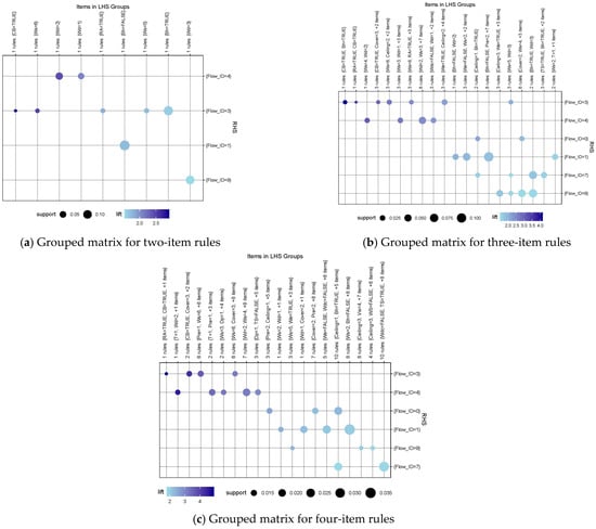
Figure 10.
Visualizations of important factor combinations based on grouped matrix.
As can be seen from Figure 10, on the whole, the antecedents corresponding to different flow patterns are often different. As for flow pattern 3, it has the factor combinations with the highest number and highest interest as antecedents. This may be due to the nature of its massive abnormal trajectories, which far exceed the scale of other patterns. Among all meteorological factors, cumulonimbus, strong winds, and rain are the three most important influencing factors. In addition, the combination of them, or their respective co-occurrences with busy periods, low cloud ceiling, high cloud cover, etc., will further promote the formation of pattern 3. In contrast, non-busy hours and the combination of this condition with favorable weather conditions are the main factors in the formation of pattern 1, and the combination of low wind speed and easterly wind, and their respective combinations with non-busy periods, are the most important, including a total of 13 rules.
In terms of pattern 4, easterly winds and its combinations with relatively high wind speeds are the most important factors. Especially when the two are combined, the probability of pattern 4 appearing is greatly increased. In the three-item and four-item grouped matrices, there are 12 and 7 rules related to this kind of combination, respectively. And as for pattern 9, having easterly winds is the most important factor. Among the factor combinations, the most important are weekend day and high cloud ceiling, weekend day and high wind speeds, and easterly winds and high wind speeds, all of which correspond to three rules. As for pattern 0 and pattern 7, low cloud ceiling and busy hours is their most important factor combination, involving a total of 12 rules. However, they also have some different factor combinations. For example, the combination of low cloud cover and relatively high wind speeds is important for pattern 0, while the combination of busy hours and thunderstorm is important for pattern 7.
It is precisely because of the differences in the combinations of factors that a diverse traffic flow pattern is formed. With the extracted valuable information and the report of the terminal-area forecast (TAF) in mind, it is easier to perceive the airspace operation situation and predict the traffic flow pattern in advance.
5. Conclusions
The use of big data analytics to aid decision-making in air traffic management is an emerging concept. In order to understand the impact of meteorological conditions on air traffic behavior, a data-driven intelligent analysis framework is proposed, which includes three progressive modules, namely, trajectory structure characterization, flow pattern recognition, and association rule mining. To capture the spatial structure of trajectories, a deep autoencoder network based on row sparsity and KL divergence is sequentially applied to achieve decoupling between cluster analysis and anomaly detection. To further identify the spatio-temporal patterns of traffic flow, a cluster analysis is performed using the DBSCAN algorithm on a compressed representation that describes airspace usage. Based on the identified major traffic flow patterns and diverse meteorological factors, the apriori algorithm is used to construct two-item, three-item, and four-item association rules to discover useful factor combinations affecting the patterns. The potential and value of the proposed framework are validated using real data from the Hong Kong International Airport over a two-month period. It can not only effectively strip out abnormal trajectories from all trajectories and obtain discriminative spatial clusters, but also capture representative spatio-temporal properties of air traffic flow. The valuable knowledge and typical patterns extracted through multimodal analysis can assist in the formulation of an airspace use plan and the construction of an airspace capacity model, which is helpful for central flow traffic planning and management. In addition, by analyzing numerous association rules, it is found that different patterns are driven by different combinations of factors. In particular, the combination of severe weather factors directly brings about a large number of spatial anomalous trajectories, which in turn affects the formation of patterns. In addition, the combination of wind direction and wind speed is also one of the representative combinations, one which affects the pattern by changing the runway configuration.
Future work will focus on the following topics:
- (1)
- Establishing a prediction model of air traffic flow patterns with time series characteristics based on each meteorological factor and its combinations, aiming to enrich this weather-related decision support tool for ATM.
- (2)
- Analyzing the association between the forecasted weather obtained from Terminal Aerodrome Forecasts (TAF) and traffic flow patterns, and then comparing the differences in association rules between the two types of weather (i.e., METAR vs. TAF).
- (3)
- Determining how to deal with the potential noise brought by other non-meteorological factors to the analysis process is also an interesting topic. Taking various factors into account or estimating the impact of such noise is a research perspective worthy of further attempts.
Author Contributions
Conceptualization, W.Z. and J.D.; methodology, W.Z. and J.Y.; software, W.Z. and J.D.; validation, W.Z., J.D. and J.Y.; formal analysis, J.D.; investigation, W.Z. and J.D.; resources, W.Z.; data curation, W.Z.; writing—original draft preparation, W.Z. and J.D.; writing—review and editing, W.Z. and J.D.; visualization, W.Z. and J.D.; supervision, W.P. and X.Z.; project administration, W.P.; funding acquisition, W.P., C.Y., X.Z. and J.Y. All authors have read and agreed to the published version of the manuscript.
Funding
This research was co-supported by the National Key R&D Program of China (2021YFB2601704), the Joint Funds of the National Natural Science Foundation of China (U2333209), the National Natural Science Foundation of China (No. 52002178), the Sichuan Science and Technology Program (2023YFSY0025), and the Fundamental Research Funds for the Central Universities (ZHMH2022-008).
Data Availability Statement
Data are contained within the article.
Acknowledgments
We would like to thank the OpenSky Network for providing rich APIs to help the authors collect the ADS-B flight trajectories data used in this paper.
Conflicts of Interest
The authors declare no conflicts of interest.
References
- Du, J.; Hu, M.; Zhang, W.; Yin, J. Finding Similar Historical Scenarios for Better Understanding Aircraft Taxi Time: A Deep Metric Learning Approach. IEEE Intell. Transp. Syst. Mag. 2022, 15, 101–116. [Google Scholar] [CrossRef]
- Lui, G.N.; Hon, K.K.; Liem, R.P. Weather impact quantification on airport arrival on-time performance through a Bayesian statistics modeling approach. Transp. Res. Part C Emerg. Technol. 2022, 143, 103811. [Google Scholar] [CrossRef]
- Arneson, H.; Bombelli, A.; Segarra-Torné, A.; Tse, E. Analysis of convective-weather impact on pre-departure routing decisions for flights traveling between Fort Worth Center and New York Air Center. In Proceedings of the 17th AIAA Aviation Technology, Integration, and Operations Conference, Denver, CO, USA, 5–9 June 2017. [Google Scholar] [CrossRef]
- Lui, G.N.; Liem, R.P.; Hon, K. Towards understanding the impact of convective weather on aircraft arrival traffic at the Hong Kong International Airport. In Proceedings of the 2020 The Third International Workshop on Environment and Geoscience, Chengdu, China, 18–20 July 2020; IOP Publishing: Bristol, UK, 2020; Volume 569. [Google Scholar] [CrossRef]
- Olive, X.; Grignard, J.; Dubot, T.; Saint-Lot, J. Detecting Controllers’ Actions in Past Mode S Data by Autoencoder-Based Anomaly Detection. In Proceedings of the 8th SESAR Innovation Days, Salzburg, Austria, 3–7 December 2018. [Google Scholar]
- Murca, M.C.R.; DeLaura, R.; Hansman, R.J.; Jordan, R.; Reynolds, T.; Balakrishnan, H. Trajectory clustering and classification for characterization of air traffic flows. In Proceedings of the 16th AIAA Aviation Technology, Integration, and Operations Conference, Washington, DC, USA, 13–17 June 2016. [Google Scholar] [CrossRef]
- Lemetti, A.; Polishchuk, T.; Polishchuk, V.; Sáez García, R.; Prats Menéndez, X. Identification of significant impact factors on Arrival Flight Efficiency within TMA. In Proceedings of the ICRAT 2020, Virtual Event, 15 September 2020; pp. 1–8. [Google Scholar]
- Liu, Y.L.; Hansen, M.; Lovell, D.J.; Chuang, C.; Ball, M.O.; Gulding, J.M. Causal analysis of en route flight inefficiency-the US experience. In Proceedings of the Twelfth USA/Europe Air Traffic Management Research and Development Seminar, Seattle, WA, USA, 26–30 June 2017; Volume 570. [Google Scholar]
- Rodríguez-Sanz, Á.; Cano, J.; Rubio Fernandez, B. Impact of Weather Conditions on Airport Arrival Delay and Throughput. Aircr. Eng. Aerosp. Technol. 2022, 94, 60–78. [Google Scholar] [CrossRef]
- Olive, X.; Basora, L. Detection and identification of significant events in historical aircraft trajectory data. Transp. Res. Part C Emerg. Technol. 2020, 119, 102737. [Google Scholar] [CrossRef]
- Gariel, M.; Srivastava, A.N.; Feron, E. Trajectory clustering and an application to airspace monitoring. IEEE Trans. Intell. Transp. Syst. 2011, 12, 1511–1524. [Google Scholar] [CrossRef]
- Rehm, F. Clustering of flight tracks. In Proceedings of the AIAA Infotech@Aerospace 2010, Atlanta, GA, USA, 20–22 April 2010. [Google Scholar] [CrossRef]
- Corrado, S.; Puranik, T.; Pinon, O.; Mavris, D. Trajectory clustering within the terminal airspace utilizing a weighted distance function. Proceedings 2020, 59, 7. [Google Scholar] [CrossRef]
- Olive, X.; Basora, L.; Viry, B.; Alliger, R. Deep trajectory clustering with autoencoders. In Proceedings of the International Conference on Research in Air Transportation 2020, ICRAT, Online, 15 September 2020; pp. 1–8. [Google Scholar]
- Enriquez, M. Identifying Temporally Persistent Flows in the Terminal Airspace via Spectral Clustering; Air Traffic Management R&D Seminar: Chicago, IL, USA, 2013; pp. 1–8. [Google Scholar]
- Murca, M.C.R.; Hansman, R.J. Identification, characterization, and prediction of traffic flow patterns in multi-airport systems. IEEE Trans. Intell. Transp. Syst. 2018, 20, 1683–1696. [Google Scholar] [CrossRef]
- Basora, L.; Olive, X.; Dubot, T. Recent advances in anomaly detection methods applied to aviation. Aerospace 2019, 6, 117. [Google Scholar] [CrossRef]
- Corrado, S.J.; Puranik, T.G.; Fischer, O.P.; Mavris, D.N. A clustering-based quantitative analysis of the interdependent relationship between spatial and energy anomalies in ADS-B trajectory data. Transp. Res. Part C Emerg. Technol. 2021, 131, 103331. [Google Scholar] [CrossRef]
- Corrado, S.J.; Puranik, T.G.; Fischer, O.P.; Mavris, D.N.; Rose, R.L.; Williams, J.; Heidary, R. Deep Autoencoder for Anomaly Detection in Terminal Airspace Operations. In Proceedings of the AIAA AVIATION 2021 FORUM, Virtual Event, 2–6 August 2021; p. 2405. [Google Scholar]
- Zhang, W.; Hu, M.; Du, J. An end-to-end framework for flight trajectory data analysis based on deep autoencoder network. Aerosp. Sci. Technol. 2022, 127, 107726. [Google Scholar] [CrossRef]
- Murça, M.C.R.; Hansman, R.J.; Li, L.S.; Ren, P. Flight trajectory data analytics for characterization of air traffic flows: A comparative analysis of terminal area operations between New York, Hong Kong and Sao Paulo. Transp. Res. Part C Emerg. Technol. 2018, 97, 324–347. [Google Scholar] [CrossRef]
- Lui, G.N.; Klein, T.; Liem, R.P. Data-Driven Approach for Aircraft Arrival Flow Investigation at Terminal Maneuvering Area. In Proceedings of the AIAA AVIATION 2020 FORUM, Virtual Event, 15–19 June 2020. [Google Scholar] [CrossRef]
- Lemetti, A.; Polishchuk, T.; Sáez, R.; Prats, X. Analysis of weather impact on flight efficiency for Stockholm Arlanda Airport arrivals. In ENRI International Workshop on ATM/CNS; Springer: Singapore, 2019; pp. 77–92. [Google Scholar]
- Olive, X.; Basora, L. Identifying anomalies in past en-route trajectories with clustering and anomaly detection methods. In Proceedings of the ATM Seminar 2019, Vienne, Austria, 17–21 June 2019. [Google Scholar]
- Murça, M.C.R.; Guterres, M.X.; de Oliveira, M.W.; Szenczuk, J.B.T.; Souza, W.S.S.A. Characterizing the Brazilian airspace structure and air traffic performance via trajectory data analytics. J. Air Transp. Manag. 2020, 85, 101798. [Google Scholar] [CrossRef]
- Zhou, C.; Paffenroth, R.C. Anomaly detection with robust deep autoencoders. In Proceedings of the 23rd ACM SIGKDD International Conference on Knowledge Discovery and Data Mining, Halifax, NS, Canada, 13–17 August 2017; pp. 665–674. [Google Scholar]
- Zhang, W.; Tan, X. Combining outlier detection and reconstruction error minimization for label noise reduction. In Proceedings of the 2019 IEEE International Conference on Big Data and Smart Computing (BigComp), Kyoto, Japan, 27 February–2 March 2019; IEEE: Piscataway, NJ, USA; pp. 1–4. [Google Scholar]
- Boyd, S.P.; Vandenberghe, L. Convex Optimization; Cambridge University Press: Cambridge, UK, 2004. [Google Scholar]
- Van der Maaten, L.; Hinton, G. Visualizing data using t-SNE. J. Mach. Learn. Res. 2008, 9, 2579–2605. [Google Scholar]
- Xie, J.; Girshick, R.; Farhadi, A. Unsupervised deep embedding for clustering analysis. In Proceedings of the 33rd International Conference on Machine Learning, New York City, NY, USA, 19–24 June 2016; pp. 478–487. [Google Scholar]
- Ester, M.; Kriegel, H.P.; Sander, J.; Xu, X. A density-based algorithm for discovering clusters in large spatial databases with noise. kdd 1996, 96, 226–231. [Google Scholar]
- Agrawal, R.; Imieliński, T.; Swami, A. Mining association rules between sets of items in large databases. In Proceedings of the 1993 ACM SIGMOD International Conference on Management of Data, Washington, DC, USA, 25–28 May 1993; pp. 207–216. [Google Scholar]
- Xu, R.; Luo, F. Risk prediction and early warning for air traffic controllers’ unsafe acts using association rule mining and random forest. Saf. Sci. 2021, 135, 105125. [Google Scholar] [CrossRef]
- Abesamis, P.P.R.; de Dios Bulos, R.; Ching, M. Improving Aviation Incidents using Association Rule Mining Algorithm and Time Series Analysis. In Proceedings of the 2020 4th International Conference on Information Processing and Control Engineering University of California, Berkeley, CA, USA, 27–29 June 2020; IOP Conference Series: Materials Science and Engineering. IOP Publishing: Bristol, UK, 2020; Volume 946. [Google Scholar] [CrossRef]
- Agrawal, R.; Srikant, R. Fast algorithms for mining association rules. In Proceedings of the 20th International Conference on Very Large Data Bases, VLDB, Santiago, Chile, 2–15 September 1994; pp. 487–499. [Google Scholar]
- Schäfer, M.; Strohmeier, M.; Lenders, V.; Martinovic, I.; Wilhelm, M. Bringing up OpenSky: A large-scale ADS-B sensor network for research. In Proceedings of the 13th International Symposium on Information Processing in Sensor Networks, IPSN-14, Berlin, Germany, 15–17 April 2014; IEEE: Piscataway, NJ, USA, 2014; pp. 83–94. [Google Scholar]
- Federal Aviation Administration. Aviation Weather Services; Report No.: AC 00-45E; Federal Aviation Administration: Washington, DC, USA, 2016.
- Olive, X. Traffic, a toolbox for processing and analysing air traffic data. J. Open Source Softw. 2019, 4, 1518. [Google Scholar] [CrossRef]
- Hahsler, M.; Grün, B.; Hornik, K. arules—A computational environment for mining association rules and frequent item sets. J. Stat. Softw. 2005, 14, 1–25. [Google Scholar] [CrossRef]
- Hahsler, M.; Chelluboina, S. Visualizing association rules: Introduction to the R-extension package arulesViz. R Project Module 2011, 6, 223–238. [Google Scholar]
- Du, J.; Chen, H.; Zhang, W. A deep learning method for data recovery in sensor networks using effective spatio-temporal correlation data. Sens. Rev. 2019, 39, 208–217. [Google Scholar] [CrossRef]
- Levina, E.; Bickel, P. Maximum likelihood estimation of intrinsic dimension. Adv. Neural Inf. Process. Syst. 2004, 17, 777–784. [Google Scholar]
- Ashari, I.F.; Nugroho, E.D.; Baraku, R.; Yanda, I.N.; Liwardana, R. Analysis of Elbow, Silhouette, Davies-Bouldin, Calinski-Harabasz, and Rand-Index Evaluation on K-Means Algorithm for Classifying Flood-Affected Areas in Jakarta. J. Appl. Inform. Comput. 2023, 7, 95–103. [Google Scholar] [CrossRef]
- Hahsler, M.; Karpienko, R. Visualizing association rules in hierarchical groups. J. Bus. Econ. 2017, 87, 317–335. [Google Scholar] [CrossRef]
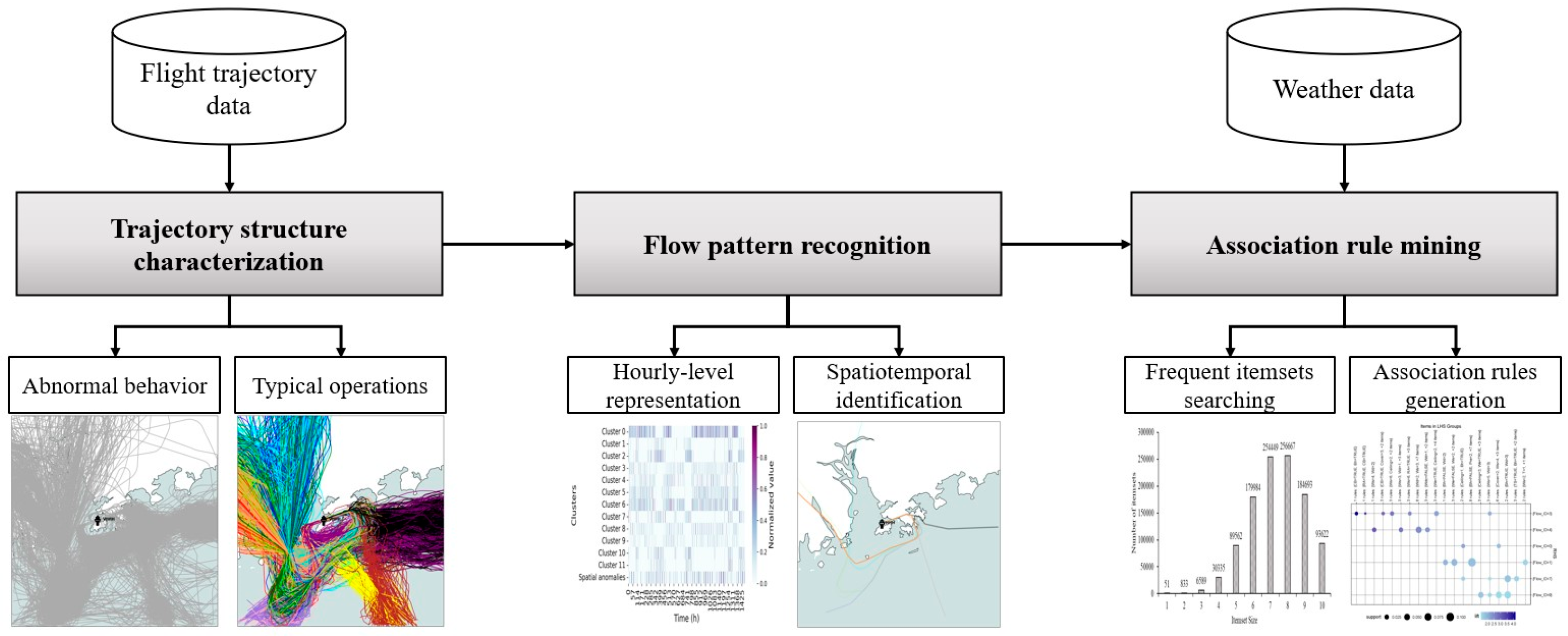
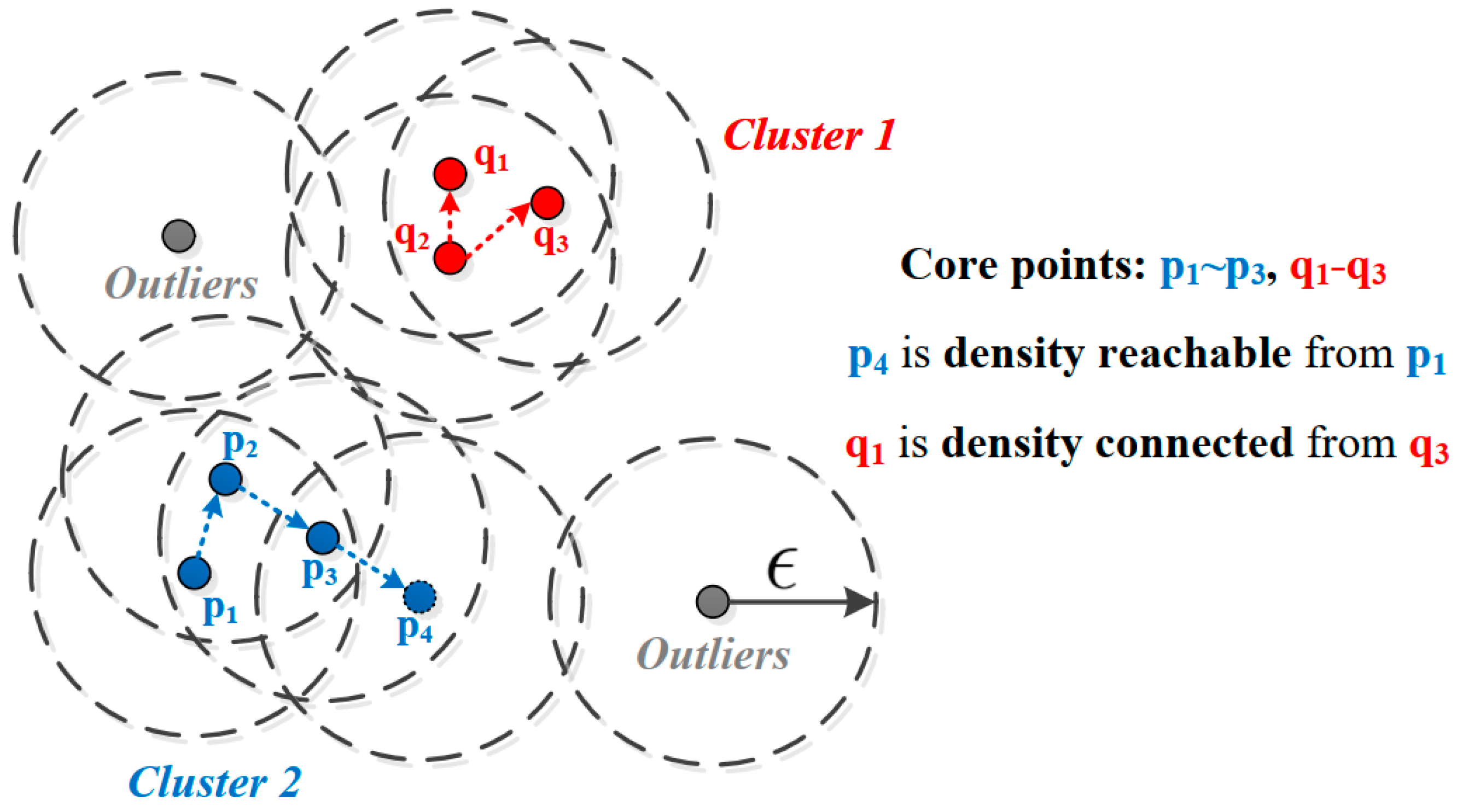
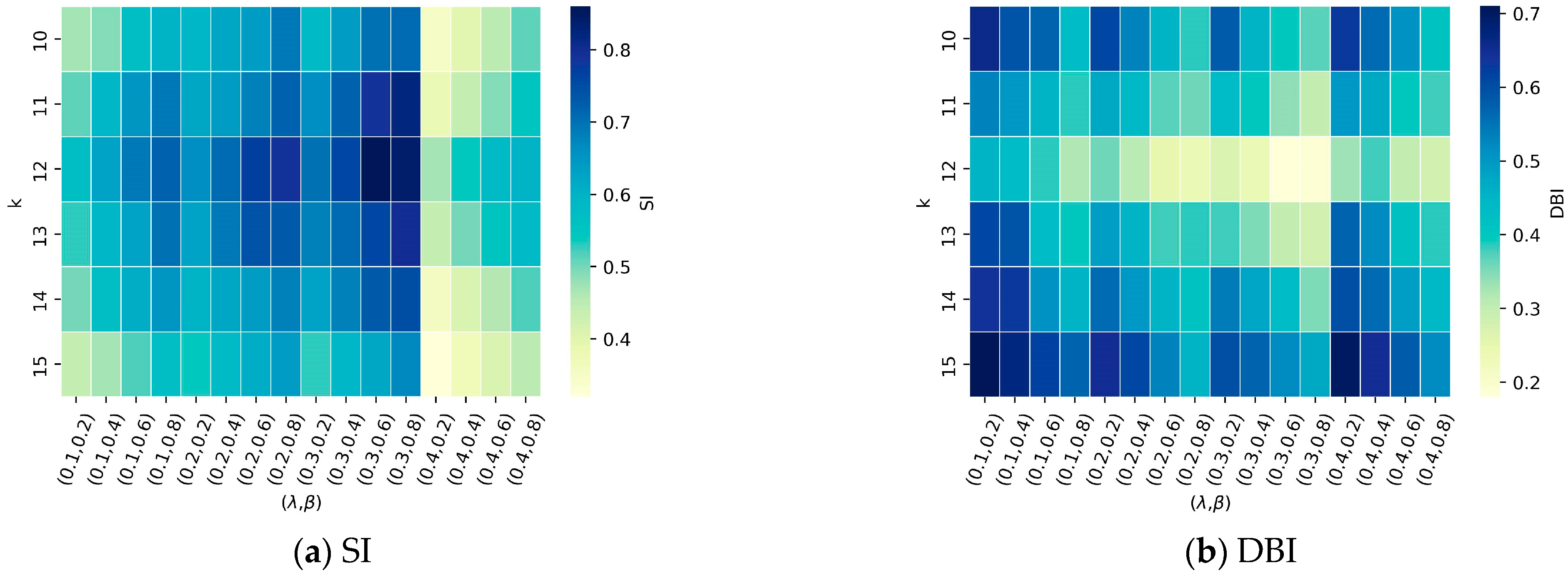
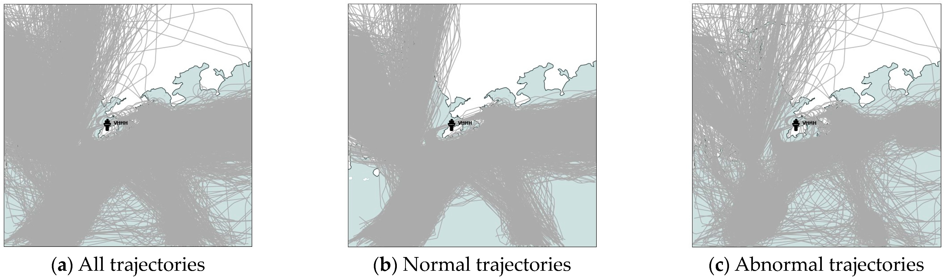
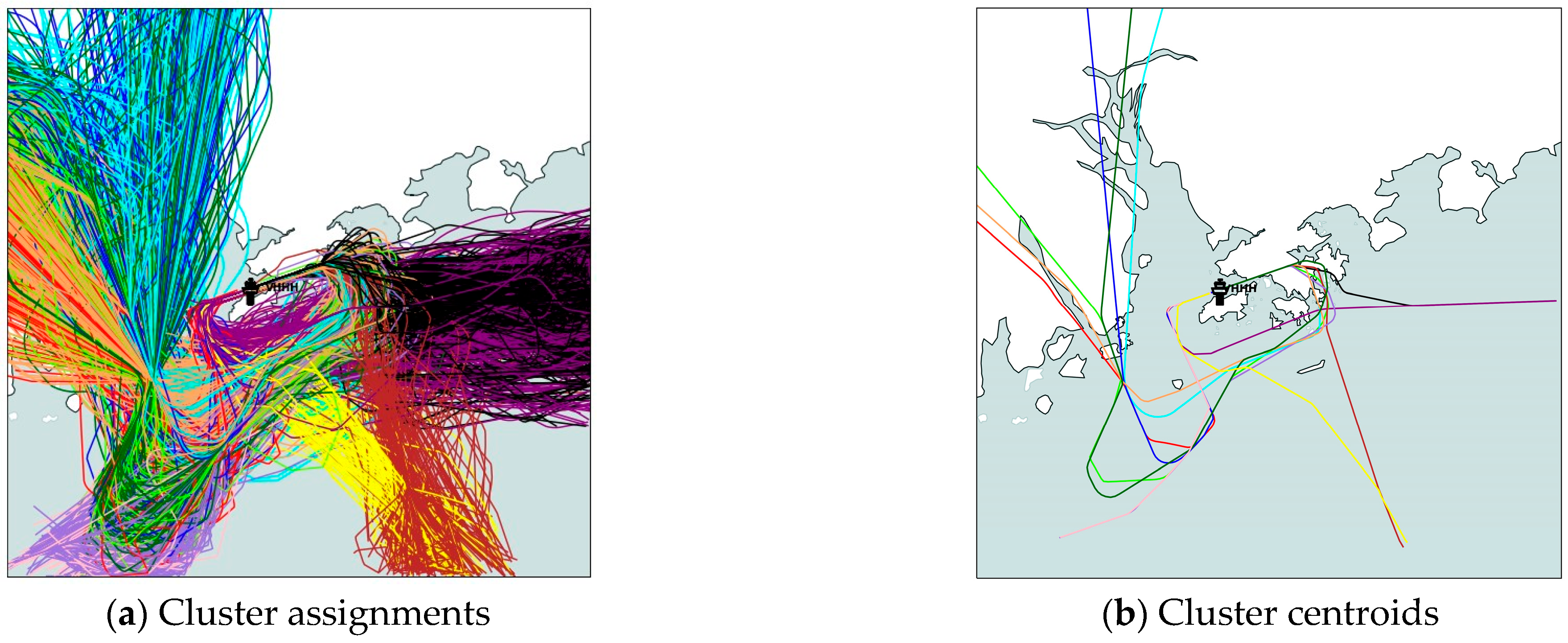

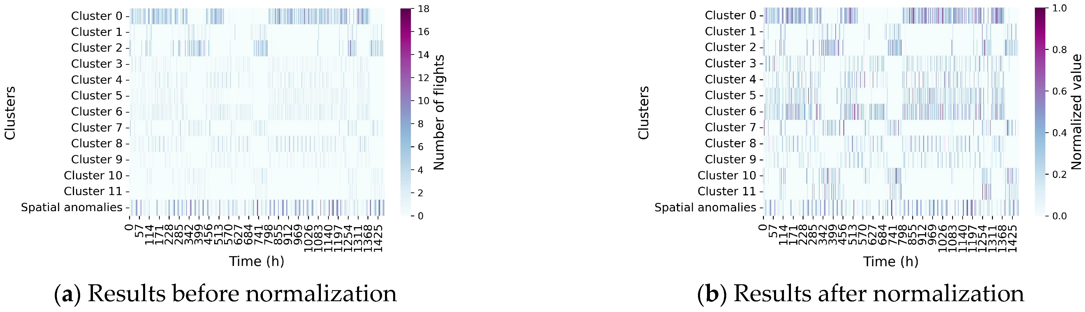

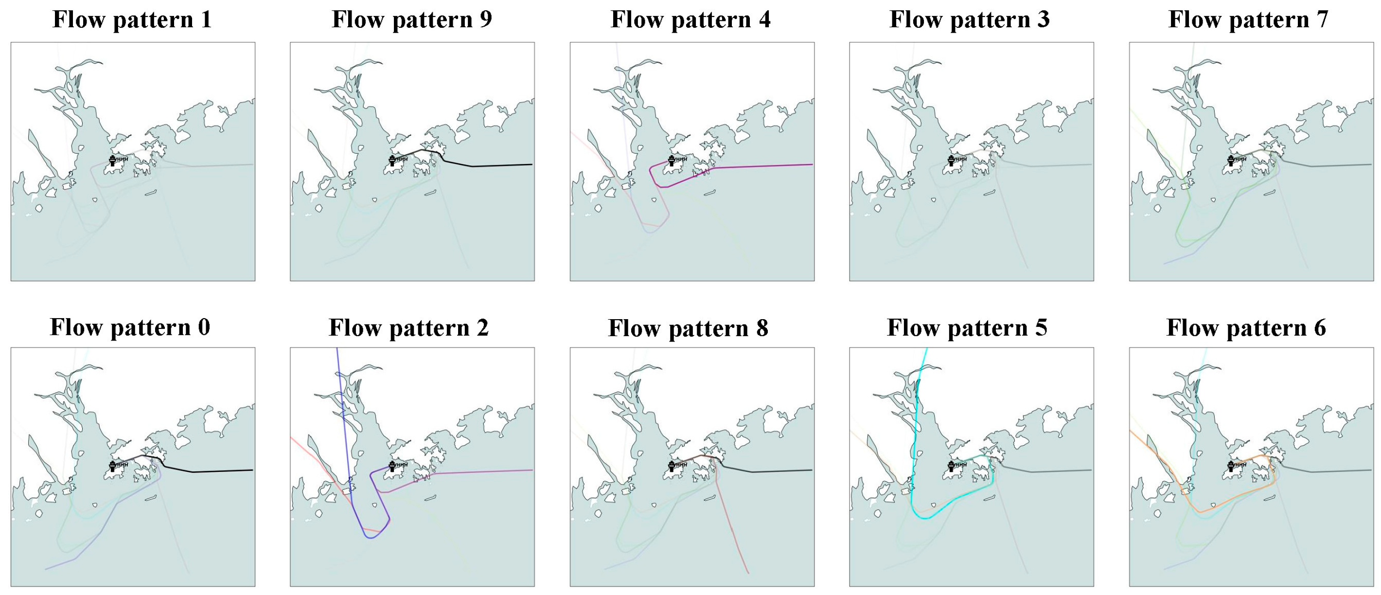

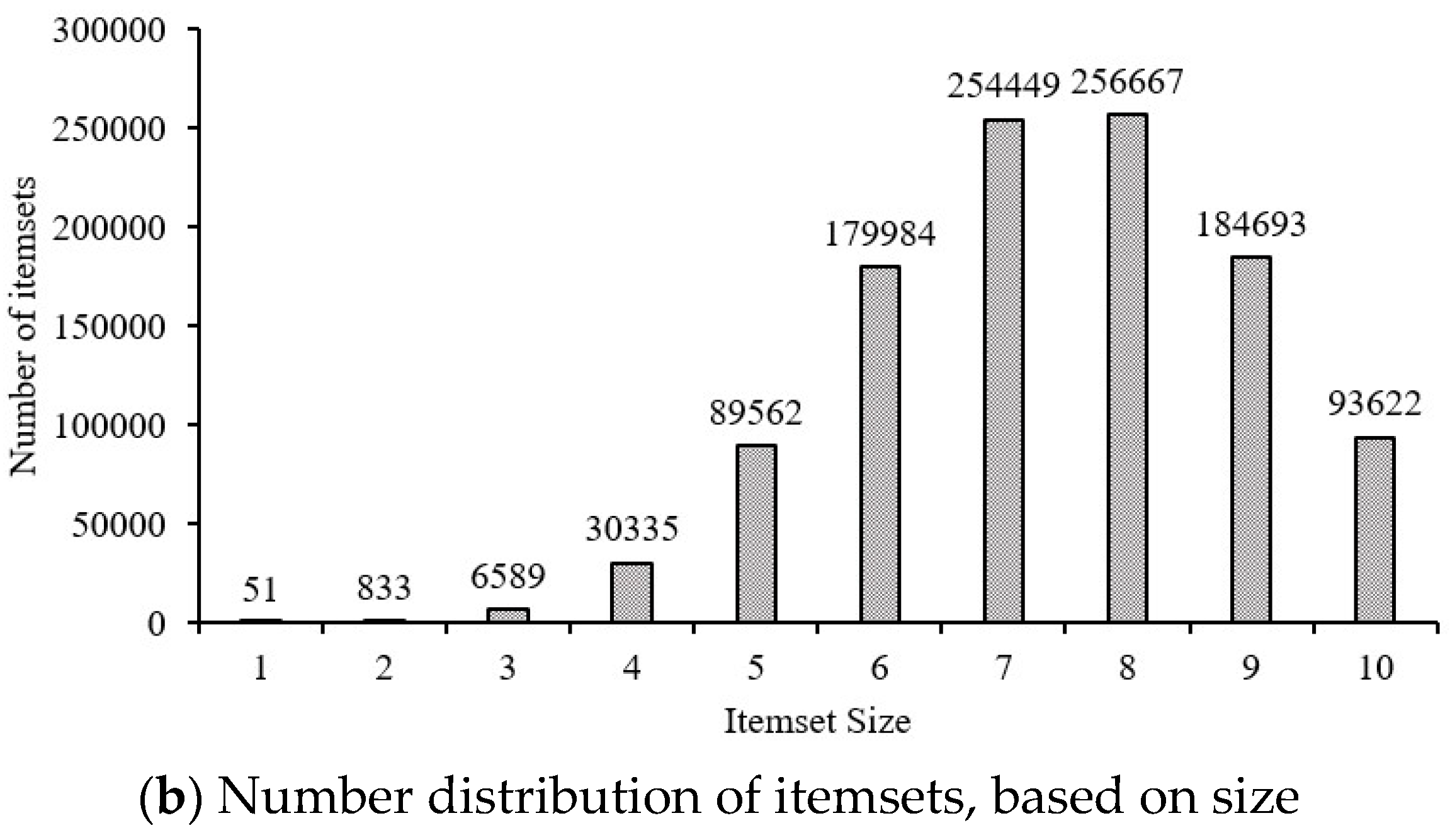
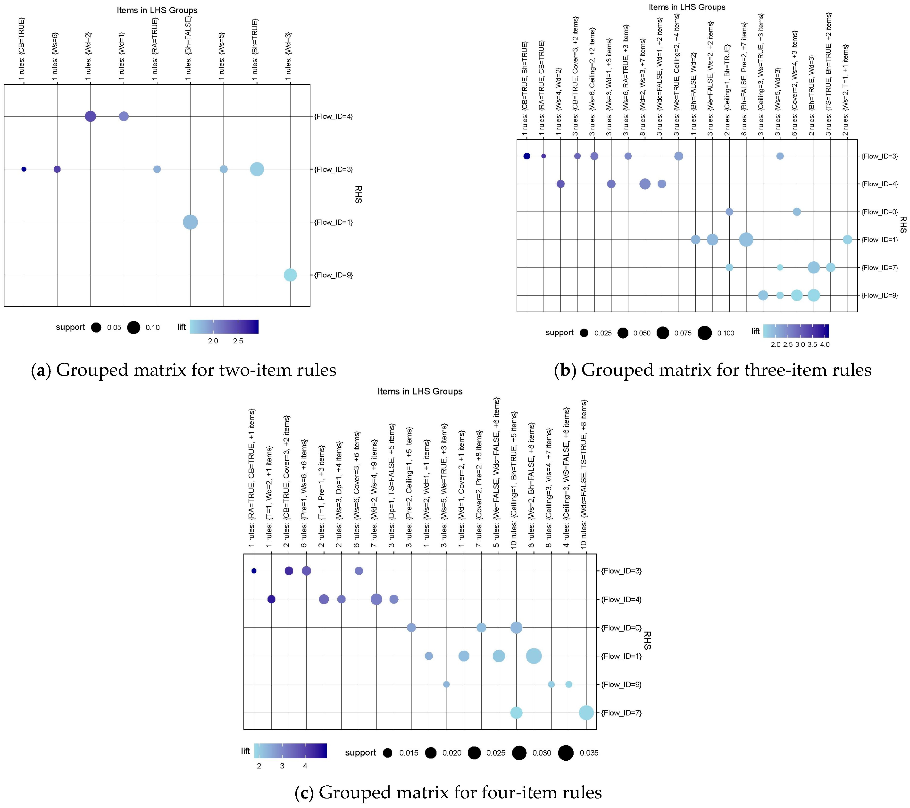
Disclaimer/Publisher’s Note: The statements, opinions and data contained in all publications are solely those of the individual author(s) and contributor(s) and not of MDPI and/or the editor(s). MDPI and/or the editor(s) disclaim responsibility for any injury to people or property resulting from any ideas, methods, instructions or products referred to in the content. |
© 2024 by the authors. Licensee MDPI, Basel, Switzerland. This article is an open access article distributed under the terms and conditions of the Creative Commons Attribution (CC BY) license (https://creativecommons.org/licenses/by/4.0/).