
A Time Series Prediction-Based Method for Rotating Machinery Detection and Severity Assessment


Abstract
1. Introduction
2. Theoretical Fundamental
2.1. Feature Extraction
2.2. Dynamic Time Warping
2.3. Long Short-Term Memory
2.4. Modified Z-Score
3. Proposed Method
4. Experiment Validation
4.1. Case Western Reserve University Bearing Data (CWRU)
4.1.1. Description
4.1.2. Result
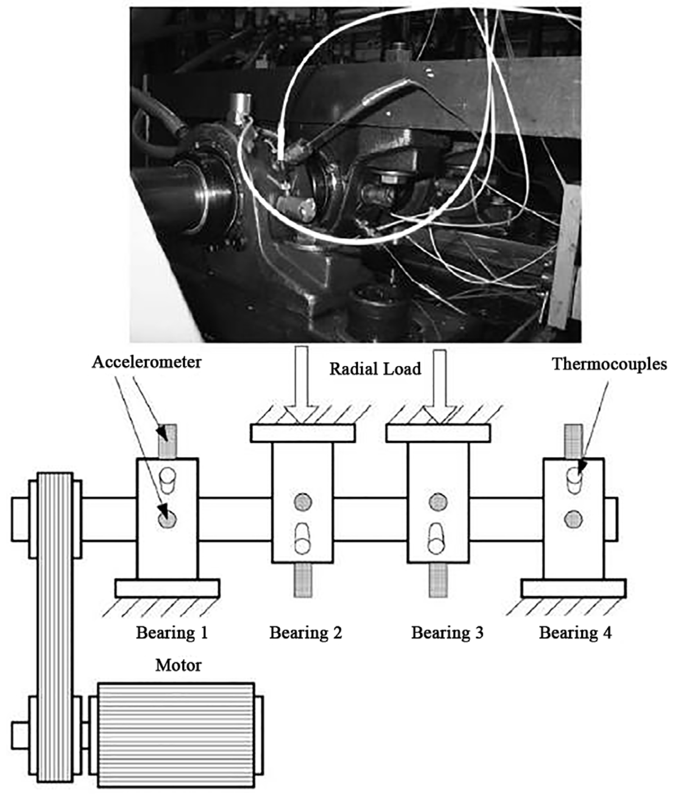
4.2. Dataset of Intelligent Maintenance Systems (IMS), University of Cincinnati
4.2.1. Description
- 4 double-row bearings;
- 2000 rpm stationary speed;
- 6000 lbs load applied onto the shaft and bearing by a spring mechanism;
- high-sensitivity Quart ICP accelerometers.
4.2.2. Results
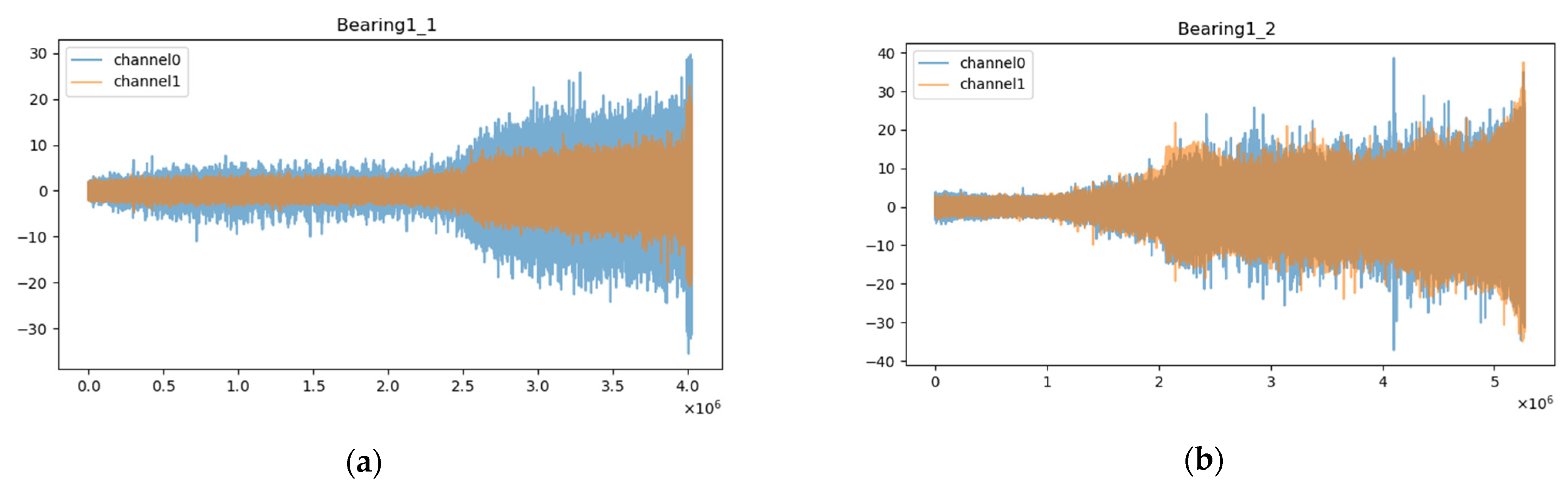
4.3. Xi’an Jiaotong University Bearing Fault Dataset (XJTU-SY)
4.3.1. Description
4.3.2. Results
4.4. Results Analysis
- (1)
- Experiments on the CWRU dataset show that the method can perform fault detection tasks with a small number of samples. Although it uses only 0.021 inch diameter defect data for training, it can detect 0.007 and 0.014 inch diameter defects. This feature is particularly suited to real-world industrial environments. In many practical application scenarios, the acquisition of a large amount of labeled data is often costly and time-consuming. Therefore, an algorithm that can effectively use a limited number of samples for accurate detection is of significant practical value. In addition, this method is versatile and can detect a variety of defects, including inner ring defects, outer ring defects, and rolling element defects, all using the same approach.
- (2)
- Experiments on the IMS dataset demonstrate that this method can be used to monitor the health of rotating machinery and provide timely warnings when the machine exhibits abnormalities. Compared to existing work, our method does not use complex signal analysis techniques, nor does it require manual identification of characteristic lines in spectrograms, yet it detects faults at times similar to or earlier than existing methods. This suggests that the method is more suitable for unsupervised scenarios.
- (3)
- The experiments conducted on the XJTU-SY dataset confirm the conclusions of the previous two experiments. In experiments (1) and (2) on the XJTU-SY dataset, the data used for testing and the data used for feature selection were not the same, which once again demonstrates that this method can perform defect detection tasks with a small number of samples. Furthermore, despite the different operating conditions in (1) and (2), the method proposed in this paper was able to detect the occurrence of faults, demonstrating its universality. Experiment three (3) shows that this method remains effective even when the fault mode of the unknown signal is a mixture of several faults.
5. Conclusions
- (1)
- Overcoming the limitations of traditional strategies that categorize fault severity in a discrete manner, this method uses a continuous indicator to indicate fault severity. As a result, it provides greater flexibility in setting thresholds to differentiate defects.
- (2)
- Thanks to a well-structured algorithmic framework, this method is highly scalable and adaptable. In the feature selection phase, in addition to the 18 features preset in this paper, other new features can be included. In addition to the DTW algorithm used in this paper, other similarity measurement algorithms can be used. During the training phase, other time series prediction models can be used instead of the LSTM network used in this paper. Furthermore, algorithms other than Z-score can be used for outlier detection.
- (3)
- Only a small amount of fault data were used during training (particularly in the feature selection process), yet the method can still effectively detect faults in unknown signals. Given that fault data collection in real-world engineering environments can be challenging, and typically only a small amount of fault data can be obtained, this method is expected to perform well in real-world production scenarios with limited samples.
- (1)
- Training the deep learning model requires a large number of feature time series samples, and obtaining these feature samples requires slicing of the original signals. Therefore, implementing this method requires a sufficient amount of original data, and it may consume significant memory resources during computation.
- (2)
- Manual feature selection is an insufficient approach for many applications. If features could be extracted adaptively using neural network methods, it would save time and resources while increasing generality.
- (3)
- The process of feature selection and thresholding lacks standardized criteria and relies on the subjective decisions of researchers. There is a need for more general and robust methods for adaptive decision-making.
Author Contributions
Funding
Data Availability Statement
Conflicts of Interest
References
- Glowacz, A. Fault diagnosis of single-phase induction motor based on acoustic signals. Mech. Syst. Signal Process. 2019, 117, 65–80. [Google Scholar] [CrossRef]
- Królczyk, G.; Królczyk, J.; Legutko, S.; Hunjet, A. Effect of the Disc Processing Technology on the Vibration Level of the Chipper during Operations. Tehnicki Vjesnik-Technical Gazette. April 2014. Available online: https://www.semanticscholar.org/paper/Effect-of-the-disc-processing-technology-on-the-of-Kr%C3%B3lczyk-Kr%C3%B3lczyk/bb3100ef1c5c6d4ddc99f5927f399de1b5f65c0e (accessed on 16 June 2024).
- Montalvo, C.; Gavilán-Moreno, C.; García-Berrocal, A. Cofrentes nuclear power plant instability analysis using ensemble empirical mode decomposition (EEMD). Ann. Nucl. Energy 2017, 101, 390–396. [Google Scholar] [CrossRef]
- Li, Z.X.; Jiang, Y.; Hu, C.; Peng, Z. Recent progress on decoupling diagnosis of hybrid failures in gear transmission systems using vibration sensor signal: A review. Measurement 2016, 90, 4–19. [Google Scholar] [CrossRef]
- Cerrada, M.; Sánchez, R.-V.; Li, C.; Pacheco, F.; Cabrera, D.; de Oliveira, J.V.; Vásquez, R.E. A review on data-driven fault severity assessment in rolling bearings. Mech. Syst. Signal Process. 2018, 99, 169–196. [Google Scholar] [CrossRef]
- Bujoreanu, C.; Monoranu, R.; Olaru, N.D. Study on the Defects Size of Ball Bearings Elements Using Vibration Analysis. Appl. Mech. Mater. 2014, 658, 289–294. [Google Scholar] [CrossRef]
- Singh, M.; Kumar, R. Thrust bearing groove race defect measurement by wavelet decomposition of pre-processed vibration signal. Measurement 2013, 46, 3508–3515. [Google Scholar] [CrossRef]
- Zhao, S.; Liang, L.; Xu, G.; Wang, J.; Zhang, W. Quantitative diagnosis of a spall-like fault of a rolling element bearing by empirical mode decomposition and the approximate entropy method. Mech. Syst. Signal Process. 2013, 40, 154–177. [Google Scholar] [CrossRef]
- Pan, H.; He, X.; Tang, S.; Meng, F. An Improved Bearing Fault Diagnosis Method using One-Dimensional CNN and LSTM. Stroj. Vestn.—J. Mech. Eng. 2018, 64, 443–452. [Google Scholar] [CrossRef]
- Guo, X.; Shen, C.; Chen, L. Deep Fault Recognizer: An Integrated Model to Denoise and Extract Features for Fault Diagnosis in Rotating Machinery. Appl. Sci. 2017, 7, 41. [Google Scholar] [CrossRef]
- Shao, H.; Jiang, H.; Lin, Y.; Li, X. A novel method for intelligent fault diagnosis of rolling bearings using ensemble deep auto-encoders. Mech. Syst. Signal Process. 2018, 102, 278–297. [Google Scholar] [CrossRef]
- Shen, C.; Hu, F.; Liu, F.; Zhang, A.; Kong, F. Quantitative recognition of rolling element bearing fault through an intelligent model based on support vector regression. In Proceedings of the 2013 Fourth International Conference on Intelligent Control and Information Processing (ICICIP), Beijing, China, 9–11 June 2013; IEEE: Piscataway, NJ, USA, 2013; pp. 842–847. [Google Scholar] [CrossRef]
- Lei, Y.; He, Z.; Zi, Y. EEMD method and WNN for fault diagnosis of locomotive roller bearings. Expert Syst. Appl. 2011, 38, 7334–7341. [Google Scholar] [CrossRef]
- Smith, A.J.; Powell, K.M. Fault Detection on Big Data: A Novel Algorithm for Clustering Big Data to Detect and Diagnose Faults. IFAC-PapersOnLine 2019, 52, 328–333. [Google Scholar] [CrossRef]
- Chang, Y.-J.; Hsu, H.-K.; Hsu, T.-H.; Chen, T.-T.; Hwang, P.-W. The Optimization of a Model for Predicting the Remaining Useful Life and Fault Diagnosis of Landing Gear. Aerospace 2023, 10, 963. [Google Scholar] [CrossRef]
- Rauber, T.W.; Boldt, F.d.A.; Varejao, F.M. Heterogeneous Feature Models and Feature Selection Applied to Bearing Fault Diagnosis. IEEE Trans. Ind. Electron. 2015, 62, 637–646. [Google Scholar] [CrossRef]
- Keogh, E.; Ratanamahatana, C.A. Exact indexing of dynamic time warping. Knowl. Inf. Syst. 2005, 7, 358–386. [Google Scholar] [CrossRef]
- Wang, G.; Wang, T.; Chen, J.; Zhao, S. Bearing fault feature selection method based on dynamic time warped related searches. J. Vibroeng. 2023, 25, 311–324. [Google Scholar] [CrossRef]
- Chen, J.; Wang, D. Long short-term memory for speaker generalization in supervised speech separation. J. Acoust. Soc. Am. 2017, 141, 4705–4714. [Google Scholar] [CrossRef] [PubMed]
- Hochreiter, S.; Schmidhuber, J. Long short-term memory. Neural Comput. 1997, 9, 1735–1780. [Google Scholar] [CrossRef] [PubMed]
- Sabir, R.; Rosato, D.; Hartmann, S.; Guehmann, C. LSTM Based Bearing Fault Diagnosis of Electrical Machines using Motor Current Signal. In Proceedings of the 2019 18th IEEE International Conference on Machine Learning And Applications (ICMLA), Boca Raton, FL, USA, 16–19 December 2019; IEEE: Piscataway, NJ, USA, 2019; pp. 613–618. [Google Scholar] [CrossRef]
- Kaliyaperumal, S.M.K.; Arumugam, S. Labeling Methods for Identifying Outliers. Int. J. Stat. Syst. 2015, 10, 231–238. [Google Scholar]
- Welcome to the Case Western Reserve University Bearing Data Center Website|Case School of Engineering|Case Western Reserve University. Case School of Engineering. Available online: https://engineering.case.edu/bearingdatacenter/welcome (accessed on 12 March 2024).
- NASA Bearing Dataset. Available online: https://www.kaggle.com/datasets/vinayak123tyagi/bearing-dataset (accessed on 12 March 2024).
- Lei, Y.; Han, T.; Wang, B.; Li, N.; Yan, T.; Yang, J. XJTU-SY Rolling Element Bearing Accelerated Life Test Datasets: A Tutorial. J. Mech. Eng. 2019, 55, 1. [Google Scholar] [CrossRef]
- Gousseau, W.; Antoni, J.; Girardin, F.; Griffaton, J. Analysis of the Rolling Element Bearing Data Set of the Center for Intelligent Maintenance Systems of the University of Cincinnati. CM2016, Charenton, France. October 2016. Available online: https://hal.science/hal-01715193 (accessed on 11 May 2024).
- Wang, B.; Lei, Y.; Li, N.; Li, N. A Hybrid Prognostics Approach for Estimating Remaining Useful Life of Rolling Element Bearings. IEEE Trans. Reliab. 2020, 69, 401–412. [Google Scholar] [CrossRef]
- Sacerdoti, D.; Strozzi, M.; Secchi, C. A Comparison of Signal Analysis Techniques for the Diagnostics of the IMS Rolling Element Bearing Dataset. Appl. Sci. 2023, 13, 5977. [Google Scholar] [CrossRef]


| Feature | Definition | Domain | Feature | Definition | Domain |
|---|---|---|---|---|---|
| RMS | Time | CF | Time | ||
| SRA | Time | IF | Time | ||
| KV | Time | MF | Time | ||
| SV | Time | SF | Time | ||
| PPV | Time | KF | Time | ||
| FC | Frequency | RVF | Frequency | ||
| RMSF | Frequency | Mean | Statistical | ||
| Var | Statistical | Std | Statistical | ||
| Max | Statistical | Min | Statistical |
| Fault Diameter | Inner Race | Ball | Outer Race (Position 6:00) | Outer Race (Position 9:00) | Outer Race (Position 12:00) |
|---|---|---|---|---|---|
| 0.007″ | 109 | 122 | 135 | 148 | 161 |
| 0.014″ | * | 189 | 201 | * | * |
| 0.021″ | 213 | 226 | 238 | 250 | 262 |
| Parameter | Value | Parameter | Value |
|---|---|---|---|
| L | 2048 | m | 100 |
| piece | 22,000 | p | 10 |
| fL | 110 | fpiece | 200 |
| Feature | DTW Score | Feature | DTW Score |
|---|---|---|---|
| Mean | 29.77 | Var | 17.63 |
| RVF | 19.87 | KF | 17.51 |
| RMSF | 19.70 | Min | 17.31 |
| SRA | 18.11 | FC | 17.09 |
| RMS | 17.85 | MF | 16.99 |
| Fault Type | Inner Race | Outer Race (Position 6:00) | Outer Race (Position 9:00) | Outer Race (Position 12:00) |
|---|---|---|---|---|
| Reference fault signal | 213 | 238 | 250 | 262 |
| Best feature | KV | Min | Mean | Mean |
| DTW score of the best feature | 17.67 | 18.50 | 17.07 | 16.11 |
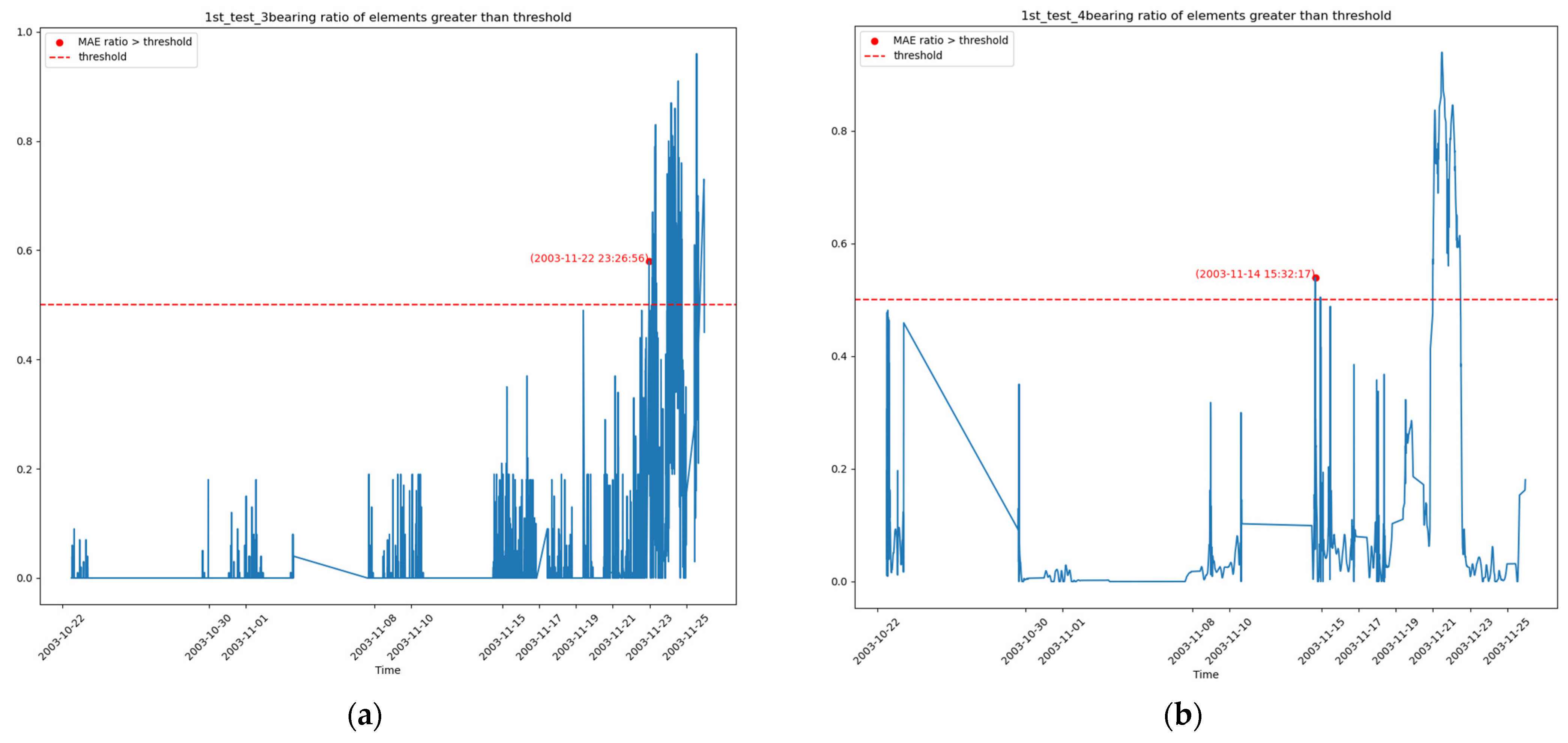
| Study | Bearing 3 | Bearing 4 |
|---|---|---|
| [25] | Time–frequency analysis: 33.8 days (11/23) Envelope spectrum analysis: 32 days (11/22) Spectral coherence analysis: 29.2 days (11/19) | Time–frequency analysis: 18 days (11/8) Envelope spectrum analysis: 25 days (11/15) Spectral coherence analysis: 23 days (11/13) |
| [26] | Last part of the 33rd day (11/23) and the 34th day (11/24) | From the 26th (11/16) day until the end |
| Parameter | Value | Parameter | Value |
|---|---|---|---|
| Inner race diameter (mm) | 29.30 | Ball diameter (mm) | 7.92 |
| Outer race diameter (mm) | 39.80 | Number of balls | 8 |
| Bearing median diameter (mm) | 34.55 | Contact angle (°) | 0 |
| Basic rated dynamic load (N) | 12,820 | Basic rated static load (N) | 6.65 |
| Number | 1 | 2 | 3 |
|---|---|---|---|
| Rotational Speed | 2100 | 2250 | 2400 |
| Radial Force | 12 | 11 | 10 |
Disclaimer/Publisher’s Note: The statements, opinions and data contained in all publications are solely those of the individual author(s) and contributor(s) and not of MDPI and/or the editor(s). MDPI and/or the editor(s) disclaim responsibility for any injury to people or property resulting from any ideas, methods, instructions or products referred to in the content. |
© 2024 by the authors. Licensee MDPI, Basel, Switzerland. This article is an open access article distributed under the terms and conditions of the Creative Commons Attribution (CC BY) license (https://creativecommons.org/licenses/by/4.0/).
Share and Cite
Zhang, W.; Sun, Z.; Lv, D.; Zuo, Y.; Wang, H.; Zhang, R. A Time Series Prediction-Based Method for Rotating Machinery Detection and Severity Assessment. Aerospace 2024, 11, 537. https://doi.org/10.3390/aerospace11070537
Zhang W, Sun Z, Lv D, Zuo Y, Wang H, Zhang R. A Time Series Prediction-Based Method for Rotating Machinery Detection and Severity Assessment. Aerospace. 2024; 11(7):537. https://doi.org/10.3390/aerospace11070537
Chicago/Turabian StyleZhang, Weirui, Zeru Sun, Dongxu Lv, Yanfei Zuo, Haihui Wang, and Rui Zhang. 2024. "A Time Series Prediction-Based Method for Rotating Machinery Detection and Severity Assessment" Aerospace 11, no. 7: 537. https://doi.org/10.3390/aerospace11070537
APA StyleZhang, W., Sun, Z., Lv, D., Zuo, Y., Wang, H., & Zhang, R. (2024). A Time Series Prediction-Based Method for Rotating Machinery Detection and Severity Assessment. Aerospace, 11(7), 537. https://doi.org/10.3390/aerospace11070537