Accurate Method for Estimating Wall-Friction Based on Analytical Wall-Law Model

Abstract

A novel method is proposed for accurately determining the local wall friction through the near-wall measurement of time-average velocity profile in a Type-A turbulent boundary layer (TBL). The method is based on the newly established analytical wall-law in Type-A TBL. The direct numerical simulations (DNS) data of turbulence on a zero-pressure-gradient flat-plate (ZPGFP) is used to demonstrate the accuracy and the robustness of the approach. To verify the reliability and applicability of the method, a two-dimensional particle image velocimetry (PIV) measurement was performed in a ZPGFP TBL with a low-to-moderate Reynolds number (Re). Via utilizing the algorithm of single-pixel ensemble correlation (SPEC), the velocity profiles in the ZPGFP TBL were resolved at a significantly improved spatial resolution, which greatly enhanced the measurement accuracy and permitted us to accurately capture the near-wall velocity information. The accuracy of the approach is then quantitatively validated for the high Reynolds number turbulence using the ZPGFP TBL data. The research demonstrates that the current method can provide the precise estimation of wall friction with a mean error of less than 2%, which not only possesses the advantage of its insensitivity to the absolute wall-normal distance of the measuring point, but also its capability of providing an accurate prediction of wall shear stress based on fairly sparse experimental data on the velocity profile. The current study demonstrates that the wall shear stress can be accurately estimated by a velocity even at a single-point either measured or calculated in the near-wall region.

1. Introduction

The wall-bounded turbulences are quite common in current industrial applications with the determination of wall shear stress (WSS) being one of the challenging issues vital for engineers to help understand the fluid–wall interactions and to design the related mechanics. Therefore, the fluid physics and mechanics communities have conducted a long history of research focusing on measuring and calculating the turbulence WSS from the closely related velocity profiles. Within this context, searching for the turbulence friction wall-laws has been one of the well-known efforts ever since Prandtl [1] developed the turbulent boundary layer (TBL) theory and von Kármán [2] established the law-of-the-wall for the TBL on a zero-pressure-gradient flat-plate (ZPGFP). From then on, the numerous studies on TBL wall-laws, such as the works in [3,4,5,6], have provided profound understandings on the Reynolds number (Re) independent relations between the WSS and the velocity profiles, the TBL velocity similarity and even the extension of the law model to the temperature field in thermal turbulence [7]. These fundamental research works firmly demonstrate and prove that the accurate and detailed knowledges on WSS are important for characterizing a wall-bounded turbulence. Accurate measurement of WSS is not only important for turbulence theory study but also crucial for numerical simulations, including RANS and LES [8,9]. It is vital for successfully exploring more precise wall-law relations based on the ever-expanding experimental and computational data, mainly from Direct Numerical Simulation (DNS), of complex-geometry wall turbulence.

On the fluid experiment side, the traditional indirect pressure-based methods, such as the Preston tube [10], relies heavily on the traditional law-of-the-wall and suffers from the limitations arising from its intrusive nature. The floating-element force-balance method can be directly applied to measures the skin friction. However, the measurements are affected, to a large extend, by the alignment accuracies between the floating-element surface and the tested wall. With the developments in microelectromechanical system (MEMS), several methods arose based on the technology progress [11,12], such as MEMS-based hot-wire (HW), MEMS-based hot-film and MEMS-based floating element. A comprehensive review can be found in Naughton et al. [13] for the available WSS measurement techniques. The other WSS measuring technologies include the thin-oil-film interferometric method [14] and the oil-droplet interferometric method [15], which has become quite common in the fluid research laboratories and to some extent in engineering practices over the past thirty years. These methods are based on the relationship between thickness of an oil-film, or an oil-droplet deposited onto the testing surface exposed to the local shear stress due to the flow.

An alternative approach was to make use of the achievement of the wall-law models to estimate the WSS based on the measured near-wall mean velocity profile [16,17], including the linear law in the viscous sublayer and the logarithmic-linear law (or log-law) in the semi-log sublayer. For instance, the Clauser chart method [18,19] was used to estimate the WSS based the log-law within the semi-log sublayer, However, the applicability of the approach was limited by the fact that it required the knowledge of the sublayer’s applicable range and the associated constants beforehand. Albeit the existence of log-law is quite well-accepted by the fluid mechanics community, the constants in the log-law along with their applicable range and precision are yet to be determined and are quite debatable [20,21]. Marusic et al. [20] suggested that although the log-law formulation was a preferred description for the mean velocity profile in a wall turbulence, the universality of its parameters and the extent of the logarithmic overlap region had been a subject of debate. Even nowadays, it is still an open question whether the lower limit of the log-law is a function of Reynolds number and whether the discrepancies between the log-law and the experimental data can be attributed to an inadequate probe size or other ambiguities in the interpretation of data. The log-law constants number also appears to be dependent on the flow configuration [22]. For example, the constants appears to be $\kappa =0.42$ and $B=5.6$ in a pipe turbulence, $\kappa =0.41$ and $B=5.1$ in the TBL of ZPGFP, and for a channel TBL, $\kappa$ = 0.36–0.39 which is clearly less than the most widely used value of $\kappa =0.41$.

Additionally, the van Driest and Spalding models were attempted by McEligot [23] and Kendall [24], respectively, for a better prediction of WSS. These methods are based on log-law model, which only address the issue of prediction accuracy being affected by the lower bound of the data interval. Moreover, Djenidi [25] used the wake law to predict WSS, which has a broad range of data points. However, the accuracy of this method is largely limited by the precision of the nominal boundary layer thickness.

Another way to estimate the WSS is referred to as the wall-slope method within the viscous sublayer satisfying the linear-law relation of $u^{+}=y^{+},y^{+}\le 5.0$, which requires no other assumption except the constant velocity gradient [26] and a simple least-squares fitting technique can thus be applied to determine the WSS by ${\tau }_w=\mu du/dy$. In this regard, Wang et al. [26] and Shen et al. [27] measured the WSS using the wall-slope method combined with a high-resolution particle image velocimetry (PIV) in water channel at the low-to-moderate Reynolds number. However, due to the fact that the viscous sublayer is very thin in terms of its dimension perpendicular to wall (around a hundred-micron in scale), an extremely high spatial resolution is required for the velocity measurement. The requirement becomes impractically difficult and expensive when measuring the velocity at a high Reynolds number. To improve the number of velocity points being included in the fitting technique, an extend method is suggested by Örlü [28] using an additional fourth- and fifth-order of polynomial terms. Another method based on momentum equation and Taylor series expansion was proposed by Durst [29] to enlarge the applicable range of linear law, which needs to introduce a total of four or five parameters to be estimated in the measurement.

Based on the above literature reviews, it is evident that the accuracy of WSS measurement is greatly impacted by the precisions of experimental means, such as the HW, hot-film and floating element, which has been significantly improved by the MEMS-based technologies. Meanwhile, the progress of WSS measuring technology heavily relies on the wall-law models which is predominantly founded on the traditional law-of-the-wall given by von Kármán [2] under the framework of TBL theory [1], including the viscous sublayer model of linear law and the semi-log sublayer model of linear log-law. From the authors’ point of view, in order to improve the accuracy of the traditional wall-law model, two key issues have to be addressed and resolved so that more accurate law formulations can be developed, which include (1) the TBL sublayers have to be quantitatively well-defined and (2) the analytical wall-law models have to be constructed for the sublayers with not only the continuity of analytical function of velocity, but also its derivative particularly at the joint locations of sublayers, since the WSS calculation needs to accurately evaluate the velocity derivative. Within this context, Wang et al. [5] successfully developed a wall-law model satisfying these requirements and strictly validated the model using DNS data. On the other hand, the experimental fluid mechanics has developed the quite matured particle image velocimetry (PIV) [30,31] method, which is nowadays popularly applied as a non-intrusive means to measure the velocity vector in both two-dimensional and three-dimension field.

Within this context, the present study utilizes the high-resolution flow-field post-processing technology (SPEC, Single Pixel Ensemble Correlation) and the PIV measurement to validate the accuracy of analytical wall-law models and moreover to make use of the model to obtain an accurate WSS in Type-A TBL. The robustness of the approach is first verified and demonstrated via the benchmark with the existing DNS data. Following these verifications, a rigorous comparison and validation are conducted between the prediction using the wall-law model and the measured wall friction based on the equilibrium method at the low-to-moderate Reynolds number. Finally, the method is applied to the high Reynolds number and compared with the results of WSS measured using the oil-film method. The development of analytical wall-law models significantly expands the current PIV measurement capability in terms of the obtaining an accurate WSS which represents quite a challenging issue facing the fluid engineering industry.

2. Development of Methodology for Determining WSS

2.1. Comments on the Existing WSS Estimations Based on the Traditional Wall-Law

According to the conventional Law-of-the-Wall, the streamwise velocity component in an incompressible ZPGFP TBL can simply be divided into two layers in the wall-normal direction, namely the inner and outer layers. The inner layer is usually defined in the region of $0.0<y/\delta <0.1$ with $\delta$ being the nominal thickness of TBL (99% of the streamwise velocity component outside TBL). The inner layer can be further subdivided into three sublayers and is usually described by:

• the viscous sublayer

  $$u^{+}=y^{+},y^{+}\le 5.0;$$

  (1)
• the logarithmic sublayer

  $$u^{+}=\frac{1}{\kappa }ln{y}^{+}+B,y^{+}>30.0;$$

  (2)
• the buffer layer, interval between the viscous and logarithmic sublayers, $5.0\le y^{+}\le 30.0$, where $u^{+}$ and $y^{+}$ are defined as $u^{+}=u/u_{\tau }$ and $y^{+}=y{u}_{\tau }/\nu$, respectively, with $u_{\tau }$ representing the local friction velocity, and these definitions are essentially consistent with the traditional law-of-the-wall.

Equation (1) is the linear law characterized by the constant velocity gradient. In the linear-law sublayer, the molecular viscous stress dominates and are much larger than the turbulent or Reynolds stress. Equation (2) represents the logarithmic law, or log law, formulated by von Kármán with the $\kappa$ being well-known as the von Kármán constant and B being the constant standing for the effects of surface roughness. In the existing literatures as mentioned earlier, the two log-law constants are found not a quite universal or fixed constant depending on the flow configurations and Reynolds numbers. However, the most commonly accepted empirical values for the constants are $\kappa =0.41$ and $B=5.1$. Based on Equations (1) and (2), the WSS can thus be estimated by the experimental data in a dimensional form, which is known as the wall-slope method and the Clauser chart method mentioned above. However, both the methods are suffered, respectively, by their own severe technology hampers when measuring the turbulent velocity data required for WSS calculation in an experiment.

The wall-slope method demands an accurate velocity measurement in the very near-wall region as required by the traditional wall-law in Equation (1), i.e., $y^{+}<5.0$, which poses an almost insurmountable difficulty for the velocity measuring devices due to the extremely high spatial resolution requirement in a high-Re TBL experiment. On the other hand, the Clauser chart method is facing the uncertainties in the wall-law model caused by the drifting values of the constants ($\kappa ,B$) associated with the different TBL configurations and Re numbers. Therefore, these technology bottlenecks are evidently caused by the lack of a sufficient accurate wall-law model, which calls for a new wall-law formulation with more precision to surpass the traditional model.

2.2. Recent Development of the More Advanced Analytical Wall-Law Model

Thanks to the rapid progress of direct numerical simulation (DNS) of turbulence and the consequent availability of fast-growing DNS databases, the more accurate wall-law models with a system of analytical formulations were established by Wang and Xu for the Type-A TBL in [5] including a ZPGFP TBL and for the Type-B TBL in [7] even applicable to the thermal turbulence with a temperature field. Comparing to the traditional model, the novel wall laws were obtained with the triple-control-parameters for entire Type-A TBL, including both u and v components of mean velocity. The highlights of the law development are summarized as following:

(1) The generic TBL [1] were appropriately classified into the three types based on their universal governing equations, namely Type-A, -B and -C TBL, based on the time-averaged WSS distribution patterns as given by: Type-A of ${\tau }_w={\tau }_w\left(x\right)$, Type-B of ${\tau }_w={\tau }_w\left(z\right)$ or ${\tau }_w={\tau }_w\left(y\right)$ and Type-C of ${\tau }_w={\tau }_w(x,z)$ or ${\tau }_w={\tau }_w(x,y)$ with ${\tau }_w$ being the local WSS, x being the streamwise and y or z being the wall-normal or spanwise directions, respectively. Thereby, the two important TBL scales were identified, namely the time-averaged local frictional scales $\left({\tau }_w\right)$ popularly used in the traditional wall-law studies and the ensemble-averaged frictional scales $\left(\overline{{\tau }_w}\right)$ [5] successfully applied in the new wall-law development.

Based on the ensemble-averaged wall shear stress $\overline{{\tau }_w}$, the nondimensionalized Navier–Stokes equations can be written in the form of Equations (3)–(6). These equations are Re-independent and therefore, are suitable to be applied to the wall-law study.

$$\frac{\partial u^{*}}{\partial x^{*}}+\frac{\partial v^{*}}{\partial y^{*}}+\frac{\partial w^{*}}{\partial z^{*}}=0$$

(3)

$$\frac{\partial u^{*}}{\partial t^{*}}+\frac{\partial u^{*}{u}^{*}}{\partial x^{*}}+\frac{\partial u^{*}{v}^{*}}{\partial y^{*}}+\frac{\partial u^{*}{w}^{*}}{\partial z^{*}}=-\frac{\partial p^{*}}{\partial x^{*}}+\frac{{\partial }^2{u}^{*}}{\partial {x^{*}}^2}+\frac{{\partial }^2{u}^{*}}{\partial {y^{*}}^2}+\frac{{\partial }^2{u}^{*}}{\partial {z^{*}}^2}$$

(4)

$$\frac{\partial v^{*}}{\partial t^{*}}+\frac{\partial v^{*}{u}^{*}}{\partial x^{*}}+\frac{\partial v^{*}{v}^{*}}{\partial y^{*}}+\frac{\partial v^{*}{w}^{*}}{\partial z^{*}}=-\frac{\partial p^{*}}{\partial y^{*}}+\frac{{\partial }^2{v}^{*}}{\partial {x^{*}}^2}+\frac{{\partial }^2{v}^{*}}{\partial {y^{*}}^2}+\frac{{\partial }^2{v}^{*}}{\partial {z^{*}}^2}$$

(5)

$$\frac{\partial w^{*}}{\partial t^{*}}+\frac{\partial w^{*}{u}^{*}}{\partial x^{*}}+\frac{\partial w^{*}{v}^{*}}{\partial y^{*}}+\frac{\partial w^{*}{w}^{*}}{\partial z^{*}}=-\frac{\partial p^{*}}{\partial z^{*}}+\frac{{\partial }^2{w}^{*}}{\partial {x^{*}}^2}+\frac{{\partial }^2{w}^{*}}{\partial {y^{*}}^2}+\frac{{\partial }^2{w}^{*}}{\partial {z^{*}}^2}$$

(6)

For the Type-A TBL, the time and spatial averaging on Equations (3)–(6) yields Equations (7)–(9), which serves as the foundation for Type -A TBL wall-law development.

$$\frac{\partial \overline{u^{*}}}{\partial x^{*}}+\frac{\partial \overline{v^{*}}}{\partial y^{*}}=0$$

(7)

$$\frac{\partial \overline{u^{*}{u}^{*}}}{\partial x^{*}}+\frac{\partial \overline{u^{*}{v}^{*}}}{\partial y^{*}}=\frac{{\partial }^2\overline{u^{*}}}{\partial x^{*2}}+\frac{{\partial }^2\overline{u^{*}}}{\partial y^{*2}}+\frac{\partial \overline{u^{*\prime }{u}^{*\prime }}}{\partial x^{*}}+\frac{\partial \overline{u^{*\prime }{v}^{*\prime }}}{\partial y^{*}}$$

(8)

$$\frac{\partial \overline{u^{*}}\overline{v^{*}}}{\partial x^{*}}+\frac{\partial \overline{v^{*}}\overline{v^{*}}}{\partial y^{*}}=\frac{{\partial }^2\overline{v^{*}}}{\partial x^{*2}}+\frac{{\partial }^2\overline{v^{*}}}{\partial y^{*2}}+\frac{\partial \overline{u^{*\prime }{v}^{*\prime }}}{\partial x^{*}}+\frac{\partial \overline{v^{*\prime }{v}^{*\prime }}}{\partial y^{*}}$$

(9)

where $\overline{u^{*}}=u/\overline{u_{\tau }}$, $x^{*}=\rho \overline{u_{\tau }}x/\mu$, $y^{*}=\rho \overline{u_{\tau }}y/\mu$ with ($u,v$) being the streamwise and wall-normal velocity components.

(2) The study in [5] found that the three-types of functions with the distinctive triple-control parameters were important and sufficient in universally describing and predicting the TBL velocity profiles for both streamwise (u) and wall-normal (v) components in a semi-infinite flat plate. These functions include: (a) the base function of $f\left(y\right)=l\left(y\right)\left\{a+\epsilon \left[1-e^{l\left(y\right)/D}\right]\right\}$, (b) the semi-log linear function of $f\left(y\right)=\kappa ln\left(y\right)+C$, and (c) the full-log linear function of $ln\left[f\right(y\left)\right]=\kappa ln\left(y\right)+C$. These functions enable the new wall-laws being equipped with the predictive capabilities for the entire TBL, which was explained in detail by the damping mechanism in the base functions constructed by the form of the van Driest function [5,32].

(3) The quantitative definition of the sublayers in Type-A TBL is pivotally important in the new wall-law development. Towards this end, a set of indicator functions, namely ${IDF}_u$ (Equation (10)), ${IDF1}_v$ (Equation (11)) and ${IDF2}_v$ (Equation (12)), were successfully constructed, which, for the first time, quantitatively defined and determined the sublayers in Type-A TBL for both u and v component, respectively, and therefore provided a solid foundation to explore a more accurate wall-law formulation.

$${IDF}_u\left(y^{\#}\right)=y^{\#}\partial u^{\#}/\partial y^{\#}=\partial u^{\#}/\partial ln\left(y^{\#}\right),\#=*\mathrm{or}+$$

(10)

$${IDF1}_v\left(y^{\#}\right)=\frac{y^{\#}\partial v^{\#}}{v^{\#}\partial y^{\#}}=\frac{\partial ln\left(v^{\#}\right)}{\partial ln\left(y^{\#}\right)},\#=*\mathrm{or}+$$

(11)

$${IDF2}_v\left(y^{\#}\right)=\frac{y^{\#}\partial v^{\#}}{\partial y^{\#}}=\frac{\partial v^{\#}}{\partial ln\left(y^{\#}\right)},\#=*\mathrm{or}+$$

(12)

where the superscript symbol ’#’ is used to uniformly represent the quantity (f) scaled by either the time-averaged local scales $\left(u_{\tau },l_{\nu }\right)$, with $u_{\tau }$ defined as $u_{\tau }={\int }_0^T{u}_{\tau }\left(t\right)dt$, and $u^{+}$, $v^{+}$, $y^{+}$ defined as $u^{+}=u/u_{\tau }$, $v^{+}=vs./u_{\tau }$, $y^{+}=y/l_{\nu }$, or the ensemble-averaged scales $\left(\overline{u_{\tau }},\overline{l_{\nu }}\right)$, with $\overline{u_{\tau }}$ defined as $\overline{u_{\tau }}={\int }_0^L{\int }_0^T{u}_{\tau }(t,x)dtdx$, and $u^{*}$, $v^{*}$, $y^{*}$ defined as $u^{*}=u/\overline{u_{\tau }}$, $v^{*}=vs./\overline{u_{\tau }}$, $y^{*}=y/\overline{l_{\nu }}$. When the time-averaged local friction velocity is used, # represents +, and when the ensemble-averaged friction velocity is used, # represents *.

(4) The wall-law formulations were systematically established by the aforementioned functions for the u and v component in the entire Type-A TBL and were well-validated by both DNS and experimental data, which are provided here for the purposes of completeness and clarity. These wall-law formulations provide a strong prediction capability for the Type-A TBL in terms of accurately predicting both the time-averaged velocities and their derivatives, namely zero and first order derivative continuity in mathematics term, which satisfactorily overcomes the difficulties faced by the traditional law formula.

The wall-laws of u component in the five TBL sublayers are expressed by the following set of analytical formulations:

1.

for inner layer in $0\le y^{\#}<d_{us2}^{\#}$ with $a=1+{\Delta }^{\#}\left(x^{\#}\right),b=0,l\left(u^{\#}\right)=u^{\#},l\left(y^{\#}\right)=y^{\#}$ in the base function,

$$u^{\#}\left(y^{\#}\right)=y^{\#}\left\{1+{\Delta }^{\#}\left(x^{\#}\right)+{\epsilon }_{u1}^{\#}\left(x^{\#}\right)\left[1-e^{y^{\#}/D_{u1}^{\#}\left(x^{\#}\right)}\right]\right\}$$

(13)

2.

for buffer layer in $d_{us2}^{\#}\le y^{\#}<d_{us3}^{\#}$ with $a=1/{\kappa }_u^{\#},l\left(u^{\#}\right)=u^{\#},l\left(y^{\#}\right)=ln\left(y^{\#}\right)$ in the base function,

$$u^{\#}\left(y^{\#}\right)=u^{\#}\left(d_{us3}^{\#}\right)+ln\left(y^{\#}/d_{us3}^{\#}\right)\left\{1/{\kappa }_u^{\#}-{\epsilon }_{u2}^{\#}\left(x^{\#}\right)\left[1-e^{-ln\left(y^{\#}/d_{us3}^{\#}\right)/D_{u2}^{\#}\left(x^{\#}\right)}\right]\right\}$$

(14)

3.

for semi-log layer in $d_{us3}^{\#}\le y^{\#}<d_{us4}^{\#}$ with the same form in the conventional wall-law,

$$u^{\#}\left(y^{\#}\right)=1/{\kappa }_u^{\#}ln\left(y^{\#}\right)+C_u^{\#}$$

(15)

4.

for wake layer in $d_{us4}^{\#}\le y^{\#}<d_{us5}^{\#}$ with $a=1/{\kappa }_u^{\#},l\left(u^{\#}\right)=u^{\#},l\left(y^{\#}\right)=ln\left(y^{\#}\right)$ in the base function,

$$u^{\#}\left(y^{\#}\right)=u^{\#}\left(d_{us4}^{\#}\right)+ln\left(y^{\#}/d_{us4}^{\#}\right)\left\{1/{\kappa }_u^{\#}+{\epsilon }_{u3}^{\#}\left(x^{\#}\right)\left[1-e^{-ln\left(y^{\#}/d_{us4}^{\#}\right)/D_{u3}^{\#}\left(x^{\#}\right)}\right]\right\}$$

(16)

where ${\epsilon }_{um}^{\#}\left(x^{\#}\right),D_{um}^{\#}\left(x^{\#}\right),m=1,2,3$ are the control parameters standing for the damping strengths and damping distances, respectively, in their relevant sublayers; $\left({\kappa }_u^{\#},C_u^{\#}\right)$ are the control parameters specifically for semi-log sublayer with $\left({\kappa }_u^{+},C_u^{+}\right)$ in $\left(u_{\tau },l_{\nu }\right)$ scales being the well-known contants of von Kármán and wall-roughness and $\left({\kappa }_u^{*},C_u^{*}\right)$ in $\left(\overline{u_{\tau }},\overline{l_{\nu }}\right)$ scales being determined by the scaling-consistency relation of Equation (10).

The v component wall-laws in its corresponding sublayers are derived and expressed in the following analytical formulations:

1.

for inner and buffer layer in $0\le y^{\#}<d_{vs2}^{\#}$ with $a=1/{\kappa }_v^{\#},l\left(v^{\#}\right)=ln\left(v^{\#}\right),l\left(y^{\#}\right)=ln\left(y^{\#}\right)$ being set in the base function:

$$ln\left[v^{\#}\left(y^{\#}\right)\right]=ln\left[v^{\#}\left(d_{s2}^{\#}\right)\right]+ln\left(y^{\#}/d_{vs2}^{\#}\right)\left\{1/{\kappa }_{v1}^{\#}-{\epsilon }_{v1}^{\#}\left(x^{\#}\right)\left[1-e^{-ln\left(y^{\#}/d_{vs2}^{\#}\right)/D_{v1}^{\#}\left(x^{\#}\right)}\right]\right\}$$

(17)

2.

for full-log linear layer $d_{vs2}^{\#}\le y^{\#}<d_{vs3}^{\#}$, namely the sublayer with linear form under the full-log coordinates:

$$ln\left[v^{\#}\left(y^{\#}\right)\right]=1/{\kappa }_{v1}^{\#}ln\left(y^{\#}\right)+C_v^{\#}$$

(18)

3.

for wake transition layer in $d_{vs3}^{\#}\le y^{\#}<d_{vs4}^{\#}$ with $a=1/{\kappa }_v^{\#},l\left(v^{\#}\right)=v^{\#},l\left(y^{\#}\right)=ln\left(y^{\#}\right)$ being chosen in the base function:

$$v^{\#}\left(y^{\#}\right)=v^{\#}\left(d_{vs3}^{\#}\right)+ln\left(y^{\#}/d_{vs3}^{\#}\right)\left\{1/{\kappa }_{v2}^{\#}-{\epsilon }_{v2}^{\#}\left(x^{\#}\right)\left[1-e^{-ln\left(y^{\#}/d_{vs3}^{\#}\right)/D_{v2}^{\#}\left(x^{\#}\right)}\right]\right\}$$

(19)

4.

for wake layer in $d_{vs4}^{\#}\le y^{\#}<d_{vs5}^{\#}$ with $a=1/{\kappa }_v^{\#},l\left(v^{\#}\right)=v^{\#},l\left(y^{\#}\right)=ln\left(y^{\#}\right)$ being given in the base function:

$$v^{\#}\left(y^{\#}\right)=v^{\#}\left(d_{s5}^{\#}\right)+ln\left(y^{\#}/d_{vs5}^{\#}\right)\left\{1/{\kappa }_{v2}^{\#}-{\epsilon }_{v3}^{\#}\left(x^{\#}\right)\left[1-e^{-ln\left(y^{\#}/d_{vs5}^{\#}\right)/D_{v3}^{\#}\left(x^{\#}\right)}\right]\right\}$$

(20)

where ${\epsilon }_{vm}^{\#}\left(x^{\#}\right),D_{vm}^{\#}\left(x^{\#}\right),m=1,2,3$ are the parameters controlling the damping strengths and damping distances, respectively, in their corresponding sublayers; $\left({\kappa }_{v1}^{\#},{\kappa }_{v2}^{\#}\right)$ are the slope-controlling parameters for the near-wall and outer sublayers, respectively, and $C_v^{\#}$ is the control parameter specifically for the full-log layer.

These wall-law formulations were proved rigorously consistent and compatible with the conventional law-of-the-wall and moreover, significantly expand its capability in terms of its applicable scope (u and v component TBL in entire sublayers) and the prediction accuracy (quantitative sublayer definition, continuities for both velocity profiles and their gradients) as well as their physical meanings and mathematical connotations (Re-independent model based on the ensemble-averaged frictional scales). The current research successfully applies the wall-law formulation in the inner transition layer to PIV experiments and demonstrates the predictive capability based on the new wall-law research to accurately recover the near-wall velocity and wall-shear-stress information in a very wide range of Reynolds numbers, which is considered as an important technique to overcome the difficulty currently faced by the near-wall velocity measurements.

2.3. Application of the Analytical Wall-Law Model to WSS Determination

To overcome the difficulty in determining WSS due to sparse velocity points when using the wall-slope method, a novel method is proposed utilizing the newly developed wall-law, particularly the analytical formulation of u component velocity in the inner layer as presented by Equation (13).

The turbulence or Reynolds shear stress gradually emerges and makes the velocity profile being suppressed below the viscous linearly growing profile of $u^{+}=y^{+}$ when increasing $y^{+}$. The suppression rule was originally found in Cao and Xu’s work [33] inspired by the van Driest damping function and thereby introduced a general damping function with two-controlling parameters to reflect this velocity deficit. Later on, Wang and Xu [5,7] proposed the Equation (13) with the three-controlling parameters, which makes the formulation not only being compatible with the traditional linear law restricted to the inner layer, but also being permitted to extend the suppression rule to the entire TBL including the buffer and wake layers. Therefore, under the local frictional scale denoted by the superscript of ‘+’ in Equation (13), the velocity profile in the inner layer can be expressed by:

$$u^{+}\left(y^{+}\right)=\left\{1+\epsilon \left[1-exp\left(y^{+}/D\right)\right]\right\}{y}^{+},$$

(21)

where $\epsilon$ represents the damping strength, D stands for the distance beyond which the damping is effective. It is worth noting that Equation (21) contains three parameters of $\left(u_{\tau },\epsilon ,D\right)$ with $u_{\tau }$ being the time-averaged local frictional velocity implicitly included in formulation.

As explained by Wang and Xu [5], the two explicit constants of $(\epsilon ,D)$ can be calibrated by DNS data, which take the quite standard values of $\epsilon =0.049$ and $D=6.90$ for the ZPGFP TBL. By replacing $y^{+}=y{u}_{\tau }/\nu$ and $u^{+}=u\left(y\right)/u_{\tau }$ in Equations (21) and (22) can be derived and written in the dimensional form of:

$$u=\left\{1+\epsilon \left[1-exp\left(\frac{y{u}_{\tau }}{\nu D}\right)\right]\right\}\frac{u_{\tau }^2}{\nu }y.$$

(22)

Therefore, Equation (22) contains only one unknown parameter $u_{\tau }$, which provides a relation between u and y in the near-wall region of inner layer and can be directly applied to determine the WSS from an experimental measurement of u component velocity. As can be seen, the term enclosed within the curly bracket in Equation (22) represents a correction factor for the linear relation between u and y. When neglecting the terms enclosed inside the curly bracket, Equation (22) degenerates into the classical viscous linear law.

In addition to accurate velocity measurements in TBL experiments, it is also crucial to precisely determine the wall position which provides the information of absolute distance from the wall. Assuming $y_0$ represents the coordinate of wall position, the absolute wall distance of measuring point can then be expressed as $y-y_0$ and the Equation (22) be replaced by $y-y_0$ resulting in Equation (23) which permits reducing the effect of uncertainty in experimental measurement due to determining the absolute wall position.

$$u=\left\{1+\epsilon \left[1-exp\left(\frac{\left(y-y_0\right)u_{\tau }}{\nu D}\right)\right]\right\}\frac{u_{\tau }^2}{\nu }\left(y-y_0\right).$$

(23)

It can be seen clearly that Equation (23) possesses two free parameters $\left(u_{\tau },y_0\right)$ to be estimated from the experimental data by applying the least-squares fitting method.

3. Verification of the Approach Using DNS and Experimental Data

As a matter of fact, a TBL experiment nowadays is subjected to various sources of random and system errors from the perspectives of measuring techniques, experimental setups, and devices. Meanwhile, it is well-known that DNS data are capable of providing much detailed and reliable TBL information. Therefore, the DNS results from a ZPGFP TBL are deemed as an ideal resource to validate the current approach for precisely measuring the WSS. Since the current WSS estimation approach is based on the dimensional velocity profile, a pre-processing is necessary to firstly convert the non-dimensional DNS data into a dimensional form. Thereafter, the various existing methods above mentioned are used to benchmark the accuracy of the current approach to calculate WSS.

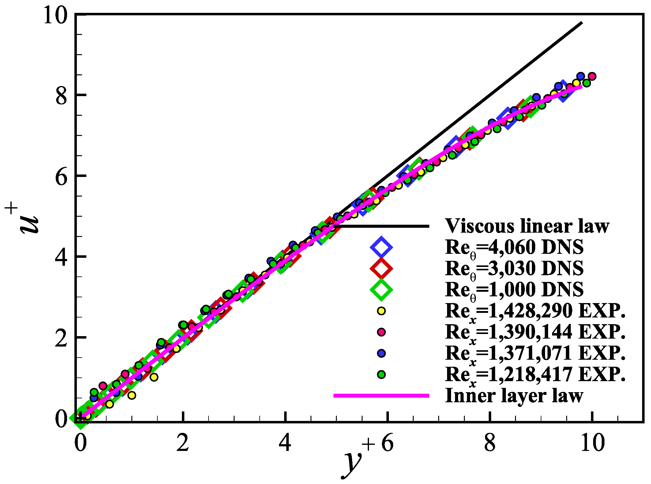
3.1. Validation of the Effectiveness of the Inner Layer Law

For the sake of clarity, only the representative experiment (EXP.) data and the DNS results are presented in the following figures. Figure 1 provides the DNS results (hollow diamonds) together with the EXP. measurements (solid circles) from the PIV equipped with the single pixel ensemble correlation (SPEC) which is explained in detail in Section 4, the data are distinguished by the different colors and symbols in the graph. These DNS and EXP. data in Figure 1 are benchmarked by the traditional linear law of Equation (1) and the newly developed law of Equation (13) in the inner layer (hereafter called the inner-layer law). The EXP. and DNS results consistently confirm with each other through their good agreements within the inner layer of $y^{+}\le 9.8$. In the viscous sublayer of $y^{+}\le 4.3$, the DNS and EXP. data are quite well in line with both the viscous linear law and the inner-layer law.

It is worth noting that traditionally, the upper limit of viscous sublayer often varies slightly in the literature, and generally speaking, the limit was widely accepted in the range of $y^{+}$ from 4.0 to 5.0. However, under the framework of the current wall-law development in Wang and Xu [5,7], all the near-wall sublayers, up to the log-law layer, were rigorously defined by the indicator function (IDF). It was found that the viscous and inner sublayers were well identified by the IDF’s inflection and extreme points. Thanks to the similarity of ZPGFP TBL, the upper limits of these sublayers were quantitatively pin-pointed to a quite universal value of $y^{+}$ equal to 4.28 and 9.8 for the viscous and inner sublayers, respectively. Therefore, the maximum relative error of deviation from the viscous linear law is less than 2% within $0.0<y^{+}\le 4.3$, which is reliably calibrated based on the existing DNS and EXP. data. Meanwhile, both the DNS and EXP. results, as seen in Figure 1, consistently agree well with the inner-layer law of Equation (13) in $0.0<y^{+}\le 9.8$ and the data gradually deviate from the linear law in the region of $4.3<y^{+}\le 9.8$ where the traditional viscous linear law is no longer suitable and applicable. As explained in the existing literatures, the reason is attributed to the fact that the turbulence shear stress of $\overline{u^{\prime }{v}^{\prime }}$ emerges at the location of $y^{+}=4.3$ and grows rapidly which makes the velocity profile deviate from and be suppressed comparing to the viscous linear law.

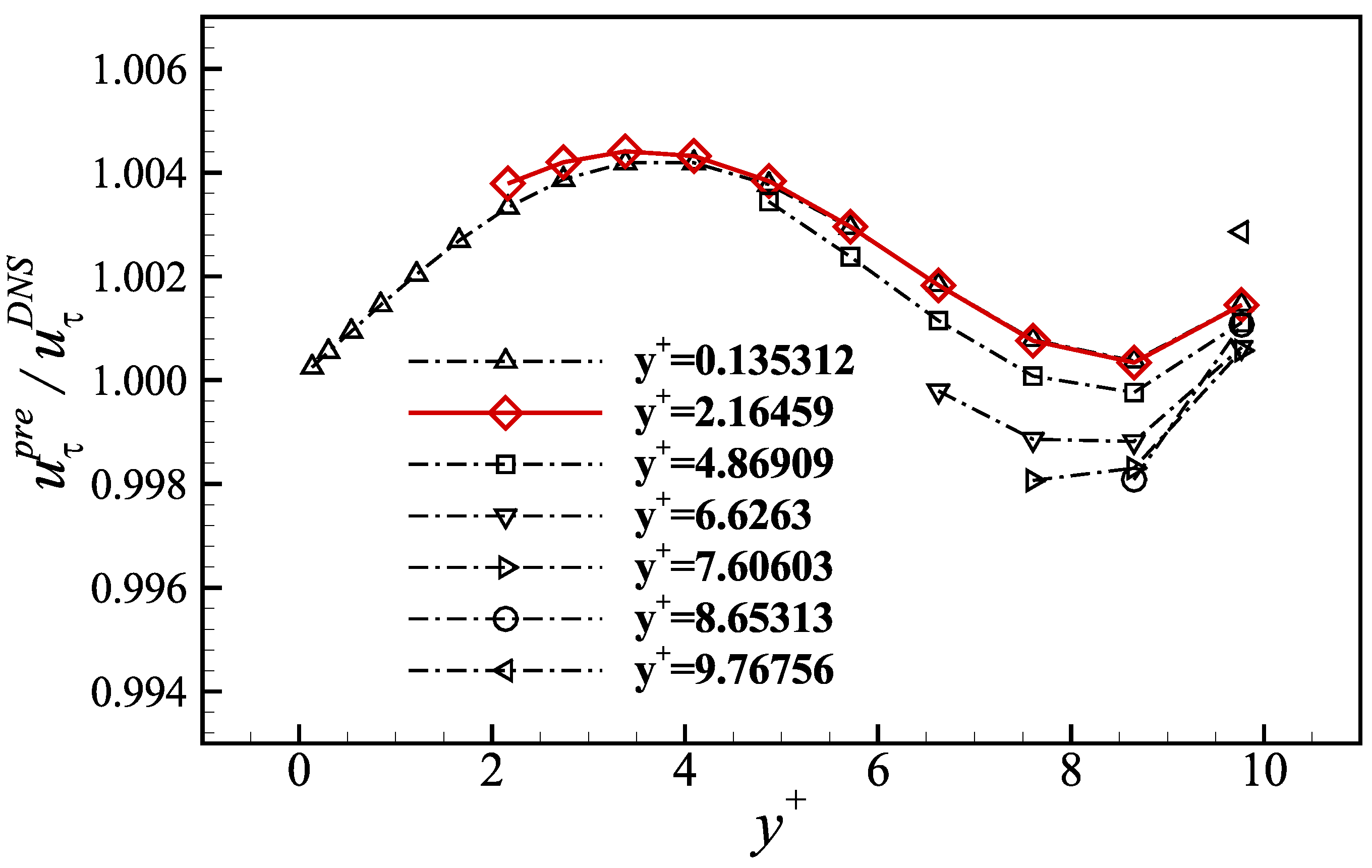
3.2. Prediction Accuracy of the Proposed Method for Estimating WSS

Based on the DNS data with ${Re}_{\theta }=3030$, a total of seventeen data sets in the range of $0.0<y^{+}\le 9.8$ are provided. Five of these data fall in $0.0<y^{+}\le 1.0$, as seen in Figure 2, which are considered rigorously satisfying the viscous linear law. Therefore, the local frictional velocity of $u_{\tau }^{DNS}$ can be calculated and determined based on these five data sets as a benchmark. As well-known, the least squares method (LSM) is usually applied to process the data in an experiment to reduce the measuring error. Hence, in order to mimic an experimental condition, the current study makes use of the DNS data in the various $y^{+}$ ranges with the different low and upper limits as presented in Figure 2, and then applies the LSM to these data to obtain the predicted local frictional velocity of $u_{\tau }^{pre}$ using $u=\left(u_{\tau }^2/v\right)y$ which is normalized by $u_{\tau }^{DNS}$ in Figure 2a. The horizontal and vertical axes in Figure 2 stand for the wall distance of $y^{+}$ and the the normalized local frictional velocity of $u_{\tau }^{pre}/u_{\tau }^{DNS}$, respectively, whereas the legends in figure provide the wall-distances of the first data point or the low-limit information and the data points on same curve represent the group of fitted data having the same low limit.

Except the first point, the data points on the same curve stand for the group of least-square fitting points with their corresponding upper limits represented by the horizonal axis values. For the sake of presentation clarity, only six representative curves in the total of seventeen curves, denoted by the red dots in the matrix, are selected in the plots with the pattern of curves being displayed by the solid and solid-dot lines alternatively.

On one of these curves with an identical low limit, the prediction accuracies monotonically decrease since $u_{\tau }^{pre}$ tends to deviate from $u_{\tau }^{DNS}$ when their upper limits increasing or when the data point moving towards right along the curve as indicated in Figure 2a. On the other hand, when talking about the various curves with the different low limits, the prediction accuracies become worsen when the low limit increasing or when the first data point moving away from the wall. The first point on each curve provides the accuracy based on single measuring point while the other points on the same curve presents the accuracies using multiple-points based on the LSM.

From Figure 2a, it can be found that the curve with $y^{+}=0.135312$ provides the almost perfect accuracies for $u_{\tau }^{pre}$ in the region of $0.0<y^{+}\le 1.0$ since $u_{\tau }^{pre}/u_{\tau }^{DNS}\approx 1.0$. The prediction accuracy monotonically decreases when either the data-fitting upper limit increasing or the data-fitting low limit rising. When studying the data in $0.0<y^{+}\le 5.0$, the $u_{\tau }^{pre}$ is generally under estimated with a maximum error at about $1.5\%$ comparing to the $u_{\tau }^{DNS}$. The same observation with a maximum error at $7.1\%$ can be obtained when looking at the data in $0.0<y^{+}\le 9.8$. These studies provide a conclusion that the prediction accuracy can generally be improved when the data point getting closer to wall. However, the measuring accuracy in a real experiment is usually found contradictorily getting worse when the data point approaching closer to the wall. The reasons are provided as following, which calls for a more accurate wall-law prediction capability.

For the medium-to-high range of $\mathrm{Re}$, the current mainstream measurement technology is generally capable of obtaining the near-wall data with a reliable accuracy at a minimum wall distance of $y^{+}\approx 2$ as exhibited by the curve in Figure 2a, which is represented by the enlarged left triangle symbol with the dotted line. However, regarding to the flows in the range of a high to ultra-high Re for engineering practice, it is very difficult, if not impossible, to obtain the data points down to the wall distance of $y^{+}=2$, since the dimensional thickness of the boundary layer becomes extremely thin at the Re, or as shown by the curves in Figure 2a, the data points are so scarce that makes the measurements unreliable.

Nowadays, the popular measurement technologies, such as the PIV, the single-point LDV and HW, are all facing the issue of extreme-wall-distance measurement, or the measured wall distance is generally deviated from the absolute wall position in reality. Therefore, it is no longer appropriate to fit the measured data with the linear function [26] of $u=\left({u_{\tau }}^2/\nu \right)y$. Instead, it is suggested that the data be fitted with an offset linear function [29] $u=\left({u_{\tau }}^2/\nu \right)(y-b)$, with the parameter b representing the overall offset of the wall distance and being determined by the LSM. The prediction accuracy using the offset linear function is given in Figure 2b, and the meanings of various elements (points, lines, coordinate axes) in the picture are consistent with those in Figure 2a.

Regarding the curve in Figure 2b, as the upper limit increases, the prediction accuracy decreases monotonically and more rapidly comparing to the corresponding one in Figure 2a. As the low limit of fitted data increases, see the various curves in Figure 2b, the prediction accuracies are also getting worsen quickly. When the fitting data are in $0.0<y^{+}\le 5.0$, the $u_{\tau }^{pre}$ is generally underestimated, and the maximum error can increases up to 5%. However, the prediction in the interval of $5.0<y^{+}\le 9.8$ can even be more underestimated with the maximum error reaching up to 23% in the extreme situation. Comparing Figure 2a to Figure 2b, it can be found that the linear-function fittings, with the wall location pre-defined, generally outperform the accuracies from the offset linear function, which is evidently attributed to the issue of the absolute-wall distance in an experiment measurement.

Therefore, it can be summarized that the wall-slope method based on either the linear function or the offset linear function can maintain a good accuracy in evaluating the local friction velocity or wall shearing stress in the region of $0.0<y^{+}\le 5.0$, because the velocity distribution in the region well satisfies the viscous linear law. However, for a higher Re flow, the measurement point can hardly get into the region of $0.0<y^{+}\le 5.0$, which causes the wall-slope method invalid. Therefore, a more accurate wall-law model is highly demanded, which can be applied to the region beyond the applicable range of the current viscous linear law.

Within the context, the inner-layer law of Equation (22) in the current study is further applied to predict the local frictional velocity based on the DNS results at ${Re}_{\theta }=3030$. These predictions of the local frictional velocity are presented in Figure 3 in a normalized form, which demonstrates the excellent predicting capability with the relative errors generally below 0.5%.

As is well-known, an accurate velocity profile within the layer of $0<y^{+}\le 2$ is quite difficult to be acquired in an experiment. Because the velocity in the sublayer is very tiny, the measurement errors of device become particularly pronounced in the region, which is bound to lead a large discrepancy from the accurate answer. Hence, the results in the layer of $2<y^{+}\le 9.8$ are used in the following analysis to verify the validity of the current measuring method and the validations are highlighted in Figure 2 using the bold symbols of left triangle on dash-dot line and in Figure 3 using the red diamond symbols on red line, respectively.

Figure 4 illustrates the comparison of the predictive accuracy between fourth-order polynomials, fifth-order polynomials, linear laws, and inner-layer law across various $y^{+}$ ranges. When utilizing data within the $y^{+}<2$ range, the fifth-order polynomial yields the highest predictive accuracy. Conversely, for data within the $y^{+}>2$ range, the inner-layer law demonstrates superior predictive performance. As the upper limit of the data range increases, the accuracy of both polynomial and linear predictions decreases, whereas the inner-layer law’s predictive accuracy does not diminish. Comparing the predictive accuracy of different methods at varying lower limits reveals that the accuracy of polynomial and linear predictions is sensitive to the lower limit of the data range, whereas the inner-layer law exhibits better robustness.

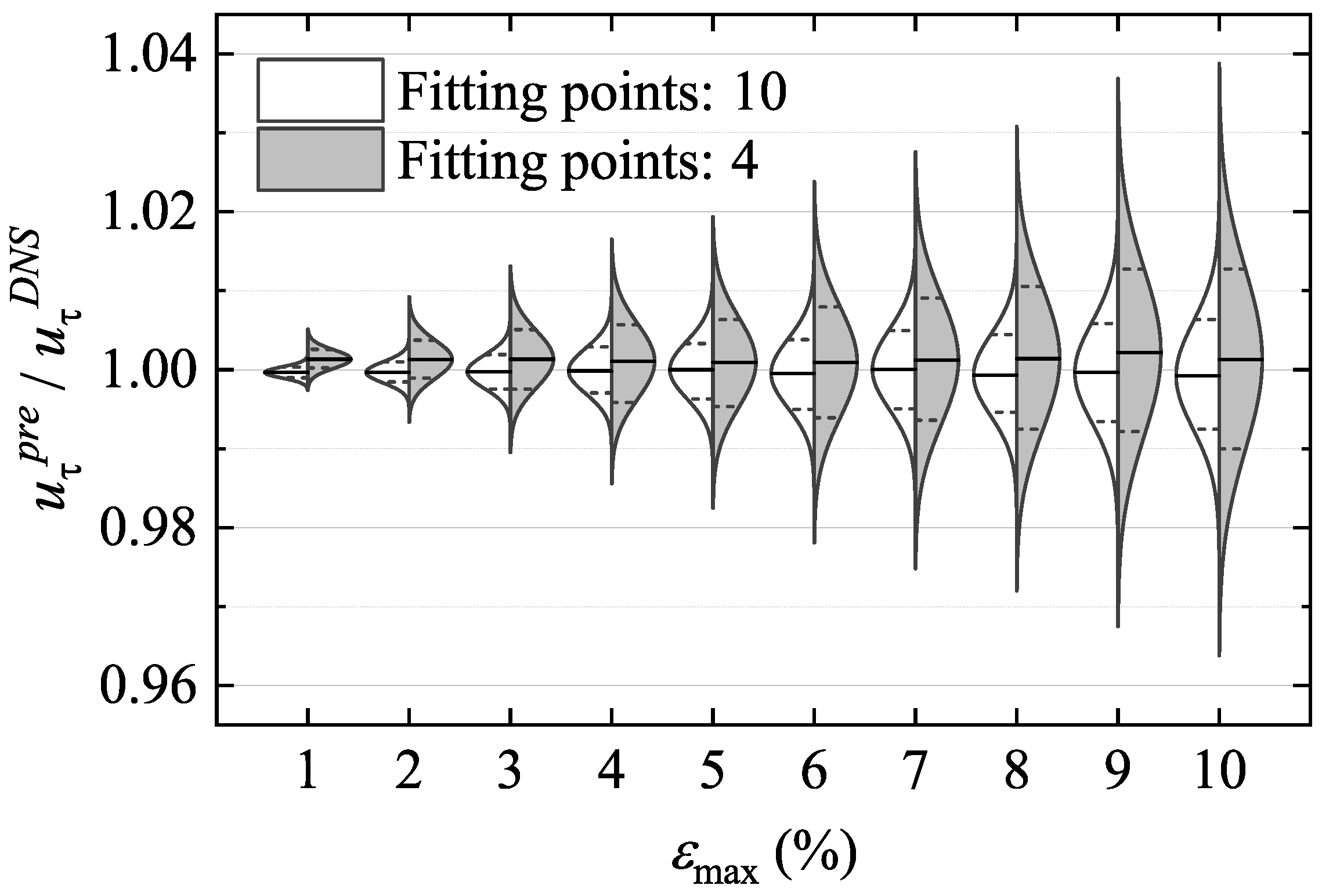
3.3. Evaluating the Proposed Method under Systematic and Random Errors

It is well recognized that experimental results are subjected to a variety of random and systematic errors [34]. In order to verify the accuracy and robustness of the method in an experiment, some random and systematic errors were imposed on to the DNS results to simulate the real experimental data. A procedure was conducted for imposing a Gaussian random signal onto an ideal velocity data (DNS), since the random errors are bound to arise in a velocity measurement. Next, a random Gaussian velocity $u=N\left(\mu ,{\sigma }^2\right)$ was generated with the mean value $\mu =u_{DNS}$ and the standard deviation of $\sigma =\left|{\epsilon }_{max}\right|u_{DNS}/3$, where ${\epsilon }_{max}$ denotes the maximum possible relative error defined as ${\epsilon }_{max}=\left(u-u_{DNS}\right)/u_{DNS}$. It is worth noting that the $\mu$ here refers to the mean value of the normal distribution, instead of the dynamic viscosity normally used in fluid mechanics. Based on the 3-sigma principle, about $99.7\%$ of the velocities drawn from a normal distribution are within the three standard deviations of $\sigma$ away from the mean and therefore, the coefficient is taken to be $1/3$.

For a specified maximum error ${\epsilon }_{max}$ of velocity measurement within the range $2.16<y^{+}\le 9.8$, the fitting procedure using Equation (22) was repeated 500 times for the different random signal. A fitted gaussian density function is then used to describe the distribution of predicted local friction velocity, as shown by the curves in Figure 5, where the straight solid line and dashed line represent the mean value and the one standard deviation of, respectively, based on the corresponding probability density function. The predictive accuracy of the method was also analyzed via investigating the influence of the fitting-point number on the results, as given in Figure 5, where the white shaded part (left part) and grey shaded part (right part) stand for the predicted results from the ten and four measuring points, respectively, abbreviated as Case-10 and Case-4.

There are ten DNS velocity data in the interval of interest, and Case-10 deals with all data in the interval while Case-4 deals with the data with a spacing of 3. For Case-10, it can be concluded that the local frictional velocities estimated from the randomly perturbed velocity profiles present the deviations from their true value and the deviation ranges become wider with the increase of ${\epsilon }_{max}$. However, these deviations can always be maintained at a quite low level within the acceptable tolerance of engineering applications. For ${\epsilon }_{max}\le 10$, the maximum relative error is less than $2\%$, and the one-sigma data are distributed within the relative errors of $0.8\%$. For the data with ${\epsilon }_{max}\le 5$, the maximum relative errors can be kept within $1\%$ and the one-sigma data are distributed within the relative errors of $0.5\%$. Comparing the Case-4 to Case-10, smaller number of fitted points make the possible prediction deviation larger and the prediction more divergent. However, the mean values of these prediction all exhibit an excellent prediction accuracy. For ${\epsilon }_{max}\le 10$, the maximum relative error is less than $3.9\%$, and the one-sigma data are distributed within the relative errors of $1.3\%$. For the data with ${\epsilon }_{max}\le 5$, the maximum relative errors can be kept within $1.9\%$ and the one-sigma data are distributed within the relative errors of $0.7\%$.

In TBL experiment, the measurement error of the absolute wall position can be regarded as a systematic error and a pre-offset $y_0$ parameter is imposed onto the ideal position of y to represent the error. Simulating processes with both systematic errors and random errors can help evaluate the overall accuracy and precision of the measurement process. As shown in Figure 6, the DNS data with random error and systematic error was analyzed using Equation (23).

Although the PIV measurement accuracy is generally less than $2\%$, a maximum error of the velocity measurement is specified at ${\epsilon }_{max}=5$, since the measuring error in the near-wall region is usually greater than the measurement accuracy in the far field. Since the wall-law model contains two parameters to be estimated for the test, the minimum number of two data points are needed in the wall sublayer. Practically speaking, the current measuring technique, such as a PIV or a HW method, is capable of obtaining the flow data of around three or four points within the near-wall sublayer. Therefore, the current study selects the DNS data at four probing points within the inner layer to simulate the reality situation in experiment. In Figure 6, for a specified systematic error pre-offset, set maximum random error ${\epsilon }_{max}=5$ and predict the WSS using Equation (23) within the range $2.16<y^{+}\le 9.8$. The fitting procedure was repeated 500 times with different pre-offset $y_0$. A fitted gaussian density function is used to describe the distribution of predicted friction velocity, as shown in Figure 6, curve, diamond shape and vertical bar indicate probability density distribution, mean value and one standard deviation of the predicted results, respectively. It can be seen that in extreme cases, the maximum relative errors can be kept within $5\%$ and the one-sigma data are distributed within the relative errors of $1.8\%$. Meanwhile, the relative error is insensitive to systematic error (absolute wall position).

4. Applying the WSS Estimation Approach to a TBL Experiment

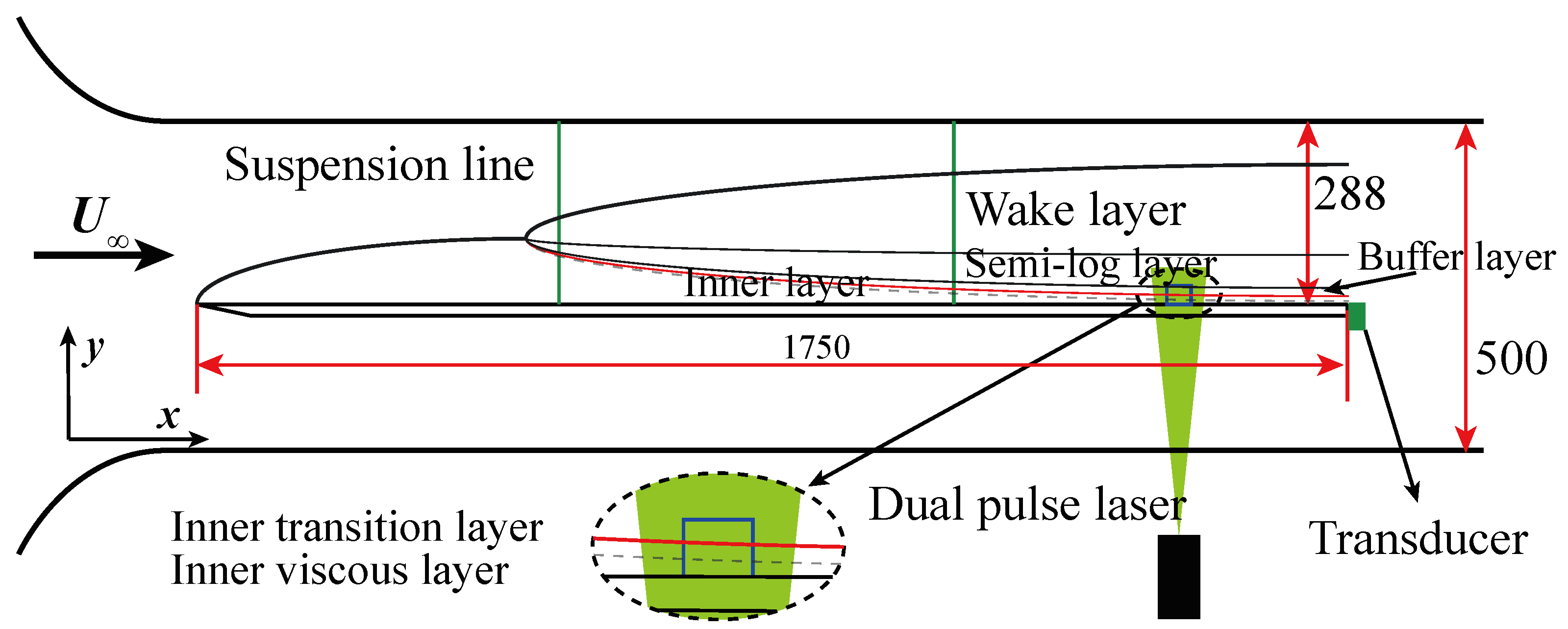
4.1. Experimental Setup

The test rig was setup and schematically shown in Figure 7. The experiment was conducted in a low-speed recirculation wind tunnel of Fudan University, which was equipped with a test section of 0.5 m (width) by 0.5 m (height) by 2 m (length) and the wind speed range in 4–50 m/s. A smooth acrylic flat panel of 1.750 m (length) by 0.3 m (width) by 15 mm (thickness) was built to generate a canonical smooth-flat wall TBL. Its leading edge was made a wedged shape to avoid local flow separation. As illustrated in the figure, the panel was suspended horizontally from the top wall of the wind-tunnel test section by four 0.5 mm diameter steel wires to minimize their flow interference. The flat plate was gaped at 0.288 m from the top wall of wind tunnel, which was considered as large enough to avoid the wall effects and was confirmed by the boundary layer with a thickness of less than 0.06 m in the testing condition.

A force transducer (SBT431-300g, Simbatouch, Guangzhou, China) was flexibly mounted downstream the flat plate, with the transducer’s surface touching the tail of flat plate and the other end attached to the bottom wall of the wind tunnel. The sensor possesses a measurement range of $3\mathrm{N}$, a resolution of $0.001\mathrm{N}$, and a dynamic frequency response of $450\mathrm{Hz}$. Prior to the experiment, the sensor was calibrated both online and offline using the standard weights. The force sensor measured the total WSS acting on both the upper and lower surfaces of flat plate.

In the experiment, the wind speed was set at $14.5\mathrm{m}/\mathrm{s}$ and the flat plate was set under the surveillance of a camera with a magnifying power. The flat plate in the entire experiment was found not experiencing any visible vibration at the given wind speed. The first measurement point was $1.255\mathrm{m}$ downstream the leading edge where the Reynolds number was ${\mathrm{Re}}_x=1.2\times {10}^6$. The TBL in the mid (x–z) plane normal to the flat plate was measured by the 2D PIV technique. For the PIV measurement, the flow field was seed by the oil-droplets with a median diameter of 1 $\mathsf{\mu }$m. The illumination was a dual pulsed laser sheet with a thickness of $1\mathrm{mm}$ produced by a Nd:YAG laser generator (Beamtech Vlite-500, Beamtech Optronics, Beijing, China) at an energy output of 200 mJ/pulse. A 12-bit charge-coupled device (CCD) camera was used together with a Nikkon lens, which could capture the flow field at a resolution of 2456 pixels × 2058 pixels. The field of view (FOV) was a window of $23.95\mathrm{mm}\times 20.07\mathrm{mm}$. The time interval between the image pairs was set at 6 $\mathsf{\mu }$s and the frequency was at $5\mathrm{Hz}$.

The velocities were measured at the 17 locations successively starting from the first measuring spot at x = 1.255 m. The spacing between two adjacent measuring points was $20\mathrm{mm}$, slightly less than the FOV. The movement of the camera and laser along the flow direction was controlled by the displacement platform with a controlling accuracy of $0.03\mathrm{mm}$. In the experiment, a force balance method was applied to measure the ensemble-averaged (spatial-temporal mean) WSS of fully developed TBL, since the ensemble-averaged WSS was pin-pointed as an important parameter in the wall-law development [5,7]. To cleanly eliminate the effects of laminar and transition regions upstream the measuring locations, a flat plate at a shorter length of 1.255 m was separately applied and therefore, via the subtraction of two measurements, the ensemble-averaged net wall friction can be obtained accurately for the WSS in a fully developed turbulence section.

4.2. Results and Analysis

During the experiment, the measurements of flow field were taken on the plate upper surface based the minimum disturbance criteria due to two reasons. Firstly, the leading edge of flat plate was designed with a lower-surface wedged shape and secondly, the plate was suspended by the strings mounted at the holes on the lower surface presented by Figure 7 and Figure 8.

Figure 8 provides an example of near-wall snapshot of the particle images with the yellow line representing the absolute wall position and the red vector line symbolically standing for streamwise velocity profile satisfying the viscous linear law. This figure demonstrates the particle concentration in the PIV experiment and the quality of the measuring data, which guaranteed the accuracy of the subsequent measurements and the reliability of the analyses. There are two ways to ascertain the absolute wall position [26], namely the extreme value of the velocity distribution and the image processing method. To meet requirement of a PIV experiment, the testing model was made of the light-transmitting materials. On the wall surface, the minimum-speed restriction had to be imposed due to the optical reflection effects from the model, such as an Acrylic material. Although the Gaussian peak finding approach [21,31] can be applied to improve the accuracy, the image processing methods are generally utilized to give the information of absolute wall position, since the current experiment setup eliminated the model’s vibrations.

To determine the absolute wall position, Figure 9 displays the dimensional velocity distribution in the near-wall region when the ${Re}_x$ being equal to 1.1 million. The y-axis denotes the spatial location in terms of the pixels, while the x-axis represents the dimensional velocity. The original velocity data are represented by the red dots from the PIV measurement. The near-wall velocity, including the original and the mirrored one, can be linearly fitted by the two black-dashed lines in the figure. Albeit not reaching an exact zero-velocity point, it is apparent that the velocity roughly reaches a local minimum in the vicinity of pixel position at 1867. Based on velocity-extremum method, however, the Gaussian peak-finding technique is utilized to determine a more accurate the absolute wall position, which is derived at the pixel location of 1867.6. Meanwhile, the near-wall linear-velocity distribution represented by the black-dash line confirms the viscous linear law in the wall viscous sublayer. The wall position, as determined by both the image-processing method and the velocity based methods, was found being in pretty good agreement.

The traditional PIV method using interrogation window (IW) has presented its reliable robustness and rare outlier data in a variety of practical applications, since the method is able to collect the sufficient optical information to capture flow field. However, the method is encountered a serious issue in terms of its spatial resolution, particularly in a near-wall TBL due to the wall interference on the optical ray in PIV and the velocity gradient, which poses an almost insurmountable difficulty in estimating a WSS using the near-wall PIV velocity data. To improve the PIV spatial resolution, the variants of IW-based PIV, i.e., SPEC technique, was applied for image pairs post-processing [35].

In SPEC, IW is reduced to 1 × 1 pixel. The reduced spatial information in the domain is then compensated by the ensemble averaging the cross-correlation map in time, which typically needs ensemble thousands of images pairs for a distinct correlation peak with the sufficient signal-to-noise (SNR). In the current study, the image pairs up to 2100, equivalent to 4200 images, were used to compensate the optical information, although practically speaking, the satisfying results were able to be obtained by 1500 image pair. The PIV system in the experimental device discussed was able to acquire 75 image pairs per cycle, and the device repeated to take images for 28 times at each measuring point.

As seen in Figure 10a, all the streamwise velocity profiles collapse together due to the well-known similarity for ZPGFP TBL. The current experimental data (circles) agree well with the hot-wire measurements (squares) from the KTH laboratory [36] and the DNS results [37]. The current experiment was carried out under the condition of equidistance, whereas the measurement points in the hot-wire experiment are non-equidistance because of the logarithmic coordinates employed. According to the hot-wire experiment data, the measuring point closest to the wall was roughly at the position of $y^{+}=13$. However, the measuring point in the current PIV can detect the PIV tracing particles down to $y^{+}=1$ or even below. Although PIV tracing particles, in theory, are able to reach the very near-wall region, the measuring errors in the region are usually large due to the wall interference effects on the optical signal. The current experiment demonstrates that the relative errors can exceed 15% in $y^{+}=1$, while the PIV errors is less than 2% in the measurements of other areas outside $y^{+}=1$. The detailed results in the near-wall region are shown in Figure 1, and it can be seen that as $y^{+}$ increases, the velocity gradually deviates from the linear law. It can be seen that in the log region, the log law exists, and the additional value of the log law is slightly different.

As seen in Figure 10b, the velocity profile displays a cluster of curves when the dimensionless scale is selected as the ensemble-averaged friction velocity $\overline{u_{\tau }}$. The conventional wall-law employs the local WSS as the dimensionless scale, which implicitly include the local frictional velocity $u_{\tau }$ or WSS into the independent variables and thus the derived wall-law becomes Reynolds number independent. However, if the ensemble-averaged $\overline{u_{\tau }}$ or WSS is employed as the velocity scale, the correlation between $u_{\tau }$ and Reynolds number needs to be explicitly expressed. The each one of the clustered curves in Figure 10b represent the velocity profiles at different x-locations of ${Re}_{\theta }$ scaled by $\overline{u_{\tau }}$. The current experimental data (circles) agree well with the DNS results when ${Re}_{\theta }$ being equal to 1000. The hot-wire experimental data (diamonds) agree well with the DNS results at the ${Re}_{\theta }$ equaling to 2540 and 3970. The concept of utilizing the ensemble-averaged, or the spatial-temporal averaged friction velocity as the dimensionless scale not only enables the comparison of data obtained from various sources, but also facilitates the computation of the WSS. The family of curves in Figure 10b represent velocity profiles originated from the different ratios between the local WSS and the ensemble averaged WSS.

Figure 11 displays the variation of dimensional friction velocity with the Reynolds numbers based on streamwise locations of x, namely ${\mathrm{Re}}_x$. The predicted friction velocity (black diamonds) calculated by Equation (23) decreases with increasing ${Re}_x$. The green dashed line represents the ensemble-averaged friction velocity measured by the force transducer, which is described in detail by Figure 11. As can be seen from Figure 11, the predicted friction velocity ranges from 0.538 to $0.522(\mathrm{m}/\mathrm{s})$, corresponding to the dimensionless friction-velocity ranging in $(0.99,1.02)$, as shown in the subfigure. The local friction velocity calculated by Equation (23) is distributed in the proximity of measured ensemble-averaged friction velocity. The strong agreement between the local $u_{\tau }$ calculated by Equation (23) and the measured ensemble-averaged of friction velocity provides compelling evidence to support the reliability and robustness of the current approach. Additionally, the monotonically decreasing $u_{\tau }$ with the increasing Reynolds number is in quite line with the TBL physics and the reported data in the existing literatures.

As seen in Figure 12, the force measurement process is composed of the five distinct stages. The first stage is the zero-load stage, denoted by the red symbols, which refers to the state before the wind tunnel starts running. The second stage is the loading stage, denoted by the green, corresponding to the startup process of the wind tunnel. The next is the load stage, denoted by the blue, when the tunnel reaching a steady working condition. The fourth stage is the unloading stage, denoted by black, corresponding to the process of reducing the load to zero before the wind tunnel stops running. The final stage is the post-unloading stage, denoted by the orange, corresponding to the state after the wind tunnel stops operating.

The net friction is determined by subtracting the average of the force during the zero-load stage and the post-unloading stage from the force during the load stage. In the experiment, the net force for the test model with long streamwise length is $0.87\mathrm{N}$ and for the one with short streamwise length is $0.77\mathrm{N}$. Therefore, the wall friction in the turbulent region is determined at $0.10\mathrm{N}$ by eliminating the force induced by the upstream plane which is equivalent to the force generated by the model with the short streamwise length.

The load stage lasted for 17 s in the force measurement process. The sampling duration was chosen to ensure that the measurements data achieved the convergence. The process was segmented into the two distinctive substages, namely (1) the initial load stage (0–8 s) and (2) the stable load stage (8–17 s), with the statistical parameters for each substage being detailed in

Table 1. Statistical parameters of load stage.

Stage	$\mathit{\mu }$	$\mathit{\sigma }$	${\mathit{c}}_{\mathit{v}},\%$
Initial Load Stage	109.81	0.26	0.24
Stable Load Stage	109.82	0.03	0.03

. The data suggest that the mean values of $\mu$ in these two substages exhibited remarkable consistency, with a relative deviation of less than one ten-thousandth. Furthermore, a comparison of the standard deviations $\sigma$ between the two substages exhibits that the stable load stage has a lower standard deviation, corresponding to a coefficient of variation $c_v$ of 0.03%. The finding indicates that the data achieved a steady state and convergence within the given sampling duration.

5. Applying the WSS Estimation Approach to Higher Re TBL

The wall-bounded turbulence is generally at a relatively high Reynolds number (Re) in practical engineering applications. Based on the wall-law predictive capability (Re-independency), it is confident that the current method proposed in the paper can be pushed to the high Re regime. The WSS was measured independently using the oil-film approach in the TBL database shared by KTH [38]. Although the method can slightly interfere with the wall in theory, it is still currently recognized as a relatively accurate method that can be used as a benchmark. The velocity is measured using a hot-wire anemometer, and the relatively sparse data in the inner layer are also suitable for verifying the reliability of the current method.

Figure 13 presents a variety of DNS and experimental data, including the squares standing for the DNS data, the diamonds for existing experimental data, and the circles for the current experimental results. The hollow shapes are obtained from the data in the existing literatures, and the solid shapes represent the results predicted by the current proposed method. The dotted line indicates the commonly used friction coefficient curve well-known as the friction law, which is produced based on the Coles-Ferobolz formulation [39] and is revised by combining the new experimental results, For the details, please refer to Reference [40]. Due to the completeness of the DNS data, shown by the green symbols in Figure 13, the predictions from the current method agree well with the DNS friction coefficient data. The detailed quantitative error estimation $E{r}_{\mathrm{D}\mathrm{N}\mathrm{S}}=\left|{C_f}_{\mathrm{L}\mathrm{a}\mathrm{w}}-{C_f}_{\mathrm{D}\mathrm{N}\mathrm{S}}\right|/{C_f}_{\mathrm{D}\mathrm{N}\mathrm{S}}$ is given in

Table 2. Relative error $Er$ of ${C_f}_{\mathrm{LAW}}$ compared with ${C_f}_{\mathrm{DNS}}$ and ${C_f}_{\mathrm{OFI}}$.

$\mathit{Er}$	${\mathit{Er}}_{\mathbf{mean}},\%$	${\mathit{Er}}_{\mathbf{max}},\%$	${\mathit{Er}}_{\mathbf{min}},\%$
$E{r}_{\mathrm{DNS}}$	0.108	0.131	0.0496
$E{r}_{\mathrm{OFI}}$	1.790	5.700	0.0252

where the maximum error $E{r}_{\max }$ is at $0.131\%$ and the average error $E{r}_{\mathrm{mean}}$ is about $0.108\%$. The data in the purple symbols are in the region of the medium to high Re. Evidently, the predicted WSS represented by the frictional coefficients agree consistently with the oil-film data for high Re. Due to the gradual thinning of TBL at a high Re, it is more difficult to measure the velocity information in the near wall region using a hot wire since only one or two measurement points can be placed inside the region. However, the current approach, even under this harsh circumstance, can still give an accurate prediction acceptable to engineering requirement. The detailed quantitative error estimation $E{r}_{\mathrm{O}\mathrm{F}\mathrm{I}}=\left|{C_f}_{\mathrm{L}\mathrm{a}\mathrm{w}}-{C_f}_{\mathrm{O}\mathrm{F}\mathrm{I}}\right|/{C_f}_{\mathrm{O}\mathrm{F}\mathrm{I}}$ is given in Table 2 where the average error $E{r}_{\mathrm{mean}}$ is about $1.790\%$, and the maximum error $E{r}_{max}$ is maintained below $5.70\%$ even when the data are being obtained by only one nearwall point in the measurement.

6. Conclusions

1.

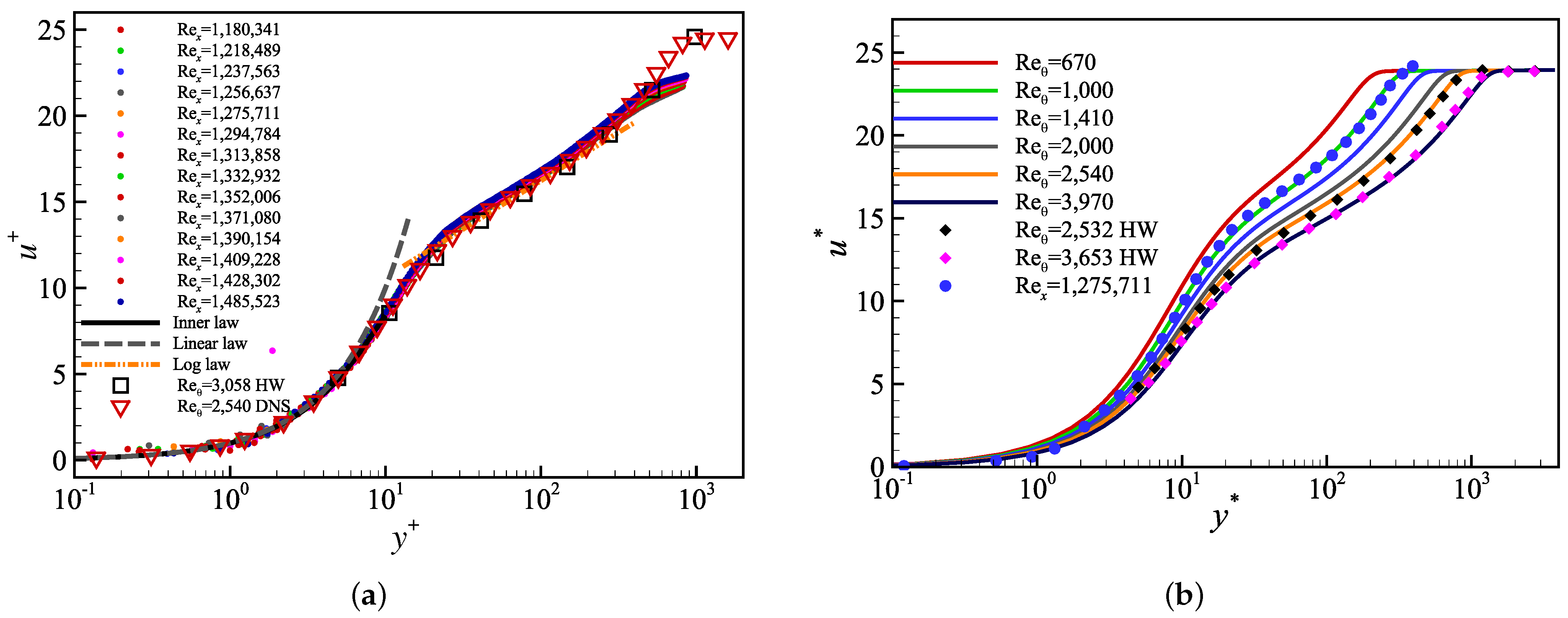
The PIV technique, combined with the high spatial resolution post-processing method SPEC, was applied in the current study to measure the near-wall velocity profile in a ZPGFP TBL and about 24 velocity points were captured in the TBL inner-layer region $\left(y^{+}<9.8\right)$ as defined by Wang [5]. These measurements, along with the current DNS data [37], solidly validated the effectiveness of the inner-layer law formulation in accurately describing both the velocity profile and its derivative in the layer.

2.

A novel non-intrusive method was then developed and proposed for an accurate estimation of WSS based on the near-wall mean velocity measurement and the newly derived analytical wall-law. The WSS prediction accuracy based on the current approach is almost an order of magnitude higher than the existing methods if the velocity can be precisely determined in inner layer. In contrast to the linear wall-slope method, the current approach demonstrated its evident advantage in term of reducing the near-wall velocity measuring difficulty and relieving the high demand for the measuring precision of an experimental instrument. Additionally, the method is relatively insensitive to the absolute wall position. Comparing to the polynomial prediction method for WSS, the current approach exhibits a much better accuracy in the region of $y^{+}>2$ with an error consistently less than $0.5\%$. Furthermore, the application scope of the current method is clearly defined by the IDF function, which was well validated in the current experiment. Compared to WSS prediction methods based on the semi-log law, the accuracy of the current method is not affected by the upper and lower bounds of the data interval. The superiorities of the current method over the existing approaches are achieved by the fact that the new TBL wall-law relations are formulated with the minimum number of control parameters possessing their clear physical meanings, such as the damping strength $\left(\epsilon \right)$ and damping distance $\left(D\right)$, and therefore are capable of guaranteeing the continuities of not only the velocity profiles but also the profile’s derivatives even at the transition points of TBL sublayers.

3.

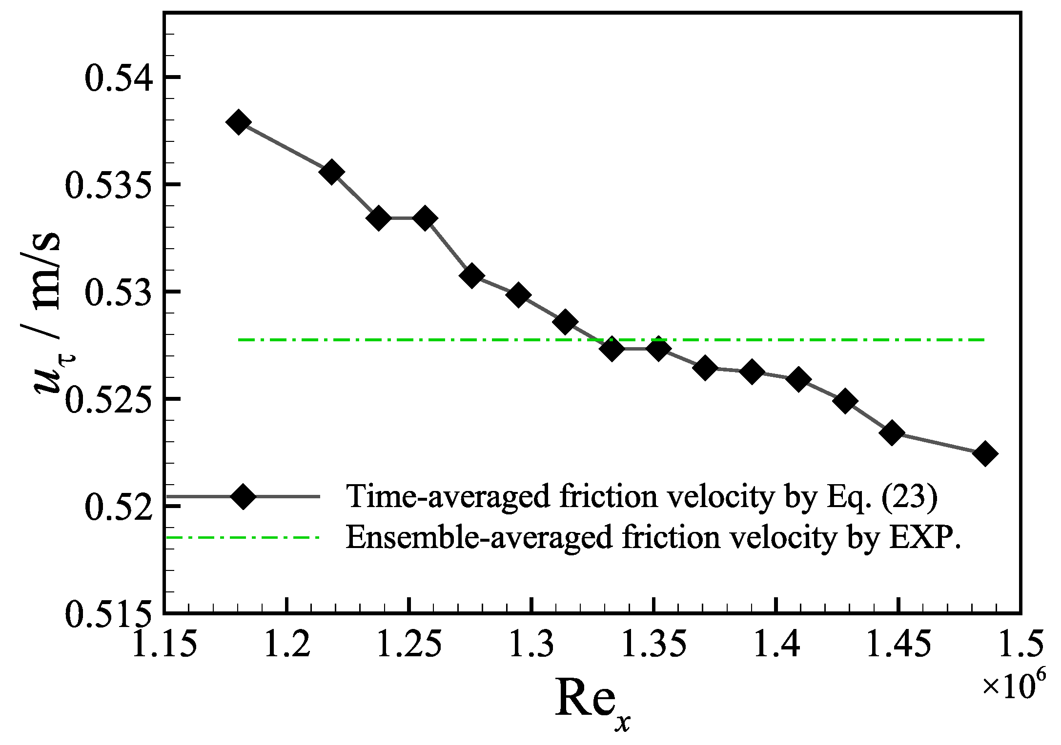
The robustness and reliability of the method was verified by the existing DNS data subjected to random and systematic errors, which proved that the current approach is insensitive to the disturbances in an experimental measurement. The PIV experiment equipped with SPEC was performed for the fully developed ZPGFP (Type-A) TBL at several Reynolds numbers and the collected data were analyzed using the proposed method which presented the accurate predictive capability of both the velocity profile and its derivatives including the WSS. Meanwhile, the SPEC post-processing method demonstrated its suitability for measuring the time-averaged turbulence statistics in a TBL.

4.

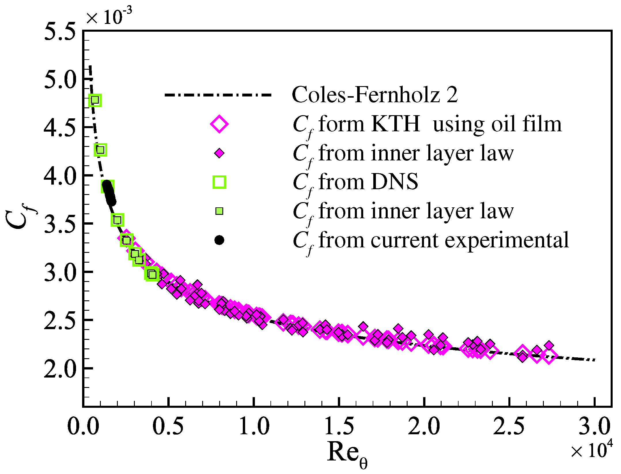
When being applied to the higher Reynolds number TBL data from KTH, the current method provided WSS predictions which exhibited a high degree of consistency with the measurements from the oil film interferometry reported in the literature. Even with very sparse data points, including the instance with only a single data point, the method still presents its superior prediction capability, which evidently suggests that the method possesses the potential to deliver a satisfactory WSS measurement for future engineering applications through using significantly less costly experimental instruments. Moreover, if the current method can be further extended to the wall-law relation in the buffer-layer, i.e., Equation (14), the difficulty in predicting WSS is anticipated to be practically overcome through measuring the near-wall velocity profile, which will be expected to significantly benefit a broad range of fluid engineering applications.

References

1. Prandtl, L. Turbulent Flow; Technical Report Memo. 435; NASA: Washington, DC, USA, 1927. Available online: https://ntrs.nasa.gov/citations/19930090799 (accessed on 20 June 2020).
2. Von Kármán, T. Mechanical Similitude and Turbulence; Technical Report 611; NASA: Washington, DC, USA, 1931; Available online: http://hdl.handle.net/2060/19930094805 (accessed on 20 June 2020).
3. Barenblatt, G. The 1999 James Lighthill Memorial Paper: Scaling laws for turbulent wall-bounded shear flows at very large Reynolds numbers. J. Eng. Math. 1999, 36, 361–384. [Google Scholar] [CrossRef]
4. De Graaff, D.B.; Eaton, J.K. Reynolds-number scaling of the flat-plate turbulent boundary layer. J. Fluid Mech. 2000, 422, 319–346. [Google Scholar] [CrossRef]
5. Wang, D.; Li, H.; Cao, B.C.; Xu, H. Law-of-the-wall analytical formulations for Type-A turbulent boundary layers. J. Hydrodyn. 2020, 32, 296–313. [Google Scholar] [CrossRef]
6. Li, H.; Wang, D.; Xu, H. Improved law-of-the-wall model for turbulent boundary layer in engineering. AIAA J. 2020, 58, 3308–3319. [Google Scholar] [CrossRef]
7. Wang, D.; Li, H.; Li, Y.; Yu, T.; Xu, H. Direct numerical simulation and in-depth analysis of thermal turbulence in square annular duct. Int. J. Heat Mass Transf. 2019, 144, 118590. [Google Scholar] [CrossRef]
8. Cabot, W.; Moin, P. Approximate wall boundary conditions in the large-eddy simulation of high Reynolds number flow. Flow, Turbul. Combust. 2000, 63, 269–291. [Google Scholar] [CrossRef]
9. Saeedi, M.; Wang, B.C. Large-eddy simulation of turbulent flow and dispersion over a matrix of wall-mounted cubes. Phys. Fluids 2015, 27, 115104. [Google Scholar] [CrossRef]
10. Zarbi, G.; Reynolds, A. Skin friction measurements in turbulent flow by means of Preston tubes. Fluid Dyn. Res. 1991, 7, 151. [Google Scholar] [CrossRef]
11. Ruedi, J.D.; Nagib, H.; Österlund, J.; Monkewitz, P. Unsteady wall-shear measurements in turbulent boundary layers using MEMS. Exp. Fluids 2004, 36, 393–398. [Google Scholar] [CrossRef]
12. Schober, M.; Obermeier, E.; Pirskawetz, S.; Fernholz, H.H. A MEMS skin-friction sensor for time resolved measurements in separated flows. Exp. Fluids 2004, 36, 593–599. [Google Scholar] [CrossRef]
13. Naughton, J.W.; Sheplak, M. Modern developments in shear-stress measurement. Prog. Aerosp. Sci. 2002, 38, 515–570. [Google Scholar] [CrossRef]
14. Costantini, M.; Lee, T.; Nonomura, T.; Asai, K.; Klein, C. Feasibility of skin-friction field measurements in a transonic wind tunnel using a global luminescent oil film. Exp. Fluids 2021, 62, 21. [Google Scholar] [CrossRef]
15. Pailhas, G.; Barricau, P.; Touvet, Y.; Perret, L. Friction measurement in zero and adverse pressure gradient boundary layer using oil droplet interferometric method. Exp. Fluids 2009, 47, 195–207. [Google Scholar] [CrossRef]
16. Kendall, A.; Koochesfahani, M. A method for estimating wall friction in turbulent boundary layers. In Proceedings of the 25th AIAA Aerodynamic Measurement Technology and Ground Testing Conference, San Francisco, CA, USA, 5–8 June 2006; p. 3834. [Google Scholar]
17. Mandal, B.; Mazumdar, H.P. The importance of the law of the wall. Int. J. Appl. Mech. Eng. 2015, 20, 857–869. [Google Scholar] [CrossRef]
18. Rodríguez-López, E.; Bruce, P.J.; Buxton, O.R. A robust post-processing method to determine skin friction in turbulent boundary layers from the velocity profile. Exp. Fluids 2015, 56, 68. [Google Scholar] [CrossRef]
19. Wei, T.; Schmidt, R.; McMurtry, P. Comment on the Clauser chart method for determining the friction velocity. Exp. Fluids 2005, 38, 695–699. [Google Scholar] [CrossRef]
20. Marusic, I.; Monty, J.P.; Hultmark, M.; Smits, A.J. On the logarithmic region in wall turbulence. J. Fluid Mech. 2013, 716, R3. [Google Scholar] [CrossRef]
21. Nobach, H.; Honkanen, M. Two-dimensional Gaussian regression for sub-pixel displacement estimation in particle image velocimetry or particle position estimation in particle tracking velocimetry. Exp. Fluids 2005, 38, 511–515. [Google Scholar] [CrossRef]
22. Esteban, L.B.; Dogan, E.; Rodríguez-López, E.; Ganapathisubramani, B. Skin-friction measurements in a turbulent boundary layer under the influence of free-stream turbulence. Exp. Fluids 2017, 58, 115. [Google Scholar] [CrossRef]
23. McEligot, D.M. Measurement of wall shear stress in favorable pressure gradients. In Flow of Real Fluids; Meier, G.E.A., Obermeier, F., Eds.; Springer: Berlin/Heidelberg, Germany, 1985; pp. 292–303. [Google Scholar] [CrossRef]
24. Kendall, A.; Koochesfahani, M. A method for estimating wall friction in turbulent wall-bounded flows. Exp. Fluids 2008, 44, 773–780. [Google Scholar] [CrossRef]
25. Djenidi, L.; Talluru, K.; Antonia, R. A velocity defect chart method for estimating the friction velocity in turbulent boundary layers. Fluid Dyn. Res. 2019, 51, 045502. [Google Scholar] [CrossRef]
26. Wang, J.; Pan, C.; Wang, J. Characteristics of fluctuating wall-shear stress in a turbulent boundary layer at low-to-moderate Reynolds number. Phys. Rev. Fluids 2020, 5, 074605. [Google Scholar] [CrossRef]
27. Shen, J.; Pan, C.; Wang, J. Accurate measurement of wall skin friction by single-pixel ensemble correlation. Sci. China Physics, Mech. Astron. 2014, 57, 1352–1362. [Google Scholar] [CrossRef]
28. Örlü, R.; Fransson, J.H.; Alfredsson, P.H. On near wall measurements of wall bounded flows—The necessity of an accurate determination of the wall position. Prog. Aerosp. Sci. 2010, 46, 353–387. [Google Scholar] [CrossRef]
29. Durst, F.; Kikura, H.; Lekakis, I.; Jovanović, J.; Ye, Q. Wall shear stress determination from near-wall mean velocity data in turbulent pipe and channel flows. Exp. Fluids 1996, 20, 417–428. [Google Scholar] [CrossRef]
30. Adrian, R.J. Particle-imaging techniques for experimental fluid mechanics. Annu. Rev. Fluid Mech. 1991, 23, 261–304. [Google Scholar] [CrossRef]
31. Sugii, Y.; Nishio, S.; Okuno, T.; Okamoto, K. A highly accurate iterative PIV technique using a gradient method. Meas. Sci. Technol. 2000, 11, 1666–1673. [Google Scholar] [CrossRef]
32. Van Driest, E.R. On turbulent flow near a wall. J. Aeronaut. Sci. 1956, 23, 1007–1011. [Google Scholar] [CrossRef]
33. Cao, B.; Xu, H. Re-understanding the law-of-the-wall for wall-bounded turbulence based on in-depth investigation of DNS data. Acta Mech. Sin. 2018, 34, 793–811. [Google Scholar] [CrossRef]
34. Nagib, H.M.; Chauhan, K.A.; Monkewitz, P.A. Approach to an asymptotic state for zero pressure gradient turbulent boundary layers. Philos. Trans. R. Soc. A Math. Phys. Eng. Sci. 2007, 365, 755–770. [Google Scholar] [CrossRef]
35. Kähler, C.J.; Scholz, U.; Ortmanns, J. Wall-shear-stress and near-wall turbulence measurements up to single pixel resolution by means of long-distance micro-PIV. Exp. Fluids 2006, 41, 327–341. [Google Scholar] [CrossRef]
36. Österlund, J.M.; Johansson, A.V.; Nagib, H.M.; Hites, M.H. Wall shear stress measurements in high Reynolds number boundary layers from two facilities. In Proceedings of the 30th Fluid Dynamics Conference, Norfolk, VA, USA, 28 June –1 July 1999; p. 3814. [Google Scholar]
37. Schlatter, P.; Örlü, R. Assessment of direct numerical simulation data of turbulent boundary layers. J. Fluid Mech. 2010, 659, 116–126. [Google Scholar] [CrossRef]
38. Österlund, J.M.; Johansson, A.V.; Nagib, H.M.; Hites, M.H. A note on the overlap region in turbulent boundary layers. Phys. Fluids 2000, 12, 1–4. [Google Scholar] [CrossRef]
39. Fernholz, H.; Finleyt, P. The incompressible zero-pressure-gradient turbulent boundary layer: An assessment of the data. Prog. Aerosp. Sci. 1996, 32, 245–311. [Google Scholar] [CrossRef]
40. Zanoun, E.S.; Nagib, H.; Durst, F. Refined cf relation for turbulent channels and consequences for high-Re experiments. Fluid Dyn. Res. 2009, 41, 021405. [Google Scholar] [CrossRef]
Figure 1. Non-dimensional mean streamwise velocity profiles within 0.0 y + 9.8 for ZPGFP TBL.
Aerospace 11 00544 g001
Figure 2. Normalized WSS prediction based on linear law within 0.0 < y + 9.8 at Re θ = 3030 [29]. (a): u τ p r e is determined by u = u τ 2 / ν y with LSM; (b): u τ p r e and b are determined by u = u τ 2 / ν y b with LSM.
Aerospace 11 00544 g002
Figure 3. Regularized predicted friction velocity using the inner-layer law of Equation (22) within 0.0 < y + 9.8 at Re θ = 3030 .
Aerospace 11 00544 g003
Figure 4. Error analysis of different methods for predicting wall shear stress, 4th-Order Taylor series [29], 5th-Order Taylor series [29], Inner layer law and Wall-slope method. (a): The region y + = 0–10; (b): The region y + = 2.16–10; (c): The region y + = 4.09–10.
Aerospace 11 00544 g004
Figure 5. Regularized predicted friction velocity using Equation (22) at different measurement errors within the region of 2.16 < y + 9.8 .
Aerospace 11 00544 g005
Figure 6. Regularized predicted friction velocity using Equation (23) at different pre-offset y 0 .
Aerospace 11 00544 g006
Figure 7. Schematic illustration of PIV measurement.
Aerospace 11 00544 g007
Figure 8. A snapshot of near-wall particle image with the absolute wall position in the PIV experiments in wind tunnel.
Aerospace 11 00544 g008
Figure 9. Dimensional near-wall velocity distribution.
Aerospace 11 00544 g009
Figure 10. Velocity profiles from the current experimental data with Re x , the experimental data with Re θ [36,38], and from the DNS data with Re θ [37]. (a): Velocity profiles scaled by u τ ; (b): Velocity profiles scaled by u τ ¯ ;
Aerospace 11 00544 g010
Figure 11. Comparisons of friction velocity calculated by Equation (23) with ensemble-averaged friction velocity measured by experiment.
Aerospace 11 00544 g011
Figure 12. A measurement process for the ensemble-averaged wall friction.
Aerospace 11 00544 g012
Figure 13. Friction coefficient calculated by Equation (23) using the DNS and experimental velocity data, measured friction coefficient in oil-film experiments and Coles-Fernholz predictions.
Aerospace 11 00544 g013