Abstract
This article presents a trajectory design problem concerning the exploration of potentially hazardous near-Earth asteroids (PHAs) with reusable probes from cislunar space. A total of 20 probes, making round trips departing from and returning to a service space station in a lunar distant retrograde orbit, are expected to explore as many PHAs as possible by means of close flyby within a 10-year time window. The trajectory design problem was released in the 12th edition of China’s Trajectory Optimization Competition on 20 August 2022, and a total of 10 sets of trajectory solutions were submitted. As the authors who proposed the competition problem, we present in this article the problem descriptions, trajectory analysis, and design, as well as an impressive trajectory solution in which a total of 105 PHAs are explored. It is concluded that taking advantage of reusable probes from cislunar space is a promising option to efficiently explore large numbers of PHAs.
1. Introduction
In the past decades, researchers in space science have paid much attention to small bodies in the solar system, such as asteroids and comets, because they might provide us with a deeper understanding of how the solar system originates and evolves [1]. So far, numerous small-body exploration missions have been proposed and implemented, via many means such as flyby, rendezvous, impact, landing, and sample return. The near-Earth asteroids (NEAs) are identified as targets in the majority of these missions because they are closer to the Earth and thus easier to reach than other types of small bodies. In recent years, the NEAs’ sample return missions such as Hayabusa [2], Hayabusa-2 [3], OSIRIS-Rex [4], and Tianwen-2 to 2016 HO3 [5] demonstrate greater scientific values and also show economic potentials since NEAs may contain resources that are scarce on Earth [6].
This study is focused on the exploration of potentially hazardous asteroids (PHAs), a class of NEAs whose heliocentric orbits pass through the orbit of the Earth. PHAs may cause unforeseen impact threats to the Earth. Currently, thousands of PHAs have been discovered and tracked, but their precise long-term orbital prediction is still challenging due to the lack of sufficient physical information about these PHAs. In recent years, the missions to change the orbits of PHAs have been proposed and implemented. NASA once proposed the Asteroid Redirection Mission (ARM), in which an asteroid boulder is captured and redirected to cislunar space, where it will be landed by a manned spacecraft [7]. In addition, a series of studies have been conducted on designing low-energy trajectories of asteroid capture [8,9,10,11,12,13]. Most recently, the DART (Double Asteroid Redirection Test) spacecraft successfully collided with the asteroid “Dimorphos”, which is the moon of the asteroid “Didymos,” on 26 September 2022, successfully changing the relative orbit of Dimorphos around Didymos [14].
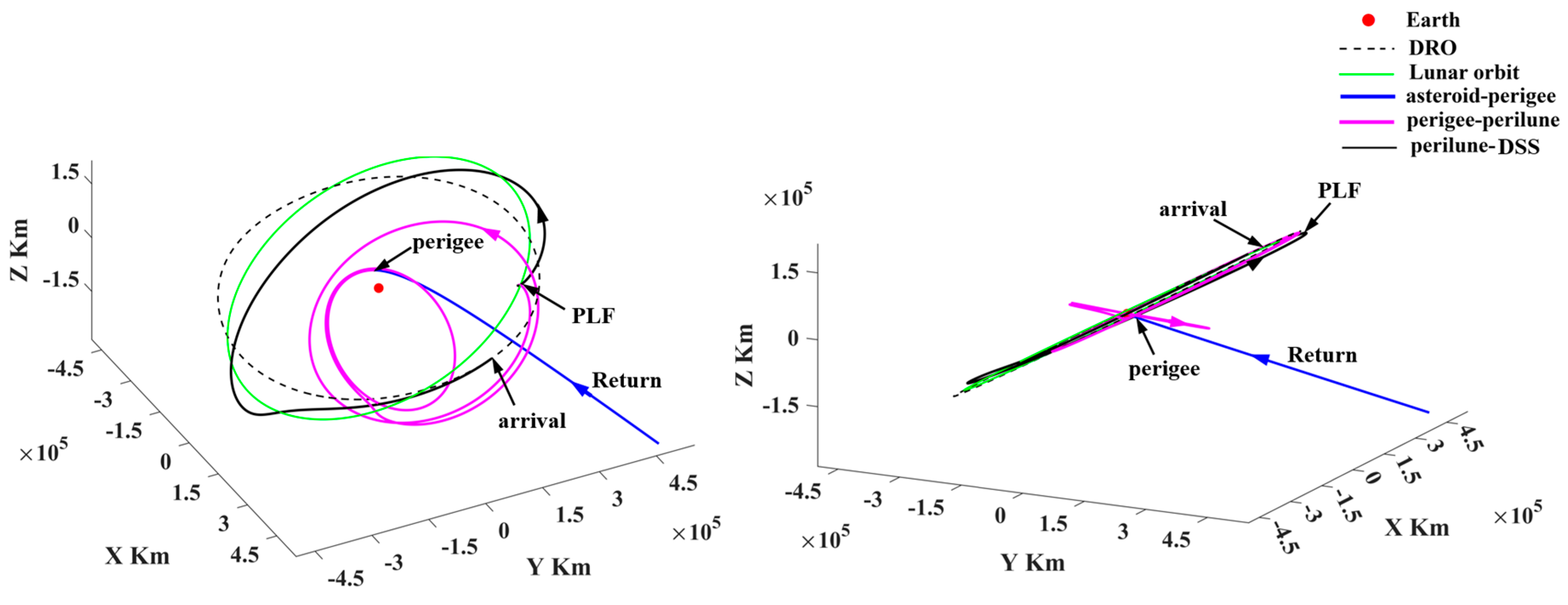
Missions toward PHAs require considerable propellant mass consumption. To solve this problem, the preliminary mission analysis and trajectory optimization in an Earth–PHA transfer have been investigated through the use of propellantless or continuous thrust propulsion systems, such as the study of the solar sail-based Apophis rendezvous mission [15] and the investigation of the potentialities of an electric sail for missions toward PHAs [16]. However, the current asteroid explorations are still expensive and inefficient. Low-cost mission concepts to explore large numbers of PHAs are desired. We proposed a mission scenario involving the reusable probes that explore the PHAs with multiple round trips. It is assumed that a batch of reusable probes depart from and return to a DRO Service Station (DSS) deployed in a distant retrograde orbit (DRO) in cislunar space, where the probes are refueled for reusability. In a single round trip from cislunar space to PHAs, the probe flies by one or more PHAs, as shown in Figure 1. Logically, multiple round trips of reusable probes explore large numbers of PHAs. This concept is inspired by asteroid redirect, reusable probes, and refueling in a DRO. They were separately studied previously and combined in this research. For example, the Earth-Moon transfer orbits based on DRO are investigated [17,18,19] and a lunar-orbiting satellite constellation based on DRO for wireless energy supply is proposed [20]. It is noted that refueling in a DRO has also been proposed [21,22,23,24], including supporting the missions to Mars [25,26].
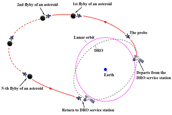
Figure 1.
Schematic diagram of PHA exploration mission (the red, magenta and black lines denote the single round trip, lunar orbit and DRO, respectively).
In order to verify the feasibility of the proposed mission concept, we raised a trajectory design problem released in the 12th edition of China’s Trajectory Optimization Competition on 20 August 2022. It was expected that a total of 20 reusable probes explore as many PHAs as possible with the manner of a close flyby within a 10-year time window from 1 January 2025 to 31 December 2034. The maximum range of the probe relative to Earth was set to 20 million kilometers. The participants were required to design multiple round-trip trajectories of a total of 20 reusable probes to fly by PHAs in a multi-body dynamical environment.
As the authors who proposed the problem, we present our approaches in this article. The remainder of this paper is arranged as follows. Section 2 gives the problem descriptions, including orbital dynamics, mission constraints, and performance indices. Section 3 presents the trajectory analysis, including simplified orbital dynamics and diversified transfer trajectories in cislunar space. Section 4 describes trajectory design, including trajectory database construction, trajectory patching and correcting, and mission allocation. Section 5 presents the trajectory solutions. Finally, conclusions are drawn in Section 6.
2. Problem Descriptions
2.1. Orbital Dynamics
- (1)
- For the reusable probes
The orbital motion for a reusable probe is modeled by a Sun–Earth–Moon–probe restricted four-body problem (SEM-RFBP), and the equation of motion is expressed in the Earth-centered inertial coordinates (ECI).
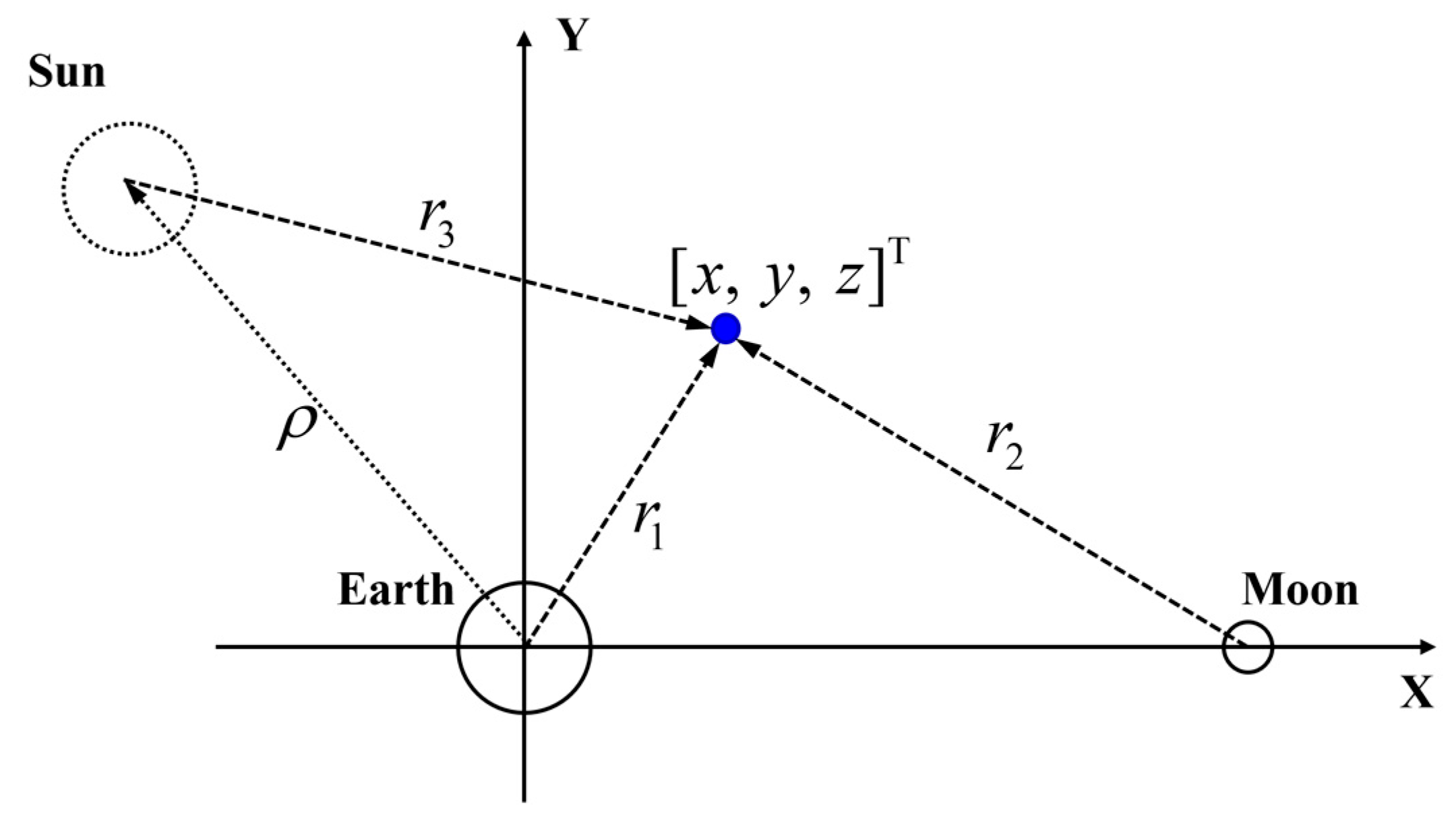
where (=398,600.00 km3/s2), (=4902.80 km3/s2), and (=1.32712440018 × 10¹¹ km3/s2) are the gravitational constants of the Earth, Moon, and Sun, respectively; , , and are the position vectors of the probe, the Moon, and the Sun, respectively. The Moon and the Sun follow geocentric Keplerian orbits referenced in ECI, of which the ephemerides can be found in Appendix A.
The alternative form of Equation (1) can be expressed in Earth–Moon rotating coordinates (ROT), in which the origin is located at the center of the Earth, the x-axis is directed from the Earth to the Moon, the y-axis is in the Earth–Moon orbital plane and perpendicular to the x-axis, and the z-axis completes the right-handed triad. Both the Earth and the Moon are stationary in ROT, and the Moon is located in [1 0 0] if the Earth–Moon distance is set as a dimensionless unit. As a result, Equation (1) is approximated as a set of dimensionless equations expressed in ROT that are given as follows:
where is the Earth–Moon mass ratio; is the normalized mass of the Sun; is the position vector of the Sun in ROT (see Appendix A); and , , and are the distances from the probe to the Earth, Moon, and Sun, respectively, which are expressed as follows:
It is noted that the parameters in Equation (2) and the normalized units are given in Table 1. If , the SEM-RFBP becomes an Earth–Moon circular restricted three-body problem (EM-CRTBP).

Table 1.
The parameters and the normalized units for Equation (2).
- (2)
- For the DSS
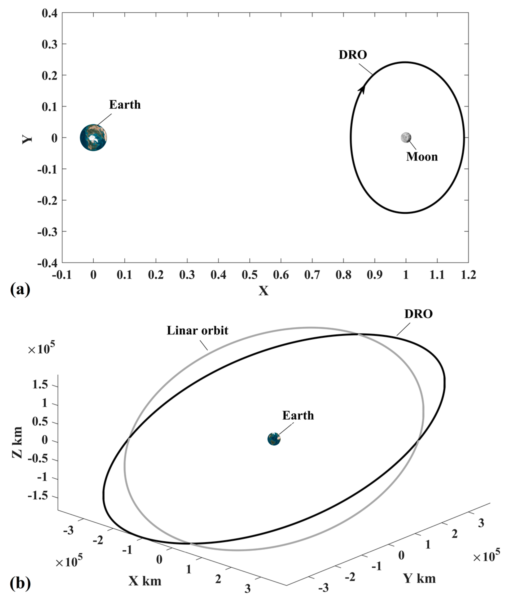
The orbital motion of the DSS is modeled by the EM-CRTBP. Specifically, the DSS is deployed in a DRO, which is a stable periodic orbit around the Moon. The orbit of the DSS expressed in ROT is approximated by Fourier polynomials, and the ephemeris of the DSS is given in Appendix B. The DSS’s orbits in both ROT and ECI are shown in Figure 2.
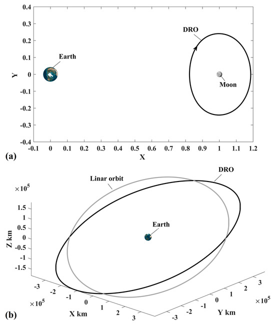
Figure 2.
Schematic diagram of the DRO for deploying the DSS ((a) in ROT and (b) in ECI).
- (3)
- For the PHAs
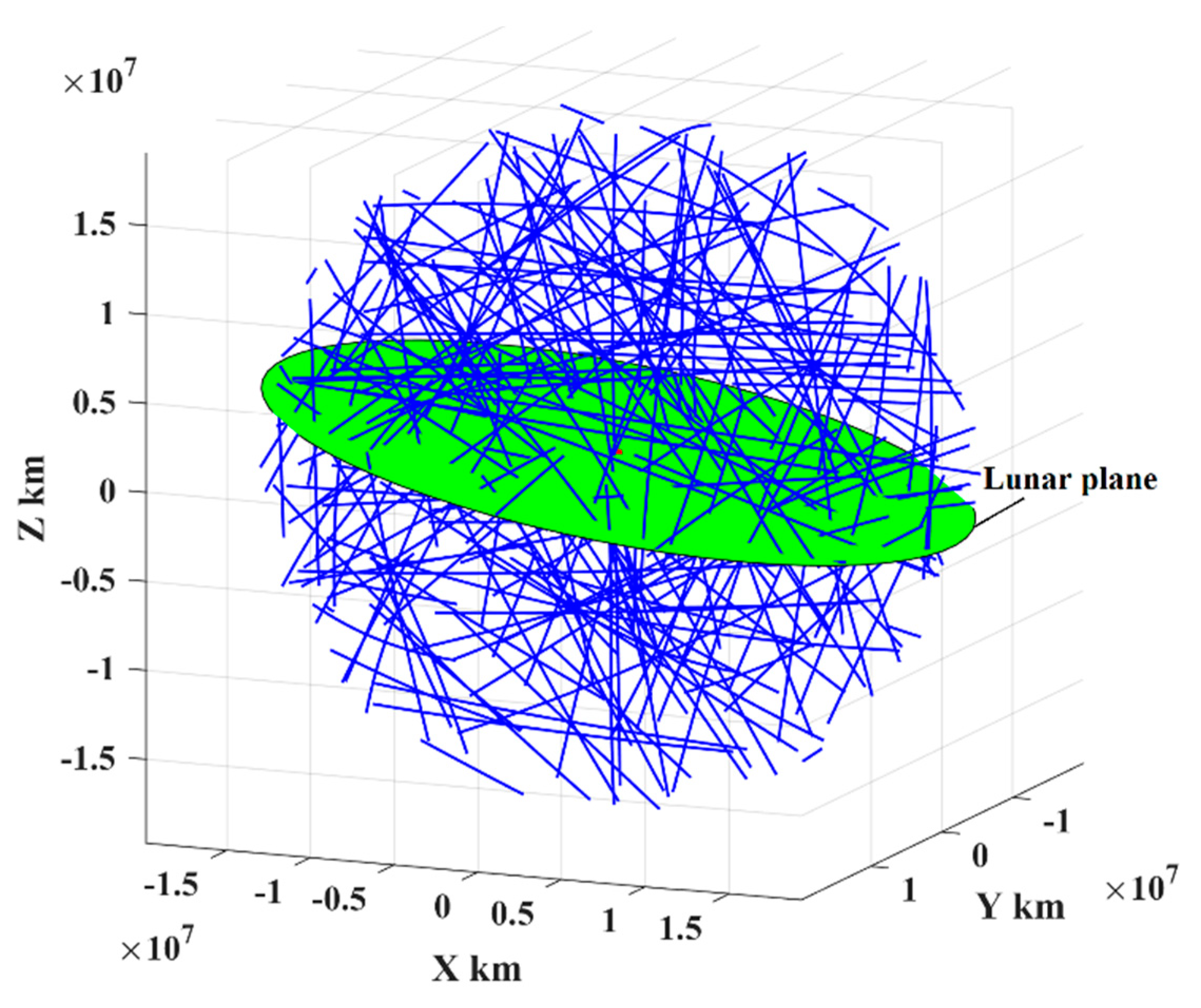
The PHAs in this study are referred to as those that reach inside the sphere with a radius of 20 million kilometers relative to Earth. The orbital motion of the PHAs is assumed to follow the heliocentric two-body orbital dynamics. We selected a total of 167 PHAs with diameters no less than 100 m as the representative targets. As shown in Figure 3, the part trajectories of these PHAs denoted by blue lines are nearly straight inside the proposed sphere.
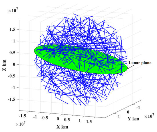
Figure 3.
The part trajectories of the PHAs inside the sphere with a radius of 20 million kilometers.
2.2. Mission Constraints
The trajectory design is subject to a series of mission constraints that intentionally consider technological feasibility, which are listed as follows:
1: The probe explores PHAs.
(1-a): The round-trip exploration missions of all the probes should be completed between MJD 60676 (1 January 2025) and MJD 64328 (31 December 2034).
(1-b): The probe must implement a close approach to a PHA with a distance less than 10 km, which is then considered a valid exploration of a PHA, and the small body gravity is neglected.
(1-c): The orbital radius of the probes should be greater than 6578 km (or 200 km in orbital altitude) and less than 20 million km from the Earth.
2: The probe returns for refueling.
(2-a): After exploring PHAs, the probe is required to return to the cislunar space. The position and velocity vectors of the probe must match those of the DSS.
(2-b): It takes at least 10 days to complete refueling in the DSS, and there is no limit to the number of probes that can be refueled at the same time.
(2-c): The time of flight (TOF) for each round trip must be less than 4 years.
3: The maneuver capability of the probes
(3-a): The total ΔV executed by a probe for a single round trip should not be more than 2.0 km/s.
(3-b): An orbital maneuver is simplified to an instant velocity impulse, of which the direction is unlimited. The time interval between two successive orbital maneuvers should not be less than 1 day.
2.3. Performance Indices
The trajectory design results are evaluated based on three performance indices. The first performance index is given as
where N is the total number of PHAs explored in all exploration missions, and is the integer part of x. The second performance index is given as
where M is the number of the used probes. The third performance index is given as
where is the total velocity increments executed by the ith probe (including all exploration missions). The team with the largest J1 wins; when J1 scores are equal, the team with the lowest J2 wins; and in the case that J1 and J2 have the same score, the team with the lowest J3 wins.
3. Trajectory Analysis
A single probe round trip to explore PHAs from the DSS can be straightforwardly divided into three segments: (1) the escape trajectory from the DSS and cislunar space, (2) the interplanetary Earth–PHA–Earth trajectory, and (3) the capture trajectory to cislunar space and the DSS. These three segments are further classified into two categories considering the primary gravitations acting on the probe: the heliocentric two-body interplanetary trajectory (segment 2) and the multi-body dynamics trajectories in cislunar space (segments 1 and 3). The former involves the proper PHAs flyby sequence, and the latter concerns the rational use of lunar and solar gravity assists, such as the powered lunar flyby (PLF, a tangential velocity impulse imposed at the perilune) and weak stability boundary (WSB) to obtain low-energy transfer trajectories [27,28]. In this section, the trajectory segment 1 in cislunar space is analyzed, and segment 3 is deemed to follow the same trajectory mechanics in backward time.
3.1. Simplified Orbital Dynamics
It is necessary to use simplified orbital dynamics to approximate Equations (1) and (2) for trajectory analysis. In this section, the two-body patched conics and the bicircular planar four-body dynamics are introduced, which are used in the following Section 3.2 and Section 3.3.
- (1)
- The two-body patched conics
The trajectories in the multi-body gravitational field can be simply patched by the two-body conics in ECI, MCI, and HCI, in which the Earth, the Moon, and the Sun are considered as the primary bodies, respectively. In the sphere of influence of the gravitational body, the probe trajectory follows the Keplerian orbital dynamics and the equation of orbital energy:
where E is orbital energy; r and v are the orbital radius and velocity of the probe, respectively; is the gravitational constant of the gravitational body; and is the desired escape velocity at the sphere of influence (SOI). The two-body patched conics provide a simple analysis technique for escape or capture of the Earth and the Moon.
- (2)
- The planar bicircular restricted four-body dynamics
The planar bicircular restricted four-body problem (PBRFBP) is a simplification of Equations (1) and (2). In this case, the Sun is assumed to revolve in a circular orbit with an angular velocity ( 1/TU) around the Earth with the orbital radius ( DU), as shown in Figure 4. Therefore, the position vector of the Sun is expressed as
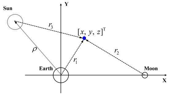
Figure 4.
The diagram of the PBRFBD.
The equations of motion of PBRFBP are given as follows:
where is the phase of the Sun at , and is expressed as follows:
Unlike Equation (2), Equation (9) is decoupled with the ephemerides of the Sun and the Moon and then is more concise for the analysis of the trajectories reaching the perilune and the perigee from the DRO, which includes the analysis of the low-energy transfer trajectories with the WSB ballistic arcs (see Section 3.3 for details).
3.2. Analysis of Orbital Energy for Escape from the Cislunar Space
There are three typical strategies for a probe to escape the cislunar space (or escape the gravitational field of the Earth): direct escape, perigee escape, and perilune escape. These strategies are referred to as exerting an escape maneuver (a velocity increment) at three featured states: the DRO perigee, the perilune, and the perigee. For the latter two cases, it is assumed that the probe leaves the DRO to reach the perilune or the perigee.
- 1.
- Direct escape
Based on Equation (7), the orbital energy of the DSS in ECI is computed using the orbital states of the DRO perigee (given in Appendix B) with and , which is given by
Given a desired escape velocity , the velocity increment is simply computed as
- 2.
- Perigee escape
Assuming that the probe departs from the DSS and reaches the perigee with ( is the Earth’s radius), its velocity at the perigee can be computed as follows:
where is given in Equation (11). Given a desired escape velocity , the velocity increment is simply computed as
- 3.
- Perilune escape
First, assuming that the probe departs from the DSS and reaches the perilune with ( is the Moon’s radius), its velocity at the perilune referenced in MCI can be computed as follows:
where and are the orbital states of the DRO perilune in MCI, which can be derived by the ephemeris of the DSS in Appendix B.
Moreover, assuming that the probe departs from the Earth’s SOI with a desired escape velocity and reaches the Moon in the same direction as the lunar velocity, its velocity relative to the Moon is expressed by
where and are the lunar orbital radius and velocity, which can be derived from the lunar ephemeris in Appendix A. Then, based on the two-body patched conics, the velocity increment is simply computed as
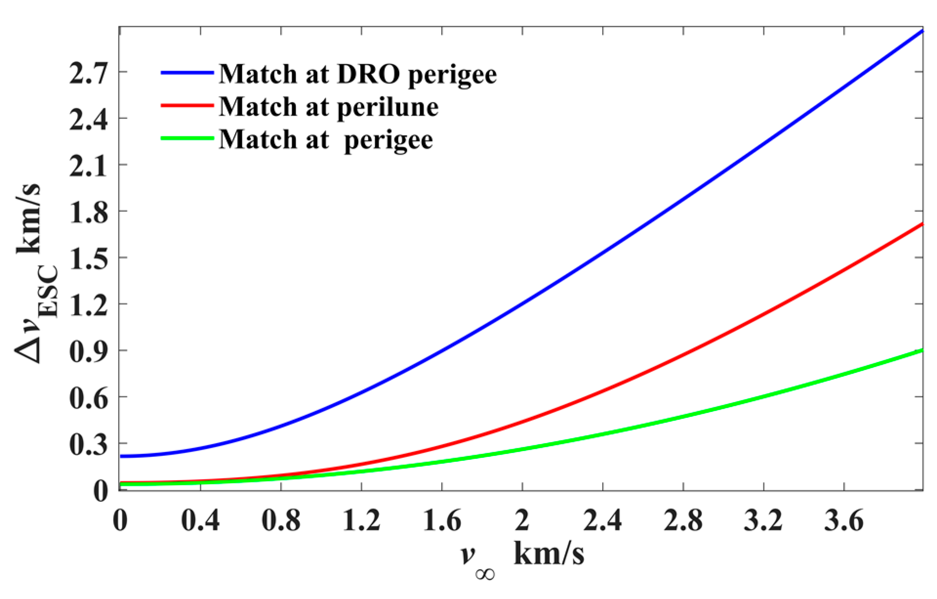
Consequently, the lower bound of the required velocity increment (denoted as ) at the three featured states with respect to is computed straightforwardly, as shown in Figure 5. It is noted that the exerted at the perigee to match is much lower than those exerted at the other two featured states, and therefore, the case with the escape maneuver at the perigee is considered in the following trajectory design.
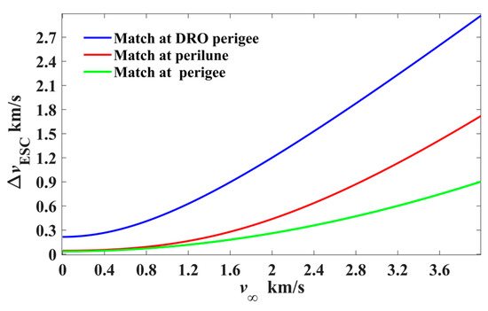
Figure 5.
The velocity increment with respect to the desired escape velocity (exerted at three featured states).
3.3. Analysis of Trajectories Reaching the Perilune and the Perigee from the DRO
First, let us consider the gravitational forces of the Earth and the Moon only; the trajectories from the DSS to the perigee/perilune in EM-CRTBP ( in Equation (2)) can be categorized as in the following three cases (as shown in Figure 6):
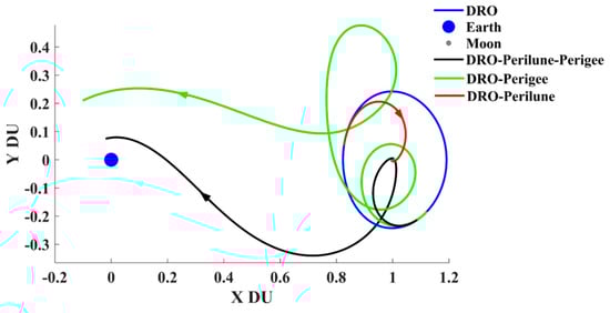
Figure 6.
The probe arrivals at the perigee/perilune from DRO (in ROT).
Case 1: The probe departs from the DRO with a velocity impulse and arrives at the perilune.
Case 2: The probe departs from the DRO with a velocity impulse and arrives at the perigee.
Case 3: The probe departs from the DRO with a velocity impulse to the perilune first, and then arrives at the perigee after making use of a PLF.
For these three cases, we analyzed the probe trajectories departing from the DRO to the perilune and the perigee with a total velocity increment of no more than 200 m/s.
- (1)
- Case 1
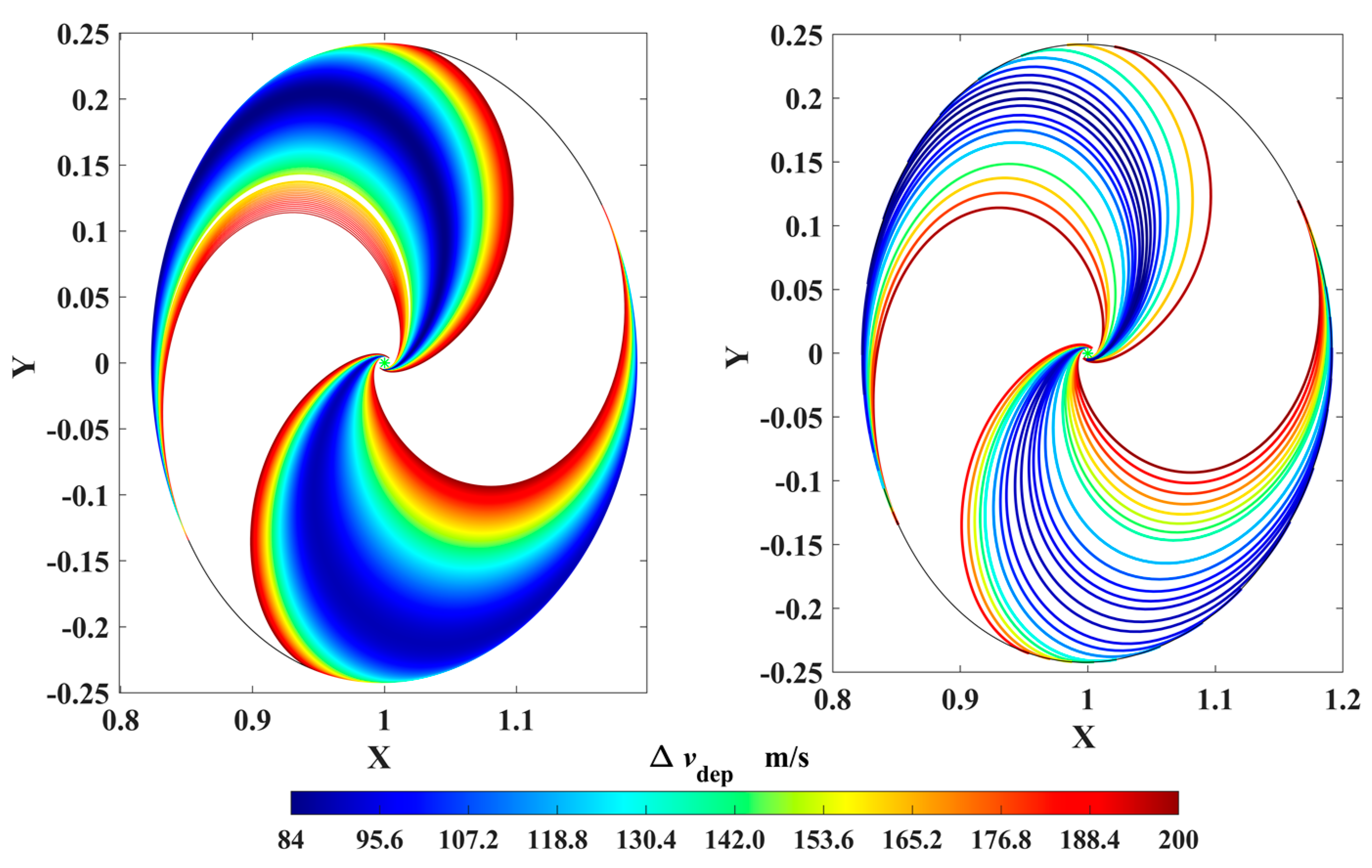
Considering that the DRO is a retrograde orbit around the Moon, the simplest and most efficient strategy to rapidly escape from the DRO to a perilune is exerting an opposite impulse velocity on the probe; then the probe approaches the Moon. The transfer trajectories by which the probes reach perilune with an orbital altitude of 200 km are shown in Figure 7, where the color bar represents the velocity impulse magnitudes, and the minimum is 84 m/s. The departure positions shown in Figure 8 are concentrated in two areas, and their corresponding arrival perilunes are distributed in the regions in front of and behind the Moon. Both Figure 7 and Figure 8 indicate that the probe is able to reach the low-altitude perilune with a small velocity impulse, which provides the opportunities to utilize lunar gravity assist.
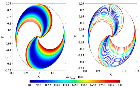
Figure 7.
The probe trajectories departing from the DRO and arriving at the perilune (in ROT).
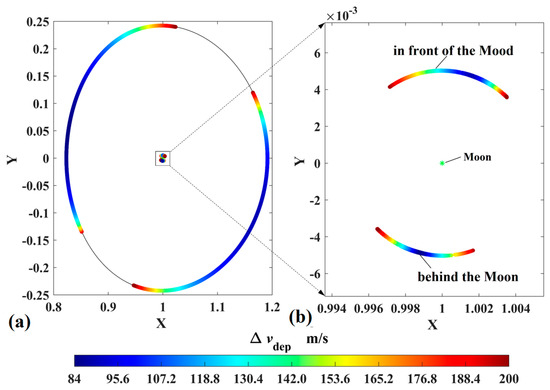
Figure 8.
The orbital positions of the DRO departure and the perilune arrival (in ROT, (a) the departure positions and (b) the corresponding arrival perilunes).
- (2)
- Case 2
Similarly, the strategy for reaching a low-altitude perigee is exerting a velocity impulse (also no more than 200 m/s) in the opposite direction on the DRO to decrease orbital energy. Let the TOFs be no more than 30 days; it is found that six types of transfers can reach the perigees inside the Earth’s sphere of 70,000 km, as shown in Figure 9. In this case, the minimum velocity impulse is 47 m/s, and the minimum perigee altitude is 51,339 km. However, these results show that the perigee’s altitudes are still high. To further reduce the perigee’s altitude, the transfer trajectories in case 3 that use a PLF are introduced.
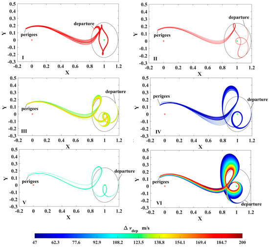
Figure 9.
The direct transfer trajectories leaving the DRO to the perigees with a velocity impulse (in ROT, the red and green asterisks denote Earth and Moon, respectively).
- (3)
- Case 3
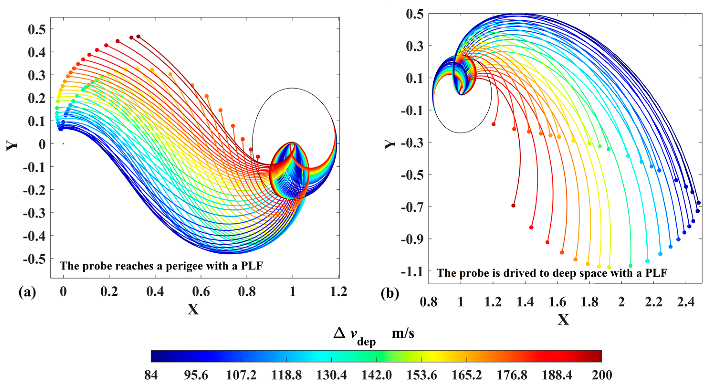
The transfer trajectory in case 3 is the expansion of the transfer trajectory in cases 1 and 2: a PLF is added to drive the probe to low-altitude perigees. Based on the trajectories in Figure 7, the transfer trajectories are shown in Figure 10, where the perilune impulse is in the direction of orbital velocity, and its magnitude is set to ensure the total velocity impulses are 200 m/s. In Figure 10, it can be found that the PLF decreases the orbital energy and drives the probe to a perigee (the minimum altitude is 17,936 km, as shown in Figure 10a) or increases the orbital energy and drives the probe to deep space (as shown in Figure 10b). Therefore, the PLF is considered an effective means to significantly change the orbital energy.
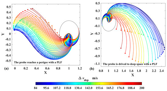
Figure 10.
The transfer trajectories leaving the DRO to the perigees with a PLF (in ROT).
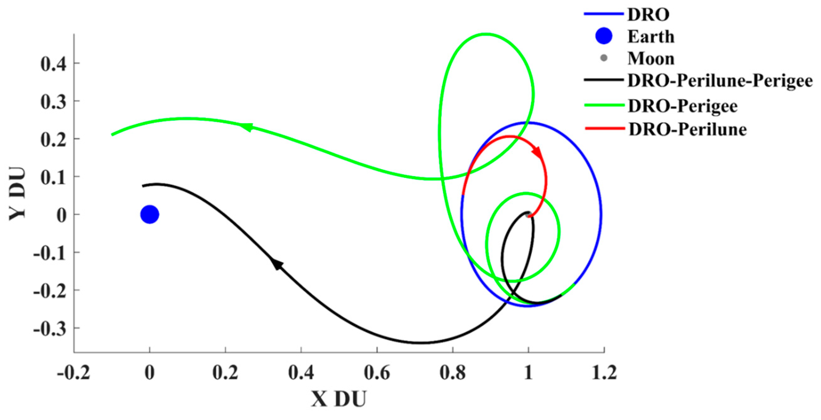
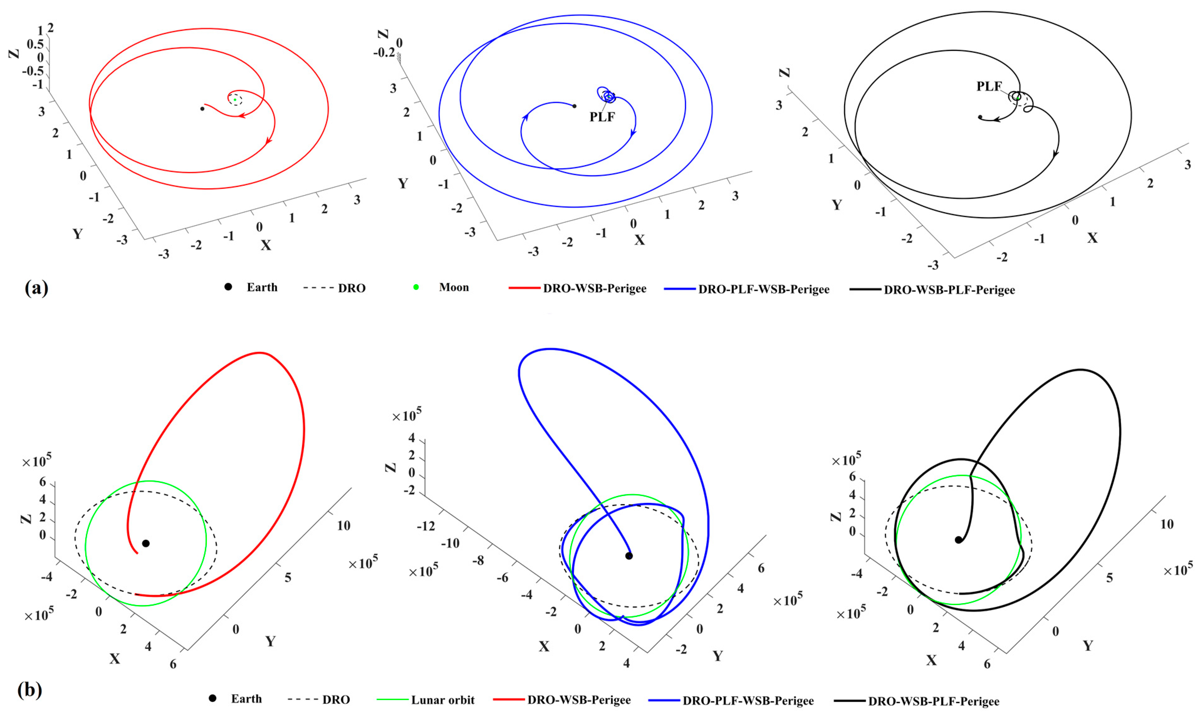
Second, if the probe moves outside the cislunar space in which the solar gravitation is considered (using PBRFBP in Equation (9)), the probe can use a WSB ballistic arc to approach the low-altitude perigees. By using this approach, the orbital energy is changed under the influence of solar gravitation [29]. Meanwhile, it can also help to find varied departure (or arrived) velocity vectors relative to the DRO [29]. As shown in Figure 11, three cases of trajectories departing from the DRO to a perigee with a WSB ballistic arc are taken as examples:
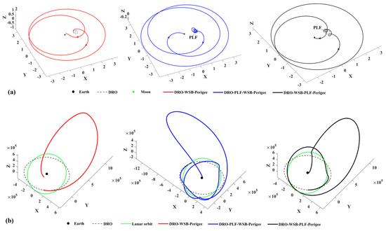
Figure 11.
The trajectories leaving the DRO to the perigee with WSB ballistic arcs and PLFs ((a) in ROT and (b) in ECI).
Case 1: The probe directly arrives at the perigee after it uses a WSB ballistic arc, as the red orbit shows in Figure 11a,b.
Case 2: The probe first reaches the perilune and uses a PLF to approach a WSB ballistic arc, then it arrives at the perigee finally, as the blue orbit shows in Figure 11a,b.
Case 3: The probe first uses a WSB ballistic arc to adjust the trajectory and then reach the Moon. Later, a PLF drives the probe to arrive at the perigee, as the black orbit shows in Figure 11a,b.
In Figure 11, case 1 uses the WSB ballistic arc only, while case 2 and case 3 use both PLF and WSB ballistic arcs. It is found that the probe can reach a low-altitude perigee especially when both PLF and WSB ballistic arcs are utilized. Furthermore, the orbital inclination of the orbital estates at each perigee is increased in case 2, and the orbit is retrograde in case 3. Therefore, the combination of PLF and WSB is considered an attractive means to change the orbital altitude and inclination to match a wide range of escape velocity , at the expense of longer TOFs. In this study, case 2 and case 3 are used to find more various low-energy escape/capture orbits, both of which follow a DSS−perilune−perigee flight sequence.
4. Trajectory Design
In terms of the analysis given in the previous section, the trajectory design strategy is then proposed. First, we construct two trajectory databases, one for trajectory segments of Earth–PHAs–Earth and the other for those of DSS−perilune−perigee for escape and perigee−perilune−DSS for capture. Next, the trajectory segments in these databases are patched to form a series of round-trip trajectories. Finally, the trajectory solutions are obtained by allocating round-trip trajectories to the reusable probes.
4.1. Constructing Earth–PHAs–Earth Interplanetary Trajectories Database
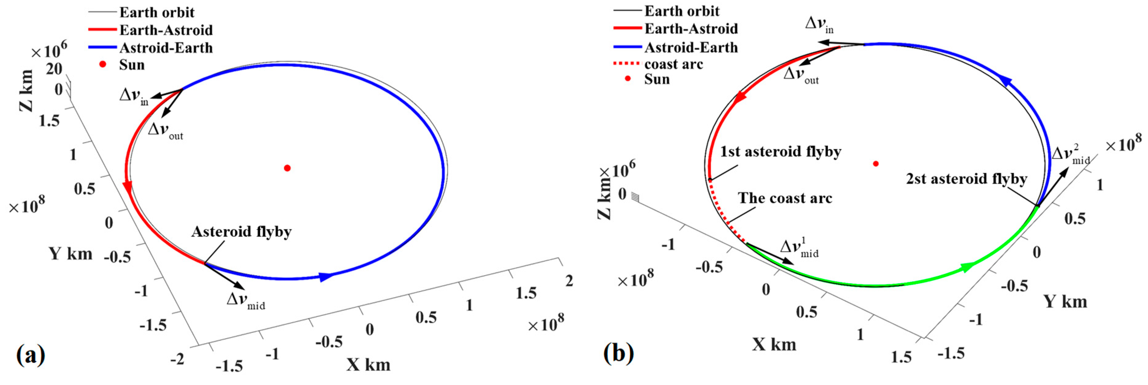
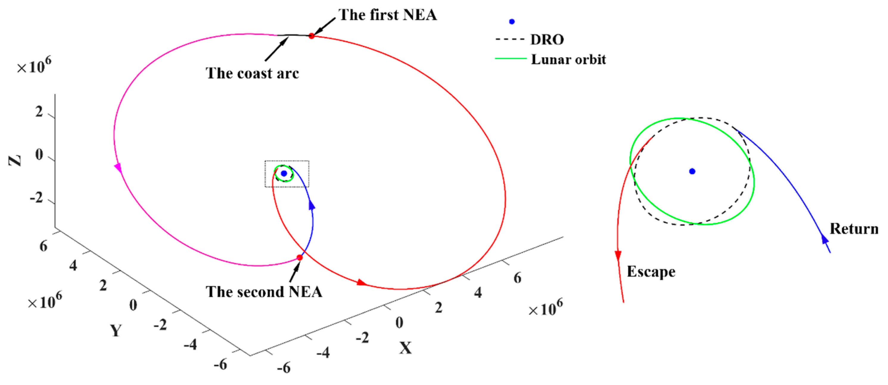
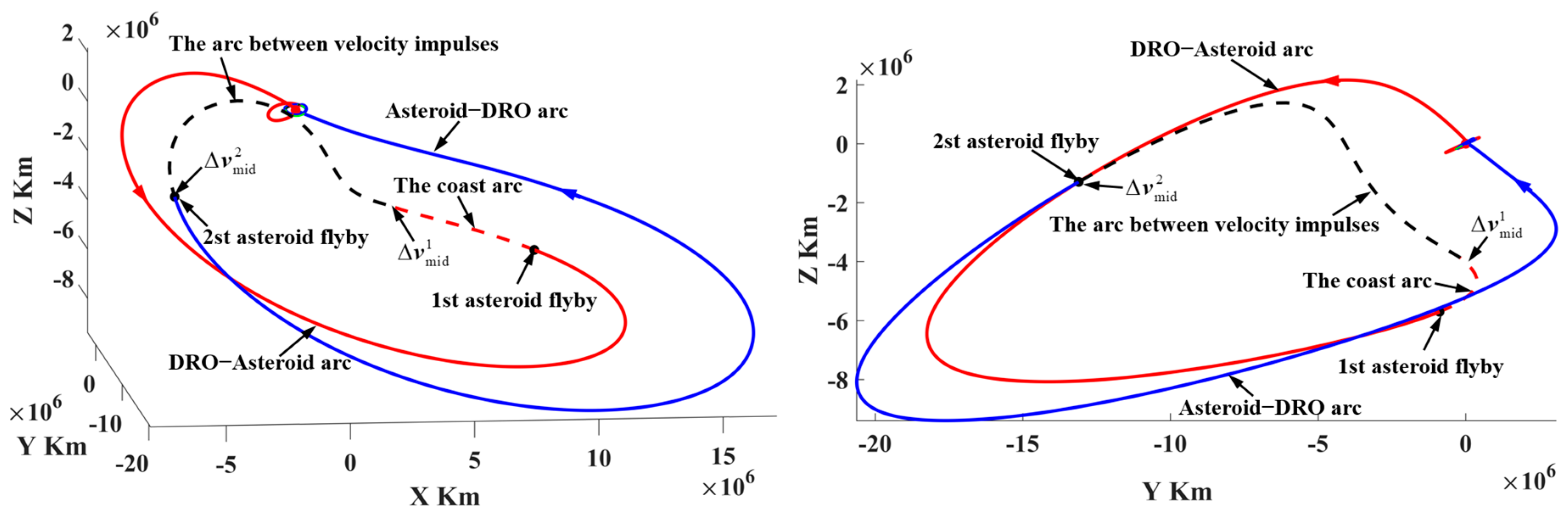
For simplicity, the interplanetary trajectories with one and two PHAs explored are considered, which have the sequence of Earth–PHA–Earth and Earth–PHA–PHA–Earth, respectively, as shown in Figure 12. In Figure 12a, the probe with one PHA explored departs with to fly by a PHA, exerts to return, and is captured with . In Figure 12b, the probe with two PHAs explored departs with to fly by the first PHA, then coasts and exerts to reach the second PHA, exerts to return, and then is captured with . The interplanetary trajectories are approximately modeled by heliocentric two-body orbital dynamics. Therefore, the trajectory in Figure 12a with is computed by solving two Lambert problems (Earth–PHA and PHA–Earth orbits), and the trajectory in Figure 12b with and is obtained by solving three Lambert problems.

Figure 12.
The transfer trajectories of Earth–PHAs–Earth ((a) Earth–PHA–Earth and (b) Earth–PHA–PHA–Earth).
First, for the case in Figure 12a, an optimization problem with an objective and three variables is proposed as follows:
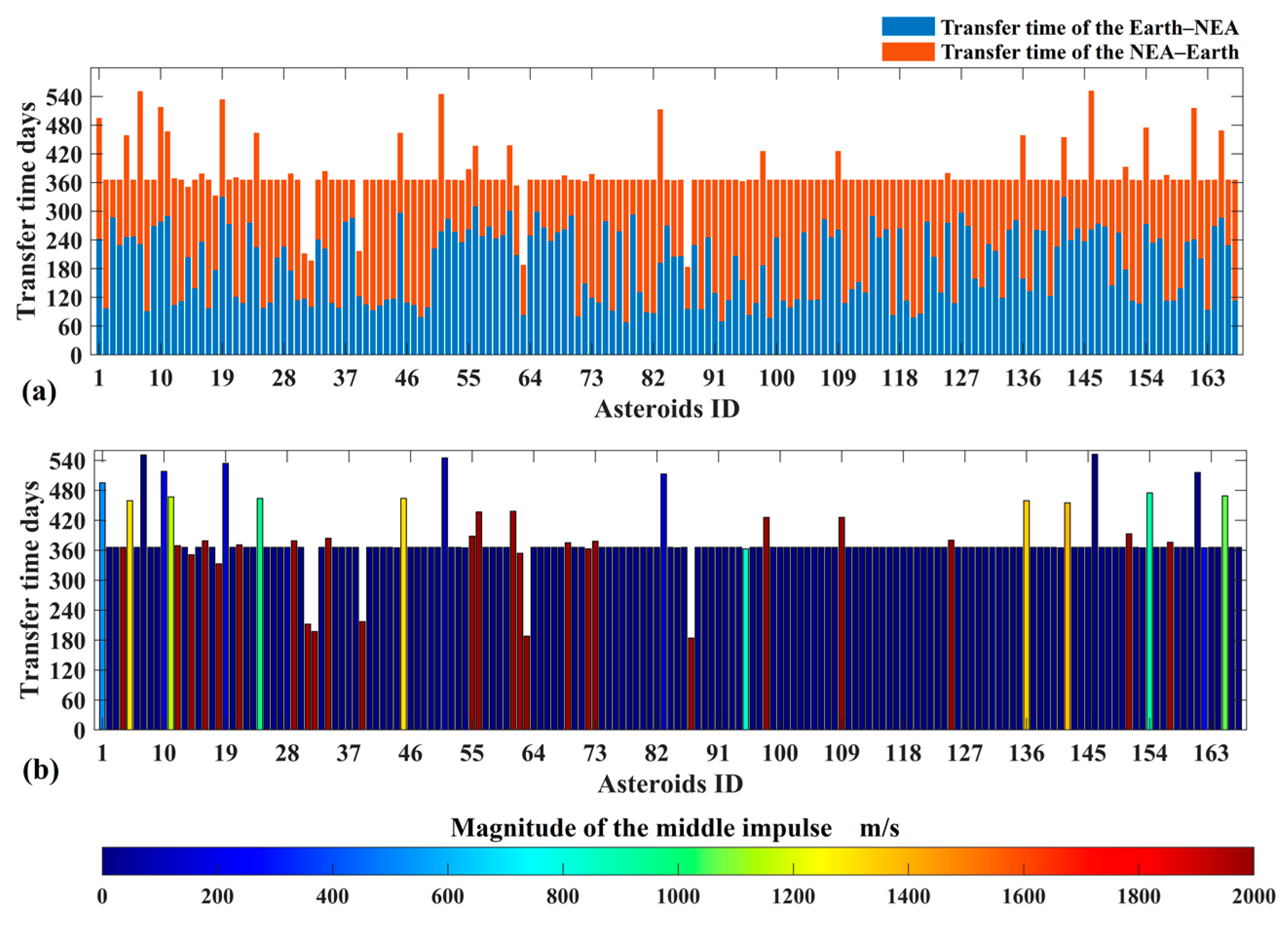
where and are the TOFs of the Earth–PHA and PHA–Earth trajectory segments, respectively; is the moment at the PHA’s flyby; and the upper and lower bounds of given by and are the times of the PHA’s entry into and exit from the Earth’s sphere with a radius of 20 million kilometers. By solving the optimization problem using a genetic algorithm, the Earth–PHA–Earth transfer solutions with the minimum for the 167 PHAs are computed, as shown in Figure 13. In Figure 13a, and are denoted by the blue and red bars, respectively. It can be found that the TOFs are concentrated in the value of 366 days, which implies that most interplanetary trajectories have the same flight times as the Earth’s orbital period. The color bars in Figure 13b denote the magnitude of , which implies that is small if the flight time is 366 days.
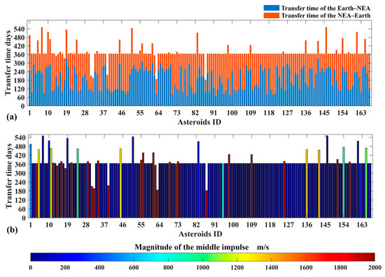
Figure 13.
The transfer time and minimum magnitude of the middle impulse of Earth–PHA–Earth trajectories ((a) and are denoted by the blue and red bars, respectively, (b) the color bar denote the magnitude of ).
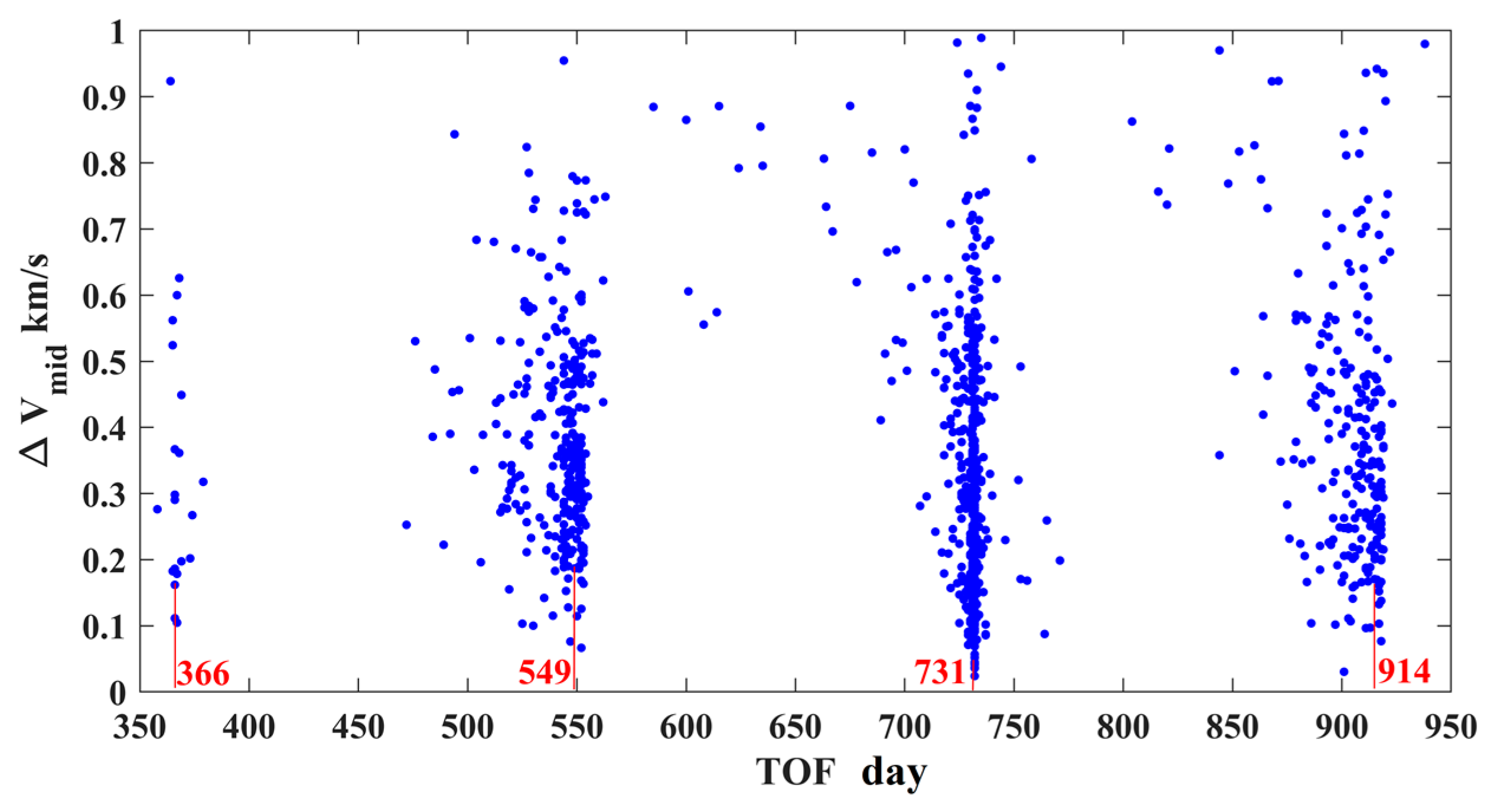
Second, for the case in Figure 12b, the positions of the two PHAs’ flybys are regarded as the two intermediate nodes in the trajectory with the sequence Earth–PHA–PHA–Earth. Similarly, an optimization problem with an objective and five variables is proposed as follows:
where and are the TOFs of the Earth–PHA and PHA–Earth trajectory segments, respectively; is the TOF of the coast arc; and and are the moments when the probe flies over the first and the second PHA, respectively. The upper and lower bounds of and are the moments of the PHA’s entries into and exits from the Earth’s sphere, respectively. Finally, a total of 1029 interplanetary trajectories with no more than 1 km/s are obtained, of which the -TOF is shown in Figure 14. It is found that the solutions are concentrated in four regions, of which the TOFs are grouped into 366, 549, 731, and 914 days, respectively. These TOFs demonstrate that the interplanetary trajectories are resonant with respect to the Earth.
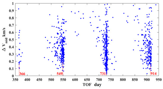
Figure 14.
The -TOF map of Earth–PHA–PHA–Earth trajectories (the TOFs are grouped into 366, 549, 731, and 914 days, respectively).
4.2. Constructing DSS−Perilune−Perigee Trajectory Database
The escape trajectory from the DSS to the perigee that matches the interplanetary trajectory is proposed as follows: the probe departs from the DSS, reaches a perilune with a PLF, and then reaches a low-altitude perigee. The DSS−perilune−perigee trajectories modeled by Equation (2) are computed by using a global search method introduced by Ref. [29], which includes two steps: parameterization of the velocity impulses and database construction by a Monte Carlo trajectory shooting method. In this study, the PLF is an essential means to obtain transfer trajectories, but the transfer trajectories may or may not utilize the WSB ballistic arcs.
Suppose that the orbital state of the probe on the DSS is at the time of departure ; a velocity impulse is exerted, and it is expressed as
where is the magnitude of ; and are the azimuth and elevation angles representing the direction of in a coordinate frame (), of which the origin is the DSS; is aligned with ; points along the direction normal to the DRO orbital plane; and completes the right-handed triad. When the probe reaches the perilune, a tangential velocity impulse with a magnitude of is exerted. The trajectory of the probe from the DSS to the perigee can be obtained by numerical integration with five parameters , , , , and ), which are given in Table 2 and randomly sampled to propagate the corresponding trajectories. In addition, the orbital radius of the perigee and the perilune are empirically set to be no more than 50,000 km and 5000 km, respectively, and the TOFs of the DSS–perilune and perilune–perigee trajectory segments are both set to be no more than 100 days.
Table 2.
Parameter list for the Monte Carlo trajectory shooting process.
As a result, a total of 23,255,437 perigees (or trajectory samples) are generated to construct the DSS−perilune−perigee trajectory segment database. The ΔV-TOF map of these trajectory segments is shown in Figure 15 ( in this case), where the red dots represent the Pareto front. Moreover, the perigee–perilune–DSS trajectory database (designed in backward time) can be constructed by using the same method, which is not presented for conciseness. It is noted that we used a CPU workstation equipped with 64 cores (CPU: AMD Ryzen Threadripper PRO 5995WX 64-Cores, 2.70 GHz), and the computational time was about six hours to construct the DSS–perilune–perigee trajectory segment database.
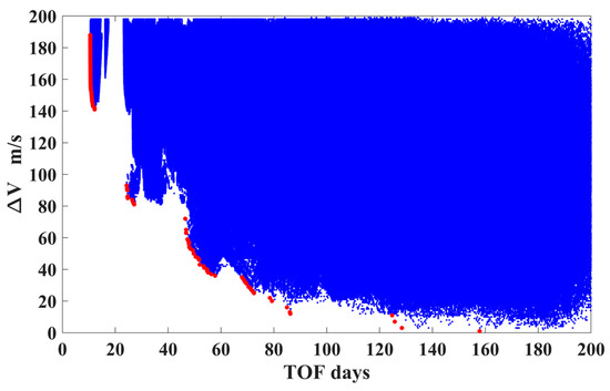
Figure 15.
The ΔV-TOF map of the computed DSS−perilune−perigee trajectories (the red dots represent the Pareto front).
4.3. Generating Round-Trip Trajectories
Generating round-trip trajectories is referred to as patching the interplanetary trajectories and the DSS–perilune–perigee/perigee–perilune–DSS trajectory segment. The first step is coarse patching in terms of the classical B-plane technique, and the second step is refined patching to be subject to the orbital dynamics and mission constraints given in Section 2.1 and Section 2.2.
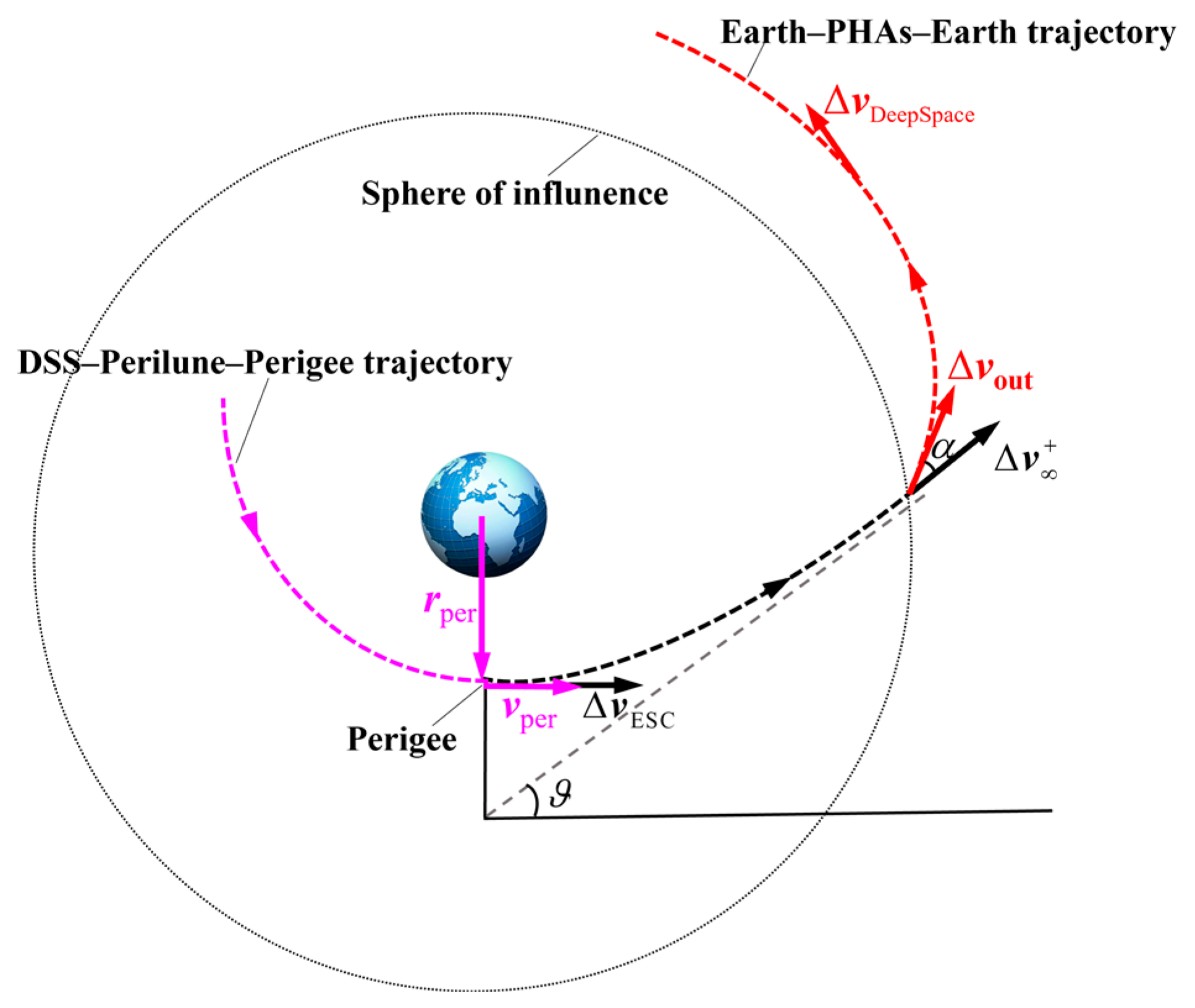
Based on the two-body patched conics approximation, the coarse patching is to match the orbital states of the probe at the perigee in the DSS−perilune−perigee database and the departure velocity impulses in the Earth−PHAs−Earth interplanetary trajectory database. As shown in Figure 16, is a virtual quantity that is computed by the orbital state at the perigee, and the patched trajectory can be approximated as a powered Earth’s gravity assist, which is used to compute the velocity impulse at the perigee. The velocity increment is imposed to increase the orbital energy and drives the probe into a hyperbolic orbit.
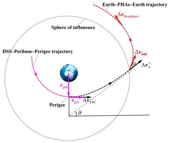
Figure 16.
Illustration of patching the Earth−PHAs−Earth trajectory and the DSS–perilune–perigee trajectory.
The states at the perigee ([,]) and are patched if the following conditions are satisfied:
where
and is the difference between the time at the perigee and the departure time in interplanetary trajectories. and , which are in terms of (, , ), are computed as follows.
Assuming that the position and velocity vectors at the perigee are denoted by and , respectively, the velocity vector becomes () after the velocity increment is imposed at the perigee. Based on the orbital energy in Equation (7), if , the is given by
then
After the escape, the direction of the probe velocity vector rotates an angle (see Figure 16), which is expressed as
Then, the escape velocity is computed as follows:
where
The second step is to minimize the total velocity impulses and refine the trajectory using the orbital dynamics in Equation (1). An optimization problem with an objective and two variables is proposed as follows:
where is the position errors at the patched point (near the Earth’s SOI), and is the velocity impulse in the deep space (e.g., or in Figure 12).
Finally, a total of 1224 precise round-trip trajectories are generated. The first and the second steps make use of a GPU workstation equipped with 4608 cores (GPU: NVIDIA TITAN RTX with a frequency of 1770 MHz and 24 GB frame Buffer) and a CPU workstation (see Section 4.2) and take 1.5 and 0.5 h for computation, respectively.
4.4. Allocating Round-Trip Trajectories
Allocating round-trip trajectories is referred to as selecting a part of 1224 precise round-trip trajectories and allocating them to the 20 probes, while the number of explored PHAs is maximized, and the mission constraints are all satisfied. In fact, this is a straightforward combinatorial optimization problem. First, the chains of round-trip trajectories are constructed, which include one, two, three, or four round trips in sequence. In this way, a total of 335,515 round-trip trajectories chains are constructed in terms of the 1224 round-trip trajectories. The second step is to allocate the 335,515 round-trip trajectory chains to the 20 probes to maximize the number of explored PHAs, in which there are selections. A Monte Carlo method (large-scale random selection) is used to allocate these round-trip trajectories. Both the first and second steps require substantial computational loads. We used the GPU workstation (see Section 4.3), and it took about 1 h to obtain the trajectory solution presented in Section 5.1.
5. Trajectory Solutions
5.1. Solutions Designed in This Study and Submitted in the Competition
In this study, we finally obtained a trajectory solution with J1 = 105, J2 = 20, and J3 = 0.8295 m/s, showing a significant enhancement compared with those submitted in the competition (see Table 3). It is composed of a total of 62 round-trip trajectories (round trips), as presented in Table 4. The time intervals of the 62 round trips, ΔV-TOF map, and PHA flyby positions are shown in Figure 17, Figure 18 and Figure 19, respectively. In the designed results, there are several probes (Nos. 1, 2, 3, 5, and 6; see Figure 17 and Table 4) that explore eight PHAs with four round trips. As for the ΔV-TOF map, there exists a wide range of ΔV-TOF combinations (see Figure 18). Also, there are many PHA flyby positions away from the lunar orbital plane (see Figure 19).
Table 3.
The trajectory solutions submitted by the top five teams.
Table 4.
The trajectory solution with J1 = 105, J2 = 20, and J3 = 0.8295 m/s.
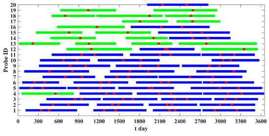
Figure 17.
The time intervals of the 62 round trips (those with one and two PHAs explored are denoted by the green and blue lines, respectively, and the red dots denote the times of flybys).

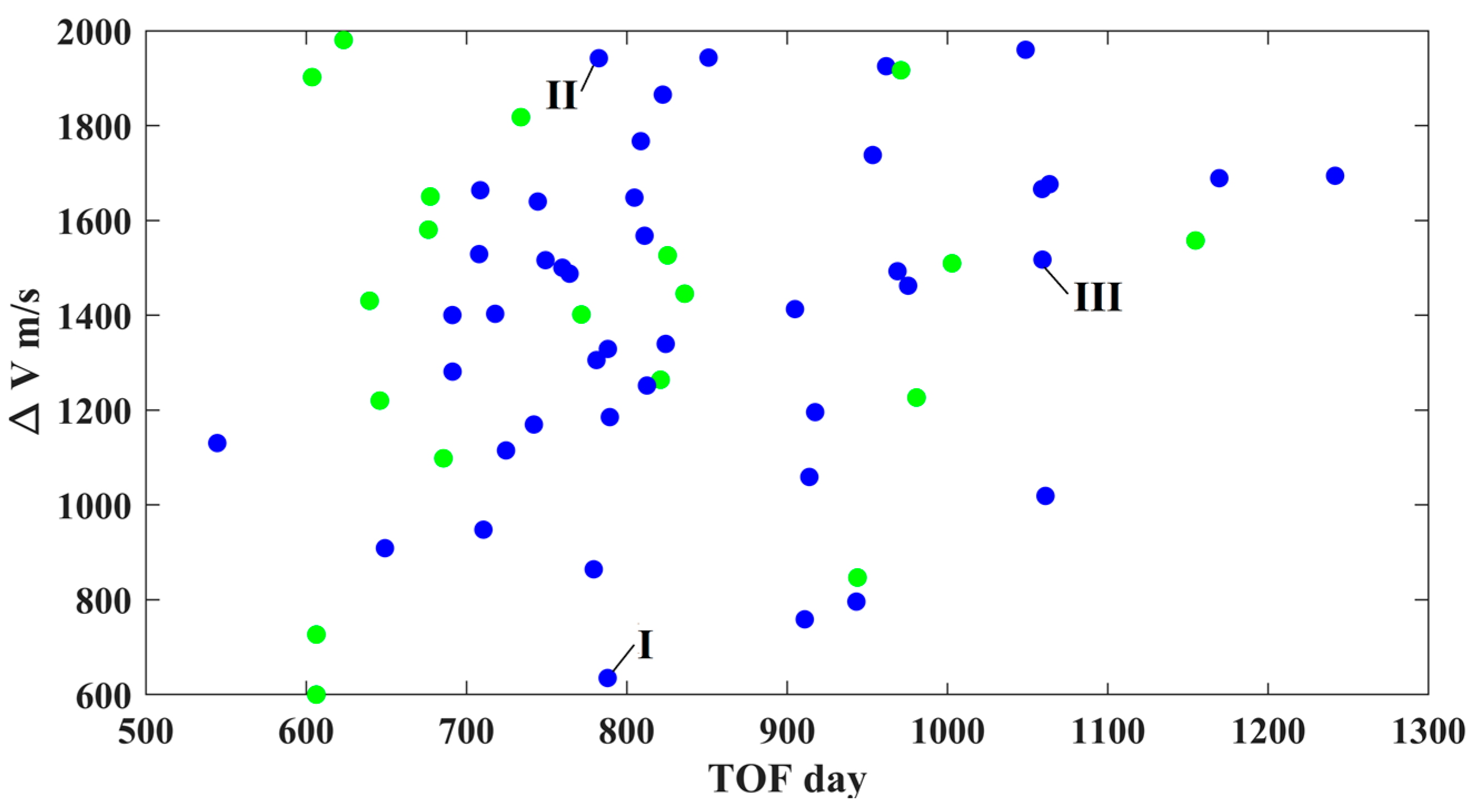
Figure 18.
The ΔV-TOF map of the 62 round trips (those with one and two PHAs explored are denoted by the green and blue dots, respectively; the solutions labeled by I, II, and III are presented in Section 5.2).
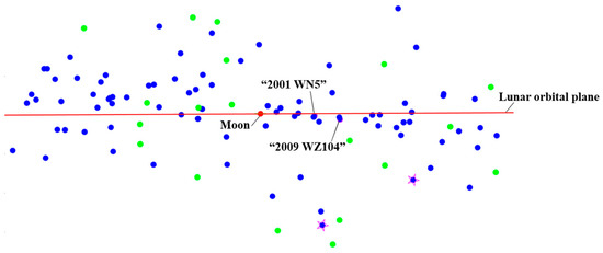
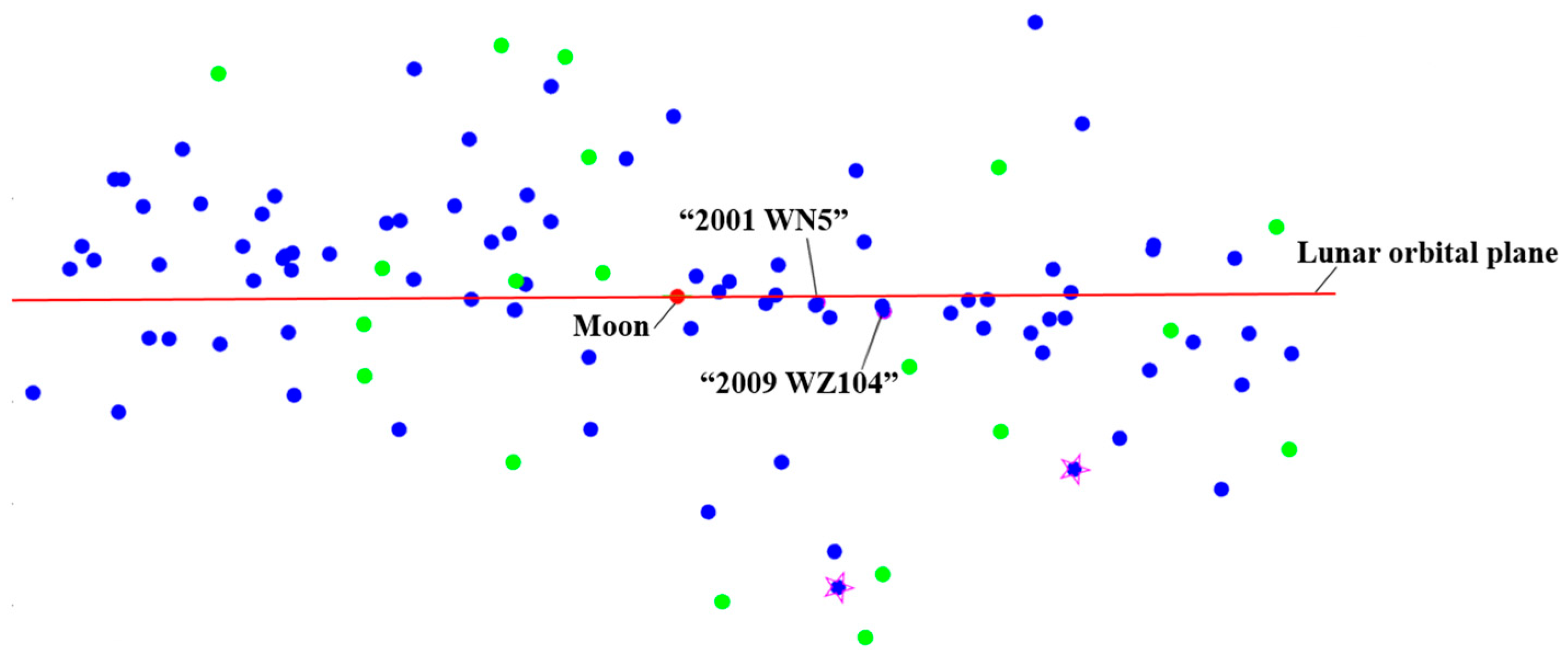
Figure 19.
The 105 flyby positions relative to the lunar orbital plane (those with one and two PHAs explored are denoted by the green and blue dots, respectively; the solutions marked by the pentagram are presented in Section 5.2).
Regarding the competition, the trajectory solutions submitted by the top five teams are presented in Table 3, where the NSSC-BACC team ranked first and reported a solution that explores 45 PHAs. The round-trip trajectories with the lowest velocity increments presented by the first- and second-place teams are shown in Figure 20 and Figure 21, respectively. The probe uses a PLF and a perigee maneuver to escape from and return to the DSS in Figure 20. However, the probe directly escapes from and returns to the DSS in Figure 21.
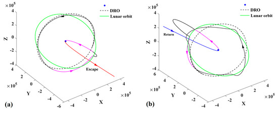
Figure 20.
The round-trip trajectory with the lowest velocity increment presented by the champion team ((a) escape flight trajectory and (b) return flight trajectory, the color change represents an orbital maneuver) (ΔV = 1.13 km/s).
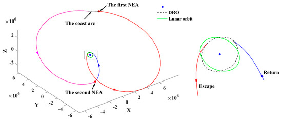
Figure 21.
The round-trip trajectory with the lowest velocity increment presented by the runner-up team (the color change represents an orbital maneuver).
5.2. Representative Trajectories
In this subsection, three representative trajectories labeled by I, II, and III in Figure 18 are presented below. Their trajectory data and optimization programs are available on the netbook (https://pan.baidu.com/s/1e2Hwg59HMTpYEhC1D8CeWQ?pwd=h02i, accessed on 26 May 2024).
- (1)
- Representative trajectory I: the minimum-ΔV round trip exploring two PHAs
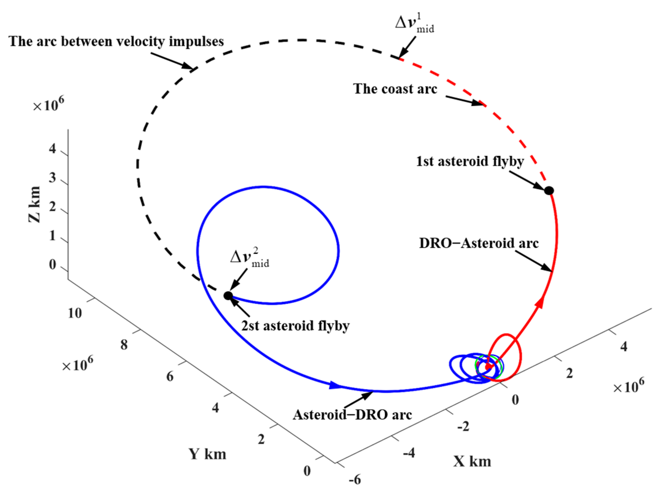
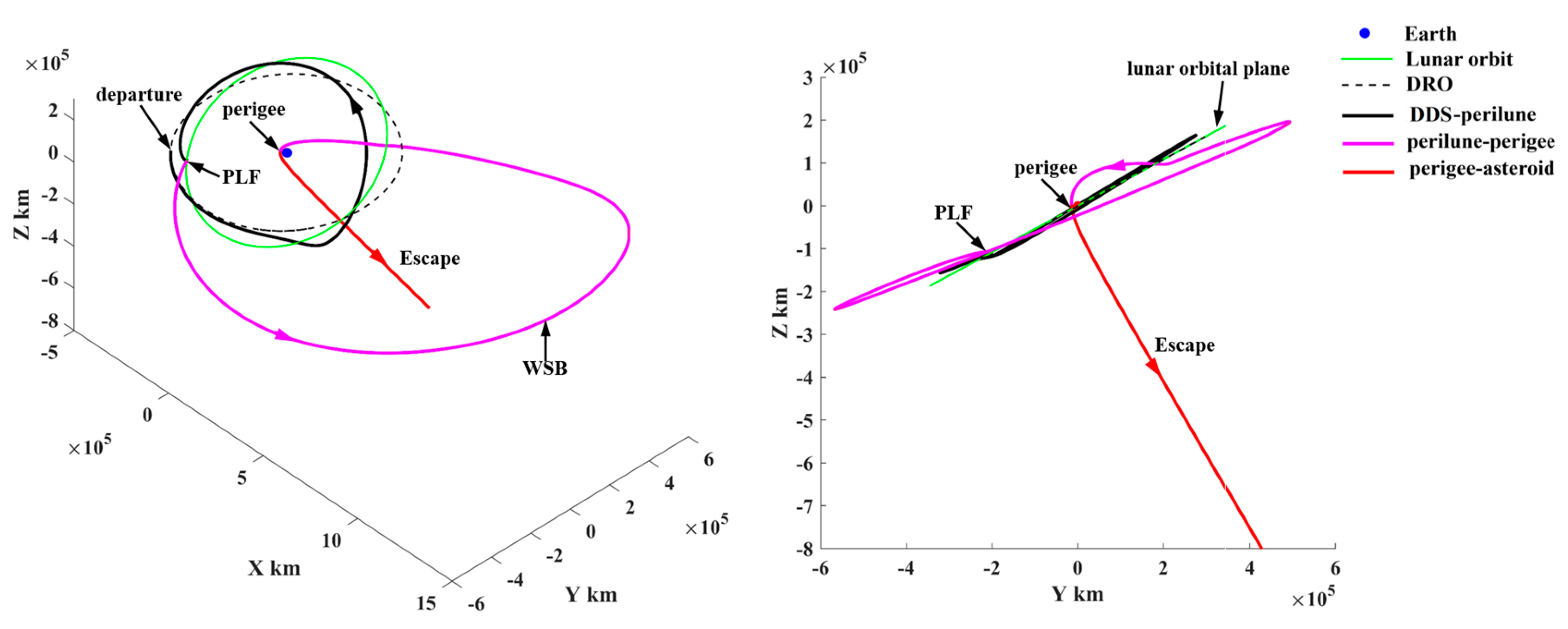
The minimum-ΔV round trip with two PHA flybys has ΔV = 635.0 m/s and TOF = 788.0 day, which is the second mission completed by probe No. 1. The round-trip trajectory is shown in Figure 22, in which the probe explores the asteroids “2001 WN5” and “2009 WZ104”. The ephemerides of these two PHAs are presented in Appendix C.
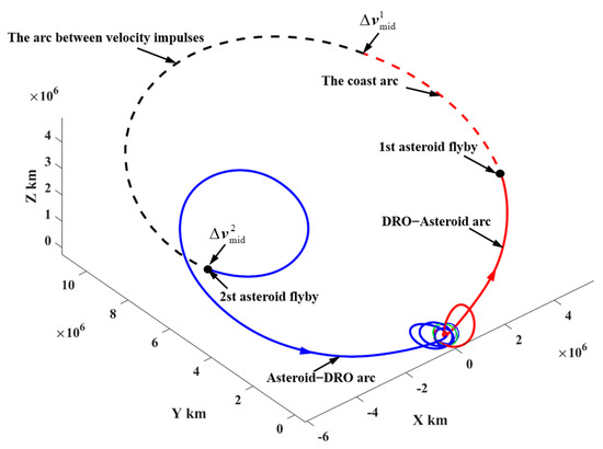
Figure 22.
The representative round-trip trajectory exploring two PHAs (in ECI).
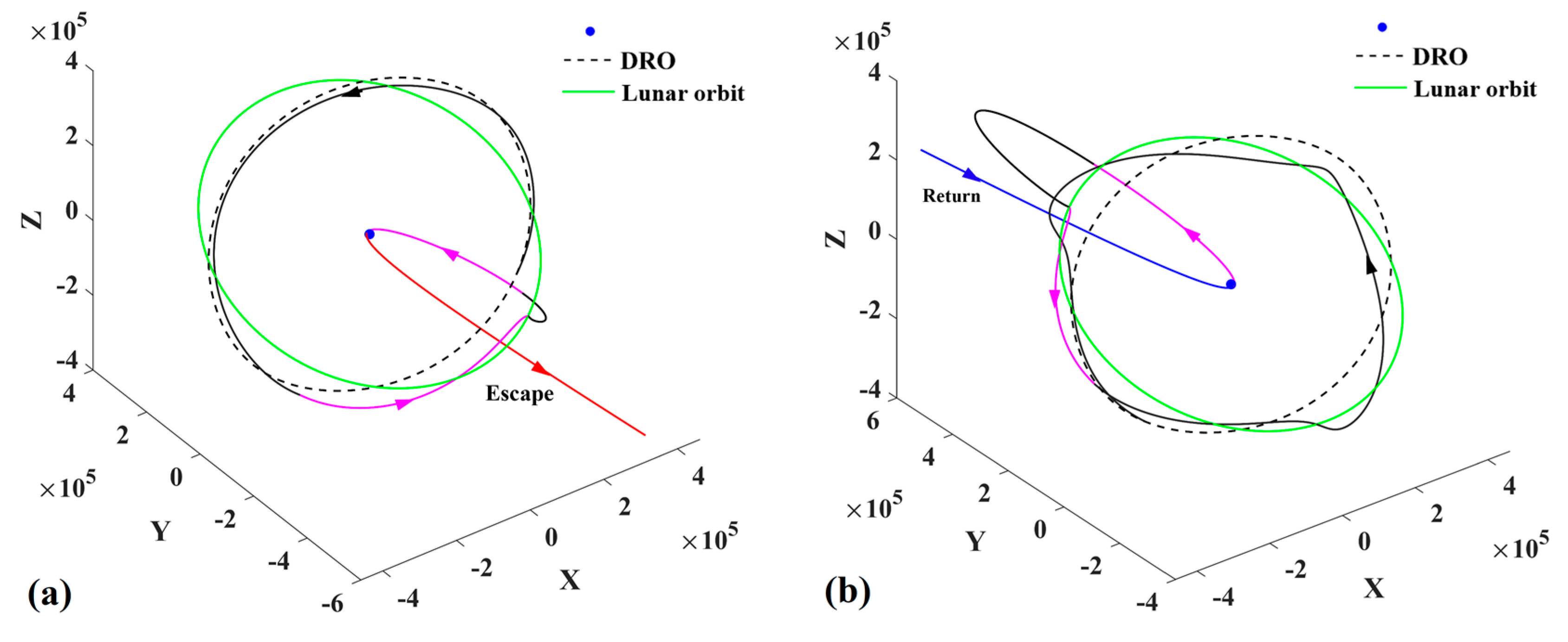
The escape/return trajectory from/to the cislunar space is shown in Figure 23. In the trajectory escape (see Figure 23a), a PLF is carried after the probe departs from the DSS, which makes the probe enter a highly elliptical orbit and reach a perigee. Then, a velocity impulse at the perigee is imposed to accelerate the orbital energy, which makes the probe escape from cislunar space finally. The return trajectory to the DSS is shown in Figure 23b. It is found that the probe first arrives at the perigee to deceleration and is captured in cislunar space. Subsequently, the probe arrives at a perilune to carry out a PLF, which makes the probe arrive at the DRO and rendezvous with the service station. Both trajectory segments use a PLF to make use of lunar gravitation. In addition, both the perilune−apogee−perigee and perigee−apogee−perilune arcs (the magenta lines in Figure 23) use the WSB ballistic transfer to change the orbital energy and the perigee height, where the apogee is far beyond the lunar orbit.
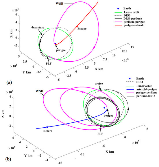
Figure 23.
(a) The trajectory segment to escape from cislunar space and (b) the return trajectory segment ending up with rendezvous of the DSS.
- (2)
- Representative trajectory II: the round trip exploring the PHA with a large inclination relative to the lunar orbital plane
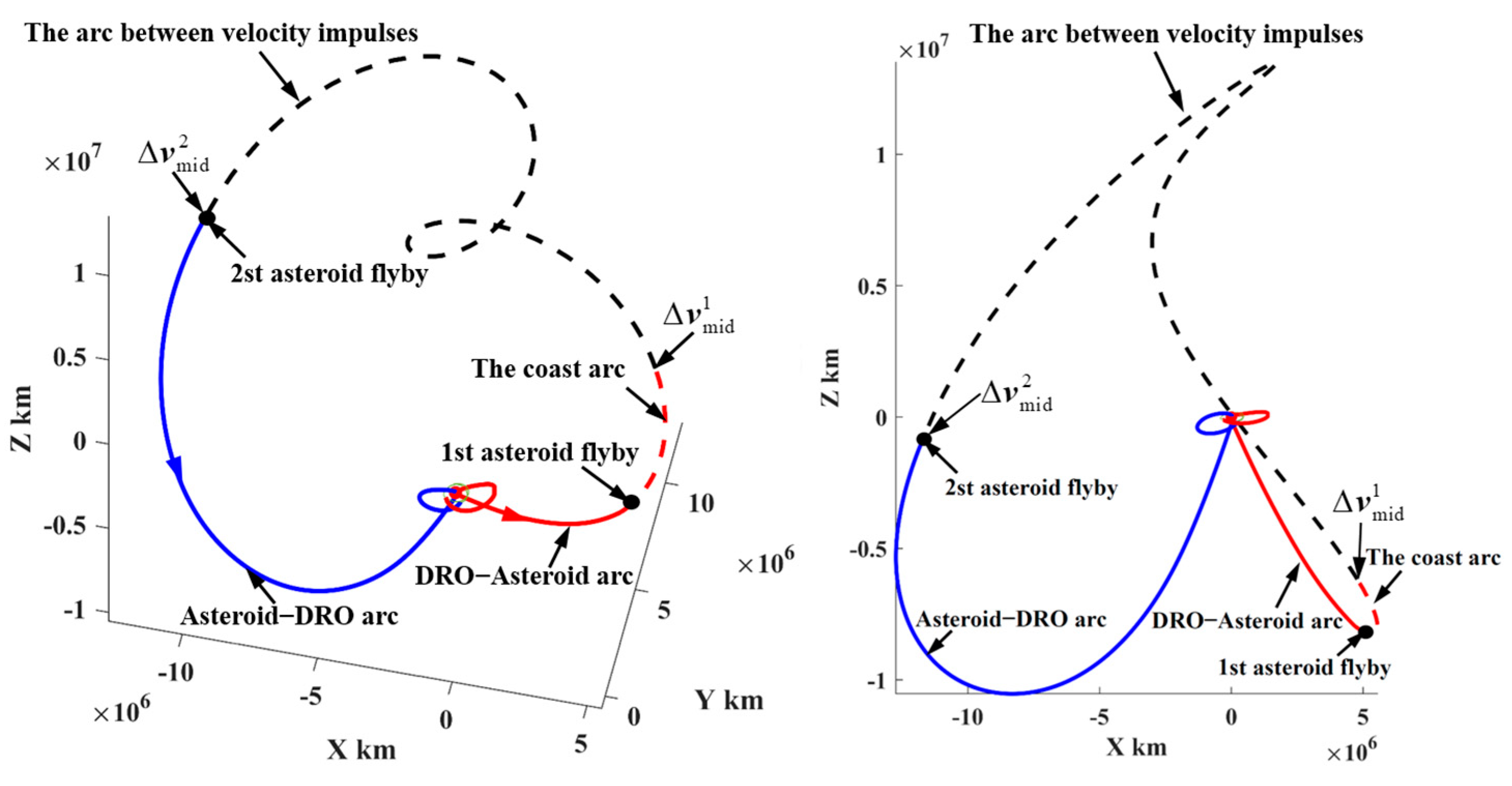
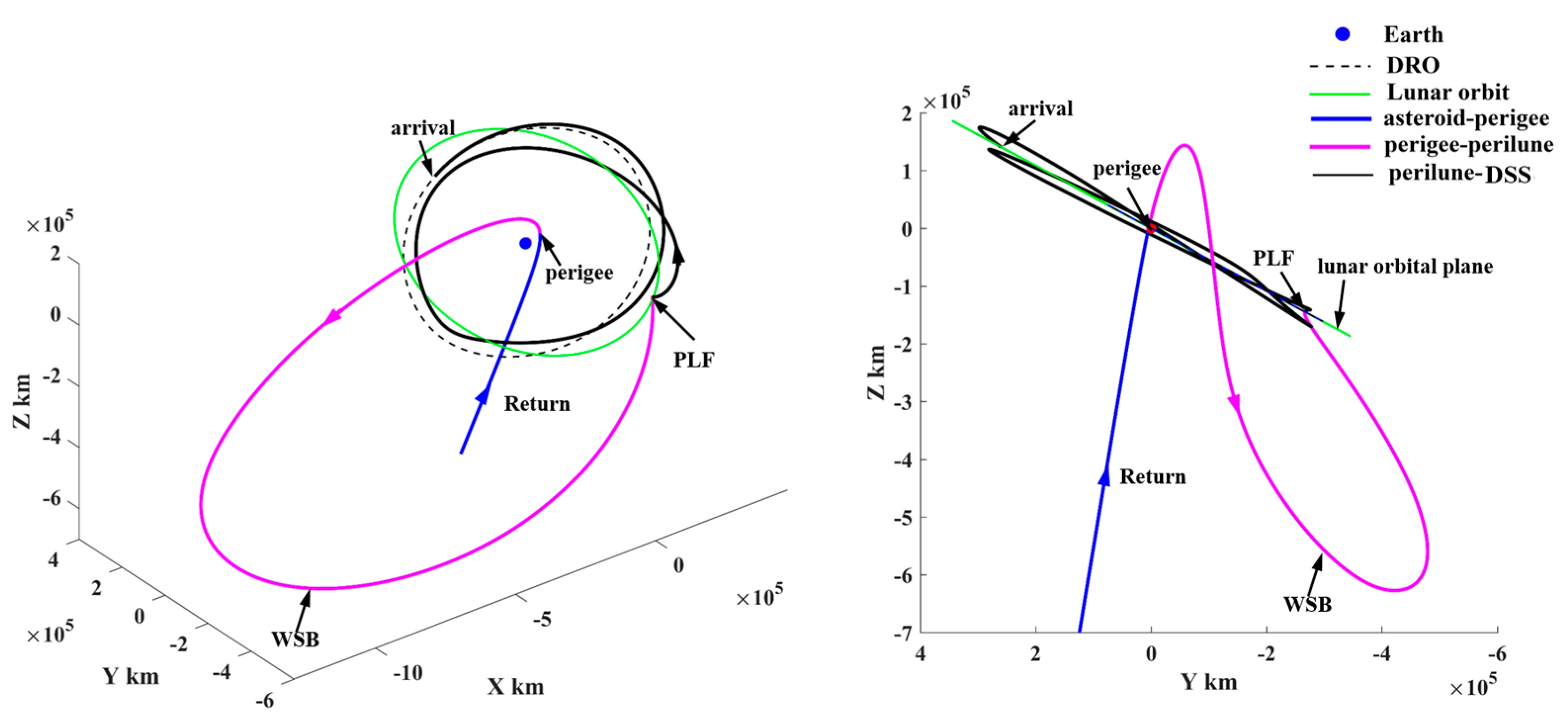
In trajectory I, the positions of the explored asteroids “2001 WN5” and “2009 WZ104” are close to the lunar orbital plane, which has a small inclination relative to the lunar orbital plane. However, the PHAs with large inclinations have also been explored. The representative trajectory II to explore two PHAs marked by the pentagram in Figure 19 is selected to display the corresponding orbital features, as shown in Figure 24, Figure 25 and Figure 26.
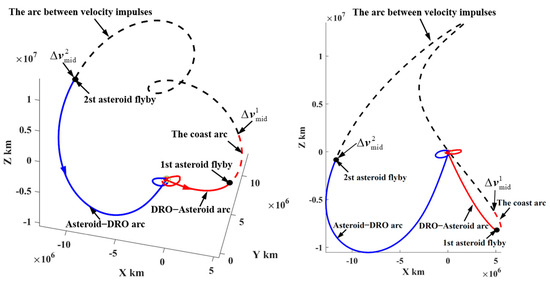
Figure 24.
A representative mission to detect two PHAs with high inclination (representative trajectory II).

Figure 25.
The trajectory segment to escape from cislunar space.
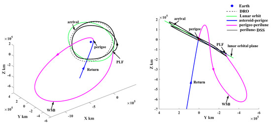
Figure 26.
The return trajectory segment ending up with rendezvous of the DSS.
In Figure 24, the depart/return trajectory from/to the cislunar space presents a large angle to the lunar orbital plane. However, the probe uses the PLF and WSB ballistic arc to change the inclination relative to the lunar orbital plane, as shown by the magenta trajectories in Figure 25 and Figure 26. Therefore, in order to explore more PHAs, especially the PHAs with large inclinations, the PLF and WSB should be introduced to the orbital design because these two strategies can launch the probe into deep space in more directions.
- (3)
- Representative trajectory III: the round trip with a single PLF to escape from (or return to) cislunar space
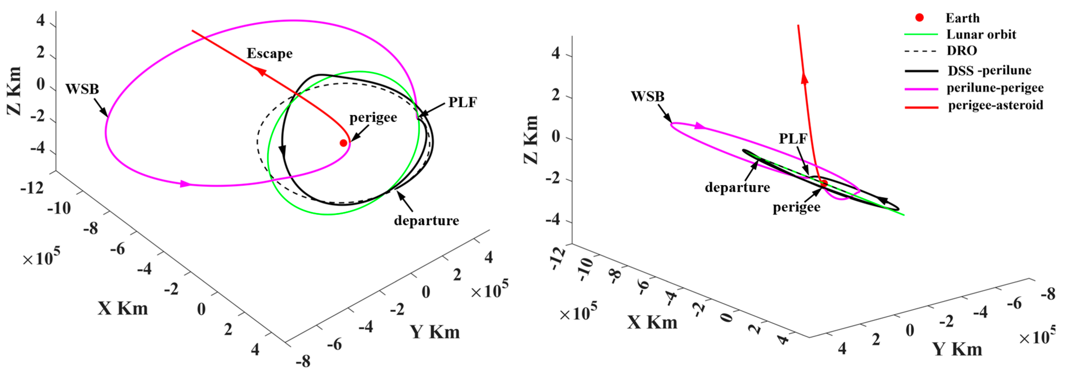
In missions I and II, the probe uses both PLF and WSB ballistic arcs to change the inclination relative to the lunar orbital plane. However, the probe can only use the PLF to change the inclination. Mission III in Figure 27 is selected to indicate the orbital features, of which both trajectory segments are shown in Figure 28 and Figure 29. It is found that the return trajectory segment only uses the PLF to change the inclination, which implies that PHA detection can also be achieved from DRO by only using PLFs.
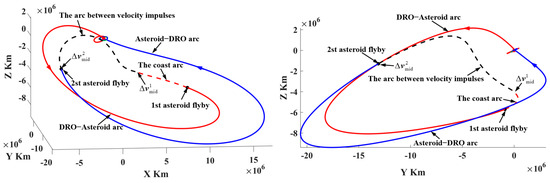
Figure 27.
The round trip with a single PLF to escape from (or return to) cislunar space (representative trajectory III).
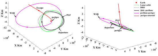
Figure 28.
The trajectory segment to escape from cislunar space.
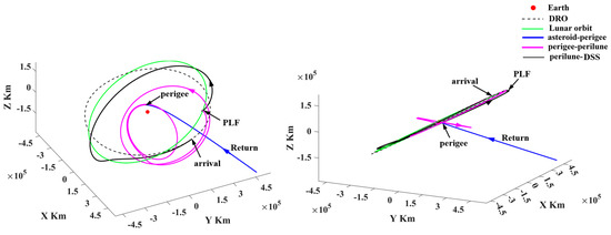
Figure 29.
The return trajectory segment ending up with rendezvous of the DSS.
6. Conclusions
The concepts of multi-probe, multi-asteroid, and multi-mission were introduced by the 12th edition of China’s Trajectory Optimization Competition (CTOC-12), which resulted in a challenging trajectory design problem that was released on 20 August 2022. The trajectory solution presented in this study shows that a total of 20 probes are capable of exploring 105 PHAs within a 10-year time interval. These design results, although not deemed globally optimal, indicate that exploring large numbers of PHAs using reusable probes is a promising option. Meanwhile, there are two highlights concerning trajectory analysis and design. First, it is found that the PLF, WSB, and perigee maneuvers play crucial roles in obtaining round-trip trajectories with a wide range of DV-TOFs. Second, taking advantage of CPU/GPU parallel computation is an effective means to achieve the trajectory solution with improved overall performance and reasonable computational time.
Author Contributions
Conceptualization, C.P. and Y.G.; methodology, C.P.; software, C.P.; validation, C.P. and Y.G.; formal analysis, C.P.; investigation, R.Z. and Y.G.; writing—original draft preparation, C.P.; writing—review and editing, C.P. and Y.G.; visualization, C.P.; supervision, Y.G.; funding acquisition, R.Z. All authors have read and agreed to the published version of the manuscript.
Funding
This research was funded by Autonomous Guidance and Control in Cislunar Space, grant number XDA30010400. the Key Laboratory Fund Project for Simulation of Complex Electronic Systems (614201004022210) and the Chinese Academy of Sciences Youth Innovation Promotion Association (2022126).
Data Availability Statement
The trajectory data are available on the netbook (https://pan.baidu.com/s/1e2Hwg59HMTpYEhC1D8CeWQ?pwd=h02i).
Conflicts of Interest
The authors declare no conflict of interest.
Appendix A. Ephemerides of the Sun and the Moon
It is assumed that the Moon and the Sun follow Keplerian orbits around the Earth, which are computed from the ephemerides given in Table A1. It is noted that the gravitational constant is for transforming the Keplerian orbital elements to the position and velocity vectors of the Sun relative to the Earth.
Table A1.
Ephemerides of Sun and Moon (referenced in ECI).
Table A1.
Ephemerides of Sun and Moon (referenced in ECI).
| Body | Sun | Moon |
|---|---|---|
| Epoch (MJD) | 60|676 | 60|676 |
| Semi-major axis/km | 149|735|127.038|2 | 391|655.927|755|148 |
| Eccentricity | 0.017|566|762|041 | 0.0 |
| Inclination/(°) | 23.436|367|962|048 | 28.443|269|963|777|8 |
| Right ascension of ascending node/(°) | 359.998|706|334|837 | 0.097|374|581|344|85 |
| Argument of perigee/(°) | 283.150|652|210|347 | 0.0 |
| Mean anomaly/(°) | 357.320|625|735|227 | 293.398|038|326|058 |
In ROT, the Moon is stationarily located in [1,0,0], and the Sun’s position and velocity vectors are calculated as follows:
where are the position and velocity vectors of the Sun expressed in ECI, is the orbital angular velocity of the Moon, and is the transformation matrix from ECI to ROT, which are given as
where , , , and are the semi-major axis, orbital inclination, right ascension, and latitude argument (the sum of argument of perigee and true anomaly) of the Moon, respectively.
Appendix B. Ephemeris of the DSS
First, the following fitting functions are used to calculate and , which are the position and velocity vectors of the DSS in ROT:
The values of each parameter of the fitting function are shown in Table A2, and is dimensionless time as follows:
where is the initial time (MJD 60676, 1 January 2025). Then, the position and velocity vectors of the DSS expressed in ECI, denoted by and , are calculated as follows:
where and are given in Equations (A2) and (A6).
Table A2.
The values of each parameter of the fitting function.
Table A2.
The values of each parameter of the fitting function.
| 1.004416792940519 | |||||
| 0.318310613651114 | 0.636620862942161 | 0.954929789574872 | |||
| −0.181970920960444 | 0.002999214058291 | −0.001841735804046 | |||
| −0.000339694958002 | 0.000008393690079 | −0.000000619177065 | |||
| 0.318309134645416 | 0.636617759107742 | 0.954929213968546 | |||
| 0.000472036321598 | 0.000015290593321 | 0.000003018234912 | |||
| 0.244768639552355 | 0.002960758097617 | 0.002650026675994 | |||
| 0.318309196516475 | 0.636621150278213 | 0.954929177067250 | |||
| 0.000644080485616 | 0.000042417828521 | 0.000013643834980 | |||
| 0.363941953749817 | −0.011999166419257 | 0.011049154388712 | |||
| 0.318310565837136 | 0.636620009522340 | 0.954930966495610 | |||
| 0.489537961370538 | 0.011846929325199 | 0.015903320386205 | |||
| 0.000853780144252 | 0.000007209074015 | 0.000053373319044 |
Appendix C. Ephemerides of the Asteroids “2001 WN5” and “2009 WZ104”
The epoch and the orbital elements for the asteroids “2001 WN5” and “2009 WZ104” are given in Table A3.
Table A3.
Ephemerides of the asteroids “2001 WN5” and “2009 WZ104” (referenced in HCI frame).
Table A3.
Ephemerides of the asteroids “2001 WN5” and “2009 WZ104” (referenced in HCI frame).
| Asteroid Name | “2001 WN5” | “2009 WZ104” |
|---|---|---|
| Epoch (modified Julian day MJD) | 59,600 | 59,600 |
| Semi-major axis/km | 1.712 | 0.8554 |
| Eccentricity | 0.4672 | 0.1927 |
| Inclination/(°) | 1.92 | 9.83 |
| Right ascension of ascending node/(°) | 277.42 | 263.260 |
| Argument of perigee/(°) | 44.60 | 10.550 |
| Mean anomaly/(°) | 30.39 | 265.48 |
The asteroids follow heliocentric Keplerian orbits that are framed in heliocentric inertial coordinates (HCI), and their orbital states in ECI are given as follows:
where and represent the position and velocity vectors of the asteroid in ECI, respectively; and represent the position and velocity vectors of the asteroid in HCI, respectively; and represent the position and velocity vectors of the Earth in HCI, respectively; and describes the coordinate transformation matrix from ECI to HCI, which is given by
where () is the angle between the ecliptic and the equatorial plane.
References
- Zhang, Y.; Michel, P. Shapes, structures, and evolution of small bodies. Astrodyn 2021, 5, 293–329. [Google Scholar] [CrossRef]
- Kawaguchi, J. The Hayabusa mission–its seven years flight. In Proceedings of the 2011 Symposium on VLSI Circuits-Digest of Technical Papers, Kyoto, Japan, 15–17 June 2011. [Google Scholar]
- Watanabe, S.-I.; Tsuda, Y.; Yoshikawa, M.; Tanaka, S.; Saiki, T.; Nakazawa, S. Hayabusa2 mission overview. Space Sci. Rev. 2017, 208, 3–16. [Google Scholar] [CrossRef]
- Lauretta, D.S.; Balram-Knutson, S.S.; Beshore, E.; Boynton, W.V.; D’aubigny, C.D.; DellaGiustina, D.N.; Enos, H.L.; Golish, D.R.; Hergenrother, C.W.; Howell, E.S.; et al. OSIRIS-REx: Sample return from asteroid (101955) Bennu. Space Sci. Rev. 2017, 212, 925–984. [Google Scholar] [CrossRef]
- Li, X.; Scheeres, D.J.; Qiao, D.; Liu, Z. Geophysical and orbital environments of asteroid 469219 2016 HO3. Astrodyn 2023, 7, 31–50. [Google Scholar] [CrossRef]
- Elvis, M. Let’s mine asteroids for science and profit. Nature 2012, 485, 549. [Google Scholar] [CrossRef] [PubMed]
- Gates, M.; Mazanek, D.; Muirhead, B.; Stich, S.; Naasz, B.; Chodas, P.; McDonald, M.; Reuter, J. NASA’s asteroid redirect mission concept development summary. In Proceedings of the 2015 IEEE Aerospace Conference, Big Sky, MT, USA, 7–14 March 2015. [Google Scholar]
- Brophy, J.; Culick, F.; Friedman, L.; Allen, C.; Baughman, D.; Bellerose, J. Asteroid Retrieval Feasibility Sstudy; Keck Institute for Space Studies, California Institute of Technology, Jet Propulsion Laboratory: Pasadena, CA, USA, 2012. [Google Scholar]
- García Yárnoz, D.; Sanchez, J.P.; McInnes, C.R. Easily retrievable objects among the NEA population. Celest. Mech. Dyn. Astron. 2013, 116, 367–388. [Google Scholar] [CrossRef]
- Lladó, N.; Ren, Y.; Masdemont, J.J.; Gómez, G. Capturing small asteroids into a Sun-Earth Lagrangian point. Acta Astronaut. 2014, 95, 176–188. [Google Scholar] [CrossRef]
- Baoyin, H.; Chen, Y.; Li, J. Capturing near Earth objects. Res. Astron. Astrophys. 2010, 10, 587–598. [Google Scholar] [CrossRef]
- Hasnain, Z.; Lamb, C.A.; Ross, S. Capturing near-Earth asteroids around Earth. Acta Astronaut. 2012, 81, 523–531. [Google Scholar] [CrossRef]
- Urrutxua, H.; Scheeres, D.; Bombardelli, C.; Gonzalo, J.L.; Peláez, J. What does it take to capture an asteroid? A case study on capturing asteroid 2006 RH120. In Proceedings of the 24th AAS/AIAA Space Flight Mechanics Meeting, San Diego, CA, USA, 26–30 January 2014. [Google Scholar]
- Stickle, A.; Rainey, E.; Syal, M.B.; Owen, J.; Miller, P.; Barnouin, O.; Ernst, C. Modeling impact outcomes for the Double Asteroid Redirection Test (DART) mission. Procedia Eng. 2017, 204, 116–123. [Google Scholar] [CrossRef]
- Mengali, G.; Quarta, A.A. Rapid Solar Sail Rendezvous Missions to Asteroid 99942 Apophis. J. Spacecr. Rocket. 2009, 46, 134–140. [Google Scholar] [CrossRef]
- Quarta, A.; Mengali, G. Electric sail missions to potentially hazardous asteroids. Acta Astronaut. 2010, 66, 1506–1519. [Google Scholar] [CrossRef]
- Li, Q.; Tao, Y.; Jiang, F. Orbital Stability and Invariant Manifolds on Distant Retrograde Orbits around Ganymede and Nearby Higher-Period Orbits. Aerospace 2022, 9, 454. [Google Scholar] [CrossRef]
- Yin, Y.; Wang, M.; Shi, Y.; Zhang, H. Midcourse correction of Earth-Moon distant retrograde orbit transfer trajectories based on high-order state transition tensors. Astrodyn 2023, 7, 335–349. [Google Scholar] [CrossRef]
- Muralidharan, V.; Howell, K.C. Stretching directions in cislunar space: Applications for departures and transfer design. Astrodyn 2023, 7, 153–178. [Google Scholar] [CrossRef]
- Lopez, F.; Mauro, A.; Mauro, S.; Monteleone, G.; Sfasciamuro, D.E.; Villa, A. A Lunar-Orbiting Satellite Constellation for Wireless Energy Supply. Aerospace 2023, 10, 919. [Google Scholar] [CrossRef]
- Strange, N.; Landau, D.; McElrath, T.; Lantoine, G.; Lam, T. Overview of mission design for NASA asteroid redirect robotic mission concept. In Proceedings of the 33rd International Electric Propulsion Conference, Washington, DC, USA, 6–10 October 2013. [Google Scholar]
- Craig, D.; Herrmann, N.; Troutman, P. The evolvable Mars campaign-study status. In Proceedings of the 2015 IEEE Aerospace Conference, Big Sky, MT, USA, 7–14 March 2015. [Google Scholar]
- Whitley, R.; Martinez, R. Options for staging orbits in cislunar space. In Proceedings of the 2016 IEEE Aerospace Conference, Big Sky, MT, USA, 5–12 March 2016. [Google Scholar]
- McCarthy, B.; Howell, K. Leveraging quasi-periodic orbits for trajectory design in cislunar space. Astrodyn 2021, 5, 139–165. [Google Scholar] [CrossRef]
- Cavallari, I.; Petitdemange, R.; Lizy-Destrez, S. Transfer from a Lunar distant retrograde orbit to Mars through Lyapunov orbits. In Proceedings of the 27th International Symposium on Space Flight Dynamics, Melbourne, Australia, 24–28 February 2019. [Google Scholar]
- Zhang, G.; Pang, B.; Sun, Y.; Zhou, X.; Shang, Y.; Chen, C.; Lu, M.; Zhang, Y.; Jin, Z.; Zhang, Y.; et al. Optimal design of Mars immigration by using reusable transporters from the Earth-Moon system. Acta Astronaut. 2023, 207, 129–152. [Google Scholar] [CrossRef]
- Belbruno, E.; Miller, J. Sun-perturbed earth-to-moon transfers with ballistic capture. J. Guid. Control. Dyn. 1993, 16, 770–775. [Google Scholar] [CrossRef]
- Yamakawa, H.; Kawaguchi, J.; Ishii, N.; Matsuo, H. On Earth-Moon transfer trajectory with gravitational capture. Adv. Astronaut. Sci. 1993, 85, 397–416. [Google Scholar]
- Peng, C.; Zhang, H.; Wen, C.; Zhu, Z.; Gao, Y. Exploring More Solutions for Low-Energy Transfers to Lunar Distant Retrograde Orbits. Celest. Mech. Dyn. Astron. 2022, 134, 4. [Google Scholar] [CrossRef]


Disclaimer/Publisher’s Note: The statements, opinions and data contained in all publications are solely those of the individual author(s) and contributor(s) and not of MDPI and/or the editor(s). MDPI and/or the editor(s) disclaim responsibility for any injury to people or property resulting from any ideas, methods, instructions or products referred to in the content. |
© 2024 by the authors. Licensee MDPI, Basel, Switzerland. This article is an open access article distributed under the terms and conditions of the Creative Commons Attribution (CC BY) license (https://creativecommons.org/licenses/by/4.0/).