Article

Robust Trajectory Planning of Gliding-Guided Projectiles with Weak Maneuverability

School of Energy and Power Engineering, Nanjing University of Science and Technology, Nanjing 210094, China
*
Author to whom correspondence should be addressed.
Aerospace 2024, 11(7), 547; https://doi.org/10.3390/aerospace11070547
Submission received: 10 May 2024 / Revised: 15 June 2024 / Accepted: 24 June 2024 / Published: 3 July 2024

Abstract

:
Due to constraints in launch platforms and cost, the maneuverability of gliding-guided projectiles is limited, necessitating a rational design of their trajectory schemes. To reduce the sensitivity of trajectory schemes to uncertainties while ensuring compatibility between flight schemes and guidance control systems and fully exploiting the control capability of the projectile, a closed-loop robust trajectory planning method is proposed. Models of major uncertain factors and state deviation at the control start point are established. Based on the NIPCE method, the stochastic dynamic model is transformed into a high-dimensional deterministic model with PCE coefficients as state variables, and the uncertainty propagation law is obtained. A PID algorithm is employed to design a tracking guidance law based on position error feedback, and open-loop and closed-loop robust trajectory planning models are established accordingly. The optimal control problem is solved by transforming it into a nonlinear programming problem using the direct shooting method. Our simulation results indicate that the NIPCE method can significantly improve the computational efficiency of uncertainty propagation while ensuring accuracy; compared with parallel MCS, the computation time is reduced by 96.8%. Open-loop robust planning can effectively mitigate the sensitivity of gliding trajectories to uncertainties (the standard deviations of terminal altitude and lateral deviations are reduced by 23.6% and 35.3%, respectively, compared to deterministic planning) but cannot completely eliminate terminal dispersion. Closed-loop robust planning effectively improves control effort consumption on the basis of open-loop planning.

1. Introduction

In the modern experiment environment, with the advancement of science and technology and the innovation of experimental concepts, the capability for beyond-visual-range precision strikes has increasingly become one of the key indicators of scientific research strength. Gliding-guided projectiles, as a new type of aircraft, combine the advantages of both tactical missiles and conventional projectiles. They not only offer low cost per shot, rapid response, and flexible use but also possess extended range and high strike accuracy, making them one of the focal directions in the current development of aircraft [1].
Among the many key technologies in research on gliding-guided projectiles, trajectory planning has always been a core and hot issue. Limited by the stringent requirements of the gun-launched platform and the harsh dynamic environment during launch, gliding projectiles are small in size with limited control fins. The navigation and control devices that can be loaded, as well as the overall structural layout of the projectile, have special requirements. Moreover, the projectile usually undergoes unpowered flight during the controlled trajectory phase. Consequently, gliding projectiles possess a low lift-to-drag ratio and limited maneuverability and anti-interference capabilities, under which the rationality of the trajectory design becomes particularly crucial [2]. Addressing this issue, Shi conducted an in-depth study on the trajectory characteristics of gliding projectiles using the energy analysis method, forming a relatively complete theoretical system [3]. Building on this, Yi planned a range-extension trajectory based on the maximum lift-to-drag ratio as the performance indicator [4]. Chen addressed the matching issues of dynamic and static parameters during the flight of gliding projectiles and proposed a full-trajectory planning method aimed at minimizing control effort as the performance indicator [5]. Following this approach, Xu introduced the concept of a composite efficiency factor, taking into account both the gliding efficiency and maneuverability of the projectile, and used it as a performance indicator to conduct trajectory design works [6]. The evolution of science and technology has given rise to an increasingly diverse array of experiment mission requirements, prompting a surge in research directions related to trajectory planning. Yan proposed a three-dimensional trajectory planning method for cruise missiles’ low-altitude penetration issues based on ant colony optimization and Bezier curve optimization, addressing the problems of excessive turning points and large turn angles common in traditional methods [7]. He employed swarm intelligence algorithms such as the grey wolf optimizer, firefly algorithm, and particle swarm optimization for maximizing the maneuver characteristics of cruise missiles and compared their respective advantages and disadvantages [8]. Liu introduced a multi-stage rapid trajectory planning algorithm based on sequential convex optimization for the online planning of multi-stage trajectories [9]. Beyond planning for individual projectiles, Liu and Pinon separately researched collaborative multiple-projectile and ‘autonomous actors-artillery collaboration’ trajectory planning [10,11]. With the advancement of science and technology, cutting-edge technologies like neural networks [12] and artificial intelligence [13] are being progressively incorporated into trajectory planning processes, demonstrating strong developmental momentum.
The aforementioned studies extensively explore trajectory planning problems from various perspectives, focusing primarily on deterministic optimal control issues; however, they do not take into account the impact of uncertainties, leading to overly idealized trajectory designs. During the actual flight of a projectile, uncertainties exist in the dynamics model, aerodynamic and environmental parameters, and states at the control start point. Planning variables, performance indicators, and constraints are closely related to these parameters, and results obtained from deterministic models may lead to exceeding variable boundaries, deviations in performance indicators, and breaches in constraint conditions. This issue can be mitigated through robust planning, which fundamentally aims to minimize the impact of uncertainties on the trajectory without eliminating or reducing the sources of uncertainty [14]. In the process of robust planning, it is critical to understand the propagation of stochastic disturbances along the trajectory under current control commands, necessitating research into quantitative methods for dynamic system uncertainties. The Linear Analysis of Covariance (LAC) method, which requires only a single integration of the error propagation equation to obtain statistical results akin to those from Monte Carlo Simulation (MCS), has been widely applied due to its efficiency in robust planning issues [15,16]. However, LAC necessitates linearized models, which can lead to significant approximation errors when dealing with highly nonlinear problems. Additionally, robust planning based on LAC is sensitive to initial conditions since it reshapes around a reference trajectory, often resulting in local optima that prematurely terminate the algorithm [17]. Given the limitations of LAC, scholars studying robust planning problems for Unmanned Aerial Vehicles (UAVs) have adopted methods based on nonlinear models such as Polynomial Chaos Expansion (PCE) [18,19,20,21,22] and Unscented Transform [23,24,25,26,27], enhancing the precision and efficiency of problem-solving.
The aforementioned studies pertain to open-loop robust planning methods, overlooking the coupling between the planned trajectory and the guidance control system. In actual conditions, deviations caused by various uncertainties are typically mitigated by the guidance control system. Consequently, the compatibility between the planned trajectory and the guidance control system significantly impacts the effectiveness of mission execution. For UAVs with ample maneuvering capability, the performance loss associated with open-loop planning does not pose a substantial issue. However, for a gliding projectile with limited rudder control capability and unpowered flight, it is critical to minimize losses and fully exploit maneuverability. Therefore, it is necessary to pursue research on robust trajectory planning methods that incorporate closed-loop feedback from the guidance control system. Nonetheless, as of now, research addressing this specific problem remains insufficient.
In summary, this paper takes a certain type of gliding-guided projectile as a case study to tackle the trajectory planning issue for striking a fixed target. To reduce the trajectory’s sensitivity to uncertainties and enhance the compatibility between the planned trajectory and the guidance control system, thereby maximizing its limited control capabilities, a closed-loop robust trajectory planning method based on the concepts of robust optimization and tracking guidance is proposed. Initially, the main uncertainties during the actual flight process of the gliding projectile are modeled, and the non-invasive polynomial chaos expansion (NIPCE) method is used to obtain quantified propagation laws for these uncertainties. Subsequently, based on these propagation results and aiming to minimize the terminal dispersion as the performance indicator, open-loop robust trajectory planning is carried out, considering the ballistic characteristics of the gliding projectile and related constraints. Furthermore, a simple yet effective Proportional-Integral-Differential (PID) controller is employed to track the robust optimal trajectory. Based on feedback from the guidance control system, the planning approach is extended to a closed-loop format, designing a closed-loop robust optimal trajectory that integrates both uncertainty factors and the ‘scheme-guidance compatibility’. Finally, through numerical simulations in various scenarios and different conditions, the impact of uncertainty deviations on the performance of closed-loop guidance is explored.

2. Models and Methods

2.1. Dynamic Model of a Gliding Ballistic

To mitigate the adverse effects of factors such as aerodynamic asymmetry and engine thrust misalignment, while reducing the cost of the guidance control system, the tail fins of gliding-guided projectiles are typically designed with a certain angle of inclination, allowing the projectile to spin slowly during flight. Consequently, only pitch and yaw control are required. In the initial design process, to facilitate the determination of the gliding projectile’s flight trajectory and main flight characteristics, its rotational motion around the center of mass is often neglected, treating it as a maneuverable point mass for study [28]. This paper is based on the following simplified assumptions.
Assumption 1. 
The gliding projectile rotates without inertia.
Assumption 2. 
The control system of the gliding projectile works ideally, without errors or delays.
The aforementioned assumptions posit that when the control mechanisms of the gliding projectile deflect, the torque acting on the projectile is in equilibrium at each instant; hence, it is termed the ‘instantaneous equilibrium’ assumption. Given its axisymmetric shape, when the total angle of attack is not excessively large, the gliding projectile exhibits linear aerodynamic characteristics.
δ z α E = m z α m z δ z δ y β E = m y β m y δ y
In the equations, δ z and δ y represent the deflection angles of the pitch and yaw control surfaces, respectively. α and β denote the angle of attack and sideslip of the projectile, with subscript E indicating the equilibrium state. m z α and m y β represent the pitch and yaw static stability derivatives, while m z δ z and m y δ y denote the control effectiveness of the pitch and yaw control surfaces, respectively.
Under the instantaneous equilibrium assumption, the control variables for the gliding trajectory can be approximated using the angle of attack α and sideslip β at equilibrium. Gliding-guided projectiles undergo unpowered flight during the controlled phase, relying on the aerodynamic forces acting on the projectile to achieve maneuver of the center of mass.
F x = q S C x 0 1 + k c α 2 + β 2 F y = q S C y α α F z = q S C z β β
In the equations, F x , F y , and F z represent the total drag, lift, and lateral force acting on the projectile, respectively. q = ρ V 2 / 2 denotes the dynamic pressure, ρ is the air density, V is the velocity of the projectile, S is the reference area of the projectile, C x 0 is the zero-lift drag coefficient, k c is the induced drag coefficient, and C y α and C z β are the partial derivatives of the lift and lateral force coefficients with respect to angle of attack and sideslip, respectively. For axisymmetric shapes, C z β = - C y α .
The centroid motion model of the gliding trajectory is
m V ˙ = m g sin θ + F x m V θ ˙ = - m g cos θ + F y m V cos θ ψ ˙ = F z x ˙ = V cos θ cos ψ y ˙ = V sin θ z ˙ = V cos θ sin ψ
In the equations, m is the mass of the projectile, g is the gravitational acceleration, θ and ψ are the inclination and deflection angle, respectively. x , y , and z are the range, altitude, and lateral displacement of the projectile, respectively.
Considering that the impact time of the gliding trajectory is free, and the target position to be hit is fixed, the range of the projectile monotonously increases and is bounded in the course of flight. In order to facilitate the follow-up analysis, the independent variable of the model was converted from time t to range x; thus, the motion model shown in Equation (3) is converted to
V ˙ = m g sin θ + F x m V cos θ cos ψ θ ˙ = m g cos θ + F y m V 2 cos θ cos ψ ψ ˙ = F z m V 2 cos 2 θ cos ψ t ˙ = 1 V cos θ cos ψ y ˙ = tan θ cos ψ z ˙ = tan ψ
Remarking the combination of state variables as X = [ V , θ , ψ , t , y , z ] T and the combination of control variables as U = [ α , β ] T , Equation (4) can be expressed as
X ˙ = f x , X , U

2.2. Model of Major Uncertainties

There exist all kinds of uncertain factors in the actual flight environment, and it is not realistic to take them all into consideration. Therefore, this paper selects the following representative uncertain factors for research, and models them as the deviation between the real value and the reference value.

2.2.1. Aerodynamic Parameter Deviation

Due to the machining errors of the projectile and variations in the ballistic environment, there are inevitably differences between the actual flight aerodynamic parameters and the reference values. This paper assumes that the deviations of the aerodynamic parameters follow mutually independent normal distributions.
C ˜ x 0 = 1 + N d σ d C x 0 C ˜ y α = 1 + N l σ l C y α C ˜ z β = 1 + N l σ l C y α
In the equations, C ˜ x 0 , C ˜ y α , and C ˜ z β represent the true values of the zero-lift drag coefficient, the lift coefficient derivative, and the lateral force coefficient derivative, respectively. Subscripts d , l and l denote the first letters of drag, lift, and lateral, respectively. N d , N l , and N l are random numbers following a standard normal distribution N(0,1), and σ d , σ l , and σ l represent the degrees to which the above parameters deviate from their reference values.

2.2.2. Meteorological Environment Deviation

The differences between actual meteorology and standard meteorology are mainly manifested in the deviations of wind field, temperature, and atmospheric density. The impact of wind field on trajectory calculation can be considered as an unmodeled random force, which is compensated by the guidance control system. Temperature primarily affects the calculation of speed of sound, thereby influencing the flight Mach number, which in turn leads to variations in aerodynamic parameters. Therefore, the deviation in temperature can be attributed to the deviation in aerodynamic parameters. In summary, this paper models the deviation in meteorological environment as the deviation in atmospheric density. The statistical characteristics of the deviation of actual atmospheric density from the standard value are related to the altitude y, and the ratio of standard deviation to standard atmospheric density can be approximated as
σ ρ = 0.003517 e y 26629.77
Therefore, the actual atmospheric density can be expressed as
ρ ˜ = 1 + N ρ σ ρ ρ
In the formula, N ρ is a random number obeying the standard normal distribution N(0,1).

2.2.3. State Deviations at the Control Start Point

Before terminal guidance begins, the full trajectory of a gliding guided projectile can be divided into four stages: the launching phase, boosting phase, climbing phase, and gliding phase, with the first three stages being uncontrolled flight [29]. After the projectile is fired, under the influence of various uncertainties, the state values at the control-start point will inevitably deviate from the designed trajectory. This paper assumes that the state deviations follow mutually independent normal distributions. Remarking X 0 = [ V 0 , θ 0 , ψ 0 , t 0 , y 0 , z 0 ] T as the design value of the trajectory at the control-start point, then the actual state at the control start point can be expressed as
X ˜ 0 = V ˜ 0 θ ˜ 0 ψ ˜ 0 t ˜ 0 y ˜ 0 z ˜ 0 = V 0 + N V σ V θ 0 + N θ σ θ ψ 0 + N ψ σ ψ t 0 + N t σ t y 0 + N y σ y z 0 + N z σ z
In the equations, N V , N θ , N ψ , N t , N y , and N z are random numbers obeying the standard normal distribution N(0,1) and σ V , σ θ , σ ψ , σ t , σ y , and σ z represent the standard deviation of each state at the control-start point, respectively.

2.3. Uncertainty Propagation of the Gliding Trajectory

2.3.1. Transformation of the Stochastic Dynamic Model

Based on the discussion in Section 2.2, the main uncertainties during the flight of a gliding projectile can be categorized into two types: parameter uncertainties and initial state uncertainties. The dimension of parameter uncertainties d P = 4 , while the dimension of initial state uncertainties d X = 6 . Therefore, the dimension of uncertainty factors for the entire stochastic dynamic system d = 10 . Remarking the random parameters as P = [ σ d , σ l , σ l , σ ρ ] T and introducing them into the dynamic system shown in Equation (4), then the stochastic dynamic model can be expressed as
X ˙ = f x , X , U , P
This paper adopts the NIPCE method based on Gaussian quadrature node sampling and the Weighted Stochastic Response Surface Method (WSRSM) [30] to transform Equation (10) into a high-dimensional deterministic dynamic model with PCE coefficients as state variables. Setting the order of PCE as p = 2 , then the number of PCE coefficients corresponding to each state variable after expansion is
P + 1 = p + d ! p ! d ! = 66
The number of sampling points used for regression is
n s = 2 P + 1 = 132
According to the theory of generalized polynomial chaos, each state variable in Formula (10) can be expanded in the form of a polynomial.
X i j = 0 P S i j Φ j ξ ,   i = 1 , 2 , , d X
In the equation, ξ R 10 is a d -dimensional cell array, where each element consists of n s Gaussian quadrature sampling points corresponding to the respective uncertain factors. Let the univariate orthogonal basis functions corresponding to each uncertain factor in each dimension be denoted by ϕ j ( ξ k ) ,   k = 1 , 2 , , d ; then, Φ j ( ξ ) represents the orthogonal polynomial function obtained by taking tensor products of ϕ j ( ξ k ) . S i j denotes the j-th PCE coefficient of the i-th state variable, and the total number of coefficients is
n PCE = d X P + 1 = 396
For the random parameters which obey the normal distribution, the first-order, one-dimensional orthogonal polynomial model can accurately describe the uncertainty [31]. Therefore, each random parameter can be expanded in the form of the sum of 2 terms.
P i = p i 0 Φ 0 ξ P + p i 1 Φ 1 ξ P ,   i = 1 , 2 , , d P
In the equation, ξ P R 4 is a d P -dimensional cell array, where each element consists of n s Gaussian quadrature sampling points corresponding to the respective uncertain factors.
To sum up, the stochastic system shown in formula (10) is transformed into
Ψ S ˙ PCE = F x , S PCE , U , P PCE
In the formula, S PCE R 396 denotes the PCE coefficients of all state variables, P PCE R 8 denotes the PCE coefficients of random parameters, F R 792 is the actual response values of n s sample points into the original stochastic system Formula (10), and Ψ R 792 × 396 denotes the coefficient matrix of the transformed deterministic system which is described in detail as follows.
Remarking Ω ( ξ i ) = [ Φ 0 ( ξ i ) , Φ 1 ( ξ i ) , Φ P ( ξ i ) ]   , i = 1 , 2 , , n s , defining the intermediate matrix as
Θ ( ξ i ) R 6 × 396 = I d X Ω ( ξ i )
In the equation, the symbol denotes the Cronecker product; therefore,
Ψ = [ Θ ( ξ 1 ) T , Θ ( ξ 2 ) T , Θ ( ξ n s ) T ] T
Considering the different importance of each sample point, the weight vector is
ω s R 792 = [ ω T , ω T , , ω T ] a   total   of   d X   items T
In the formula, ω denotes the weight corresponding to n s sample points.
So far, according to the WSRSM, the overdetermined equations shown in formula (16) can be solved by weighted least-squares regression.
H = Ψ T W s Ψ 1 Ψ T W s S ˙ PCE = H F x , S PCE , U , P PCE
where H R 396 × 792 is the regression coefficient matrix and W s R 792 × 792 = diag ( ω s ) denotes the weight matrix.
By numerical integration of Equation (20), the variation of all PCE coefficients with range x can be obtained. The mean μ and standard deviation σ of the state variables in the original stochastic system can be obtained directly from the PCE coefficients.
μ X i = S i 0 σ X i = j = 1 P S i j 2 E Φ j 2 ξ   ,   i = 1 , 2 , , d X
where the operator E represents the mathematical expectation.

2.3.2. Truncation of Chaotic Polynomial Basis

According to the description in Section 2.3.1, the transformed deterministic system has a total of 396 state variables, and there are also 132 Gaussian quadrature sampling points used for regression. In this problem scale, the computation time for a single uncertainty propagation is acceptable. However, in subsequent robust trajectory planning of the gliding projectile, the uncertainty propagation module will be repeatedly called during the iterative process. Moreover, the convergence speed of optimization algorithms significantly decreases when the number of variables is large, leading to a significant reduction in computational efficiency.
It is known that as the dimension d of the uncertainty factors increases, the total number of terms in the orthogonal polynomials grows exponentially. However, in many problems, not all terms in the polynomial expansion are equally important. Typically, only a few variables are involved in the important terms of the expansion. In most practical engineering systems, the output response is mainly influenced by the input variables and their low-order interaction terms, while the impact of higher-order interaction terms is relatively small.
Considering the above analysis, this paper adopts a maximum interaction restriction truncation strategy to directly remove high-order polynomial terms, thereby reducing the computational burden.
In the full-order PCE model (13), multivariate orthogonal polynomials are constructed by the direct tensor product. When the PCE order is p , it is necessary that
A d , p = λ N d : λ 1 j = 1 d λ j   p
In the formula, λ = [ λ 1 , λ 2 , , λ d ] represents multiple indexes, A d , p is a set of multiple indexes, λ i is the order of the base of univariate orthogonal polynomials corresponding to the j-dimensional variables in multivariate orthogonal polynomials, and the operator 1 represents 1-norm.
The main idea of maximum interaction restriction truncation is to select a low rank subset A d , p , r from the multi-index set defined in Formula (22) to ensure not only λ 1   p  but also λ 0   r .
A d , p , r = λ A d , p : λ λ 0   p 1     r < min d , p
In the equations, λ 0 represents the rank of multiple indexes and r represents the truncation coefficient.
For the case study in this paper, d = 10 and p = 2 . Therefore, based on Equation (23), the truncation coefficient is set to r = 1 . After removing the high-order interaction terms, the number of PCE coefficients for each dimension of random variables decreases from 66 at full order to 11. Consequently, the total number of state variables in the deterministic dynamic system after dimensionality reduction decreases from 396 to 66. The number of Gaussian quadrature sampling points used for regression decreases from 132 to 22, representing a reduction of 83.3%.

2.4. Robust Planning Model of Gliding Trajectories

2.4.1. Open-Loop Robust Planning

1.
Planning expectation
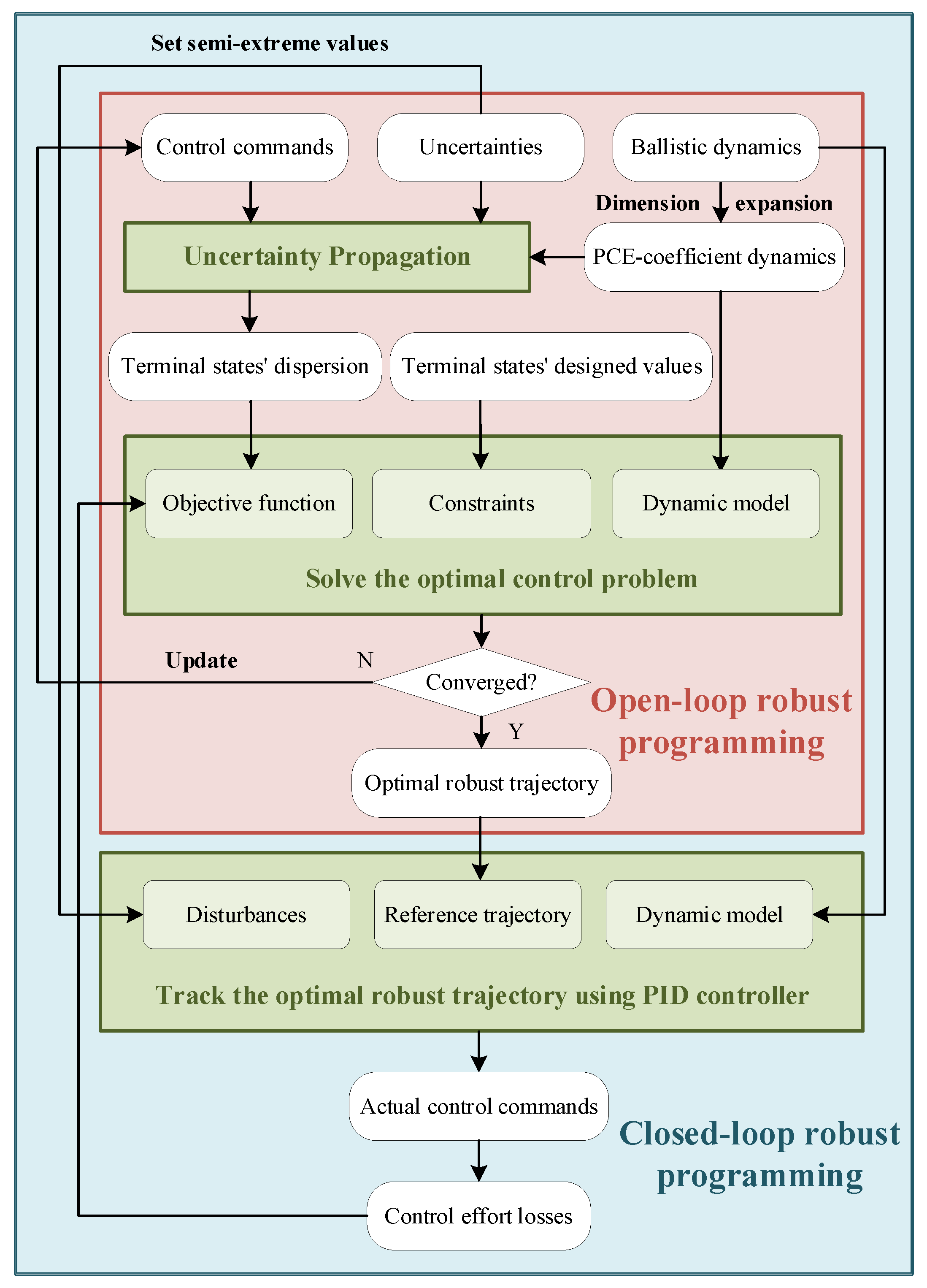
With the control variables determined, through the method introduced in Section 2.3, one can accurately and efficiently obtain the propagation laws of uncertainties along the gliding trajectory. This is manifested as deviations and dispersion of the trajectory envelope during the flight process and terminal states. By incorporating the results of uncertainty propagation into the objective function and constraints during trajectory planning, the robustness of the trajectory can be enhanced in the iterative process, reducing the sensitivity of the gliding trajectory to random disturbances.
Theoretically, statistical information about the terminal states of the trajectory can be obtained through the PCE agent model, allowing the covariance ellipse of the terminal states to be determined. Bringing back the control variables of the robust optimal trajectory to the original stochastic dynamic model for open-loop tracking enables the true distribution of the gliding trajectory’s terminal position to be obtained. By observing the coverage of the theoretical covariance ellipse on the actual terminal position, the effectiveness of robust planning can be validated, with the expected results depicted in Figure 1.
2.
Dynamics model
The dynamics model is the deterministic system shown in Equation (16) after dimensional expansion, the state variables are all PCE coefficients, and the control variables are consistent with the original stochastic system.
3.
Constraints
After considering the influence of uncertain factors, there are numerous results (bounded) of flight trajectory under the same open-loop control input. Therefore, the focus of open-loop robust planning is not the specific values of the states, but their statistical laws, and the statistical moments of state variables should also be considered in the constraints (this paper mainly focuses on the first and second order statistical moments, which are mean and variance).
  • Boundary constraints
According to the analysis in Section 2.2.3, the state deviations at the control-start point obey the independent normal distribution. Therefore, the constraints of the mean of initial states are
E V x 0 = V 0 ,   E θ x 0 = θ 0 ,   E ψ x 0 = ψ 0 E t x 0 = t 0 ,   E y x 0 = y 0 ,   E z x 0 = z 0
where x 0 = 0  is the x coordinate at the control start point.
In order to ensure the final strike accuracy and strike effect, the constraints on the mean values of the terminal states are
E V x f     V f min ,   E y x f = y T ,   E z x f = z T
In the formulas, the subscript f represents the first letter of final, the subscript T represents the first letter of Target, x f = x T , and ( x T , y T , z T ) represents the fixed target position.
  • Path constraints
Considering the limited rudder control capabilities of the gliding projectile, the control constraints during flight are
α     α max ,   β     β max
4.
Objective function
For the planned trajectory of a gliding projectile, the dispersion at the terminal position is usually used as a criterion to measure its sensitivity to uncertainty, while less attention is paid to the dispersion of other terminal states and the state envelope during the flight. Therefore, the objective function of the open-loop robust planning is designed as
min J o = D y f + D z f
In the formula, the subscript o represents the first letter of the open-loop and the operator D represents the variance.

2.4.2. Closed-Loop Robust Planning

1.
Planning Expectation
Closed-loop robust planning builds upon open-loop planning by incorporating a tracking guidance module. It assumes that all uncertainties are biased towards the semi-extreme (which means the ± 1.5 σ value of each random parameter in this paper). The tracking of robust optimal trajectories provides closed-loop feedback for control variables, thus obtaining control effort consumption during the projectile’s flight (based on simulation experiences and measured data, the condition where all uncertainties are biased to the semi-extreme is quite stringent, making trajectory tracking relatively challenging and control effort consumption higher. Adopting such a conservative approach during the planning process can generally ensure the smooth progress of closed-loop guidance during actual flight). By incorporating control effort consumption as a penalty function into the planning objective function, the iterative process can then consider the coupling and matching characteristics between the planned trajectory and the guidance system, enabling the planning of a closed-loop robust optimal trajectory that balances robustness and feasibility.
2.
Closed-loop guidance based on PID control
Due to the repeated invocation of the guidance module during the iterative process of closed-loop planning algorithms, a sufficiently simple and effective trajectory-tracking algorithm is necessary. In the existing literature, some scholars employed the Linear Quadratic Regulator (LQR) algorithm for tracking programmed trajectories [17]. This method involves linearizing the model near the reference trajectory, which can lead to significant tracking errors when deviations are large. Furthermore, the LQR algorithm requires solving the Riccati equation, increasing the complexity of the solution. Based on the aforementioned analysis, this paper utilizes a PID controller with an analytic expression that does not rely on the model for tracking the planned trajectory. Let the altitude and lateral displacement at the range x on the reference trajectory be denoted as y ^ and z ^ , respectively, and the control variables as U ^ ; then, the position error of the projectile relative to the reference trajectory can be expressed as
e = e y e z = y ^ y z ^ z
The closed-loop control commands after feedback modification can be expressed as
U c = α c β c = U ^ + Δ U = U ^ + Δ α Δ β = U ^ + k P e + k I x 0 x e   d τ + k D e ˙
In the formula, the subscript c represents the first letter of closed-loop. k P , k I , and k D represent proportional parameter, integral parameter, and differential parameter, respectively. The minus sign in front of Δ β item indicates the direction.
3.
Dynamic model and constraints
The dynamic model and related constraints of closed-loop robust planning are the same as those in open-loop planning, which need not be repeated.
4.
Objective function
Defining the closed-loop control effort consumption of the projectile during flight as
E c = x 0 x f α c 2 + β c 2   d x
Then, the objective function of closed-loop robust planning can be designed as
min J c = ω D J o + E c
where ω D is the weight of the terminal position dispersion.
Closed-loop robust trajectory planning is a multi-objective optimal control problem. Considering that the order of magnitude difference between J o and E c in the calculation example is large, in order to achieve the balance of planning emphasis, this paper uses the deterministic energy-optimal trajectory without considering random disturbance as the benchmark trajectory to make the objective function dimensionless. Remarking the terminal position dispersion of the benchmark trajectory after uncertainty propagation as J ¯ and the control effort consumption as E ¯ , then the objective function is converted into
min J c = ω D J o J ¯ + E c E ¯

2.4.3. Flow of Robust Gliding Trajectory Planning

In summary, the open-loop robust planning problem of gliding trajectory can be described as follows: considering the main uncertain factors discussed in Section 2.2 and the high-dimensional deterministic dynamic model shown in Equation (16), planning the open-loop control commands U o within a known range [ x 0 , x f ] based on the current environment and task requirements. After uncertain factors propagate along the gliding trajectory under the action of U o , the flight scheme can minimize the objective function shown in Equation (27) while satisfying the constraint Equations (24) to (26). The closed-loop robust planning problem can be described as follows: taking the open-loop robust optimal trajectory as the reference trajectory, considering the case where all uncertain factors are shifted to semi-extreme, obtaining the feedback-modified closed-loop control commands U c through the PID controller shown in Equation (29) and calculating the control effort consumption E c , incorporating E c into the planning objective in the form of penalty functions. Using the deterministic energy-optimal trajectory as the benchmark, non-dimensionalizing the objective function as shown in Equation (32), obtaining the closed-loop robust optimal trajectory through a bi-level planning format. The flow chart of gliding trajectory robust planning proposed in this paper is shown in Figure 2.

3. Simulation Results and Analysis

Due to the large number of states in the deterministic system after dimension-expansion and the presence of many zero elements in the PCE coefficients, the problem scale is large. Discretizing state variables will cause unnecessary computational time consumption. Meanwhile, the uncertainty propagation module only needs control input information to obtain the statistical laws of the system states that meet the accuracy requirements. Therefore, this paper adopts a direct shooting method with only discrete control variables to solve the robust planning problem of gliding trajectory, with the number of discrete points N set to 65. The relevant parameters of the projectile and target are shown in Table 1, and the parameters related to uncertainty are shown in Table 2. The parameters of the PID controller are adjusted and adapted during the simulation process, set to k P = 1.0 × 10 2 , k I = 1.5 × 10 10 , and k D = 1.2 × 10 1 .

3.1. Uncertainty Propagation of Gliding Trajectory under Specified Control Commands

When uncertainty factors are not considered, conducting trajectory planning based on minimizing control effort consumption as the objective function can yield the deterministic optimal control commands U ^ , which is not detailed in this paper. To verify the effectiveness and superiority of the NIPCE method proposed in this paper, according to the discussion in Section 2.3, substituting U ^ into the high-dimensional system Equation (16) for uncertainty propagation, the simulation results are shown in Figure 3 (where the symbols μ ( ) and σ ( ) represent the mean value and standard deviation of the state variables, the black dotted lines in the figures represent the constraint thresholds of the state variables, and in the legend, FOPCE and COPCE respectively denote the full-order PCE and cutoff-order PCE).
From the results in Figure 3a,i,k, it is obvious that under the influence of various uncertain factors, the mean value of state at the end of the trajectory violates the constraint conditions indicated in Equation (25). From Figure 3j,l, it can be observed that there is a significant dispersion in the terminal position of the trajectory. Therefore, robust planning of the gliding trajectory is required to modify the deviations in state and reduce the impact of uncertainty factors. Furthermore, by observing all subplots in Figure 3, it is noted that the results of the FOPCE method are highly consistent with the MCS results. When using the basis-truncation strategy (corresponding to the COPCE method) to eliminate high-order polynomial terms, the standard deviations of the terms V , θ and ψ with relatively high nonlinearity (Figure 3b,d,f) in Equation (4) show some deviation from the MCS results, but within an acceptable range of accuracy. The deviation occurs only during intermediate processes, with the statistical characteristics at the end of the trajectory remaining unaffected. This analysis illustrates that the NIPCE method proposed in this paper is competent for quantifying the uncertainties of gliding trajectories, and in subsequent robust planning processes, a truncated PCE model can be used instead of a full-order PCE model to enhance computational efficiency.

3.2. Open-Loop Robust Planning

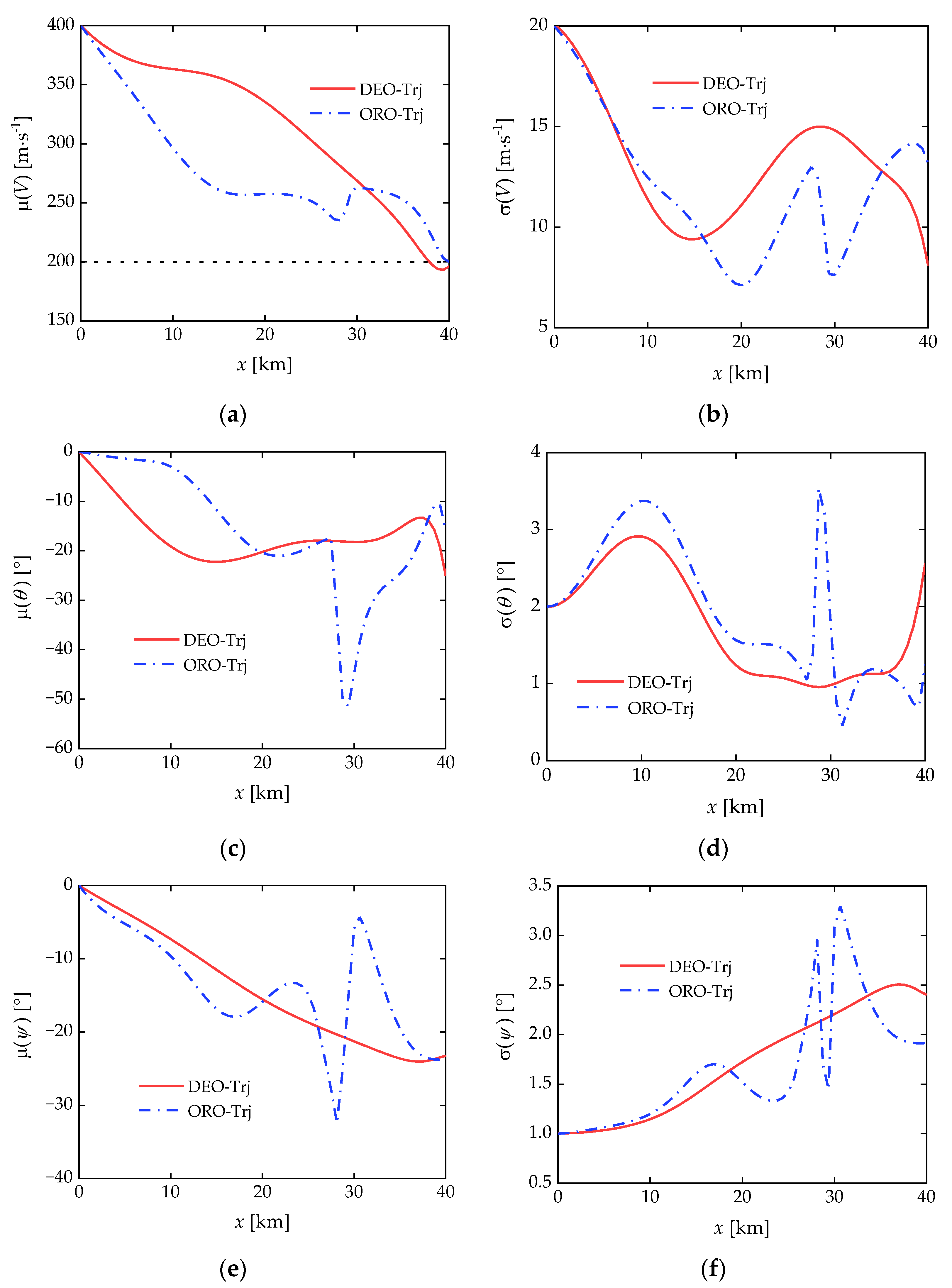
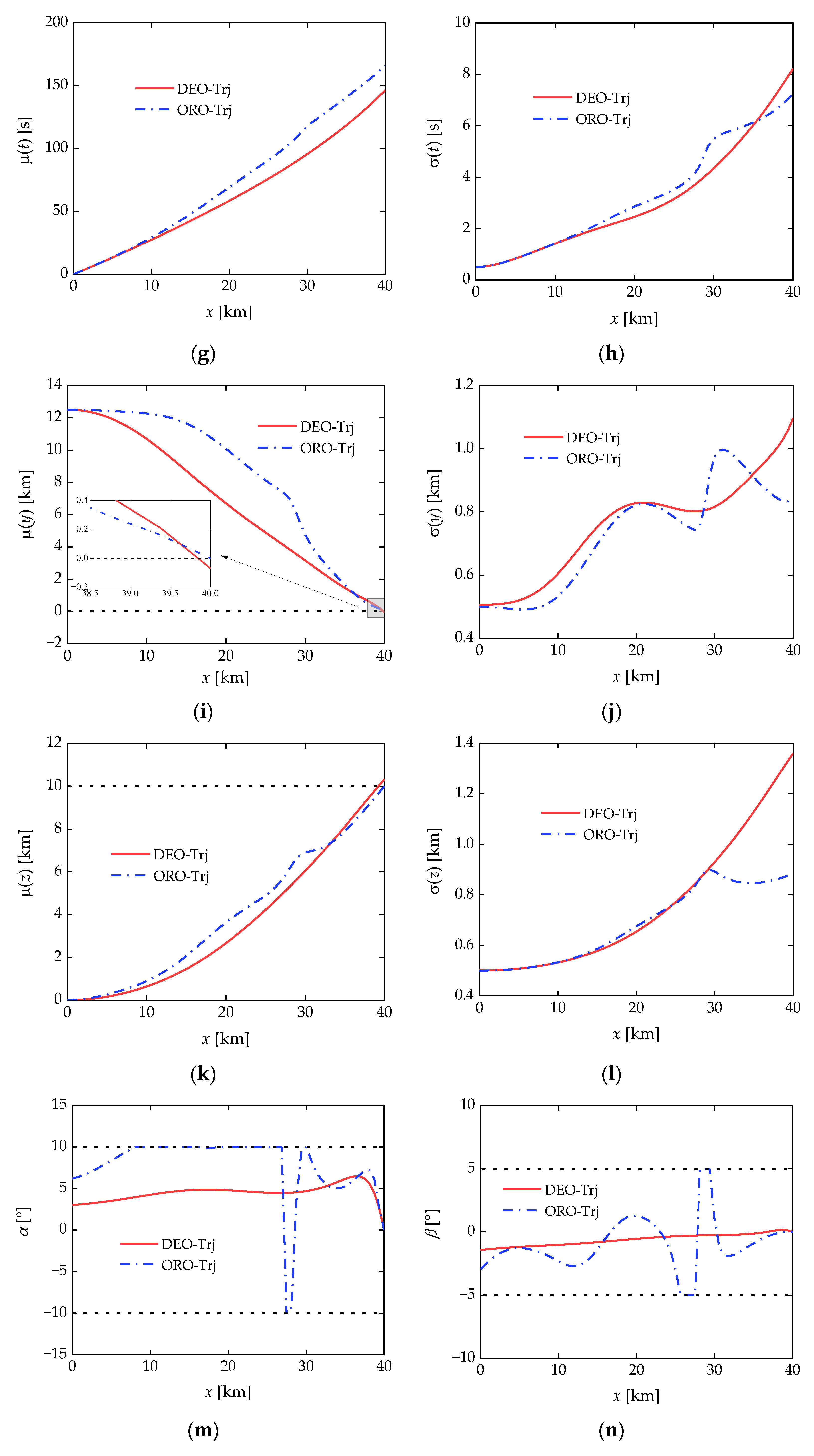
Based on the discussion in Section 2.4.1, using the deterministic effort-optimal control commands U ^ as the initial value for iteration, the open-loop robust planning results of the gliding trajectory are shown in Figure 4 (in the legend, DEO-Trj represents the results of uncertainty propagation along the trajectory under the influence of U ^ , and ORO-Trj represents the uncertainty propagation results of the open-loop robust optimal control commands U o ).
Based on Figure 4a,i,k, open-loop robust planning corrects the bias in the mean value of terminal states of the trajectory, ensuring compliance with the constraints outlined in Equation (25). Figure 4a,g,i,k show that the curvature in the middle section of the robust optimal trajectory increases compared to the reference trajectory, resulting in reduced projectile velocity and a longer flight time. This implies that increasing the mid-trajectory curvature enhances the robustness of the planned trajectory, aligning with the conclusions drawn using the LAC method in reference [2]. Figure 4j,l reveal that the open-loop robust planning significantly reduces the dispersion at the trajectory’s terminal point, with standard deviations of altitude and lateral deviation decreasing by 23.6% and 35.3%, respectively. This effectively minimizes the sensitivity of the planned trajectory to uncertainties. However, as observed in Figure 4m,n, the control commands of the robust optimal trajectory significantly increase compared to the reference trajectory, indicating that the trajectory’s robustness is achieved at the expense of additional control effort consumption. Moreover, the results demonstrate that the projectile remains at control saturation for a considerable period, posing significant challenges to subsequent guidance control system design. If the deviation of uncertainties is substantial, a gliding projectile with limited maneuverability may fail to track the planned trajectory, leading to mission failure. Therefore, considering the alignment between the planned trajectory and the guidance control system during planning, conducting closed-loop robust trajectory planning research holds significant practical importance.

3.3. Closed-Loop Robust Planning

Based on the discussion in Section 2.4.2, considering the scenario where uncertainties are skewed to the semi-extreme values, a PID controller is used to track the open-loop robust optimal trajectory, providing closed-loop feedback for control commands. The closed-loop control effort consumption is calculated and incorporated into the objective function. This paper employs the weight of terminal position dispersion ω D in Equation (32) as the basis for distinguishing the following three scenarios.
Scenario 1: ω D = 0 , which indicates that the terminal dispersion is allowed, only the state deviations are modified, and the control effort consumption is minimized.
Scenario 2: ω D = 1 , which means that both terminal dispersion and control effort consumption are taken into consideration, and both are equally important.
Scenario 3: ω D = 5 , which means taking both the terminal dispersion and the control effort consumption into consideration, but the former is more important.
Scenario 4: ω D = 100 , which indicates that the terminal dispersion term is of significant importance while the weight of the control effort consumption term can be ignored.
The results of the closed-loop robust planning of gliding trajectory in different scenarios are shown in Figure 5.
From the results in Figure 5, it is evident that with the introduction of a guidance control module, the closed-loop robust planning outcome is no longer a statistical law. The projectile, under the influence of the guidance law, precisely hits the target, eliminating terminal dispersion. Even under relatively stringent deviation conditions, the projectile still manages to track the reference trajectory with minimal control saturation (It can be imagined that with smaller deviations, the projectile’s control effort consumption would be lower). This proves the effectiveness and superiority of closed-loop planning.
As the terminal dispersion weight ω D increases, the curvature in the middle section of the closed-loop robust optimal trajectory correspondingly increases, gradually approaching the open-loop robust optimal trajectory (as shown in Figure 4i,k), and the control commands also increase accordingly. It can be inferred that when ω D is sufficiently large, the proportion of control effort consumption in the objective function Equation (32) will approach zero. The closed-loop robust planning will degenerate into open-loop robust planning, and the closed-loop robust optimal trajectory will converge to the open-loop robust optimal trajectory.

3.4. Influence of the Uncertain Factors’ Deviation Degree on Closed-Loop Guidance

In the process of closed-loop robust trajectory planning, all uncertain factors are biased to the semi-extreme situation, which is a conservative approach. According to relevant simulation experiences and measured data, the degree of deviation of each random parameter during the actual flight of the gliding projectile is not the same. Therefore, based on the degree of deviation of uncertain factors, this paper distinguishes the following four conditions.
Condition 1: The deviations of uncertain factors are all set to corresponding + 3 σ values to simulate the upper bound of the extreme deviation situation.
Condition 2: The deviations of uncertain factors are alternately set to the corresponding + σ and σ values to simulate the actual flight environment.
Condition 3: The deviations of uncertain factors are all set to corresponding 3 σ values to simulate the lower bound of the extreme deviation situation.
Condition 4: Except for the velocity deviation at the control-start point set to σ V , the deviations of other uncertain factors are still set to the corresponding 3 σ values. Condition 4 serves as an additional control group for Condition 3.
Taking Scenario 3 in Section 3.3 as an example, using the closed-loop guidance law based on the PID controller designed in this paper, the tracking effects of the gliding projectile on the planned trajectory under different conditions are shown in Figure 6 (Ref-Trj in the legend represents the reference trajectory, Act-Trj represents the actual trajectory, and the suffix C is used to distinguish conditions).
The results from Figure 6 indicate that under different conditions, the projectile has successfully tracked the planned trajectory in the lateral plane, while the tracking situation in the longitudinal plane is relatively complex. Specifically, the tracking performance of the projectile trajectory is marginal under Condition 1, good under Condition 2, and under both Condition 3 and Condition 4, the projectile fails to track the planned trajectory. It can be inferred that based on the PID controller designed in this paper, the lateral tracking of the gliding projectile is easier compared to altitude tracking, the degree of deviation of uncertain factors leads to different effects on trajectory tracking. To further compare and analyze the influence of uncertain factor deviations on closed-loop guidance, the tracking performance of the planned trajectory under different conditions in different scenarios is shown in Table 3 (where ✓ indicates good tracking performance, × indicates tracking failure, and △ indicates marginal tracking performance).
The analysis in Section 3.3 reveals that the robustness of the planned trajectory increases from Scenario 1 to Scenario 4, with both the trajectory curvature and projectile flight time increasing sequentially, while the control margin of the projectile decreases accordingly. Therefore, based on the results in Table 3, it can be inferred that within a reasonable deviation range, the closed-loop guidance law designed in this study is most sensitive to changes in the projectile velocity deviation at the control-start point. When the velocity value is too large (Condition 1), for Scenarios 1 and 2 with relatively high control margins, the projectile can accurately track the planned trajectory through proper control. However, for Scenario 3 with an insufficient control margin, the tracking performance is marginal, for scenario 4 where there is basically no control margin, tracking fails. When velocity deviation at the control-start point is reasonable and other parameter deviations are similar to real-world conditions (Condition 2), the projectile in different scenarios can precisely track the planned trajectory. When the value of velocity is too small (Condition 3), the effective range of the projectile decreases, making it impossible to hit the target or track the planned trajectory. When the velocity is reduced by a normal amount but other parameter deviations are significant (Condition 4), the tracking performance of the projectile on the desired trajectory is negatively correlated with the control margin. In summary, to achieve good closed-loop guidance effects, the projectile velocity at the control-start point should not be lower than the design value of the reference trajectory, nor should it deviate significantly from the design value. Therefore, to alleviate the design pressure on the guidance control system, when planning the full trajectory of a gliding projectile, it is a good choice to slightly increase the design value of the projectile velocity at the control start point.

4. Discussion

4.1. Rapidity of the Uncertainty Propagation Method

The simulation results in Section 3.1 verify the effectiveness of the uncertainty propagation method in this paper and this subsection further discusses the superiority of this method. Based on a personal computer with a four-core CPU E3-1230 V2 3.30GHz, the calculation times of single uncertainty propagation of the gliding trajectory using different methods on the MATLAB 2022b platform are shown in Table 4.
The results from Table 4 indicate that compared to the MCS method, the FOPCE method can significantly improve computational efficiency while ensuring accuracy. The FOPCE method with single-core computation takes less time than MCS with multi-core parallel computation, achieving a reduction of 79.5% in time consumption. Employing a basis-truncation strategy to remove unnecessary high-order cross-terms can further reduce problem scale and computational time, facilitating the optimization process of robust planning. Under single-core computation, the same phenomenon is observed; the computation time of COPCE is reduced by 84.2% compared to FOPCE.

4.2. Effectiveness of the Open-Loop Robust Planning Method

The simulation outcomes presented in Section 3.2 confirm that open-loop robust planning can effectively rectify terminal state deviations induced by uncertainties. Simultaneously, it significantly diminishes terminal position dispersion and lessens flight scheme sensitivity to uncertain factors. To further validate the effectiveness of open-loop robust planning, the robust optimal control commands U o are applied to the original stochastic dynamics model expressed in Equation (4) for 10,000 Monte Carlo simulations. The comparison between the actual distribution of the terminal positions of the gliding trajectory and the theoretical covariance ellipse is illustrated in Figure 7.
From the results in Figure 7, it can be inferred that the theoretical covariance ellipse adequately encompasses the actual terminal positions of the trajectory, with the target located at the center of the ellipse, with the results consistent with the planning expectations in Section 2.4.1 (it should be pointed out that there is a situation where the altitude y is negative at the terminal position of the trajectory in the figure, which is not an erroneous result but a statistical law obtained by the model through uncertainty propagation when the independent variable is x. Through subsequent closed-loop robust planning, the projectile will precisely hit the target). However, due to the limited control capabilities of the projectile and the absence of closed-loop feedback from a guidance control system, open-loop robust planning still exhibits some dispersion at the terminal phase, even with minimized objective function. This analysis underscores the necessity of pursuing research in closed-loop robust planning.

4.3. Influence of the Terminal Dispersion Weight on the Closed-Loop Robust Planning Results

The simulation results in Section 3.3 validate the efficacy of the closed-loop robust planning approach proposed in this research. Given that the objective function of closed-loop planning takes the form of a weighted sum, the final results are influenced by the terminal dispersion weight. For a more intuitive comparison of results across distinct scenarios, specific values for each item in the closed-loop planning objective function, Equation (32), are delineated in Table 5.
From the results in Table 5, it is evident that when considering only the correction of state deviation without accounting for terminal dispersion of the trajectory, the difference in control effort consumption compared to the deterministic optimal trajectory is relatively small. As ω D increases, the robustness of the trajectory improves, accompanied by a corresponding increase in control effort consumption. Additionally, analysis of the simulation results reveals that excessively striving to reduce terminal dispersion in closed-loop planning is not a rational choice. Compared with Scenario 3, Scenario 4, which serves as a control group, experiences a 12.2% reduction in terminal dispersion but suffers from a 91.7% increase in control effort consumption, which is clearly an unprofitable trade-off. In Scenario 4, under the influence of large weights, the closed-loop planning result converges toward the open-loop planning result, thereby deviating from the original intention of closed-loop planning. Therefore, for gliding-guided projectiles, a balance needs to be considered between robust optimality and energy optimality, fully exploiting their limited control capabilities to maximize comprehensive performance.

5. Future Work

This paper considers the compatibility of the trajectory scheme with the guidance and control system. Based on existing open-loop planning, we innovatively propose a closed-loop robust trajectory planning method. However, there are still some limitations and areas for improvement:
  • The main uncertainty factors in gliding trajectories are modeled as independent random variables obeying normal distributions in this paper. Future work could consider more diverse probability distribution types or fit the probability density function according to actual measurement data to provide a more accurate description of uncertainties.
  • The closed-loop planning algorithm designed in this paper skewed all uncertainties to semi-extreme states, simulating harsh real-world conditions. This treatment cannot guarantee effectiveness under extreme conditions. The design concept of the closed-loop algorithm is not limited, and this paper represents preliminary exploration. Other forms of closed-loop planning algorithms may be considered in the future.
  • To balance computational time costs, a simple form of PID controller was chosen for closed-loop tracking in this paper. This approach has poor performance when facing large initial deviations; therefore, more efficient controllers should be considered in future work.

6. Conclusions

This paper addresses the trajectory planning problem of gliding-guided projectiles with low maneuverability attacking a fixed target. In order to reduce the sensitivity of the planned trajectory to uncertainties, enhance the compatibility between the planned trajectory and the guidance control system, and fully exploit its limited control capability, a closed-loop robust trajectory planning method based on the NIPCE method and PID controller is proposed. Numerical simulations are conducted using the direct shooting method. The simulation results indicate that:
  • When quantifying uncertainty propagation, compared to the traditional MCS method, the NIPCE-based method in this paper significantly enhances computational efficiency while ensuring accuracy. On the MATLAB simulation platform, FOPCE under single-core computation reduces the time by 79.5% compared to MCS under multi-core parallel computation. By removing unnecessary high-order cross terms using the basis truncation strategy, COPCE reduces the problem size by 83.3% and decreases computation time by 84.2%, facilitating robust planning.
  • Open-loop robust planning can effectively reduce the sensitivity of gliding projectile trajectories to uncertainties. In the provided example, relative to the deterministic trajectory planning, the standard deviations of terminal altitude and lateral deviations were reduced by 23.6% and 35.3%, respectively. However, due to the limited control capability of the gliding projectile and the lack of closed-loop feedback from a guidance control system, even with minimized objective function, open-loop robust planning cannot eliminate terminal dispersion. Increasing curvature in the middle section of the trajectory improves the robustness of the planned trajectory but consumes additional control effort. Blindly pursuing robust optimality can lead to projectile control saturation, which is detrimental to the compatibility between the planned trajectory and the guidance control system.
  • For gliding-guided projectiles, a trade-off between robust optimality and control effort optimality is necessary. Closed-loop robust planning considers the impact of uncertainties and the coupling between the planned trajectory and the guidance control system. It enhances trajectory robustness while effectively reducing control effort consumption.
  • Within a reasonable deviation range, based on the PID controller designed in this paper, the closed-loop guidance law is most sensitive to changes in projectile velocity at the control start point. To achieve optimal trajectory tracking, the projectile velocity at the control start point should not be lower than the design value and should not deviate significantly from it.
The closed-loop robust trajectory planning method proposed in this paper considers the compatibility between the planned trajectory and the guidance control system on the basis of existing open-loop planning methods. This method helps to fully exploit the limited control capability of the gliding projectile, achieve maximized comprehensive performance, and can provide a reference for related research and engineering applications.
Statement: The current research is limited to the [Weapon Science and Technology], which is beneficial [share benefits and/or primary use] and does not pose a threat to public health or national security. The authors acknowledge the dual-use potential of research involving projectiles, weapons, missiles, combat, etc., and confirm that all necessary precautions have been taken to prevent potential misuse. As an ethical responsibility, the authors strictly adhere to relevant national and international laws about DURC. The authors advocate for responsible deployment, ethical considerations, regulatory compliance, and transparent reporting to mitigate misuse risks and foster beneficial outcomes.

Author Contributions

Conceptualization, Q.Y. and Q.C.; methodology, Q.Y.; software, Q.Y.; validation, Q.Y., Q.C. and Q.W.; formal analysis, Q.Y.; investigation, Q.Y.; resources, Z.W.; data curation, Q.Y.; writing—original draft preparation, Q.Y.; writing—review and editing, Q.Y.; visualization, Q.Y.; supervision, Q.C.; project administration, Z.W.; funding acquisition, Q.C. All authors have read and agreed to the published version of the manuscript.

Funding

This research was supported by the National Natural Science Foundation of China (No. 52202475) and the Natural Science Foundation of Jiangsu Province (No. BK20200498).

Data Availability Statement

Data are contained within the article.

Conflicts of Interest

The authors declare no conflicts of interest.

References

  1. Wang, Z.; Shi, J.; Chang, S.; Wang, X.; Chen, Q. Modern External Ballistics; China Science Publishing & Media Ltd. (CSPM): Beijing, China, 2024. [Google Scholar]
  2. Chen, Q.; Wang, Z.; Chang, S.; Shu, J. Optimal trajectory design under uncertainty for a gliding guided projectile. Acta Aeronaut. Astronaut. Sin. 2014, 35, 2593–2604. [Google Scholar]
  3. Shi, J.; Wang, Z.; Yi, W. A study on the project trajectory characteristics of gliding extended range projectile. J. Ballist. 2003, 15, 51–54. [Google Scholar]
  4. Yi, W.; Wang, Z.; Li, Y.; Zhou, W. Research on ballistic trajectory of gliding extended range projectile with canard configuration in fight. J. Proj. Rocket. Missiles Guid. 2007, 27, 150–153. [Google Scholar]
  5. Chen, Q. Investigation on Trajectory Optimization and Guidance and Control Scheme for a Type of Gliding Guided Projectiles. Ph.D. Thesis, University of Science and Technology, Nanjing, China, 2017. [Google Scholar]
  6. Xu, Q. Trajectory Optimization and Design of Active-Disturbance-Rejection Control System for Gliding Guided Projectiles. Ph.D. Thesis, University of Science and Technology, Nanjing, China, 2018. [Google Scholar]
  7. Yan, S.; Zhang, L.; Dong, S.; Wang, J. Cruise missile path planning based on ACO algorithm and Bezier curve optimization. J. Syst. Simul. 2020, 32, 122–129. [Google Scholar]
  8. He, Y.; Qu, K.; Xia, X. Simulation Verification of Cruise Missile Route Planning Based on Swarm Intelligence Algorithm. In Proceedings of the Asian Simulation Conference, Jeju, Republic of Korea, 8–11 December 2021; pp. 549–560. [Google Scholar]
  9. Liu, C.; Zhang, C.; Xiong, F.; Wang, J. Multi-stage trajectory planning of dual-pulse missiles considering range safety based on sequential convex planning and artificial neural network. Proc. Inst. Mech. Eng. Part G J. Aerosp. Eng. 2023, 237, 1449–1463. [Google Scholar] [CrossRef]
  10. Pinon, N.; Strub, G.; Changey, S.; Basset, M. Task allocation and path planning for collaborative swarm guidance in support of artillery mission. In Proceedings of the 2022 International Conference on Unmanned Aircraft Systems (ICUAS), Dubrovnik, Croatia, 21–24 June 2022; pp. 1006–1015. [Google Scholar]
  11. Liu, G.; An, Z.; Lao, S.; Li, W. Firepower distribution method of anti-ship missile based on coupled path planning. J. Syst. Eng. Electron. 2022, 33, 1010–1024. [Google Scholar] [CrossRef]
  12. Ma, X.; Yin, W.; Gao, Z.; Hu, W. Multi-missile Path Planning algorithm based on Reinforcement Learning. In Proceedings of the 2023 15th International Conference on Machine Learning and Computing, Zhuhai, China, 17–20 February 2023; pp. 19–24. [Google Scholar]
  13. Ozdemir, M.R.; Cevher, L.; Ertekin, S. AI-based air-to-surface mission planning using predictive launch acceptability region approach. In Proceedings of the 2021 International Conference on Military Technologies (ICMT), Brno, Czech Republic, 8–11 June 2021; pp. 1–8. [Google Scholar]
  14. Xiong, F.; Li, Z.; Liu, Y.; Xiahou, T. A review of characterization methods for parameter uncertainty in engineering design based on numerical simulation. Acta Aeronaut. Astronaut. Sin. 2023, 44, 86–117. [Google Scholar]
  15. Christensen, R.S.; Droge, G.; Leishman, R.C. Closed-loop linear covariance framework for path planning in static uncertain obstacle fields. J. Guid. Control Dyn. 2022, 45, 669–683. [Google Scholar] [CrossRef]
  16. Berning, A.W.; Girard, A.; Kolmanovsky, I.; D’Souza, S.N. Rapid uncertainty propagation and chance-constrained path planning for small unmanned aerial vehicles. Adv. Control Appl. Eng. Ind. Syst. 2020, 2, e23. [Google Scholar] [CrossRef]
  17. Saunders, B.R. Optimal Trajectory Design under Uncertainty. Ph.D. Thesis, Massachusetts Institute of Technology, Cambridge, MA, USA, 2012. [Google Scholar]
  18. Wang, L.; Yang, G. An interval uncertainty propagation method using polynomial chaos expansion and its application in complicated multibody dynamic systems. Nonlinear Dyn. 2021, 105, 837–858. [Google Scholar] [CrossRef]
  19. Ren, C.; Xiong, F.; Mo, B.; Chawdhury, A.; Wang, F. Design sensitivity analysis with polynomial chaos for robust optimization. Struct. Multidiscip. Optim. 2021, 63, 357–373. [Google Scholar] [CrossRef]
  20. Peng, H.; Zhao, H.; Wang, X.; Li, Y. Robust motion trajectory optimization of overhead cranes based on polynomial chaos expansion. ISA Trans. 2021, 110, 71–85. [Google Scholar] [CrossRef] [PubMed]
  21. Son, J.; Du, Y. Comparison of intrusive and nonintrusive polynomial chaos expansion-based approaches for high dimensional parametric uncertainty quantification and propagation. Comput. Chem. Eng. 2020, 134, 106685. [Google Scholar] [CrossRef]
  22. Wang, F.; Yang, S.; Xiong, F.; Lin, Q.; Song, J. Robust trajectory optimization using polynomial chaos and convex optimization. Aerosp. Sci. Technol. 2019, 92, 314–325. [Google Scholar] [CrossRef]
  23. Yuan, H.; Li, D.; He, G.; Wang, J. Uncertainty-resilient constrained rendezvous trajectory optimization via stochastic feedback control and unscented transformation. Acta Astronaut. 2024, 219, 264–277. [Google Scholar] [CrossRef]
  24. Papaioannou, S.; Kolios, P.; Theocharides, T.; Panayiotou, C.G.; Polycarpou, M.M. Unscented optimal control for 3D coverage planning with an autonomous UAV agent. In Proceedings of the 2023 International Conference on Unmanned Aircraft Systems (ICUAS), Warsaw, Poland, 6–9 June 2023; pp. 703–712. [Google Scholar]
  25. Hesse, M.; Timmermann, J.; Trächtlery, A. Hybrid optimal control for dynamical systems using Gaussian process regression and unscented transform. In Proceedings of the 2023 European Control Conference (ECC), Bucharest, Romania, 13–16 June 2023; pp. 1–8. [Google Scholar]
  26. Hematulin, W.; Kamsing, P.; Torteeka, P.; Somjit, T.; Phisannupawong, T.; Jarawan, T. Trajectory planning for multiple UAVs and hierarchical collision avoidance based on nonlinear Kalman filters. Drones 2023, 7, 142. [Google Scholar] [CrossRef]
  27. Ozaki, N.; Campagnola, S.; Funase, R. Tube stochastic optimal control for nonlinear constrained trajectory optimization problems. J. Guid. Control Dyn. 2020, 43, 645–655. [Google Scholar] [CrossRef]
  28. Yin, Q.; Chen, Q.; Wang, Z.; Wang, Q. Rapid trajectory planning for gliding-guided projectiles in single-gun multi-shot scenarios considering time and space cooperation. Acta Armamentarii 2024, 45, 798–809. [Google Scholar]
  29. Yin, Q.; Chen, Q.; Wang, Z.; Wang, Q. Trajectory planning method of gliding-guided projectiles for penetration. J. Beijing Univ. Aeronaut. Astronaut. 2023; in press. Available online: https://bhxb.buaa.edu.cn/bhzk/cn/article/doi/10.13700/j.bh.1001-5965.2023.0049(accessed on 26 June 2023).
  30. Xiong, F.; Chen, W.; Xiong, Y.; Yang, S. Weighted stochastic response surface method considering sample weights. Struct. Multidiscip. Optim. 2011, 43, 837–849. [Google Scholar] [CrossRef]
  31. Xiong, F.; Wang, R.; Wu, X.; Chen, J.; Ren, C. Uncertainty Quantification Methods and Applications; China Science Publishing & Media Ltd. (CSPM): Beijing, China, 2023. [Google Scholar]
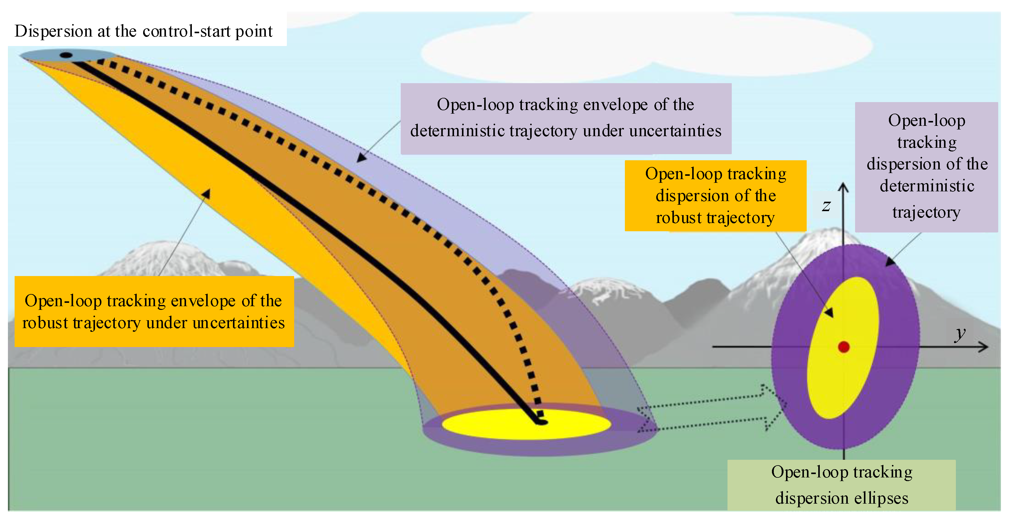
Figure 1. Schematic diagram of expected effect of open-loop robust planning for gliding trajectory.
Aerospace 11 00547 g001
Figure 2. Schematic diagram of the robust planning flow of gliding trajectory.
Aerospace 11 00547 g002
Figure 3. Uncertainty propagation results of gliding trajectory under specified control commands. (a) mean value of the velocity; (b) standard deviation of the velocity; (c) mean value of the inclination angle; (d) standard deviation of the inclination angle; (e) mean value of the deflection angle; (f) standard deviation of the deflection angle; (g) mean value of the flight time; (h) standard deviation of the flight time; (i) mean value of the altitude; (j) standard deviation of the altitude; (k) mean value of the lateral displacement; (l) standard deviation of the lateral displacement.
Aerospace 11 00547 g003aAerospace 11 00547 g003b
Figure 4. Open-loop robust planning results of gliding trajectory. (a) mean value of the velocity; (b) standard deviation of the velocity; (c) mean value of the inclination angle; (d) standard deviation of the inclination angle; (e) mean value of the deflection angle; (f) standard deviation of the deflection angle; (g) mean value of the flight time; (h) standard deviation of the flight time; (i) mean value of the altitude; (j) standard deviation of the altitude; (k) mean value of the lateral displacement; (l) standard deviation of the lateral displacement; (m) angle of attack; (n) angle of sideslip.
Aerospace 11 00547 g004aAerospace 11 00547 g004b
Figure 5. Closed-loop robust planning results of gliding trajectory. (a) velocity; (b) inclination angle; (c) deflection angle; (d) flight time; (e) altitude; (f) lateral displacement; (g) angle of attack; (h) angle of sideslip.
Aerospace 11 00547 g005
Figure 6. Tracking performance of the gliding projectile on the planned trajectory under different conditions: (a) altitude and (b) lateral displacement.
Aerospace 11 00547 g006
Figure 7. Open-loop tracking results of robust optimal control commands.
Aerospace 11 00547 g007
Table 1. Parameters related to the projectile and target.
ParameterValueParameterValueParameterValue
m   [ kg ] 44.5 C x 0 0.4 α max   [ ] 10
S   [ m 2 ] 0.0133 C y α 12 β max   [ ] 5
( x T , y T , z T )   [ km ] (40, 0, 10) k c 35 V f min   [ m s 1 ] 200
Table 2. Parameters related to uncertainties.
ParameterValueParameterValueParameterValue
σ d 0.0167 σ l 0.0167 σ l 0.0167
V 0   [ m s 1 ] 400 θ 0   [ ] 0 ψ 0   [ ] 0
σ V   [ m s 1 ] 20 σ θ   [ ] 2 σ ψ   [ ] 1
t 0   [ s ] 0 y 0   [ km ] 12.5 z 0   [ km ] 0
σ t   [ s ] 0.5 σ y   [ km ] 0.5 σ z   [ km ] 0.5
Table 3. Closed-loop guidance situations under different conditions in different scenarios.
ConditionScenario 1 Scenario 2 Scenario 3 Scenario 4
1×
2
3××××
4××
Table 4. Calculation times of single uncertainty propagation of the gliding trajectory using different methods.
Uncertainty Quantification MethodCalculation Time [s]
MCS45.69
Parallel MCS7.14
FOPCE1.46
COPCE0.23
Table 5. Values of each item in the closed-loop planning objective function in different scenarios.
Scenario ω D J o / J ¯ E c / E ¯ J c
100.95681.23061.2306
210.78441.45582.2402
350.55571.77154.5499
41000.48793.395152.1898
Disclaimer/Publisher’s Note: The statements, opinions and data contained in all publications are solely those of the individual author(s) and contributor(s) and not of MDPI and/or the editor(s). MDPI and/or the editor(s) disclaim responsibility for any injury to people or property resulting from any ideas, methods, instructions or products referred to in the content.