Abstract
Parasitic SAR formation can be flown at low altitude using smaller satellites and adding potential to conventional SAR mission From the orbital point of view, the main issue is related to the differential aerodynamic drag, which rapidly disrupts the formation. In this ambit, this paper proposes a case study of an along-track distributed parasitic receiver flying in formation with PLATiNO-1. Formation maintenance is the core contribution, highlighting how the active control of both altitude and in-plane anomalies leads to an unfeasible ΔV. Then, the active control of the altitude around the nominal value, which naturally controls anomaly shift, is proposed, modeled, and applied to the presented case study. It is shown that the annual ΔV can be reduced to the m/s range.
1. Introduction
After the first spaceborne Synthetic Aperture Radar (SAR) mission [1] was launched in 1978 based on the SeaSat satellite, a large satellite developed as a multi-sensor platform, the USA focused on the development of SAR payloads on board the Space Shuttle [2]. On the contrary, many other countries started long-lasting SAR satellite programs. Canada developed C-band Radarsat 1 [3], Radarsat 2 [4], and the three-satellite Radar Constellation Mission (RCM) [5], while Japan started its spaceborne L-band SAR program with JERS-1 [6] to further develop the ALOS program (ALOS-1 [7], ALOS-2 [8], ALOS-4 [9]). Europe developed a C-band SAR program through the European Space Agency (ESA) with the ERS-1/ERS-2 [10] and Envisat [11] satellites and the Sentinel-1 2-satellite constellation [12]. Later, Germany and Italy launched their national X-band SAR programs with the TerraSAR-X [13,14] and Tandem-X [15], Cosmo-SkyMed [16] and Cosmo Second Generation [17,18] constellation missions. Korea, India, and China later joined the group of countries who launched and operated SAR missions.
SAR missions have evolved in terms of both payload and satellite. Most of the former satellites were multi-payload spacecraft (e.g., ERS-1, J-ERS-1, Envisat). Then, the missions were optimized to fly SAR payloads only. The satellite mass initially increased, reaching the maximum of more than 8 tons with Envisat, then it was reduced (e.g., Sentinel-1, RCM). Nonetheless, almost all the cited missions have used large or very large spacecraft, with masses exceeding two tons in most cases. A few missions were developed and used smaller-mass spacecraft: the German military mission SAR-Lupe [19] and the Israelian TecSAR [20]. More recently, different approaches have been proposed and applied to SAR missions, strongly reducing the satellite mass to the microsatellite level. The Capella X-SAR program [21,22], initiated in 2016 by Capella Space to apply advanced antenna technology, was supported by a 100 kg mass spacecraft. The first demonstration mission was launched in 2018. The ICEYE Constellation [23,24] was developed by ICEYE, and was founded in 2014 as a spin-off of AaltoUniversity, Finland. ICEYE X2, the first operational satellite of the constellation, was launched at the end of 2018 on an 85 kg satellite.
When, at beginning of 2000, formation flying was proposed for the distribution of monolithic satellites over several smaller platforms, it was barely applied to SAR due to the cost of such missions. Thus, among the proposed distributed SAR studies [25], only Tandem-X was developed and operated as an SAR interferometer [15].
Although active SARs are under study for future along-track formation missions, a method to reduce the size and cost of SAR missions is the utilization of a passive-only radar designed to receive the signal transmitted by an active SAR (e.g., [26]). Such an approach can be extended by distributing the receiving-only radar over several smaller and simpler passive receivers. The parasitic signals are then combined by distributed aperture and beam forming processing techniques [27,28].
This paper is focused on an along-track receiving SAR formation, qualitatively described in Figure 1, where a standard transmitting/receiving SAR satellite is shown in red. The receiving-only companion is split over a number of smaller and lighter receiving-only SAR satellites, shown in blue. With respect to the standard bistatic configuration, with a single receiving satellite, the receiving-only channel has been fractionated. The fractionated nature of the receiver allows the system to both reduce the complexity (mass, volume, power consumption, data rate) of each parasitic item, and to enable new imaging modes depending on the technique utilized to combine and process the received signals. As an example, the receiving antenna in the along-track direction can be assembled by several received signals: the unambiguous azimuth signal can be recovered by interleaving the samples of different receivers working at a lower, ambiguous PRF. Otherwise, one could divide the along-track antenna aperture into multiple sub-apertures and perform interferometry and MTI at a lower resolution. The processing of samples has been explored in general in [27,28,29,30], while it was specifically addressed for along-track formation in [31,32,33,34].
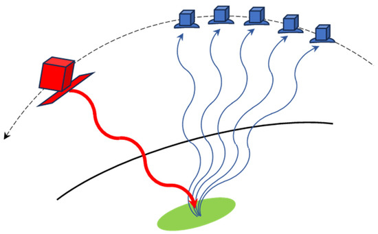
Figure 1.
Schematic of along-track fractionated formation.
It is worth noting that more compact satellites can be flown at a lower altitude where smaller antennas can take advantage of a shorter radar target range to compensate for the signal-to-noise ratio reduction caused by larger antenna apertures. Nonetheless, it was shown that the visibility time among active and passive radars can be a limitation when they are flown at different altitudes [35,36]. Thus, this paper will focus on a formation of a transmitting (Tx) SAR satellite and a parasitic, distributed companion flown at the same altitude. In particular, a study is performed to assess the capability to maintain the formation between the Tx SAR and the receiving-only (Rx) components in a low-orbital environment, where differential drag is the main cause of formation disruption. An analysis of an along-track formation is presented in Section 2, while the drag and critical aspects are discussed in Section 3. Formation maintenance is addressed in Section 4, where a novel maneuvering strategy is also proposed and modeled. The results refer to a parasitic formation operating in tandem with the Italian mission PLATiNO-1 [37,38] as the reference Tx X-band SAR.
2. Along-Track Formation Analysis
2.1. Overview of Formation Components
PLATiNO-1 [37,38] is the first mission in the PLATiNO program, developed to fly an X-band SAR payload. It is primarily designed to operate as a receiving-only radar when flying in tandem with Cosmo/Skymed or Cosmo Second Generation satellites (sun-synchronous orbit at 620 km altitude). It is also designed to operate as a classical transmitting/receiving SAR when its altitude is lowered to 410 km [37,38]. The PLATiNO-1 radar (3.125 cm wavelength) uses an antenna of 3.4 m × 0.75 m, a power consumption of 750 W (20 W in standby), and incidence angles between 20 deg and 40 deg. PLATINO has a launch mass of 200 kg (maximum) and an envelope with the dimensions 80 cm × 80 cm × 120 cm, which leads to a cross-section of approximately 1 m2. In addition, the satellite is equipped with electric propulsion for orbit maintenance.
This paper analyzes a receiving-only distributed train, which could be operated when PLATiNO-1 flies as a transmitting SAR at an altitude of 410 km. In particular, the train is operated in the along-track formation with PLATiNO-1. The distance between PLATiNO-1 and the receiving train is assumed to be 100 km, whereas the length of the receiving formation is assumed to be less than one kilometer.
With reference to the receiving-only element definition, some studies in the literature are particularly useful [39,40,41]. In the ambit of a NASA 6U-Cubesat mission to Mars, a high-gain antenna is studied [39]. Three different options are analyzed, including a deployable mesh reflector (0.5 m diameter, 1.4 kg mass). In a following study, a 1 m deployable mesh reflector antenna is proposed for X or Ka band communication [40], compatible with a 12U-class CubeSat (3U for antenna storage). A deployable paraboloid antenna is also proposed in [41], with a 1 m diameter, 8.3 cm height, focal length between 0.5 m and 0.75 m, and 3 kg mass. It is designed to be stored in a 3 Cubesat unit. For the scope of this paper, such an antenna is assumed as the reference receiving-only antenna to be flown on a 12U Cubesat. Main system parameters are listed in Table 1.

Table 1.
Main system parameters.
2.2. Tx/Rx Formation Analysis
In this section, some characteristics of the formation between PLATiNO-1 (the Tx element) and a single element (virtual Rx) are evaluated, assuming that the entire Rx formation collapses in its center. The orbital dynamics is simulated using Keplerian potential plus J2 secular perturbation using the mean anomaly, perigee anomaly, and ascending node right ascension.
Given the distance vector of this virtual Rx center with respect to the transmitter (baseline), its components are simulated in the orbiting reference of the transmitting satellite (origin in PLATiNO-1’s center of mass, z-axis directed along the local vertical, x-axis in the orbital plane and in the direction of motion, y-axis to complete the right-handed frame). It is worth underlining that the 100 km along-track separation corresponds to a difference in the argument of latitude Δu = 0.844° and to a time separation between the time of passage on the ascending node of 13.05 s.
Figure 2 shows that the baseline main component is primarily the along-track component, which oscillates around the 100 km value with an amplitude of about 100 m. Such oscillation is due to orbit eccentricity: an “elastic” effect between the two satellites tends to move them closer or further away depending on their angular distance from their respective perigees. This effect is extremely limited because the eccentricity is very small (order of magnitude 10−3). A vertical component is also present, with an oscillation around 750 m and amplitude of about 100 m, due to the fact that the satellites are not aligned but arranged along a curved trajectory. The cross-track component remains negligible along the whole orbit because the satellites share the same orbital plane.
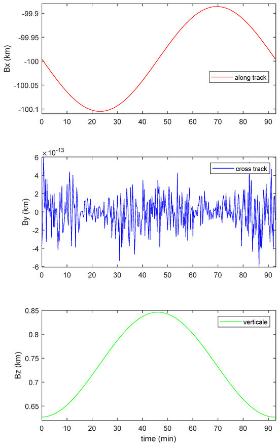
Figure 2.
Baseline components in the orbital reference frame in one period.
It is worth noting that these results agree with the model presented in [42], where it is shown that the offset is of the first order with respect to the differences in the orbital parameters, while the oscillation are second-order effects.
Rx antennas must observe in the direction of the illumination of the active radar satellite. Therefore, they should be pointed accordingly to the Tx satellite attitude, to Tx antenna pointing and to the baseline between the Tx and the Rx satellites (Figure 2). With reference to the Tx satellite attitude, SAR satellites typically perform a yaw steering maneuver to align the antenna with the direction of the satellite’s speed relative to the atmosphere, which minimizes the effects of aerodynamic resistance and, consequently, slows orbit decay. It is assumed that PLATiNO-1 performs this maneuver (Figure 3), which has the additional effect of almost nullifying the central Doppler frequency (ideally zero for a spherical Earth and circular orbit) in the monostatic image. As for the PLATiNO-1 antenna pointing, it is worth remembering that it can be pointed in elevation with angles between 20 deg and 40 deg.
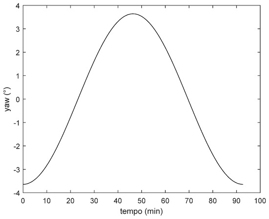
Figure 3.
Yaw attitude angle (yaw steering maneuver) of Tx satellite along one orbit.
A study of the Rx satellite attitude was performed by the authors of [43], with application to a cross-track bistatic SAR configuration. The approach relied on a roll–pitch–yaw attitude sequence, assuming that the antenna is mounted with its boresight aligned with the local vertical. The roll and pitch of the Rx satellite let the boresight of the Rx antenna point towards the Earth, illuminated by the boresight of the Tx antenna (swath centers coincide). Then, the yaw angle aligns with the cross-track direction of the Rx and Tx radars. While the roll and pitch are mandatory, the yaw is optional (depending on 3 dB swath angles, processing, etc.). Since the model developed in [43] had a general geometrical and analytical approach, it can be applied to the present case of an along-track formation.
Figure 4 shows the trends of the roll, pitch, and yaw of Rx satellites. Required roll angles are almost constant and in practice coincide with the elevation angles of the transmitting radar. The required pitch angle is instead linked to the need to chase a radar that is further ahead and corresponds to an oscillation at an orbital frequency of a few degrees. The pitch angle mean value decreases with the Tx elevation angle, because the larger the Tx elevation, the closer the Tx beam center and Rx elevation direction are. The yaw angle instead increases with the elevation angle of the transmitting radar.
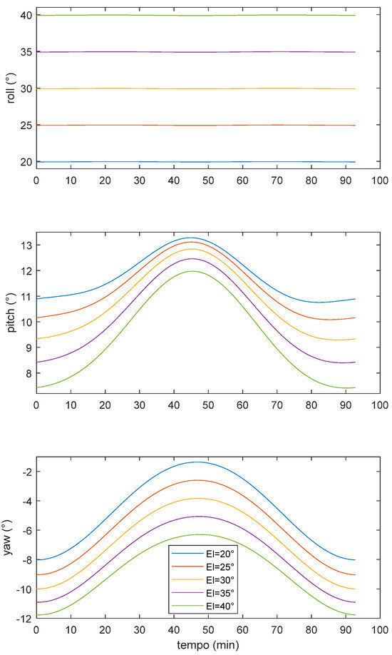
Figure 4.
Pointing angles of Rx satellites along one orbit.
If the Rx antennas are mounted with their boresights oriented towards the mean values of the expected oscillations (Figure 4), the expected excursions of the Rx angular oscillations can be limited. Such oscillations can then be obtained by either a satellite attitude maneuver by an equivalent antenna pointing (mechanical or electronical). Finally, while the roll and pitch are essential to attain overlap between the Tx and Rx swath centers, the yaw can be considered optional.
2.3. A Note on Rx Formation
Rx elements are in close formation. As an example, consider a formation of five elements at 200 m distance for a total formation extension of 800 m in an along-track formation. To attain this along-track cluster, satellites are to be distributed over the same Tx orbit with a mean anomaly shift corresponding to the nominal satellite distance (1.7 × 10⁻³ deg). Since the orbit of the Tx is elliptical, one must expect an oscillation of this distance along the orbit. This oscillation will be of a small amplitude since the eccentricity of the transmitter is small. The separation between the successive satellites oscillates around the nominal value of 200 m with an amplitude of approximately 22 cm (Figure 5). The overall length of the formation also oscillates with an amplitude of approximately 88 cm around the nominal value of 800 m. In both cases, the amplitude of the oscillation is 0.1% of the nominal value; therefore, it does not pose safety problems for the satellites, at least in the nominal condition, since a drift in general will be observed due to secondary factors not yet included.
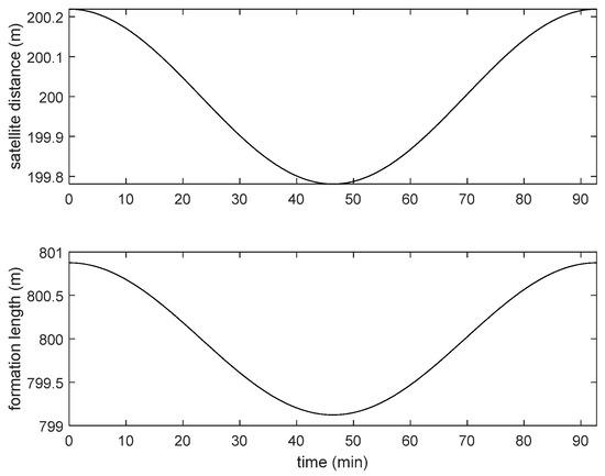
Figure 5.
Rx formation distances along an orbit.
3. Evaluation of Drag Effects and Criticalities
3.1. Drag Perturbation Overview
Apart from the J2 secular perturbations, additional geopotential harmonics (three orders of magnitude smaller than J2) are typically considered in numerical simulations, while it is quite complex to include them in design-oriented analytical models. In addition, it is worth noting that all satellites share the same orbital parameters, with the only difference in the mean anomaly (less than 1 deg). Thus, it is expected that additional harmonics of the Earth’s geopotential equally (or practically equally) affect all the satellites with a minor impact on the relative motion. With reference to the three-body attraction in LEO, it is typically an order of magnitude smaller than the J2 potential. In terms of the differential contribution, it should be negligible because all the satellites share the same nominal altitude and orbital plane. Finally, the main contribution of the solar radiation pressure consists of an eccentricity oscillation, which is also very difficult to model without precise satellite geometry and surface characteristics.
Thus, the main issue in formation control is related to drag. If we consider Rx satellites, it must be noted that they have the same design; thus, they have the same shape, volume, and mass. The nominal ballistic coefficient is the same. In addition, they are very close to one another, which means that they fly at very close anomalies. Therefore, the aerodynamic drag affects all the Rx satellites to the same extent.
On the contrary, the Tx satellite has an independent design. Therefore, it can be expected that it performs better with respect to the drag (bigger satellites typically attain a better mass-to-area ratio). In addition, since bigger satellites have more platform resources, one can imagine that its propulsion capability exceeds those of the Rx satellites. Regarding PLATiNO-1 specifically, orbit control relies on an electrical propulsion subsystem. With all these considerations in mind, it is assumed that PLATiNO-1 follows its nominal trajectory, while the Rx satellites should control their relative geometry with respect to the transmitter. To evaluate how the relative geometry varies and hypothesize the necessary corrective maneuvers to restore the desired configuration, consider the mean semimajor axis reduction:
which also impacts the perturbed mean motion and secular precession rate of the ascending node:
where ρ is the atmospheric density, CD is the satellite drag coefficient, A is the satellite cross-section, m is the satellite mass, a is the orbit semimajor axis, M is the satellite mean anomaly, is the nominal mean motion, Ω is the ascending node right ascension, and is the nominal ascending node precession rate. Therefore, three effects should be considered: the altitude reduction, reduction in the along-track separation, and rotation of the orbital plane. To quantify such effects, it is necessary to evaluate the ballistic coefficient, CDA/m. The mass can be budgeted at 15 kg, considering 12 kg for the bus (12U Cubesat) and 3 kg for the deployable antenna [41]. With reference to cross-section A, a 12U Cubesat can be arranged in different configurations. Three possible configurations are considered (Figure 6), while other options with more elongated figures are discarded because they could pose difficulties in components and subsystem arrangements. We also consider the deployable solar array on the surfaces lying in the orbital plane, because PLATiNO-1′s ascending node local time is 5:45 am.
In particular, if the area of a face of a standard Cubesat is given as A = 10 cm × 10 cm, the velocity frontal area (Af) is given as 3A, 4A, and 6A for the three considered configurations. The lateral areas (Al) are instead 12A, 12A, and 6A, respectively. Asa is 24A for configurations (a) and (b), and 12A for configuration (c). Thus, the satellite cross-section can be estimated as
which stands if the satellite does not perform a yaw maneuver and where γ is the angle which would be necessary to align the satellite x-axis with the satellite–atmosphere relative velocity (order of a few degrees, Figure 3). Since γ is small, one can expect that configuration (a) (with the smaller Af) should be the one which minimizes the cross-section. Figure 7 shows the satellite cross-section for the three analyzed configurations along a whole orbit. Their mean values are 445 cm2 (a), 545 cm2 (b), and 672 cm2 (c).
With reference to the antenna cross-section, it is a circular segment with an 8.3 cm height and 1 m chord () when the antenna is pointed towards the local vertical. When the Rx antenna is operating it must be oriented accordingly to the roll and pitch angles in Figure 4. While the roll does not cause any effects, the pitch has a significant impact because antenna cross section is now related the area of a 1 m diameter circle (Ac):
For a mean pitch angle of 10.5°, we obtain . It is assumed that the pitch angle is applied only during image acquisition, and thus is limited to the Rx radar duty cycle to reduce the attitude maneuver effort and antenna cross-section. If a 5% duty cycle is assumed for the Rx radars, the mean antenna cross-section can be estimated at 602 cm2. Thus, we obtain an overall cross-section of 1047 cm2 (a), 1147 cm2 (b), and 1274 cm2 (c).
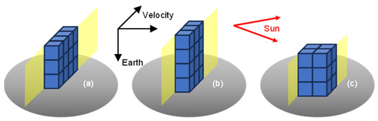
Figure 6.
Considered candidate geometries for a 12U Cubesat.
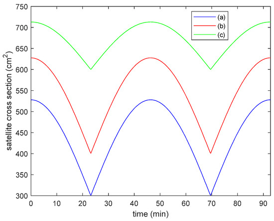
Figure 7.
Satellite cross-section for the three configurations along an orbit.
3.2. Maintenance Preliminary Analysis
Considering the three configurations in Figure 6a,b are almost equivalent from a geometrical point of view and from the perspective of solar array extension, but Figure 6b has a worse cross-sectional area, the configuration in Figure 6c would offer more flexibility in subsystem allocation, center of mass, and moment of inertia optimization, but it implies the largest cross-sectional area. In addition, the configuration in Figure 6c halves the solar array area, unless a more complex, multi-surface deployment system is considered. Therefore, the configuration in Figure 6a is selected to evaluate the maintenance efforts. Considering the evaluated cross-sectional area, satellite mass of 15 kg, and assuming a drag coefficient of 2.2, we obtain a ballistic coefficient of 1.54 × 10⁻² m2/kg.
Remembering that the Tx satellite is considered on its nominal orbit because it is equipped with electrical propulsion, the effects of aerodynamic resistance (Equation (1)) lead to a relative orbital decay (Figure 8) estimated at about 11.6 km in one year if no orbital control is applied. The critical issue of orbital decay is related to the along-track drift, which is induced by an altitude difference (Equation (2)). Figure 9 shows that the Rx satellites, flying at a decreasing altitude, would proceed faster than the Tx satellite, and in less than one week, they would nullify the nominal 100 km along-track separation.
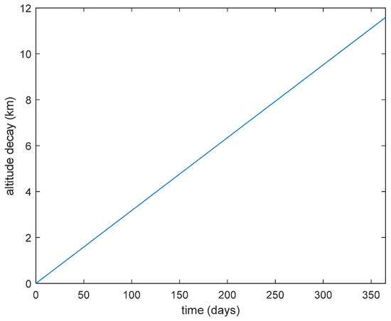
Figure 8.
Altitude decay of Rx satellite in one year.
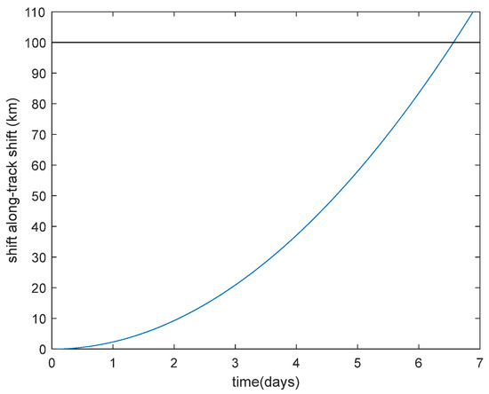
Figure 9.
Along-track shift of Rx with respect to PLATiNO-1 satellites in 7 days.
The results show that Rx orbital control is mandatory. If it is approached through controlling both the altitude and along-track shift, the three-pulse orbit maneuver presented in [26] can be used (Table 2). Just as a limiting and inapplicable case, imagine that the control maneuver is applied when the Rx satellite has totally nullified the 100 km along-track offset. The first column of Table 2 shows that each maneuver requires a speed variation of about 12 m/s and an unfeasible annual budget for this satellite class.
Table 2.
Maneuver results.
If about 6.6 days occur before applying orbital control, growth is allowed to become exponential (Figure 9) and its effects are demanding. Therefore, as a second example, the orbit maneuver is applied after 1 day (second column in Table 2) when the altitude has decayed less and, above all, the along-track drift is still following a linear pattern. The beneficial effects of reducing the time between maneuvers are clear. The reduction in ΔV per maneuver is so large that it overcompensates for the increase in the number of required maneuvers. The ΔV per year decreases by a factor of more than 6. Nevertheless, such a ΔV budget is still not compatible with the 12U Cubsat’s typical resources.
It is worth noting that the maneuver time is the time that the satellite spends on the transfer orbits, which, for the maneuver utilized in Table 2, is composed of two arcs of elliptic orbits (as described in [26]). Since this time likely corresponds to satellite unavailability, it can become an additional critical element if the maneuver frequency is increased.
It is worth underlining that the critical element of the considered maneuver is anomaly correction: if the altitude decay is corrected only, a Hohmann transfer with ΔV = 1.177 × 10⁻¹ m/s (1.792 × 10⁻² m/s) per maneuver is computed for Δh = 208.5 m (31.75 m). Therefore, for the Rx satellites to feasibly fly in formation with PLATiNO-1, a different control strategy is needed with a different approach to along-track separation management.
4. Formation Maintenance: Modeling and Results
4.1. Maintenance Concept and Modeling
A maneuver strategy is proposed to compensate for the orbital decay due to the atmospheric drag without the need to correct for in-plane anomaly shifts. Let us refer to Figure 10, where the nominal, circular orbit of radius aC is highlighted in blue and the nominal satellite position is identified by the blue circle (clockwise orbital motion). Let us suppose that the satellite is initially placed on a circular orbit at an altitude higher than the nominal one (green circumference, semimajor axis aC + Δh) and at the same argument of latitude in order to have the nominal (blue circle) and the real (black square) satellites initially aligned along the local vertical.
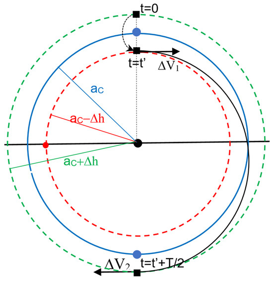
Figure 10.
Orbits and maneuver strategy.
Therefore, under an orbital environment perturbed by atmospheric drag, the satellite will start decaying. With respect to the nominal, unperturbed counterpart, it exhibits an altitude reduction and an anomaly shift. Such a shift is backward at any semimajor axis a > aC, whereas it is forward when a < aC. Thus, it is expected that the maximum backward shift is reached when the satellite is at the nominal radius aC. When, at time t’, the real satellite has reached the semimajor axis aC − Δh, we will demonstrate that the anomaly shift has been compensated for in the first order. Thus, the real satellite is placed on a decayed orbit (red circumference, semimajor axis aC − Δh) but again aligned with the nominal satellite along the local vertical: during the altitude reduction 2Δh, the satellite will shift backwards and forwards with an overall ΔM = 0.
To analyze the proposed orbit/maneuver strategy, let us propose a power expansion in the first order of the semimajor axis, considering that a is of the order of thousands of kilometers (LEO) and Δh is of the order of tens of meters (Δh/aC is of the order of 10−6). Time t0 (set conventionally at 0) represents the time instant when the satellite is orbiting on a circular orbit at aC + Δh and is aligned with the virtual one and Δa = Δh. Thus, with Δh/aC « 1,
Under the same assumptions, the mean motion difference can be derived and the mean anomaly relative shift can be evaluated:
Therefore, if t’ is the time when the altitude has decayed by 2Δh, we obtain
Substituting Equation (9) into Equation (8), it results in that when the satellite is decayed by 2Δh, it is also aligned with its virtual counterpart (ΔM(t’) = 0).
When the satellite is decayed by 2Δh, the initial altitude can be attained by a Hohmann transfer with perigee aC − Δh and apogee aC + Δh. Since the Hohmann trajectory and nominal orbit share the same semimajor axis and period, the maneuver does not add any ΔM.
4.2. Application and Results
The model is applied to Rx satellites and PLATiNO-1, considering a different number of days between successive maneuvers, which has been varied between 1 and 10. Figure 11 shows the initial altitude difference necessary to perform the proposed maneuver. It varies linearly from a minimum of about 15.9 m to a maximum of about 159 m.
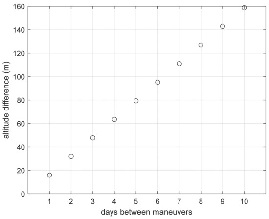
Figure 11.
Initial altitude difference as a function of time between maneuvers.
The maximum along-track drift with respect to the nominal Rx satellite (Figure 12) also increases with the time interval between maneuvers from about 580 m (1 day) to about 58 km (10 days). The along-track shift is not linear, but rapidly increases with time.
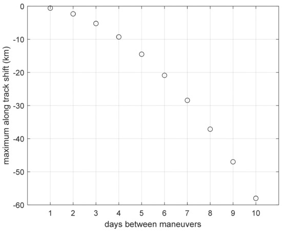
Figure 12.
Maximum along-track shift as a function of time between maneuvers.
Finally, Figure 13 shows that the single velocity pulses are of the order of a few centimeters and are almost equal, which is expected because the lower and higher orbits are very close. Thus, each maneuver weighs less than 20 cm/s, varying from 1.79 cm/s to 17.9 cm/s. The annual budget for ΔV is around 6.6 m/s for any options, with oscillations related to integer truncation to determine the number of maneuvers per year.
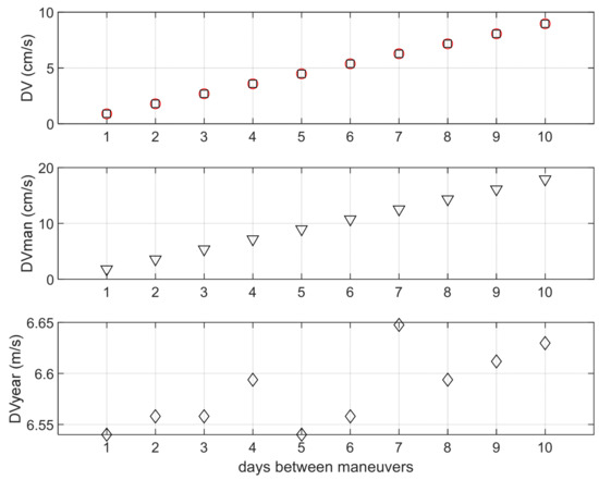
Figure 13.
ΔV budget as a function of time between maneuvers.
The different options are equivalent in practice from the point of view of the ΔV budget, but they can be selected considering the total number of annual maneuvers and the along-track drift. Less maneuvers mean less interruptions of satellite operations but a larger drift, which causes a larger variation in the radar bistatic angle. The 5-day maneuver is selected.
To highlight the maneuver’s peculiarities, a simulation has been carried out considering a non-linearized semimajor axis variation for the 5-day option (Figure 14). This requires an initial altitude difference of 79.4 m (upward), which reduces to zero after 2.5 days to increase to 79.4 (downward) at 5 days. The along-track drift varies from 0 (initial nominal condition) to a backward maximum of 14.5 km, attained at 2.5 days, to return to 0 at 5 days. Both these results are in full agreement with the linearized model, which confirms that the selected option meets the condition of the validity of the linearization.
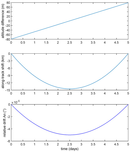
Figure 14.
Relative motion drifts during the 5 days between maneuvers.
The relative drift of the Tx and Rx ascending nodes is also simulated. It is worth underlining that the altitude variation above and below the nominal value has an additional and beneficial effect on the formation maintenance. The node drifts backward for half the period, to advance again for the second half. Thus, there is no need to correct the node drift. The only ΔV to be budgeted is 6.54 m/s per year, which confirms the validity of the maneuver approach proposed in Section 4.1.
5. Conclusions
This paper has analyzed a parasitic formation of 12U Cubesat satellites which integrate an Rx-only SAR designed to receive the signal transmitted by PLATiNO-1, an SAR satellite flying in an almost circular orbit at a 410 km altitude. In particular, the analysis has dealt with an attitude and orbital analysis.
The Rx satellites fly in an along-track formation with PLATiNO-1, with the same orbital parameters but a mean anomaly that is different to guarantee adequate along-track separation. The results show that the Rx satellites need to point their line-of-sight, either electronically or mechanically, to superimpose their antenna swath with the Tx one. Roll and pitch pointing is mandatory. The required roll for the Rx satellite/antenna is very close to the transmitter elevation angle, while the pitch is an oscillation of a few degrees, always within 7° and 14°. The yaw is optional and it consists of an oscillation of about 6°, always within the range between −1° and −12°.
The main orbital issue is related to formation maintenance to counteract differential drag, which mainly acts on along-track separation. To this end, an analysis has been performed to estimate the satellite cross-section on the basis of attitude and pointing. Then, it has been shown that a control approach designed to periodically correct for both altitude and along-track separation variation and to transfer the Rx satellites in their nominal position is unfeasible. Such maneuvers, in fact, foresee a ΔV budget per year of more than 100 m/s, which is largely incompatible with a 12U Cubesat.
Finally, a maneuver concept has been proposed and modeled, which consists of flying Rx satellites around the nominal orbit with oscillations in both altitude and along-track separation. Such an approach allows one to counteract for the altitude only, because the anomaly shift is naturally compensated for by the orbital decay. A maneuver of altitude variation has been proposed that is repeated every 5 days, which controls the altitude in an overall variation of less than 160 m around the nominal value of 410 km. The along-track separation increases by slightly less than 15 km to naturally return to its nominal value. The annual cost of the maintenance maneuver is lowered by two orders of magnitude, reducing to about 6.5 m/s.
Funding
This research was funded in part by the Italian Ministry of University and Research (MIUR) in the ambit of the Project ARS01_00922 in the framework of PNR 2015–2020.
Data Availability Statement
The data supporting the conclusions of this article consist of simulations which are graphically reported in the figures. The numerical data from the simulations will be made available by the authors on request.
Conflicts of Interest
The author declares no conflicts of interest.
References
- Jordan, R.L. The Seasat-A Synthetic Aperture Radar System. IEEE J. Ocean. Eng. 1980, OE-5, 154–164. [Google Scholar] [CrossRef]
- Way, J.B.; Atwood Smith, E.L. The Evolution of Synthetic Aperture Radar Systems and their Progression to the EOS SAR. IEEE Trans. Geosci. Remote Sens. 1991, 29, 962. [Google Scholar] [CrossRef]
- Mahmood, A. RADARSAT-1 Background Mission for a global SAR coverage. In Proceedings of the IEEE International Geoscience and Remote Sensing Symposium, Singapore, 3–8 August 1997. [Google Scholar]
- Morena, L.C.; James, K.V.; Beck, J. An introduction to the RADARSAT-2 mission. Can. J. Remote Sens. 2004, 30, 221–234. [Google Scholar] [CrossRef]
- Cote, S.; Lapointe, M.; De Lisle, D.; Arsenault, E.; Wierus, M. The RADARSAT Constellation: Mission Overview and Status. In Proceedings of the 13th European Conference on Synthetic Aperture Radar, Online, 29 March–1 April 2021. [Google Scholar]
- Nemoto, Y.; Nishino, H.; Ono, M.; Mizutamari, H.; Nishikawa, K.; Tanaka, K. Japanese Earth Resources Satellite-1 Synthetic Aperture Radar. Proc. IEEE 1991, 79, 800–809. [Google Scholar] [CrossRef]
- Rosenqvist, A.; Shimada, M.; Ito, N.; Watanabe, M. ALOS PALSAR: A Pathfinder Mission for Global-Scale Monitoring of the Environment. IEEE Trans. Geosci. Remote Sens. 2007, 45, 3307–3316. [Google Scholar] [CrossRef]
- Kankaku, Y.; Suzuki, S.; Osawa, Y. ALOS-2 mission and development status. In Proceedings of the IEEE International Geoscience and Remote Sensing Symposium, Melbourne, Australia, 21–26 July 2013. [Google Scholar]
- Motohka, T.; Kankaku, Y.; Miura, S.; Suzuki, S. Alos-4 L-Band SAR Mission and Observation. In Proceedings of the IEEE International Geoscience and Remote Sensing Symposium, Yokohama, Japan, 28 July–2 August 2019. [Google Scholar]
- Attema, E. The Active Microwave Instrument On-Board the ERS-1 Satellite. IEEE Proc. 1991, 79, 791–799. [Google Scholar] [CrossRef]
- Louet, J. The Envisat Mission and System. ESA Bull. 2001, 106, 10–25. [Google Scholar]
- Attema, E.; Bargellini, B.; Edwards, P.; Levrini, G.; Lokas, S.; Moeller, L.; Rosich-Tell, B.; Secchi, P.; Torres, R.; Davidson, M.; et al. Sentinel-1—The Radar Mission for GMES Operational Land and Sea Services. ESA Bull. 2007, 131, 10–17. [Google Scholar]
- Werninghaus, R.; Buckreuss, S. The TerraSAR-X Mission and System Design. IEEE Trans. Geosci. Remote Sens. 2010, 48, 606–614. [Google Scholar] [CrossRef]
- Pitz, W.; Miller, D. The TerraSAR-X Satellite. IEEE Trans. Geosci. Remote Sens. 2010, 48, 615–621. [Google Scholar] [CrossRef]
- Krieger, G.; Papathanassiou, K.P.; Younis, M. Interferometric Synthetic Aperture Radar (SAR) Missions Employing Formation Flying. Proc. IEEE 2010, 98, 816–843. [Google Scholar] [CrossRef]
- Caltagirone, F. Status, results and perspectives of the Italian Earth Observation SAR COSMO–SkyMed. In Proceedings of the European Radar Conference, Rome, Italy, 30 September–2 October 2009. [Google Scholar]
- Calabrese, D.; Croce, A.; Spera, G.; Venturini, R.; De Luca, G.F.; Serva, S. COSMO SG, System Overview and Performance. In Proceedings of the 10th European Conference on Synthetic Aperture Radar, Berlin, Germany, 2–6 June 2014. [Google Scholar]
- Scorzafava, E.; Monaci, F.; Zampolini Faustini, E.; L’Abbate, M.; Capece, P.; Lumaca, F.; Campolo, G.; Panetti, A.; Spera, G.; Pavia, P.; et al. COSMO SG, Spacecraft design and technological challenge. In Proceedings of the 10th European Conference on Synthetic Aperture Radar, Wessling, Germany, 2–6 June 2014. [Google Scholar]
- eoPortal. Available online: http://directory.eoportal.org/pres_SARLupeConstellation.html (accessed on 18 June 2024).
- Naftaly, U.; Levy-Nathansohn, R. Overview of the TECSAR Satellite Hardware and Mosaic Mode. IEEE Geosci. Remote Sens. Lett. 2008, 5, 423–426. [Google Scholar] [CrossRef]
- eoPortal. Available online: https://www.eoportal.org/satellite-missions/capella-x-sar (accessed on 18 June 2024).
- Farquharson, G.; Woods, W.; Stringham, C.; Sankarambadi, N.; Riggi, L. The Capella Synthetic Aperture Radar Constellation. In Proceedings of the IEEE International Geoscience and Remote Sensing Symposium, Valencia, Spain, 22–27 July 2018. [Google Scholar]
- eoPortal. Available online: https://www.eoportal.org/satellite-missions/iceye-constellation (accessed on 18 June 2024).
- Ignatenko, V.; Laurila, P.; Radius, A.; Lamentowski, L.; Antropov, O.; Muff, D. ICEYE Microsatellite SAR Constellation Status Update: Evaluation of First Commercial Imaging Modes. In Proceedings of the IEEE International Geoscience and Remote Sensing Symposium, Waikoloa, HI, USA, 26 September–2 October 2020. [Google Scholar]
- D’Errico, M. (Ed.) Distributed Space Missions for Earth System Monitoring; Springer: New York, NY, USA, 2013; pp. 375–545. [Google Scholar]
- D’Errico, M.; Grassi, M.; Vetrella, S. A Bistatic SAR Mission for Earth Observation based on a Small Satellite. Acta Astronaut. 1996, 39, 837–846. [Google Scholar] [CrossRef]
- Goodman, N.A.; Stiles, J.M. Resolution and synthetic aperture characterization of sparse radar arrays. IEEE Trans. Aerosp. Electron. Syst. 2003, 39, 921–935. [Google Scholar] [CrossRef]
- Younis, M.; Fischer, C.; Wiesbeck, W. Digital beamforming in SAR systems. IEEE Trans. Geosci. Remote Sens. 2003, 41, 1735–1739. [Google Scholar] [CrossRef]
- Goodman, N.A.; Chung Lin, S.; Rajakrishna, D.; Stiles, J.M. Processing of multiple-receiver spaceborne arrays for wide-area SAR. IEEE Trans. Geosci. Remote Sens. 2002, 40, 841–852. [Google Scholar] [CrossRef]
- Krieger, G.; Moreira, A. Spaceborne bi- and multistatic SAR: Potential and challenges. IEE Proc. Radar Sonar Navig. 2006, 153, 184–198. [Google Scholar] [CrossRef]
- Sakar, N.; Rodriguez-Cassola, M.; Prats-Iraola, P.; Moreira, A. Azimuth reconstruction algorithm for multistatic SAR formations with large along-track baselines. IEEE Trans. Geosci. Remote Sens. 2020, 58, 1931–1940. [Google Scholar] [CrossRef]
- Renga, A.; Graziano, M.D.; Moccia, A. Formation Flying SAR: Analysis of Imaging Performance by Array Theory. IEEE Trans. Aerosp. Electron. Syst. 2021, 57, 1480–1497. [Google Scholar] [CrossRef]
- Di Martino, G.; Di Simone, A.; Iodice, A.; Riccio, D.; Ruello, G. Efficient Processing for Far-From-Transmitter Formation-Flying SAR Receivers. IEEE Trans. Geosci. Remote Sens. 2023, 61, 1–19. [Google Scholar] [CrossRef]
- Renga, A.; Gigantino, A.; Graziano, M.D. Multiplatform Image Synthesis for Distributed Synthetic Aperture Radar in Long Baseline Bistatic Configurations. IEEE Trans. Aerosp. Electron. Syst. 2023, 59, 9267–9284. [Google Scholar] [CrossRef]
- Sarno, S.; Graziano, M.D.; Fasano, G.; D’Errico, M. Very-Low Altitude Parasitic Radar Distributed on Small Satellites. Adv. Space Res. 2018, 62, 3462–3474. [Google Scholar] [CrossRef]
- Sarno, S.; Fasano, G.; D’Errico, M. Modeling Relative Motion of LEO Satellites at Different Altitudes. Acta Astronaut. 2020, 156, 197–207. [Google Scholar] [CrossRef]
- eoPortal. Available online: https://www.eoportal.org/satellite-missions/platino (accessed on 20 June 2024).
- Sabbatinelli, B.; Stanzione, V.; Cicic, A.; Molina, M.; Calà, E.; Longo, F.; Formaro, R. PLATiNO Project: A new Italian multi-application small satellite platform for highly competitive missions. In Proceedings of the 69th International Astronautical Congress, Bremen, Germany, 1–5 October 2018. [Google Scholar]
- Hodges, R.E.; Chahat, N.; Hoppe, D.J.; Vacchione, J.D. A Deployable High-Gain Antenna Bound for Mars: Developing a new folded-panel reflectarray for the first CubeSat mission to Mars. IEEE Antennas Propag. Mag. 2017, 59, 39–49. [Google Scholar] [CrossRef]
- Chahat, N.; Sauder, J.; Mitchell, M.; Beidleman, N.; Freebury, G. One-Meter Deployable Mesh Reflector for Deep-Space Network Telecommunication at X-Band and Ka-Band. IEEE Trans. Antennas Propag. 2020, 68, 727–735. [Google Scholar] [CrossRef]
- Di Martino, G.; Di Simone, A.; Grassi, M.; Grasso MGraziano, M.D.; Iodice, A.; Moccia, A.; Renga, A.; Riccio, D.; Ruello, G. Formation-Flying SAR Receivers in FAR-from-Transmitter Geometry: X-Band SAR Antenna Design. In Proceedings of the IEEE International Geoscience and Remote Sensing Symposium IGARSS, Brussels, Belgium, 11–16 July 2021. [Google Scholar]
- Fasano, G.; D’Errico, M. Modeling Orbital Relative Motion to Enable Formation Design from Application Requirements. Celest. Mech. Dyn. Astron. 2009, 105, 113–139. [Google Scholar] [CrossRef]
- D’Errico, M.; Moccia, A. Attitude and Antenna Pointing Design of Bistatic Radar Formations. IEEE Trans. Aerosp. Electron. Syst. 2003, 39, 949–960. [Google Scholar] [CrossRef]
Disclaimer/Publisher’s Note: The statements, opinions and data contained in all publications are solely those of the individual author(s) and contributor(s) and not of MDPI and/or the editor(s). MDPI and/or the editor(s) disclaim responsibility for any injury to people or property resulting from any ideas, methods, instructions or products referred to in the content. |
© 2024 by the author. Licensee MDPI, Basel, Switzerland. This article is an open access article distributed under the terms and conditions of the Creative Commons Attribution (CC BY) license (https://creativecommons.org/licenses/by/4.0/).