
Brushless DC Motor Sizing Algorithm for Small UAS Conceptual Designers


Abstract
:1. Introduction
1.1. Motor Primer
- 1.
- 2.
- Winding resistance () is, as the name implies, the resistance of the motor’s windings to the current flow. The winding resistance is roughly analogous to an aerodynamic body’s parasitic drag coefficient ().
- 3.
- Motor figure of merit () quantifies how well a particular motor’s design converts current into torque rather than copper losses (), as defined in Equation (3). The figure of merit is roughly analogous to a wing’s lift-to-drag coefficient ().
1.2. Literature Review
2. Methodology
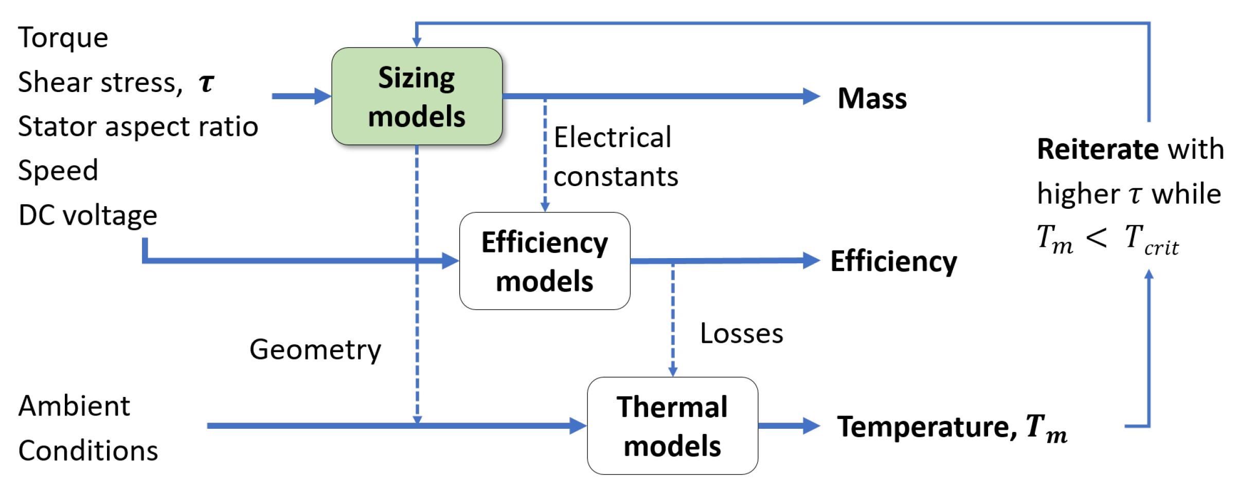
2.1. Overall Algorithm
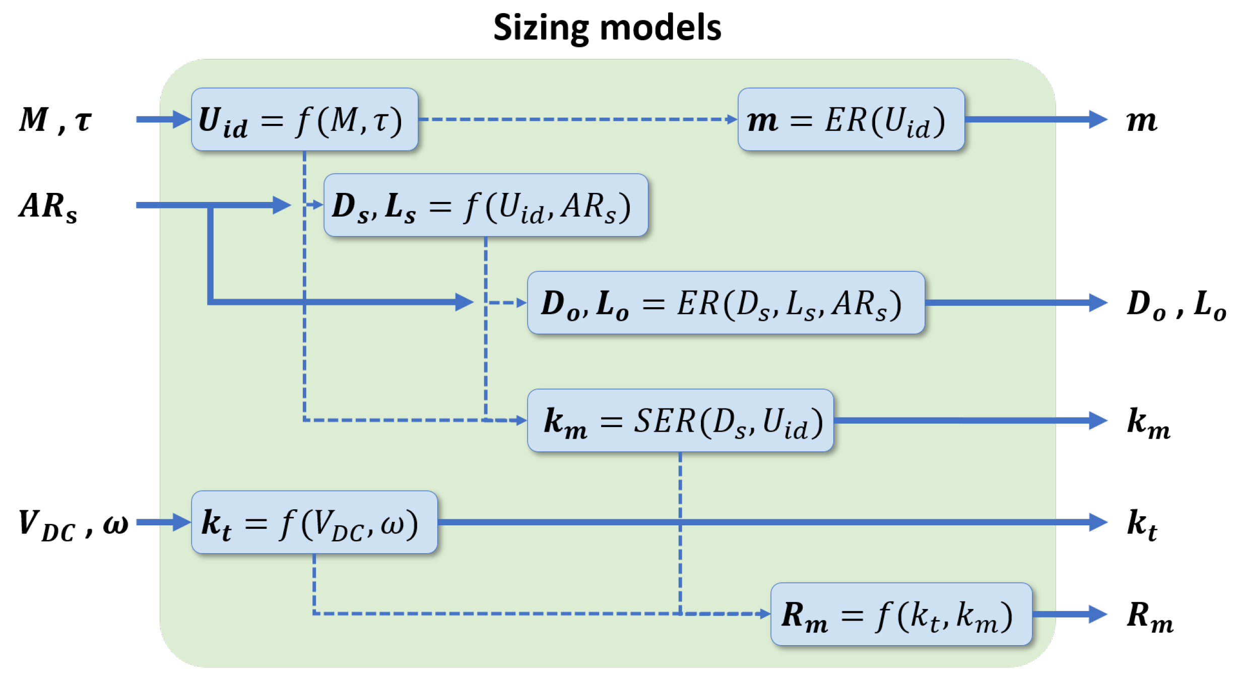
2.2. Sizing Models
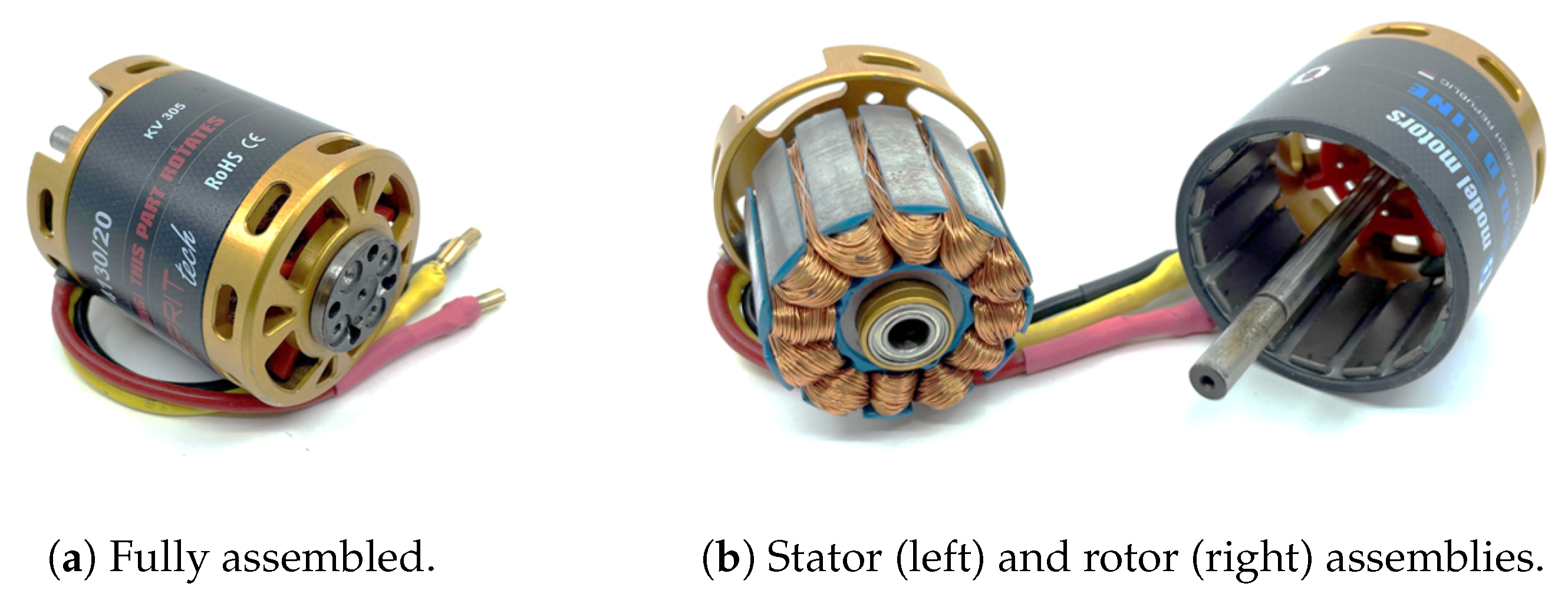
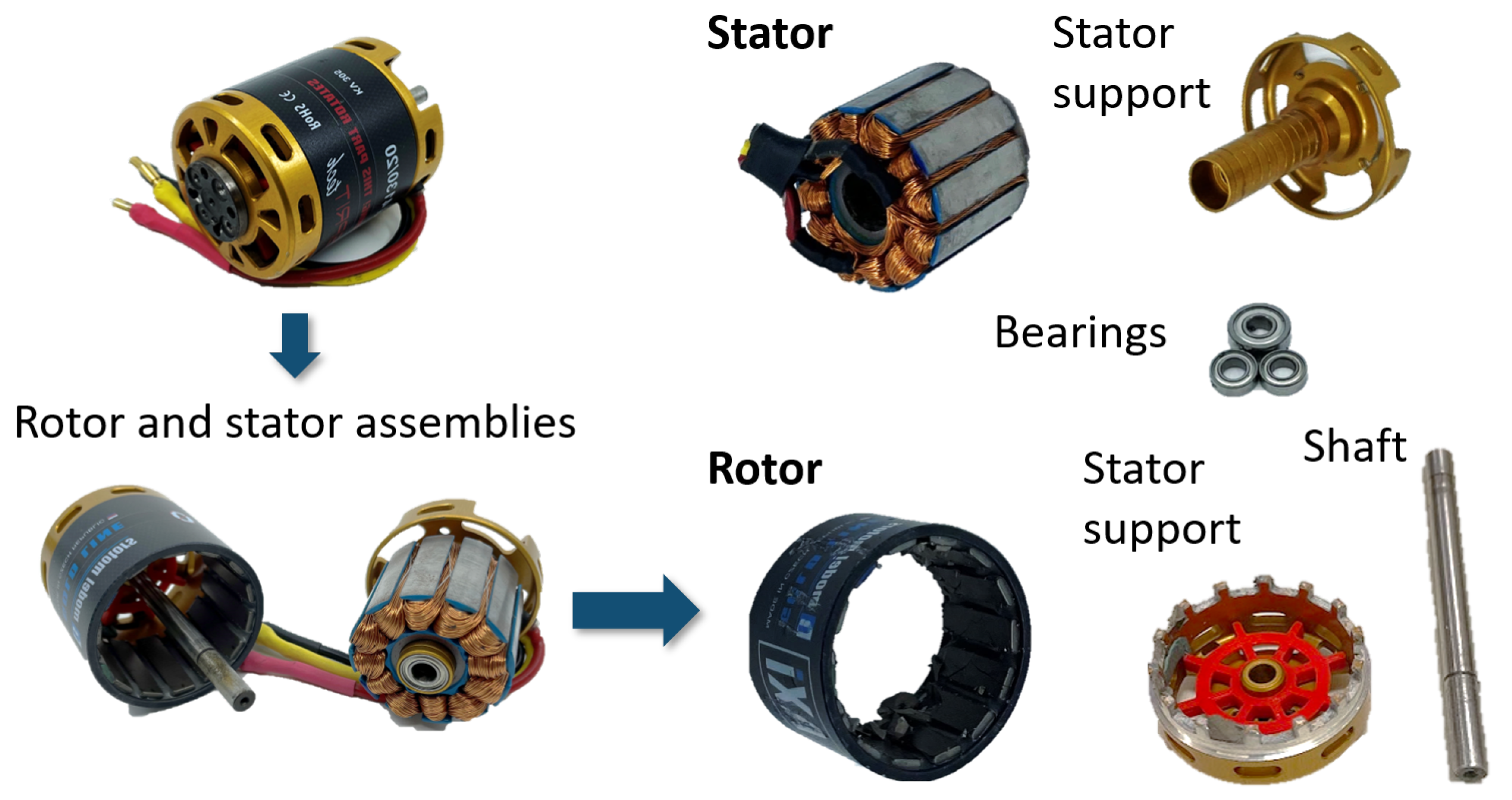
2.3. Teardown Motors
3. Teardown and Analysis
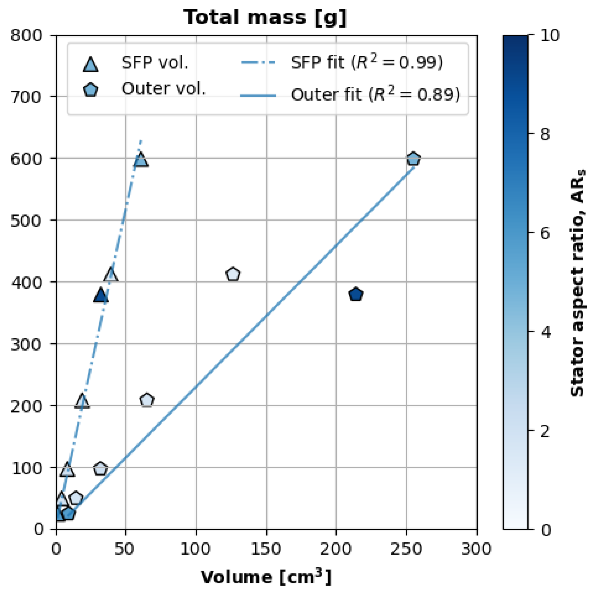
3.1. Mass Trends
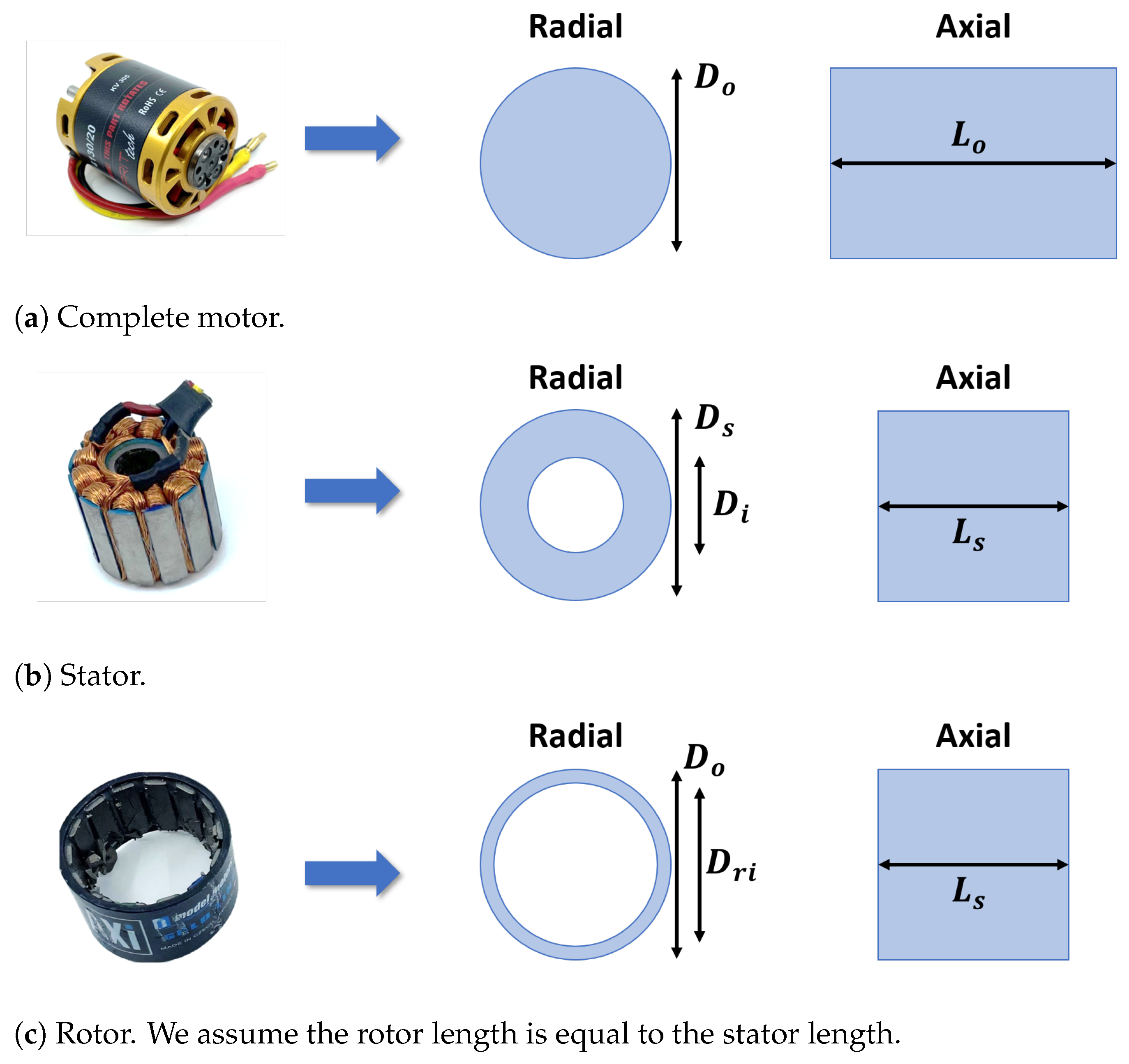
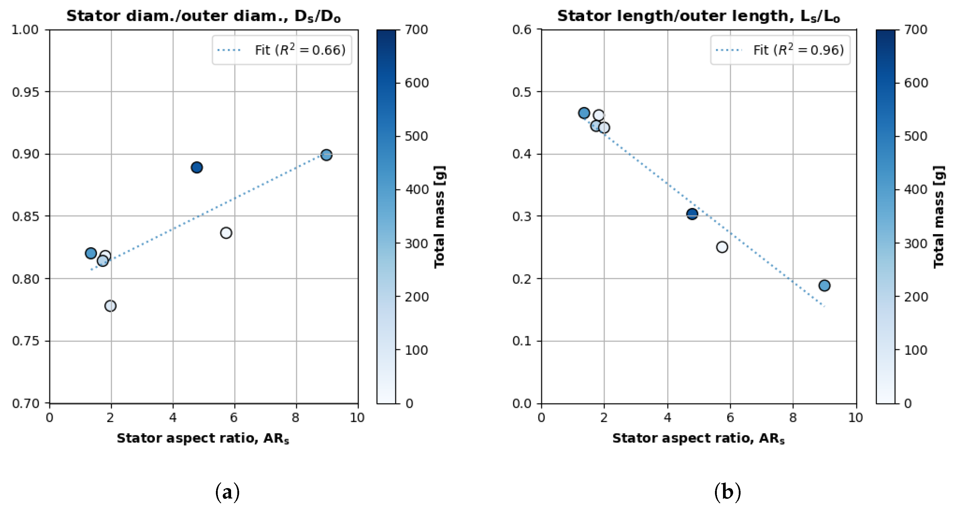
3.2. Geometry Trends
3.3. Figure-of-Merit Trends
4. Sizing Models and Validation
4.1. Mass
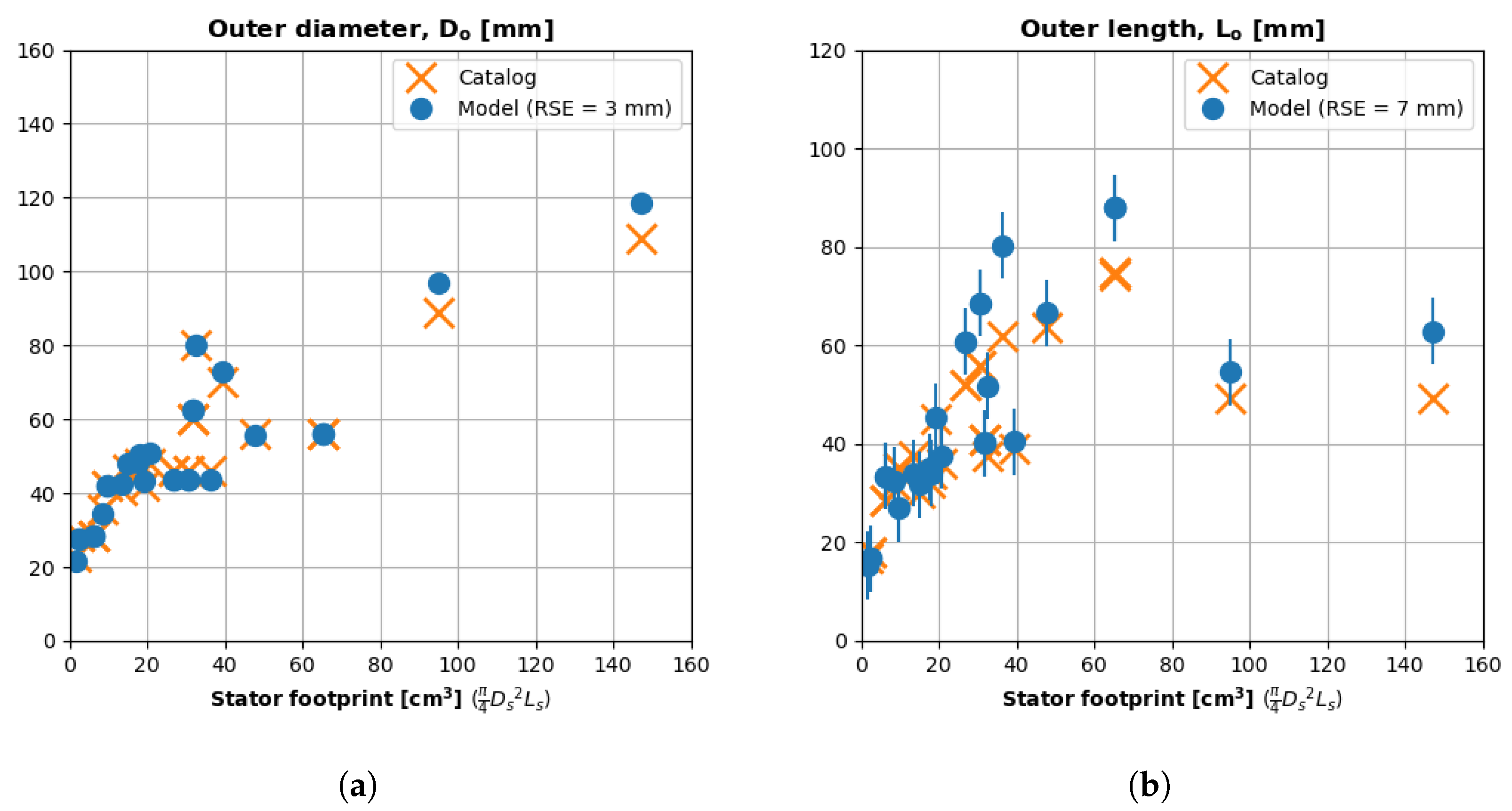
4.2. Geometry
4.3. Figure of Merit and Resistance
5. Full Sizing Algorithm
- Case 1.
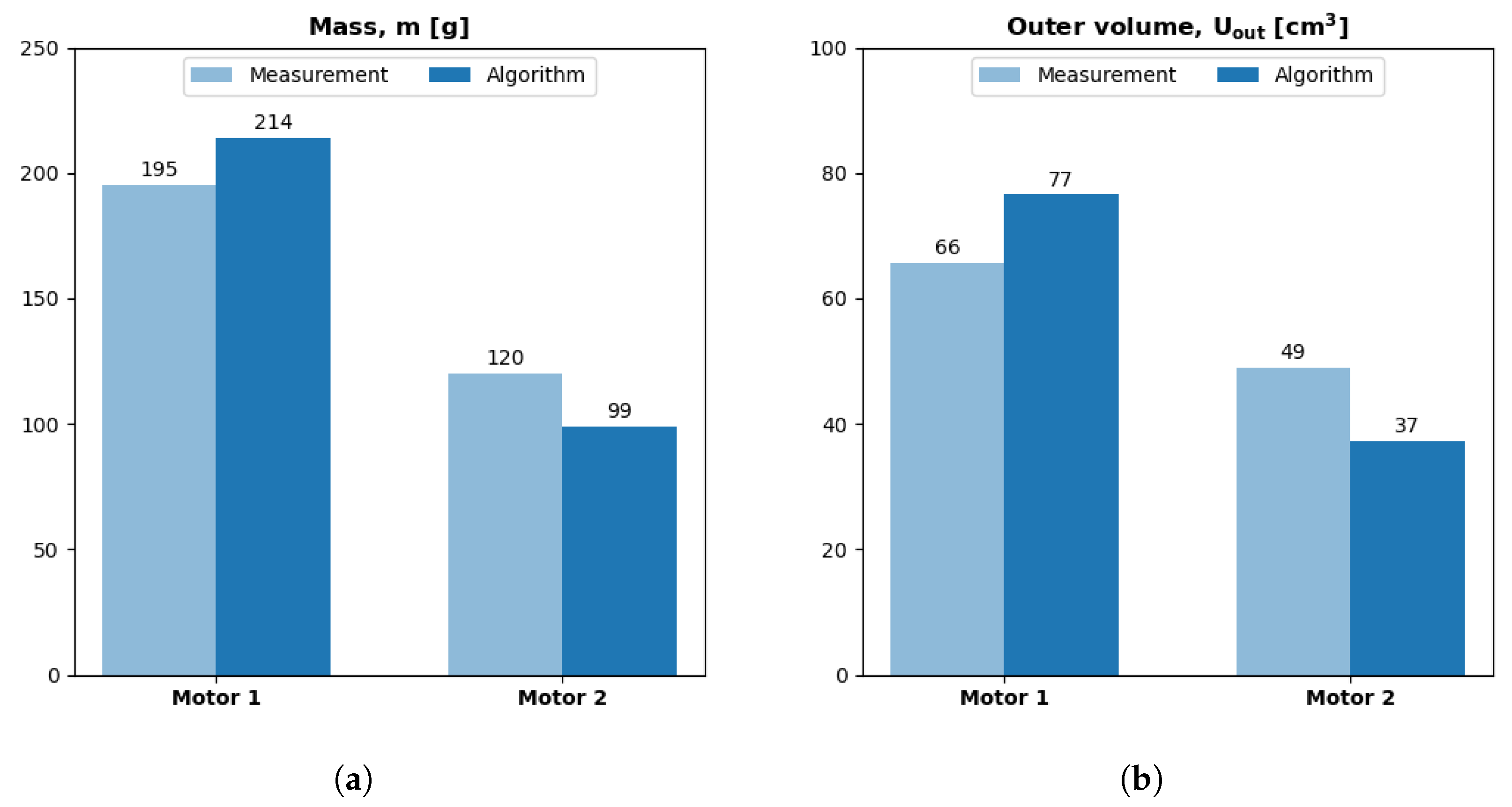
- Experimental validation: We compared the algorithm’s initial size, efficiency, and temperature predictions against experimental data for two different-sized motors under similar loads.
- Case 2.
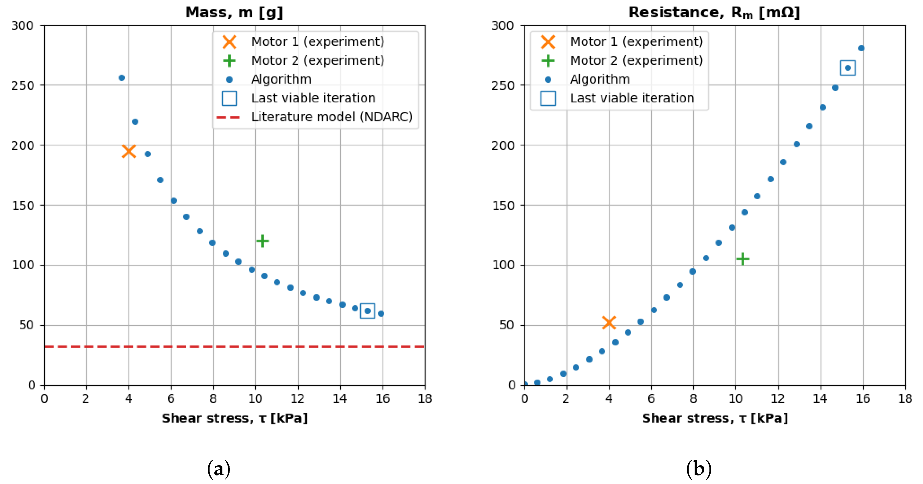
- Literature comparison: We compared the algorithm’s iterative predictions to literature models and experimental data.
- Case 3.
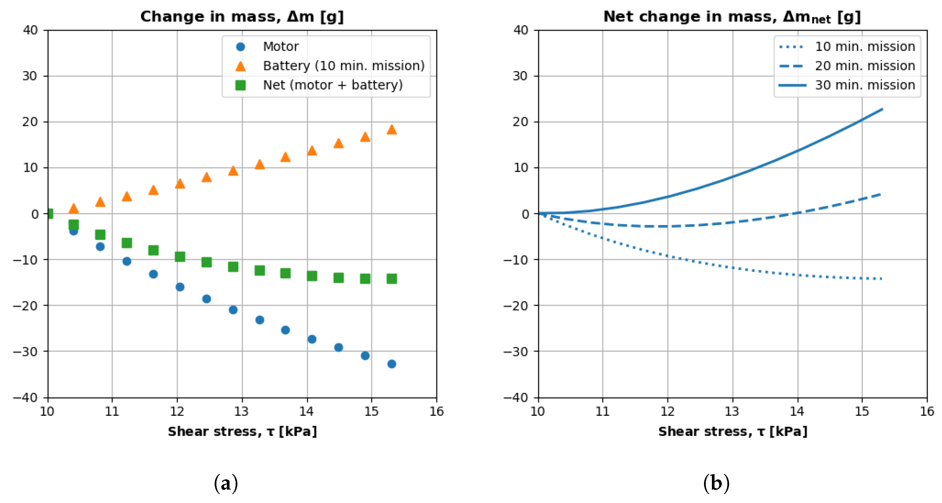
- Broader exploration: We coupled the motor algorithm with a reduced-order battery sizing model and examined the results from a mission-level perspective.
5.1. Experimental Validation
5.2. Literature Comparison
5.3. System-Level Integration
6. Discussion
6.1. Analysis
6.2. Future Work
7. Conclusions
Author Contributions
Funding
Data Availability Statement
Acknowledgments
Conflicts of Interest
Nomenclature
| A | Area [] |
| Stator aspect ratio [-] | |
| B | Motor magnetic loading [T] |
| Back-EMF margin [-] | |
| D | Diameter [m] |
| d | Throttle setting (duty-ratio) [-] |
| E | Energy [J] |
| e | Specific energy [J/kg] |
| h | Convective heat transfer coefficient [W/(K)] |
| I | Current [A] |
| Air thermal conductivity [W/(m·K)] | |
| Motor torque constant [N/(m·A)] | |
| L | Length [m] |
| M | Torque [N·m] |
| m | Mass [m] |
| Nusselt number [-] | |
| P | Power [W] |
| Reynolds number [-] | |
| Motor winding resistance [] | |
| T | Temperature [K] |
| t | Time [s] |
| U | Volume [] |
| u | Velocity [m/s] |
| DC voltage [V] | |
| w | Mass (weight) fraction [-] |
| Resistivity per unit length [m] | |
| Efficiency [-] | |
| Dynamic viscosity [/s] | |
| Density [kg/] | |
| Electromagnetic shear stress [Pa] | |
| Rotational speed [rad/s] |
References
- Johnson, W. NDARC-NASA Design and Analysis of Rotorcraft. In Proceedings of the American Helicopter Society Aeromechanics Specialists’ Conference, San Francisco, CA, USA, 20–22 January 2010; Available online: https://ntrs.nasa.gov/citations/20110002948 (accessed on 28 April 2024).
- Vegh, J.M.; Botero, E.; Clark, M.; Smart, J.; Alonso, J.J. Current capabilities and challenges of NDARC and SUAVE for eVTOL aircraft design and analysis. In Proceedings of the 2019 AIAA/IEEE Electric Aircraft Technologies Symposium (EATS), Indianapolis, IN, USA, 19–22 August 2019; IEEE: Piscataway, NJ, USA, 2019; pp. 1–19. [Google Scholar] [CrossRef]
- Sridharan, A.; Govindarajan, B.; Chopra, I. A scalability study of the multirotor biplane tailsitter using conceptual sizing. J. Am. Helicopter Soc. 2020, 65, 1–18. [Google Scholar] [CrossRef]
- Thurlbeck, A.P.; Cao, Y. Analysis and Modeling of UAV Power System Architectures. In Proceedings of the 2019 IEEE Transportation Electrification Conference and Expo (ITEC), Detroit, MI, USA, 19–21 June 2019; pp. 1–8. [Google Scholar] [CrossRef]
- Gong, A.; MacNeill, R.; Verstraete, D. Performance Testing and Modeling of a Brushless DC Motor, Electronic Speed Controller and Propeller for a Small UAV Application. In Proceedings of the 2018 Joint Propulsion Conference, Cincinnati, OH, USA, 9–11 July 2018. [Google Scholar] [CrossRef]
- Ma, Y.; Zhang, W.; Zhang, Y.; Ma, Y.; Bai, Z. Preliminary Design and Experimental Investigation of a Distributed Electric Propulsion Aircraft. In Proceedings of the 32nd Congress of the International Council of the Aeronautical Sciences (ICAS), Shanghai, China, 6–10 September 2021; pp. 6–10. [Google Scholar]
- Perry, A.T.; Ansell, P.J.; Kerho, M.F. Aero-propulsive and propulsor cross-coupling effects on a distributed propulsion system. J. Aircr. 2018, 55, 2414–2426. [Google Scholar] [CrossRef]
- Liang, D.; Zhu, Z.; Feng, J.; Guo, S.; Li, Y.; Wu, J.; Zhao, A. Influence of critical parameters in lumped-parameter thermal models for electrical machines. In Proceedings of the 2019 22nd International Conference on Electrical Machines and Systems (ICEMS), Harbin, China, 11–14 August 2019; IEEE: Piscataway, NJ, USA, 2019; pp. 1–6. [Google Scholar] [CrossRef]
- Tong, W. Mechanical Design and Manufacturing of Electric Motors; CRC Press: Boca Raton, FL, USA, 2022. [Google Scholar] [CrossRef]
- Mohan, N. Electric Machines and Drives, 1st ed.; Wiley: Hoboken, NJ, USA, 2012; Available online: https://books.google.com.hk/books?id=G-xHDwAAQBAJ&printsec=copyright&redir_esc=y#v=onepage&q&f=false (accessed on 1 June 2024).
- Hamdi, E.S. Design of Small Electrical Machines; John Wiley & Sons, Inc.: Hoboken, NJ, USA, 1994; Available online: https://dl.acm.org/doi/abs/10.5555/561305 (accessed on 28 April 2024).
- Hendershot, J.; Miller, T. Design of Brushless Permanent-Magnet Machines; Oxford Academic: Oxford, UK, 2010. [Google Scholar] [CrossRef]
- Kirchgässner, W.; Wallscheid, O.; Böcker, J. Estimating electric motor temperatures with deep residual machine learning. IEEE Trans. Power Electron. 2020, 36, 7480–7488. [Google Scholar] [CrossRef]
- Ugwueze, O.; Statheros, T.; Horri, N.; Bromfield, M.A.; Simo, J. An Efficient and Robust Sizing Method for eVTOL Aircraft Configurations in Conceptual Design. Aerospace 2023, 10, 311. [Google Scholar] [CrossRef]
- Miyairi, Y.; Perullo, C.; Mavris, D.N. A parametric environment for weight and sizing prediction of motor/generator for hybrid electric propulsion. In Proceedings of the 51st AIAA/SAE/ASEE Joint Propulsion Conference, Orlando, FL, USA, 27–29 July 2015; p. 3887. [Google Scholar] [CrossRef]
- Tursini, M.; Villani, M.; Fabri, G.; Di Leonardo, L. A switched-reluctance motor for aerospace application: Design, analysis and results. Electr. Power Syst. Res. 2017, 142, 74–83. [Google Scholar] [CrossRef]
- Dussart, G.X.; Lone, M.M.; O’Rourke, C. Size estimation tools for conventional actuator system prototyping in aerospace. In Proceedings of the AIAA Scitech 2019 Forum, San Diego, CA, USA, 7–11 January 2019; p. 1634. [Google Scholar] [CrossRef]
- Roussel, J.; Budinger, M.; Ruet, L. Preliminary Sizing of the Electrical Motor and Housing of Electromechanical Actuators Applied on the Primary Flight Control System of Unmanned Helicopters. Aerospace 2022, 9, 473. [Google Scholar] [CrossRef]
- Saemi, F.; Whitson, A.; Benedict, M. Heat Transfer Models and Measurements of Brushless DC Motors for Small UASs. Aerospace 2024, 11, 401. [Google Scholar] [CrossRef]
- Koegler, L. KDE4215XF-465 Brushless DC Motor; KDE Direct, LLC: Bend, OR, USA, 2024; Available online: https://www.kdedirect.com/blogs/news/18013663-4215xf-465-uas-brushless-motor (accessed on 28 April 2024).
- Burress, T.A.; Campbell, S.L.; Coomer, C.; Ayers, C.W.; Wereszczak, A.A.; Cunningham, J.P.; Marlino, L.D.; Seiber, L.E.; Lin, H.T. Evaluation of the 2010 Toyota Prius Hybrid Synergy Drive System; Technical report; Oak Ridge National Lab. (ORNL): Oak Ridge, TN, USA, 2011. [Google Scholar] [CrossRef]
- Staunton, R.H.; Burress, T.A.; Marlino, L.D. Evaluation of 2005 Honda Accord Hybrid Electric Drive System; Technical report; Oak Ridge National Lab. (ORNL): Oak Ridge, TN, USA, 2006. [Google Scholar] [CrossRef]
- Saemi, F.; Benedict, M. Flight-Validated Electric Powertrain Efficiency Models for Small UASs. Aerospace 2023, 11, 16. [Google Scholar] [CrossRef]
- Hanselman, D. Brushless Permanent Magnet Motor Design. The Writers’ Collective. 2003. Available online: https://digitalcommons.library.umaine.edu/fac_monographs/231 (accessed on 24 June 2024).
- Bolam, R.C.; Vagapov, Y.; Anuchin, A. Performance Comparison between Copper and Aluminium Windings in a Rim Driven Fan for a Small Unmanned Aircraft Application. In Proceedings of the 2020 XI International Conference on Electrical Power Drive Systems (ICEPDS), St. Petersburg, Russia, 4–7 October 2020; pp. 1–6. [Google Scholar] [CrossRef]
- Hughes, A.; Drury, W. Electric Motors and Drives: Fundamentals, Types and Applications; Newnes: Oxford, UK, 2013. [Google Scholar] [CrossRef]
- Koegler, L. KDE 10218XF-105 Brushless DC Motor; KDE Direct, LLC: Bend, OR, USA, 2024; Available online: https://www.kdedirect.com/products/kde10218xf-105 (accessed on 24 June 2024).
- Koegler, L. KDE 4014XF-380 Brushless DC Motor; KDE Direct, LLC: Bend, OR, USA, 2024; Available online: https://www.kdedirect.com/products/kde4014xf-380 (accessed on 24 June 2024).
- Koegler, L. KDE3510XF-475 Brushless DC Motor; KDE Direct, LLC: Bend, OR, USA, 2024; Available online: https://www.kdedirect.com/products/kde3510xf-475 (accessed on 24 June 2024).
- Toliyat, H.A.; Kliman, G.B. Handbook of Electric Motors; CRC Press: Boca Raton, FL, USA, 2018. [Google Scholar] [CrossRef]
- Coleman, D.; Halder, A.; Saemi, F.; Runco, C.; Denton, H.; Lee, B.; Subramanian, V.; Greenwood, E.; Lakshminaryan, V.; Benedict, M. Development of “Aria” a Compact, Quiet Personal Electric Helicopter. J. Am. Helicopter Soc. 2023, 68, 42011–42024. [Google Scholar] [CrossRef]
- Bird, J.Z. A Review of Electric Aircraft Drivetrain Motor Technology. IEEE Trans. Magn. 2022, 58, 1–8. [Google Scholar] [CrossRef]


| Motor | 1 | 2 | 3 | 4 | 5 | 6 | 7 | |
|---|---|---|---|---|---|---|---|---|
| Mass, m | [g] | 24 | 49 | 97 | 208 | 379 | 412 | 598 |
| Stator aspect ratio, | [-] | 5.8 | 1.8 | 2.0 | 1.8 | 9.0 | 1.4 | 4.8 |
| Stator inner diameter, | [mm] | 10.0 | 9.5 | 12.7 | 12.9 | 29.7 | 13.9 | 29.9 |
| Stator diameter, | [mm] | 23.0 | 22.0 | 28.0 | 35.0 | 72.0 | 41.0 | 72.0 |
| Rotor inner diameter, | [mm] | 21.2 | 22.9 | 29.0 | 36.0 | 73.0 | 41.6 | 73.2 |
| Motor outer diameter, | [mm] | 27.5 | 26.9 | 36.0 | 43.0 | 80.1 | 50.0 | 81.0 |
| Stator length, | [mm] | 4.0 | 12.0 | 14.0 | 20.0 | 8.0 | 30.0 | 15.0 |
| Motor outer length, | [mm] | 16.0 | 26.0 | 31.7 | 45.0 | 42.5 | 64.5 | 49.5 |
| Motor | 1 | 2 | 3 | 4 | 5 | 6 | 7 |
|---|---|---|---|---|---|---|---|
| Stator | 0.32 | 0.41 | 0.39 | 0.50 | 0.45 | 0.50 | 0.50 |
| Rotor | 0.28 | 0.31 | 0.36 | 0.25 | 0.16 | 0.28 | 0.19 |
| Stator support | 0.12 | 0.09 | 0.10 | 0.04 | 0.13 | 0.01 | 0.04 |
| Rotor support | 0.12 | 0.12 | 0.07 | 0.10 | 0.14 | 0.14 | 0.15 |
| Bearings | 0.11 | 0.03 | 0.05 | 0.05 | 0.07 | 0.02 | 0.08 |
| Shaft | 0.05 | 0.03 | 0.04 | 0.05 | 0.06 | 0.04 | 0.05 |
| Motor 1 | Motor 2 | Mean | |||
|---|---|---|---|---|---|
| Mass | m | 195 | 120 | 158 | g |
| Applied torque | M | 167 | 199 | 183 | N·mm |
| Applied rotational speed | 3965 | 4700 | 4333 | min | |
| Freestream velocity | 9.8 | 10.3 | 10.1 | m/s | |
| Freestream temperature | 24.0 | 24.0 | 24.0 | °C | |
| Shear stress | 4.0 | 10.3 | 7.2 | kPa | |
| Stator aspect ratio | 2.8 | 3.5 | 3.2 | ||
| DC voltage | 12.0 | 13.0 | 12.5 | V | |
| No-load current | 0.2 | 0.7 | 0.5 | A | |
| Full motor specifications | Ref. [20] | Ref. [29] |
Disclaimer/Publisher’s Note: The statements, opinions and data contained in all publications are solely those of the individual author(s) and contributor(s) and not of MDPI and/or the editor(s). MDPI and/or the editor(s) disclaim responsibility for any injury to people or property resulting from any ideas, methods, instructions or products referred to in the content. |
© 2024 by the authors. Licensee MDPI, Basel, Switzerland. This article is an open access article distributed under the terms and conditions of the Creative Commons Attribution (CC BY) license (https://creativecommons.org/licenses/by/4.0/).
Share and Cite
Saemi, F.; Benedict, M. Brushless DC Motor Sizing Algorithm for Small UAS Conceptual Designers. Aerospace 2024, 11, 649. https://doi.org/10.3390/aerospace11080649
Saemi F, Benedict M. Brushless DC Motor Sizing Algorithm for Small UAS Conceptual Designers. Aerospace. 2024; 11(8):649. https://doi.org/10.3390/aerospace11080649
Chicago/Turabian StyleSaemi, Farid, and Moble Benedict. 2024. "Brushless DC Motor Sizing Algorithm for Small UAS Conceptual Designers" Aerospace 11, no. 8: 649. https://doi.org/10.3390/aerospace11080649