Abstract
Recently, the world’s first plasma-propelled drone was successfully flown, demonstrating that plasma propulsion technology is suitable for drone flight. The research on plasma propulsion drones has sparked a surge of interest. This study utilized a proxy model and the NSGA-II multi-objective genetic algorithm to optimize the geometric parameters based on staggered thrusters that affect the performance of electroaerodynamics (EAD) thrusters used for solid-state plasma aircraft. This can help address key issues, such as the thrust density and the thrust-to-power ratio of solid-state plasma aircraft, promoting the widespread application of plasma propulsion drones. An appropriate sample set was established using Latin hypercube sampling, and the thrust and current data were collected using a customized experimental setup. The proxy model employed a genetically optimized Bayesian regularization backpropagation neural network, which was trained to predict the effects of variations in the geometric parameters of the electrode assembly on the performance parameters of the plasma aircraft. Based on this information, the maximum achievable value for a given performance parameter and its corresponding geometric parameters were determined, showing a significant increase compared to the sample data. Finally, the optimal parameter combination was determined by using the NSGA-II multi-objective genetic algorithm and the Analytic Hierarchy Process. These findings can serve as a basis for future researchers in the design of EAD thrusters, helping them produce plasma propulsion drones that better meet specific requirements.
1. Introduction
Since the Wright Brothers achieved the first controlled human flight over a hundred years ago, aircraft within the atmosphere have been propelled by propellers and gas turbine engines, mostly powered by fossil fuels. The current trend is to replace chemical fuel propulsion systems with electric propulsion systems to reduce carbon emissions. In the aerospace field, electric propulsion technology is considered an alternative to fossil fuel technology [1]. Ion thrusters have been widely and successfully used in space applications [2]. In recent years, there has been a growing interest in Electrohydrodynamic (EHD) propulsion in this field, with initial applications in atmospheric flight. Ion propulsion, as an alternative to traditional engines, offers many advantages, such as no moving parts, a high thrust-to-power ratio, low noise, and high sustainability of the propulsion system [3].
In 1928, Brown constructed a pair of asymmetric electrodes that generated directional propulsion in the air using high voltages (i.e., tens of kilovolts) [4]. Two electrode rods with different radii of curvature constituted the propulsion structure; the emitter electrode had the lower radius of curvature, and the collector electrode rod had the larger radius of curvature. The asymmetric electrode structure produces thrust based on the principle that a high-voltage electric field generates ions via the ionization of neutral air molecules, and the field also accelerates the ions. Because of the isotropic motion, the accelerated ions collide with neutral molecules, exchanging momentum with them to drive the ions forward [5]. The study of these dynamics is known as electroaerodynamics (EAD). EAD has been studied and utilized in the areas of gas pumping [6,7], flow control [8,9], and air purification [10,11].
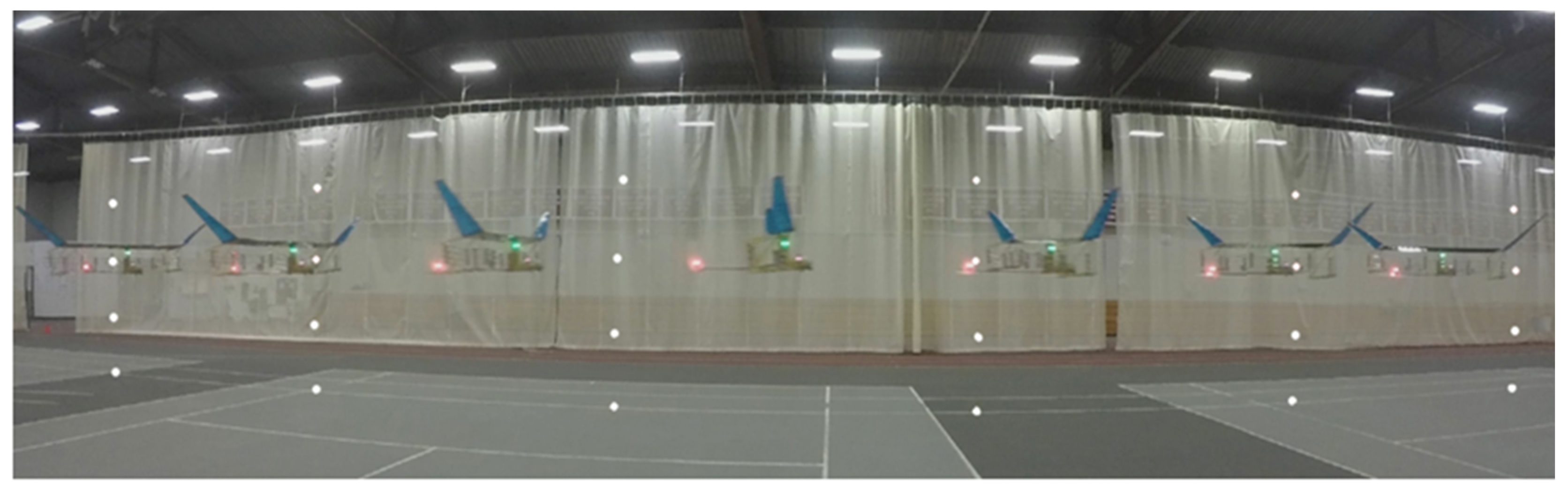
Because EAD devices do not have moving elements, such as turbines and propellers, they have progressively garnered more interest; in fact, they may be able to replace other propellers used in aircraft propulsion. In 2009, researchers from NASA analyzed and demonstrated the use of plasma propulsion technology (EAD propulsion) for unmanned aerial vehicles (UAVs). They concluded that because of the technology’s low thrust, it was unlikely to be used as the primary thrust generator in UAVs [12]. Pekker and Young [13] concluded that the thrust density of plasma propulsion was insufficient for aircraft propulsion. However, research on plasma propulsion technology is still ongoing, and a number of researchers have pioneered the use of plasma propulsion in hot-air balloons and airships. For example, in 2014, Johnson et al. [14] proposed a pulsed EAD thruster design for high-altitude, long-endurance airships. Similarly, in 2016, Wynsberghe et al. [15] suggested using an EAD thruster to drive a stratospheric hot-air balloon. In 2017, Khomich and Rebrov [16] incorporated a transmitter and receiver into a wireless power transmission device for use in an EAD thruster designed for vertical takeoffs. In 2018, Drew and Lambert [17] developed and successfully launched a small (2 cm × 2 cm) and lightweight (30 mg) microrobot with a thrust-to-weight ratio of 10. Also in 2018, researchers [2] from the Massachusetts Institute of Technology successfully tested the world’s first plasma-propelled drone (as shown in Figure 1), demonstrating that plasma propulsion technology is suitable for drone flight. In 2019, Chirita and Ieta [5] completed their first unmanned flight with a rotary ion engine (RIE), which used ionized wind to blow the rotor blades.

Figure 1.
Time-lapse image of the EAD aircraft in flight.
The fixed-wing plasma aircraft flown by the Massachusetts Institute of Technology, which featured a high-voltage power converter and an EAD thruster, is shown in Figure 2. Compared with traditional aviation propellers (piston and jet engines), plasma propulsion vehicles exhibit low fatigue, are ultra-quiet, and have long service lives owing to their simple structure and lack of moving parts. In addition, electrical propulsion does not contaminate the environment. Compared to the typical thrust-to-power ratio of conventional aerospace propulsion technology (3 N/kW), the predicted thrust-to-power ratio of the EAD aircraft (50 N/kW) was substantially higher in the laboratory [18]. However, the low propulsion and thrust density of EAD thrusters have constrained their application in small UAVs. Accordingly, in recent years, many researchers have worked on designing lightweight and high-voltage power converters (HVPCs) [19,20,21] that will improve thruster propulsion performance.
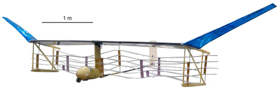
Figure 2.
Photograph of the actual EAD aircraft tested by MIT, including its high-voltage power converter and EAD thruster.
The fundamental component of an EAD thruster, also called a thruster unit, is an asymmetric pair of electrode rods. One electrode is called the emitter and the other is called the collector; they are separated by an electrode gap d and connected to a high-voltage source. The collector typically has a larger frontal area, such as that of a cylinder or airfoil, and the emitter typically has a very small radius of curvature. In early studies, such as those carried out by Moreau and Benard [22], the effects of the electrode gap d, air humidity, and cylinder diameter of the grounded electrodes on the thruster were investigated. Subsequent experiments with EAD thrusters have shown that the thrust-to-power ratio and thrust density of EAD thrusters in small unmanned aircraft can be increased by using series and parallel arrangements [23,24]. In this context, a series connection refers to a plurality of thruster units connected head to tail and placed in the same plane, which form a multistage thruster. A parallel connection refers to a plurality of thrusters, with emitters in one plane and collectors in the other; the two planes are parallel. Examples of thruster unit geometries include wire to cylinder [25], wire to airfoil [17], and pin to mesh [16]. Early research primarily focused on the wire-to-cylinder geometry, but switching to an airfoil significantly minimizes the drag caused by the plasma flow. This finding was confirmed by Belan et al. [26], who also investigated the effect of using collectors with different airfoil shapes on the propulsion performance. Their findings demonstrated the necessity for further systematic studies on electrode geometries. In addition, Belan et al. [27] tested the effect of emitter density on the plasma thruster performance and determined that an optimal collector–emitter spacing ratio exists.
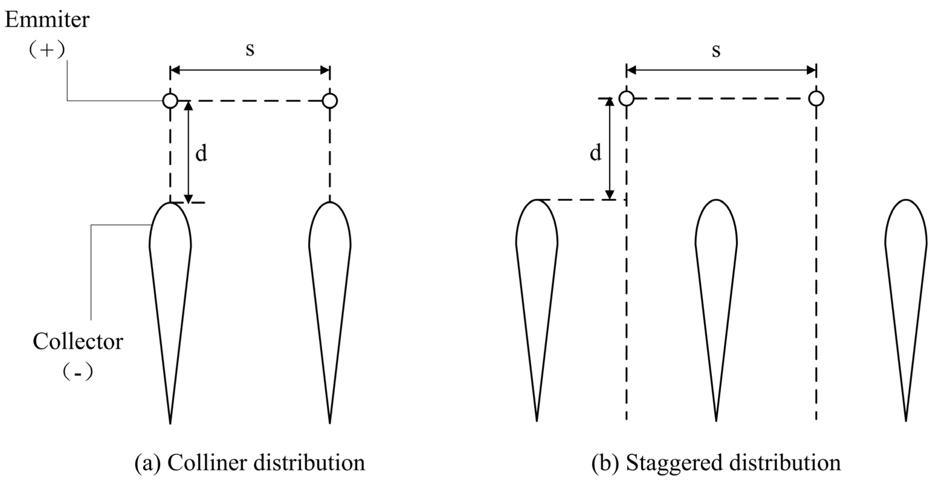
In previous performance optimization experiments, two primary electrode distribution patterns were examined for their effects on the electrical parameters (e.g., voltage and polarity) and geometrical parameters (e.g., the thruster unit spacing s between two parallel emitters or collectors and the electrode gap d between the emitters and the collectors). As shown in Figure 3, when the emitter is located above the collector, it is called the collinear distribution, which is used in the majority of studies [18]. When the emitter is placed in the middle of succeeding collectors, it is called the staggered distribution, which operates according to the same physical principles [17]. Moreau’s experimental data indicated that the current-to-thrust conversion is more efficient for the staggered electrode distribution [3]. This phenomenon was confirmed in Monrolin’s study [25]; however, he did not further theorize about its cause.

Figure 3.
Two main electrode distribution types.
The effects of a single-variable thruster unit geometry and the coupling of two to three variables on the propulsion performance have been well-studied. However, when the collectors are airfoils, the plasma thruster design requires accounting for additional variables and is characterized by nonlinearity and principal unknowns. As mentioned above, researchers have not yet conducted a comprehensive and detailed investigation into the impact of the geometric configuration of the thruster on the performance of the plasma thruster due to the various challenges involved in conducting physical experiments on plasma thrusters, which is what we are considering implementing. To simplify the thruster design, a proxy model is required. A proxy model is a mathematical or statistical model used to represent, simulate, or predict a system, phenomenon, or process. It is typically a simplification or approximation of a real system that captures its key factors and interactions for simulation purposes. It can contribute to understanding problems, making predictions, and optimizing decisions [28].
The main purpose of this article is to conduct a detailed study of the five most significant parameters that affect the performance of plasma thrusters, aiming to achieve performance optimization. This is beneficial for improving the thrust density and thrust-to-power ratio issues currently faced by plasma thruster drones, thereby enhancing their utility. A thruster unit configuration consisting of a staggered distribution of emitters and collectors was tested because it produces less parasitic drag and yields superior aerodynamic effects. We aimed to select a reasonable sampling method to collect the sample points and establish an approximate proxy-based model, thereby ensuring that the output response values of the model would achieve the desired accuracy. Finally, we aimed to optimize the performance of the thruster unit through a multi-objective genetic algorithm.
The remainder of this paper is organized as follows. Section 2 briefly elaborates on the one-dimensional EAD theory, explaining why electrodes in a staggered distribution can decrease drag and provide a useful parametric design space. Section 3 introduces the customized experimental setup. Section 4 explains the optimization design method, including the sampling method, proxy model, and multi-objective genetic algorithm. Section 5 presents the predicted results of the proxy model and the optimized parameters, followed by a comparison and validation. Finally, Section 6 contains the conclusions of the study.
2. Theory
2.1. Basic Theoretical Analysis
Hydrodynamics and electrodynamics were combined in a one-dimensional EAD thrust model to provide theoretical guidance for thruster performance evaluation and to consolidate the primary factors involved in thrust. The corona discharge region resulting from EAD propulsion can be divided into the ionization and ion drift zones. The ionization zone close to the emitter is influenced by a high-voltage electric field, which ionizes the surrounding gas. However, beyond a certain distance, the electric field’s strength is insufficient to maintain the ionization, and the ions move into the drift zone. Under the influence of the electric field, the ions in the drift region continue to travel toward the collectors as they collide with neutral gas molecules, transferring momentum and kinetic energy in the process. In the drift region, the ions only contribute to the charge density ρ. The ion velocity vi is composed of two separate velocity terms: the air velocity u and the ion mobility velocity μE. The μ is the ion mobility (which depends on the temperature and the pressure) and E is the electric field’s strength. Therefore, the ion velocity is given by
Assuming that the system is stable and that no time-varying electric or magnetic field is present, a current is produced by the movement of charges between the emitter and the collector electrodes; the current density j can be expressed as
The volume force is equal to the electrostatic Coulomb force exerted on the ions by the electrodes [25]. Therefore, in the discharge volume, the EAD thrust acting on the charged particles per unit volume is defined as
Consequently, the EAD thrust delivered to the discharge volume is
and the discharge current flowing through the unit area is
Previous experiments have concluded that, in most cases, the average electric field strength is Vm−1 and the ion mobility is m2V−1s−1, which results in an ion migration velocity estimation of at least 100 m/s; this value is much larger than the velocity of the air flow (μ). Thus, Equation (5) can be simplified to
where A is the cross-sectional area of the corona discharge electrode. Combining Equations (2) and (4), we obtain
where d is the electrode gap between the emitters and collectors and x is a one-dimensional coordinate between the electrodes. The coordinate of the emitter’s location is x = 0, and the coordinate of the collector’s location is x = d.
Because the corona discharge ionizes the air surrounding the EAD thruster, both the ion species and ion mobility are constant. Thus, the space charge limits the corona discharge, causing the electric field strength and charge density to constrain each other. Additionally, the relationship between the voltage and the current can be captured according to the empirical law of corona discharge [29], which is expressed as
where C is an empirical constant that depends on the electrode geometry and ion mobility μ, Va is the working voltage applied to the electrode, and V0 is the corona onset voltage. Combined with Equation (8), the EAD thrust can be expressed as
The constant C in Equation (9) is expressed as
where is the dielectric constant of the air, l is the length of the electrode, and is a dimensionless constant. Thus,
Equation (11) indicates that in the one-dimensional EAD thrust model, the thrust is inversely proportional to the electrode gap for a constant working voltage. Furthermore, the thrust-to-power ratio is
where P denotes the power, which is the product of the thruster’s current and the working voltage. In the absence of resistance, the thrust per unit volume of the electrode is
where V is the thruster’s working volume.
2.2. Staggered Distribution Resistance
In addition to thrust, aerodynamic drag must be considered. The aerodynamic drag usually acts on the collectors and has a negligible effect on the emitters. The difference between the EAD thrust and drag D is known as the effective thrust , and it is expressed as
The staggered electrode distribution aerodynamically outperforms the collinear electrode distribution in terms of effective thrust, primarily because of the drag force D.
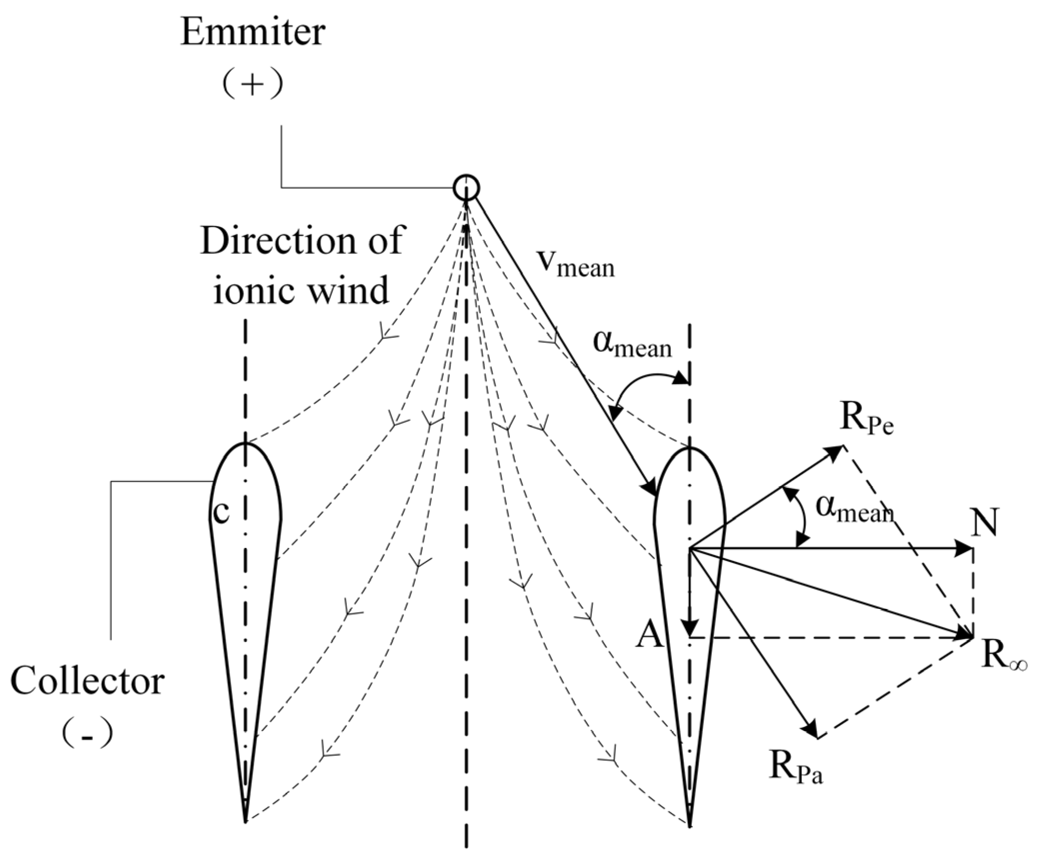
The line connecting the leading and trailing edges of an airfoil is called the chord, and its length is denoted as c. For a staggered electrode distribution, the emitter is located halfway between the two collectors. Ions in the ionization zone move toward the collectors on either side of the drift zone, resulting in an ionic vi that does not coincide with the chord. Thus, the mean wind deflection angle, represented by αmean, is defined as the angle between the mean ionic velocity and the chord in the plane of the airfoil. As shown in Figure 4, the wind deflection angle of the chord is positive when the incoming ionized wind speed is deflected to the left and negative when it is deflected to the right. To determine the magnitude of the drag for different distributions, we examined the aerodynamic forces acting on the unit spread length of the airfoil. A pressure p and a shear stress τ act on each point of the airfoil’s surface. These pressure and shear stress distributions combine to form an arbitrary planar force system, the total force of which is . The intersection between the direction of and the chord must be determined. The total aerodynamic force can be decomposed into two components: one perpendicular to the mean ionic velocity, , and one parallel to the mean ionic velocity, . It is also possible to decompose into two other components: one perpendicular to the direction of the chord (denoted as the normal force N) and one parallel to the direction of the chord (denoted as the axial force A). The four variables just mentioned can be summarized as follows:
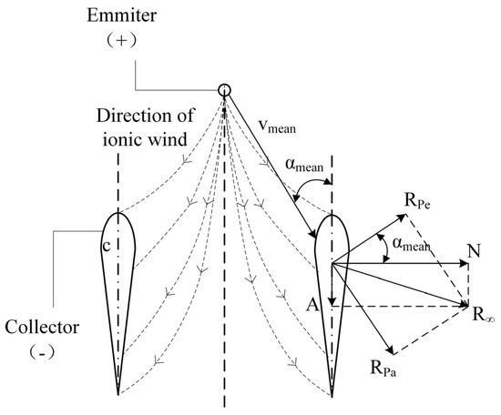
Figure 4.
Direction of ionized wind and the aerodynamic components in the staggered distribution of thruster units.
For the two-dimensional winding problem, the drag coefficient cd of the airfoil and the dynamic pressure were utilized to represent the drag D associated with the collectors, according to
where is the air density and is the pressure of the flow generated by the ionized wind. The ion wind speed u is a function of the working voltage and the electrode gap d, the values of which are independent of the electrode distribution. Similarly, the two components of the total aerodynamic force are expressed as
where and are the aerodynamic coefficients corresponding to the directions perpendicular and parallel to the incoming ionized wind, respectively.
For a collinear distribution, the ionized wind speed is approximately parallel to the direction of the chord, and hence the mean wind speed deflection angle is 0:
The mean air flow deflection remains zero, even when accounting for the mutual influence of nearby electrode pairs. The normal forces operating on each individual collector electrode airfoil cancel each other. Thus, the airfoil drag is equal to the axial force, as expressed by
where the subscript “Co” denotes the collinear distribution.
Figure 4 shows an analysis of the aerodynamic effects of the individual emitters and collectors in the staggered electrode distribution; the drag exerted on this distribution is represented by
To simplify the analysis, it was assumed that a single collector receives ions only from the neighboring emitters. The airfoil is subjected to aerodynamic forces in both directions; when the normal force on the airfoil is 0, the term in the axial force equation is 0, and the expression for the airfoil drag becomes
These equations indicate that one of the main reasons the drag exerted on the staggered distribution is smaller than that exerted on the collinear distribution is the deflection angle of the ionized air flow caused by the staggered distribution design.
2.3. Space and Analysis of Performance Parameters
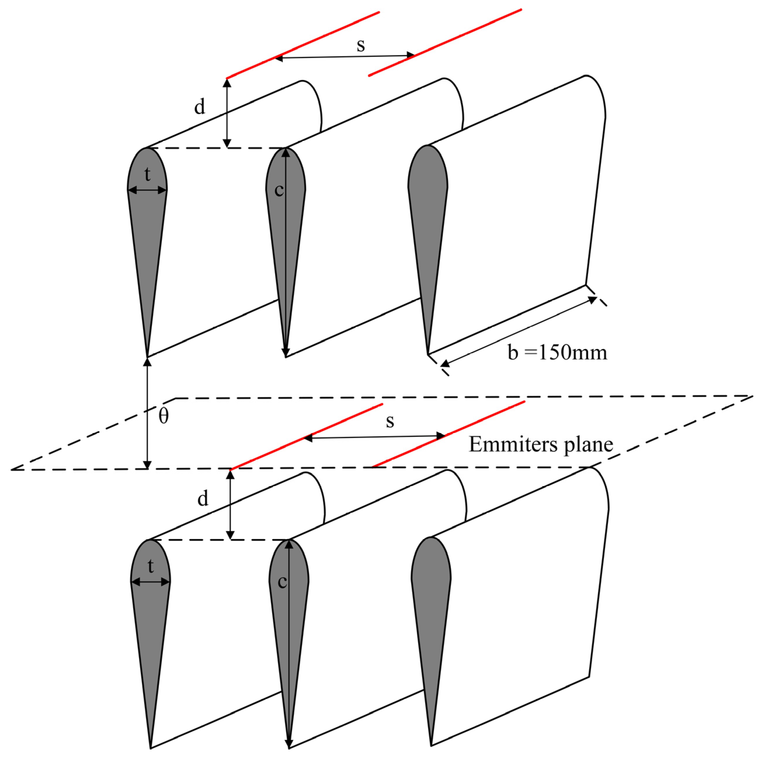
The parameters considered in the evaluation of the EAD thruster were the electrode distribution, the electrode gap d, the thruster unit spacing s, the multistage thruster stage spacing θ, and the geometric configuration of the collector. After deciding on a staggered distribution for the electrodes and an airfoil geometry for the collector, the thickness and chord length of the airfoil were determined as its primary geometric parameters, corresponding to the 4-digit NACA airfoil. Therefore, a total of five design parameters required experimental testing: d, s, θ, c, and the maximum airfoil thickness t. A description of the parameter space definition is shown in Figure 5. According to the experimental findings of earlier studies, defining the range of these five parameters is sufficient to guarantee that the ideal performance index falls within this range. The selection ranges for each parameter are listed in Table 1.
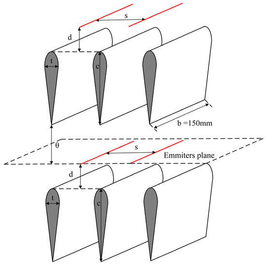
Figure 5.
Performance space of the selected parameters.

Table 1.
Multistage EAD thruster design variables and their ranges.
The effect of parameter d on the thruster performance was analyzed through a basic theoretical analysis. Gilmore and Barrett experimentally determined the relationship between the total thrust and the s/d ratio of two collinear wire-to-cylinder electrode sets connected in parallel, which was adequately expressed by an exponential function. In addition, thin airfoils with excessively long chords perform poorly. This is because the friction caused by excessively long walls introduces a significant amount of parasitic drag, resulting in a substantial reduction in the effective thrust for collector electrodes with airfoil geometry. Furthermore, reducing the chord length for a constant thickness results in a similar discharge cross-section for the corona discharge, thereby preserving a similar electric thrust. As the aspect ratio increases, the airfoil’s leading edge gradually becomes blunter, resulting in a degraded aerodynamic performance. This phenomenon can also occur if the thickness is increased while the chord length remains constant. Moreover, an excessively small θ can lead to a reverse-discharge phenomenon, generating a reverse-ion wind.
3. Optimization of the Design Methods
3.1. Experimental Design
The optimal design process for the target parameters in this study was divided into three steps: experimental design, proxy model building, and genetic algorithm optimization. The experimental design employed Latin hypercube sampling (LHS), which has the significant advantage of being able to construct a high-precision analytical model that is very similar to the actual model but with a smaller number of experimental samples, thereby substantially reducing the computational load. This method can be used to select the sample points more evenly within a sampling range. The choice of sampling strategy has a certain impact on the performance and generalization ability of the model, but if the ranges of parameter values are too large or too many samples are collected, the efficiency of the experiment will decrease and the experiment will be prolonged. However, too few samples may cause the proxy model to overfit or underfit, increase the instability during the sample training process, and reduce the generalization ability.
LHS is an equal-probability stratified sampling method that randomly generates samples within a range of values for each parameter [30,31]. For this study, LHS indicated that the sample size should be more than three times that of the number of design parameters. There were five design parameters for the thruster; therefore, a minimum of 15 tests should be performed. However, we chose to perform three times this number of tests to obtain more accurate results. Thus, 45 samples were collected. According to the sampling principle, the independent space of each parameter was evenly divided into 45 parts, and then a parameter point was randomly selected in each part of the independent space. A random combination of five sets of design parameters yielded 45 sample points. When a comparatively limited number of samples was used for probing, these 45 sample points performed better because they were highly homogenized, covered all regions of the parameter space, and were well-covered. Table A1 lists the 45 sample points selected for this study.
3.2. Proxy Model Building
Proxy models based on artificial neural networks are frequently used to establish relationships between inputs and outputs [32]. Neural networks attempt to (at least partially) simulate the structure and function of the brain and nervous system in living organisms [33,34]. Accordingly, they consist of interconnected neurons that can simulate the signal transmission that occurs between neurons in the human brain, thereby automating the learning and decision-making process. Thus far, the error backpropagation algorithm combines several optimization algorithms, such as gradient descent, to continuously adjust weights and biases based on training data, thereby enhancing the model’s accuracy and generalization capability [33]. Therefore, it is considered one of the most successful learning algorithms for feedforward neural networks. BP neural networks consist of a forward propagation process for the working signal and a backward propagation process for the error signal. BP neural networks process m inputs and produce n outputs, and they typically consist of three layers: input, hidden, and output. However, several hidden layers can be placed between the input and output layers. A three-layer BP network is capable of mapping from m-dimensions to n-dimensions. The numbers of neurons in the input and output layers are fixed. The number of neurons in the hidden layer can be determined according to the empirical formula
where q, m, and n are the numbers of neurons in the hidden, input, and output layers, respectively, and a is a conditioning constant between 1 and 10. In this study, the input layer defined five input neurons (d, s, t, c, and θ), and the output layer defined two output neurons (Te and P). Based on Equation (22), the preliminary determination of the number of neurons in the hidden layer was between 4 and 13. The best structure was determined via trial and error. Testing the performance of the neural network in each of these cases revealed that the performance parameters of the plasma thruster can be effectively predicted using six hidden-layer neurons.
The dataset, consisting of 45 sample points, was divided into three sets: training, validation, and test. The training, validation, and test sets contained 31, 7, and 7 sample points, respectively. To speed up the training process, we used the purelin linear transfer function and the Levenberg–Marquardt algorithm as training methods for the neural network. Compared to traditional gradient descent algorithms, the approach typically converges more quickly to local optimal solutions. It is beneficial for both the training speed and performance of neural networks, while mitigating issues, such as gradient vanishing and exploding. The dataset was normalized to linearly scale the input values within the range (0, 1]. The network training error was the average relative error between the predicted and actual values of the sample points.
Because the selection of the neural network structure, initial connection weights, and thresholds has a significant impact on network training but is difficult to obtain accurately, we used a genetic algorithm coupled with a neural network to initialize the initial weights and thresholds and perform the optimization. The basic idea was to use an individual to represent the initial weights and thresholds of the network, calculate the average relative error between the predicted and actual values of the test set as the output of the objective function, and then calculate the fitness value of the individual. Through the selection, crossover, and mutation operations, we searched for the individual that represented the optimal initial weights and thresholds of the BP neural network. This enabled the optimized BP neural network to make better sample predictions.
The optimization steps were as follows. First, the population was initialized, and the individuals were encoded using binary coding. Each individual was represented by a binary string consisting of four parts: the connection weights between the input and hidden layers, the threshold of the hidden layer, the connection weights between the hidden and output layers, and the threshold of the output layer. Each weight and threshold was encoded using M bits of binary code, and the coding of all of the weights and thresholds was concatenated to form the encoding of each individual. The fitness function used a ranking fitness assignment function, the selection operator used random traversal sampling, and the crossover operator used the simplest single-point crossover operator. Mutations occurred with a certain probability and resulted in a certain number of mutated genes. The mutated genes were randomly selected. If the encoding of the selected gene was 1, it was changed to 0; otherwise, it was changed to 1. The running parameters for the genetic algorithm are listed in Table 2.
Table 2.
Genetic algorithm parameter settings for initializing the neural networks.
After establishing the appropriate initial weights and thresholds of the neural network using the genetic algorithm, the Bayesian regularization method was used to train the BP neural network. The Bayesian regularization approach can achieve a strong generalization performance by automatically choosing the optimal regularization parameter, thus avoiding the issues of local minima and overfitting, which are typical of BP neural network algorithms.
3.3. Multi-Objective Genetic Algorithm NSGA-II Optimization
In this study, the thrust, thrust-to-power ratio, and thrust density were selected as the thrust performance indicators. Because of this selection, there were multiple optimization objectives that needed to be satisfied simultaneously. Therefore, single-objective optimization methods were not suitable for solving this problem. Traditional multi-objective solution methods primarily include the weighted sum, ε-constraint, and equality constraint methods. These methods essentially transform a multi-objective problem into a single-objective problem; however, they can only obtain one optimal solution at a time, which is inefficient. NSGA-II, a multi-objective genetic algorithm, is a non-dominated sorting algorithm well-suited for circumventing this issue. The algorithm consists of the following steps. First, the initial population (parent population) of the design variables is randomly generated. Second, after evaluating and determining the ranks of individuals in the population based on the non-dominance criteria and the crowding distance, an intermediate population is generated via the selection, crossover, and mutation operators. Third, by combining the intermediate population with the initial population, the ranks of the members are determined, and the next generation is selected from this population based on the fitness criteria. This process comprises a certain number of iterations that eventually generate a Pareto frontier. The goal is not to find the optimal solution for each sub-objective, because guaranteeing that all parameters are optimized under ideal conditions in the presence of multiple conflicting objectives is difficult. There is not simply one such solution but rather a continuous set of infinite solutions, which form the Pareto frontier.
In engineering practice, it is essential to seek a unique solution. Merely calculating the Pareto frontier is insufficient. Therefore, establishing an individual evaluation model for the Pareto frontier to assess the individuals within it is necessary. To address differences in the physical meaning and magnitude of the objective functions, this study normalizes each set of non-dominated solutions in the Pareto frontier. Subsequently, the Analytic Hierarchy Process is utilized to narrow down the Pareto solution space, thus determining the optimal compromise solution for the thrust, the thrust-to-power ratio, and the thrust density. The process involves a thorough analysis of the essence of complex decision problems, influencing factors, and their internal relationships. It utilizes limited quantitative information to mathematize the decision-making process, offering a straightforward approach to decision making for complex problems with multiple objectives, criteria, or other unstructured characteristics.
The analysis steps are as follows. The first involves categorizing the parameter objectives, performance indicators, and Pareto frontiers from high to low in terms of their relationships as the objective layer, the criterion layer, and the scheme layer. For adjacent layers, the higher one is called the objective layer, and the lower one is called the factor layer. Starting from the second layer of the hierarchy model, judgment matrices are constructed for each set of factors belonging to the same layer as the one above until the lowest layer. The influencing factors from the criterion layer to the scheme layer have already been identified in the Pareto front, so only the consistent matrix method is needed to construct judgment matrices from the objective layer to the criterion layer. The consistent matrix method does not compare all factors together but rather pairwise, minimizing the difficulty of comparing various factors with different properties to enhance accuracy. Next, consistency indices are used to check the judgment matrices; when the consistency ratio is <0.1, the inconsistency level of the judgment matrix is considered within an acceptable range, indicating satisfactory consistency for it to be used as a judgment matrix. Finally, the judgment matrix is transformed into weights for performance compromise indicators and allocated to the normalized coordinates of each solution group in a Cartesian coordinate system. The distances from the normalized Pareto front for each individual to the coordinate origin are calculated, and then the parameter combination corresponding to the solution group with the greatest distance is selected as the optimal parameter scheme.
4. Experimental Setup
Figure 6 shows the customized experimental device and its description. Based on the outcomes of the LHS procedure described above, 45 airfoils were 3D-printed. The outer surface of each airfoil was then covered with aluminum foil, which served as the collector electrode. The geometric parameters of all wing shapes complied with the NACA symmetric airfoil standards. The length of the airfoil collector b was 150 mm. A tungsten wire with a diameter of 50 μm was used as the emitter. It passed through a preset circular hole on the emitter slider and was connected in parallel to a high-voltage power supply, which provided a maximum voltage of 50 kV with an adjustment accuracy of 0.01 kV. The power supply was also equipped with an overcurrent-protection mechanism. The output cable of the power supply was fixed to a stable platform and carefully connected to the emitter to ensure that the weight and stiffness of the cable did not affect the measurements. The emitters were held straight. Once the wire was slightly bent, it created higher localized electric fields, which changed the uniformity of the discharge and may have led to premature arc discharge.
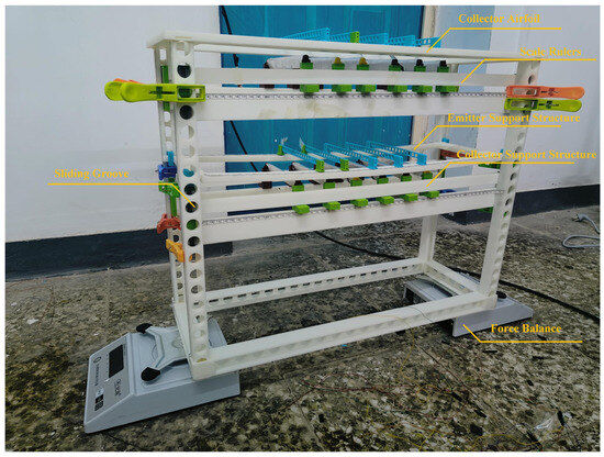
Figure 6.
Customized experimental setup.
As shown in Figure 6, the customized experimental setup was utilized to perform direct thrust and electric field measurements. The device consists of a support framework, a two-stage thruster support structure, and two-stage thrusters. Each thruster stage was composed of five emitters and six collectors arranged in a staggered distribution. The emitters of the first stage were installed at the top of the device. The collectors of the first stage and the electrode assembly of the second stage could slide together within the pillars of the device structure, allowing for adjustments in the electrode gap d and thruster stage spacing θ. To adjust the thruster unit spacing s, the structures supporting both the emitters and the collectors were equipped with grooves that had smooth surfaces, which enabled the sliding blocks used for installing the electrodes to move smoothly within the grooves. Scale rulers were placed near the grooves of the pillars and structures supporting the test device, which facilitated the adjustment of the distance parameters during each sampling. The airfoil collectors and supporting airfoil sliding blocks were connected using quick connectors, allowing for a convenient method to replace the airfoil electrodes after each sampling. The plastic clip was used to fix the position of the three-stage electrode below after adjusting the distance. All components of the experimental setup were fabricated using 3D-printing technology with insulating materials, such as polylactic acid (PLA). The adjustment accuracy for the electrode gap d, the thruster unit spacing s, and the thruster stage spacing θ was 1 mm.
In this study, two precision measurement balances with an accuracy of 0.01 g were symmetrically placed on both sides of the device to prevent downward ion wind from interfering with the measuring instruments. The weight range of each balance was 0–10 kg. To measure the current passing through the thruster, an ammeter that had an accuracy of 1 μA was connected in series between the collector electrode and the ground wire. The experimental procedure was as follows. Firstly, select the airfoil with a corresponding thickness and chord length before the experiment starts, then adjust the three distance parameters for installing the airfoil, and start the experiment. During measurement, fix the power supply voltage at 20 kV. Use the sum force from two balances minus their initial readings as the thrust indication at the current moment. The experiment involves certain uncertainties, which are typically greater when the ion wind is stronger, resulting in more significant fluctuations in balance readings. This uncertainty cannot be precisely measured. So, the experimental procedure involves setting the high voltage to the desired value for 5 s and then recording average data within 30 s to reduce experimental errors. All experiments were conducted at a voltage at 20 kV, a temperature between 19 and 21 °C, an atmospheric pressure between 0.97 and 1.01 bar, and a relative humidity between 28 and 32%. The specific experimental parameters are summarized as shown in Table 3.
Table 3.
Specific experimental parameters.
5. Numerical Results
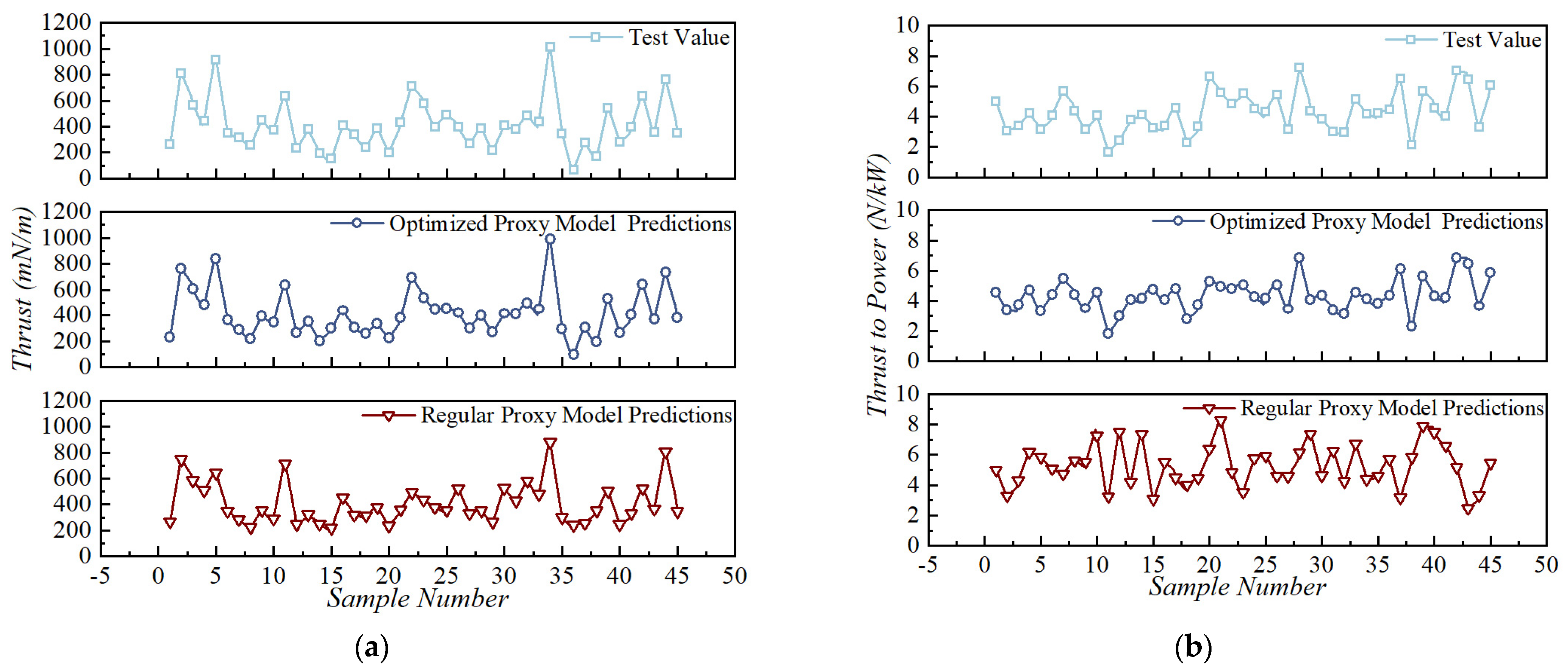
5.1. Evaluation of Proxy Model Accuracy
Based on the sampled dataset, we established a proxy model using the Bayesian regularization BP neural network, which was improved by the genetic algorithm with regularization. To demonstrate the superiority of this proxy-model-building method, we established a basic proxy model using a regular BP neural network. When establishing the proxy model, the average relative error of the predicted values in the test dataset was analyzed to determine the reliability of the established model. Figure 7 compares the actual and predicted values of the proxy model for all samples. The figure shows that both proxy models exhibited superior fitting accuracy when predicting the thrust performance. The basic proxy model did not achieve favorable fitting results for the thrust-to-power ratio, whereas the improved proxy model satisfied all of the requirements.
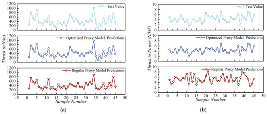
Figure 7.
Comparison between the predictions of the two proxy models and the actual values. (a) comparison of thrust. (b) comparison of thrust to power.
Table 4 shows the predictive accuracy of the proxy model, which was obtained through comparison with the corresponding actual values in the test dataset. The table indicates that the average relative error of the thrust of the proxy model was 3.73%, the average relative error of the thrust-to-power ratio was 3.57%, and the total average relative error of the two output indicators was 3.65%. The expected accuracy of the proxy model had a total average relative error of 5%. Therefore, the fitting accuracy of the proxy model satisfied the predetermined requirements.
Table 4.
Prediction accuracy of the proxy model.
5.2. Influence of the Electrode Gap (d) and the Thruster Unit Spacing (s)
Coseru et al. [33] conducted numerical simulations on EAD thrusters of types 1E/1C, 1E/2C, and NE/NC (i.e., N emitters/N collectors, where N is a positive integer) and analyzed the impact of parameters, such as d and s, on the performance of the thrusters. In contrast, this study focused on sampling and investigating the staggered electrode distribution of 5E/6C. In a numerical study conducted by Coseru et al. [33] on N pairs of emitters and collectors in a collinear distribution, as s increased, the thrust initially increased and subsequently stabilized. This occurred because in the collinear electrode distribution, the distance between the emitters and collectors in the collinear pairs remains unchanged as the spacing s increases. However, the distance between the emitters and collectors of adjacent electrode units increases. Therefore, increasing the spacing s effectively causes the thruster to transition from the NE/NC distribution to the distribution of N pairs of electrodes (1E/1C), thereby reducing the effects of aerodynamic blockage and electrostatic shielding between the electrode units. For the 5E/6C staggered distribution examined in this study, there was no collinear distribution of the emitters and collectors.
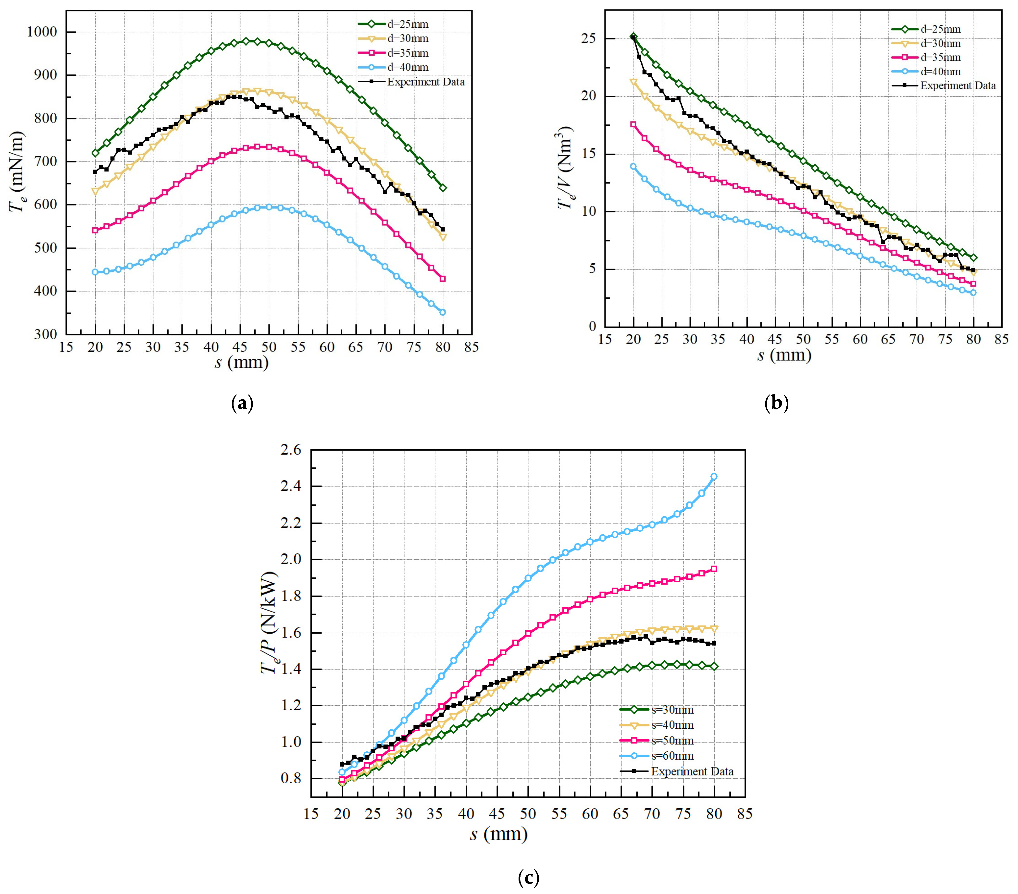
Figure 8 depicts the predicted impact of the spacing s on the performance of the thruster for 20 mm < s < 80 mm and a power supply voltage of 20 kV, θ = 150 mm, t = 10 mm, and c = 30 mm. It also compares the performance curves for different d values of 25, 30, 35, and 40 mm. Furthermore, we designed a set of experimental test data using the controlled variable method, with all parameters matching those of the d = 30 mm group. The results are also shown in Figure 8. From the figure, it was seen that there is an error range of less than 10% between the simulation results and the experimental data, indicating that the simulation model possessed a fairly reliable generalization capability. Due to the similar format of the content in Section 5.2, Section 5.3, and Section 5.4, the comparisons between simulation results and experimental results are not presented in Section 5.3 and Section 5.4 for the purpose of improving readability.
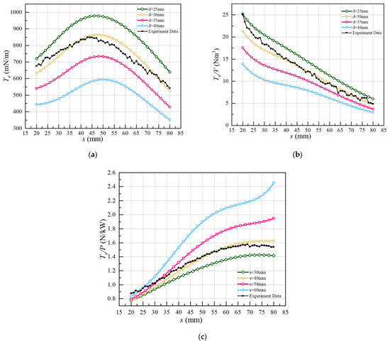
Figure 8.
Prediction of the impact of the thruster unit spacing s on the performance parameters. (a) performance of thrust. (b) performance of thrust density. (c) performance of thrust-to-power.
As shown in Figure 8a, as the spacing s between the electrode units increased, the thrust initially increased and then decreased. The distance between each emitter and collector also increased. When s/d was less than 1.5, the situation was similar to that of the NE/NC case. As s/d increased, the thruster units became decoupled, and the effects of aerodynamic blockage and electrostatic shielding decreased. Consequently, the thrust gradually increased. When s/d was more than 1.5, the thruster units became completely decoupled, and, at this point, the thrust losses caused by aerodynamic blockage and electrostatic shielding effects became increasingly smaller. It should be noted that the equation describing the impact of s/d on thrust may vary to some extent depending on the parameters c and t, so the numbers determined above are not fixed. However, as s/d enlarged, the distance between the emitters and the collectors increased because of the staggered arrangement. This gradually degraded the thrust performance, and, ultimately, at a fixed value of d, there was an s value that produced the maximum thrust.
Figure 8b shows the variation in the thrust density as a function of the spacing s and electrode gap d. As s and d increased, the thrust density gradually decreased. Within the ranges of 20 mm ≤ d ≤ 50 mm and 20 mm ≤ s ≤ 80 mm, the smaller the gap d and spacing s, the higher the thrust density. Thus, for the 5E/6C case, the increase in s was not sufficient to compensate for the increase in the working volume of the thruster.
Figure 8c shows the influence of variations in s and d on the thrust-to-power ratio. Within the range of values used in this study, increasing s and d improved the thrust-to-power ratio of the EAD thruster. For smaller s values, the thrust increased as the s/d ratio increased, which indicated that an increase in s and a decrease in d had similar impacts on the thrust performance of the EAD thruster. This result suggests that s and d have complementary physical properties.
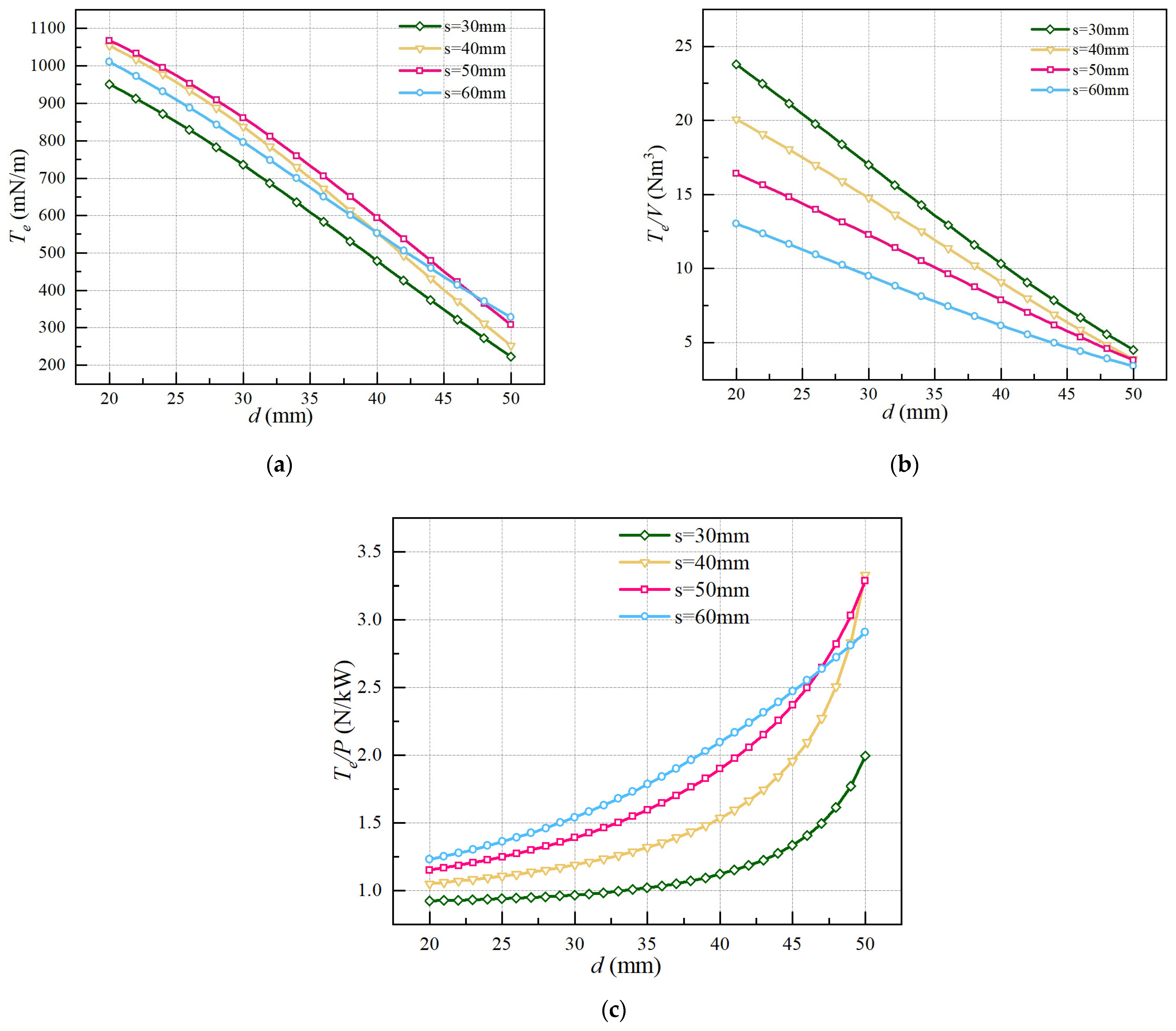
Figure 9 illustrates the predicted impact of the electrode gap d on the performance of the thruster for 20 mm < d < 50 mm and a power supply voltage of 20 kV, θ = 150 mm, t = 10 mm, and c = 30 mm. It also compares the performance curves for different s values of 30, 40, 50, and 60 mm.
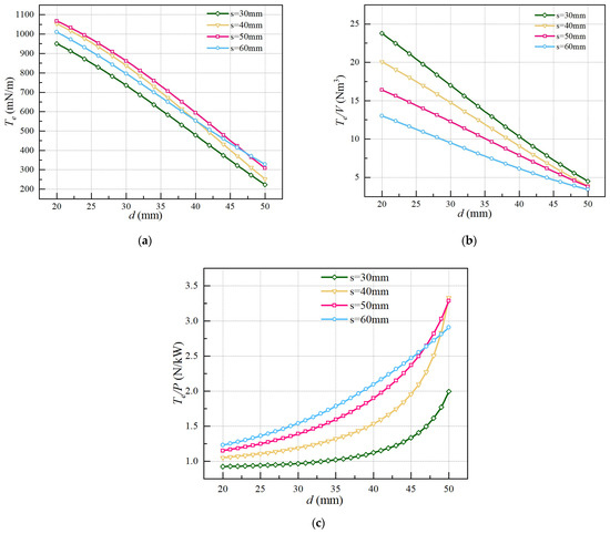
Figure 9.
Prediction of the impact of the electrode gap d on the performance parameters. (a) performance of thrust. (b) performance of thrust density. (c) performance of thrust-to-power.
Figure 9a shows that the thrust decreased as d increased, which is consistent with the inverse relationship described by Equation (11). When the value of d was smaller, the cases with s values of 40 and 50 mm exhibited greater thrust. Figure 9b shows a continuous decrease in the thrust density as d increased. Evidently, the increase in the electrode gap led to a decrease in the thrust and an increase in the working volume. Additionally, a larger spacing s represented a larger working volume, consequently leading to a decrease in the thrust density. Figure 9c shows that the thrust-to-power ratio continued to increase as d and s increased, which is consistent with Equation (12). Because of the leakage current between the thruster electrodes, the slope of the thrust-to-power ratio curve increased with d; at smaller d values, the current was higher, resulting in larger power losses. Additionally, our analysis indicated that as d increased, the influence of the aerodynamic drag gradually decreased, which improved the thrust-to-power ratio.
5.3. Influence of the Thruster Stage Spacing (θ)
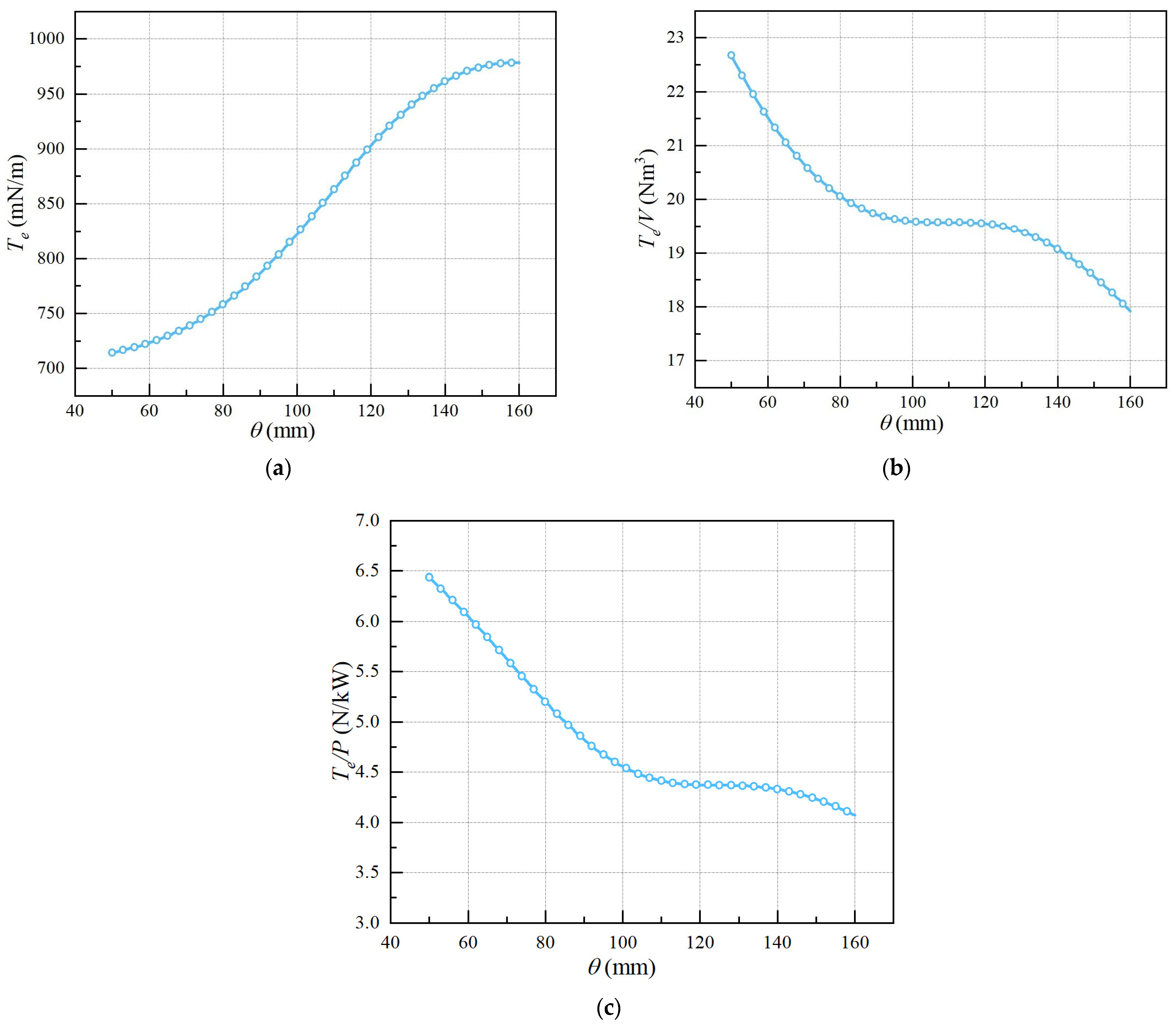
Figure 10 presents the predicted impact of the thruster stage spacing θ on the performance of the thruster for 50 mm ≤ θ ≤ 160 mm and a power supply voltage of 20 kV, d = 20 mm, s = 40 mm, t = 10 mm, and c = 30 mm.
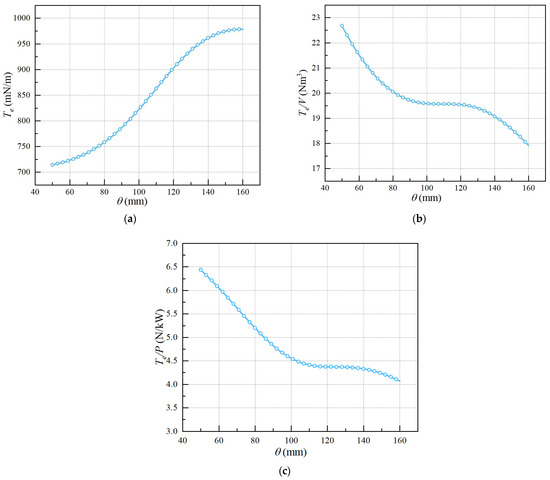
Figure 10.
Prediction of the impact of the thruster stage spacing θ on the performance parameters. (a) performance of thrust. (b) performance of thrust density. (c) performance of thrust-to-power.
Figure 10a indicates that the thrust increased as θ increased. However, the growth rate significantly decreased after θ reached 140 mm. The increase in thrust was due to the gradual reduction in the reverse-discharge between adjacent electrode sets, which reduced the intensity of the reverse-ion wind. When θ was large, the interference from the reverse-discharge was negligible. Therefore, further increasing θ did not have a significant impact on the thrust performance. Figure 10b demonstrates that as θ increased, the thrust density decreased; this trend was the opposite of that of the thrust. Between the endpoints of the θ value range, a flat region occurred, indicating that the optimal value of θ, which balanced both the thrust and the thrust density performance, was likely to be within that region. The characteristics of the specific impulse ratio (Figure 10c) were also similar to those of the thrust density. As θ increased, the specific impulse ratio gradually decreased. In the analysis of the single geometric parameters described above, the trend of the specific impulse ratio was often the opposite of that of the thrust change. This further highlighted the importance of selecting an optimal parameter combination to balance the values of these two factors.
5.4. Influence of the Collector Airfoil Thickness (t) and Chord Length (c)
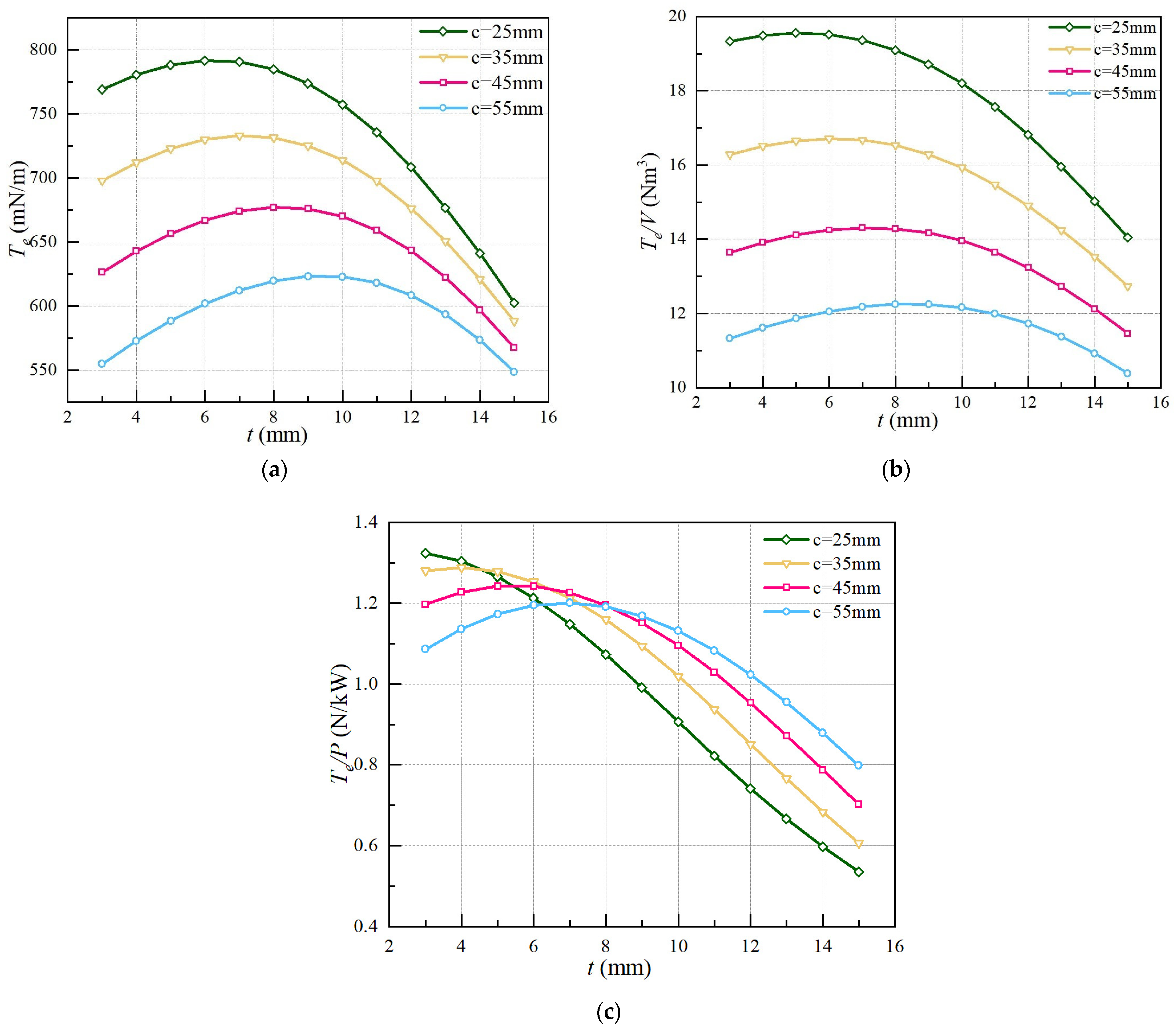
Figure 11 shows the predicted impact of the collector airfoil thickness t on the performance of the thruster for 3 mm ≤ s ≤ 15 mm and a power supply voltage of 20 kV, d = 20 mm, s = 25 mm, and θ = 100 mm. It also compares the performance curves for different c values of 25, 35, 45, and 55 mm.
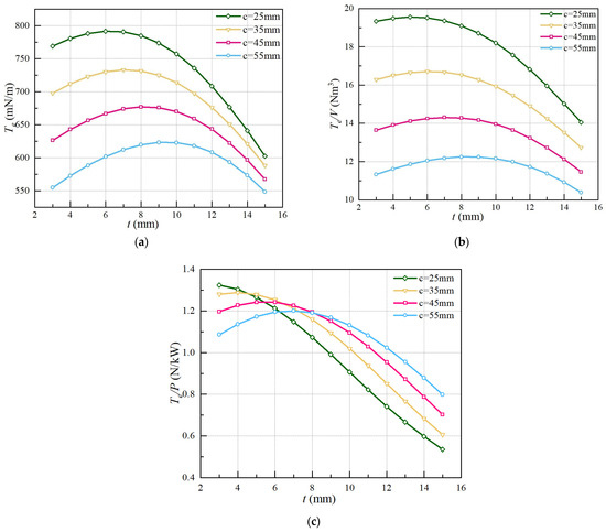
Figure 11.
Prediction of the impact of the collector airfoil thickness t on the performance parameters. (a) performance of thrust. (b) performance of thrust density. (c) performance of thrust-to-power.
Figure 11a indicates that as t increased, the thrust initially increased and then decreased. On the one hand, an increase in the discharge cross-section had a beneficial impact on the electric thrust. On the other hand, an increase in the thickness enhanced the blockage, causing aerodynamic deterioration. The combined effect of these two factors resulted in a local maximum. Figure 9a demonstrates that the smaller the chord length, the larger the thrust. This occurred because an excessively long airfoil introduced a significant amount of parasitic drag owing to friction, which reduced the effective thrust of the EAD thruster. This indicated that increasing the t/c ratio when t was relatively small was beneficial for increasing the effective thrust. In addition, as the chord length decreased, the local maximum for t shifted toward smaller values. This trend reflected the fact that thinner and smaller airfoil profiles were advantageous for increasing the thrust.
Figure 11b shows the variation in the thrust density as a function of t. Because the changes in t and c had minimal impact on the operating range of the thruster, their effects on the thrust density were very similar to those on the thrust. The local maximum thrust density was not significantly different compared to that of the thrust. For optimization, we adopted the approximation that an increase in both t and c led to a decrease in the thrust density.
Figure 11c shows the thrust-to-power ratio as a function of t and c. Because the power of the EAD thruster was less influenced by aerodynamics, increasing the thickness led to an increase in the discharge cross-section, thereby increasing the power. However, the thrust initially increased and then decreased as t increased. Therefore, the thrust-to-power ratio first increased and then decreased as t increased. When t was small, a smaller c value resulted in a larger thrust, resulting in a relatively high thrust-to-power ratio. As t increased by a certain amount, the short chord length compressed the airfoil shape, generating a flattened leading edge and causing the maximum thickness plane to be closer to the emitter. These effects increased the power and caused the thrust-to-power ratio to decrease more rapidly. When t was small, increasing the t/c ratio produced an increase in the thrust, reflecting the similar impacts of increasing t and decreasing c on the thrust performance. This suggested that t and c exhibited complementary physical properties.
5.5. Genetic Algorithm Optimization Solution
To demonstrate the superiority of the Pareto solution set in the NSGA-II genetic algorithm, we first utilized a single-objective genetic algorithm to separately obtain the maximum thrust, the maximum thrust density, the maximum thrust-to-power ratio, and their corresponding combinations of geometric parameters. Compared to the average values of the original samples, the thrust increased by 225.23%, the thrust density increased by 357.14%, and the thrust-to-power ratio increased by 195.31%. The results are summarized in Table 5.
Table 5.
Single-objective genetic algorithm optimization results and their corresponding optimal parameters.
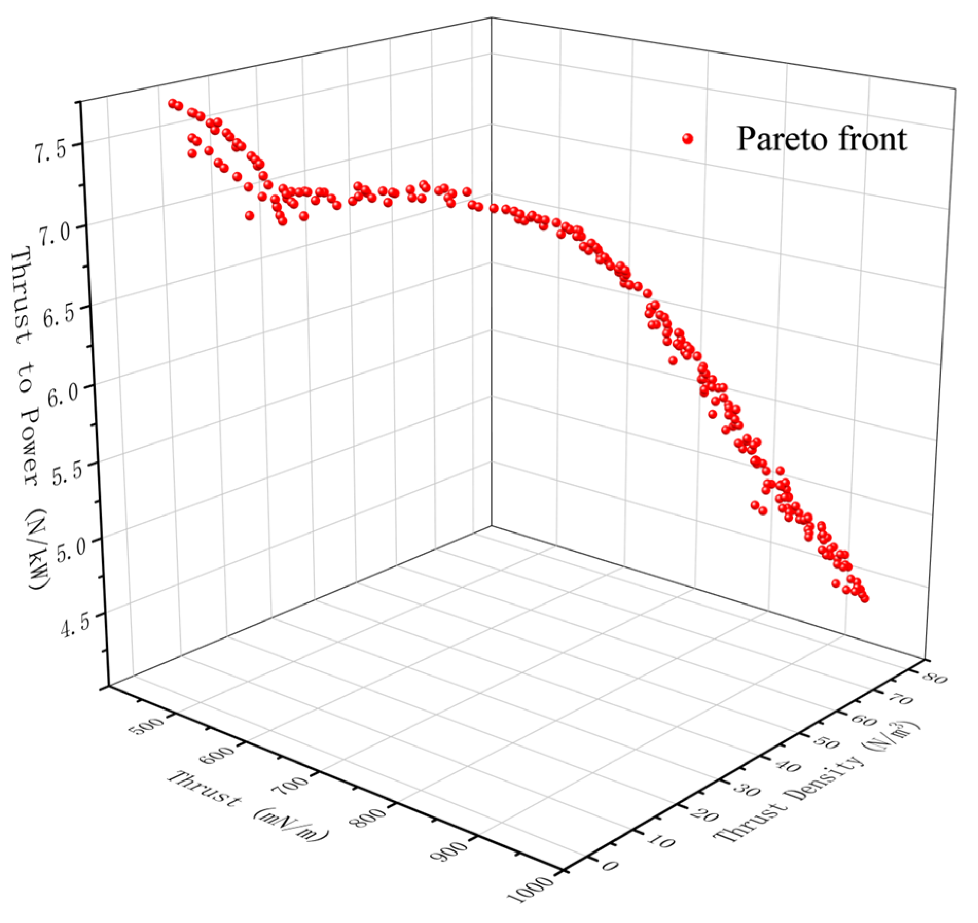
Figure 12 illustrates the Pareto solution set optimized with the NSGA-II multi-objective genetic algorithm. In engineering, where a singular solution is frequently needed, the research developed an evaluation model utilizing the Analytic Hierarchy Process. In this study, the Pareto solution set was normalized according to the three aforementioned optimal performance criteria for an intuitive performance analysis. Through the Analytic Hierarchy Process, seven representative solutions (shown in Table 6) were selected from the generated Pareto solutions to construct a typical Pareto solution set. These selected solutions represented the expected priority solution sets under different weights for thrust, thrust density, and the thrust power ratio.

Figure 12.
The Pareto solution set optimized with the NSGA-II multi-objective genetic algorithm.
Table 6.
Seven representative solutions obtained through the Analytic Hierarchy Process decision-making method.
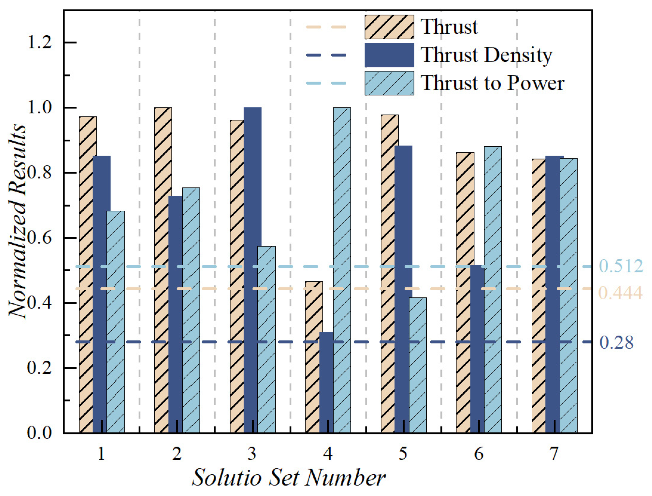
Figure 13 illustrates the normalized performance distribution of the optimized solution sets, with three dashed lines representing the average of the experimental data. Compared to the average of the original data, the optimized solutions exhibited superior performance. And, we analyzed each group of optimal solutions based on the payload capacity and endurance requirements of the drones. If it was necessary to enhance both the payload capacity and the endurance of plasma propulsion drones simultaneously, the seventh solution set could be used. If the goal was to significantly improve the payload capacity at the expense of endurance, the third and fifth solution sets were appropriate. Conversely, if the priority was to enhance endurance while sacrificing payload capacity, the fourth solution set could be adopted. However, it is not recommended to use this method, as the primary issue currently facing plasma propulsion drones is inadequate payload capacity. Additionally, the thrust performance and thrust density of the fourth solution set were significantly subpar. If endurance optimization was required, the sixth and seventh solution sets could be considered as they offered excellent endurance while maintaining good payload capacity. For prioritizing payload capacity improvement while ensuring decent endurance, the first and second solution sets are suggested. In summary, the solutions found in this study represent different performance preferences and could provide greater flexibility and choices for subsequent researchers. They significantly reduced the time spent on designing the thruster geometry, allowing for a focus on other issues related to plasma propulsion drones, such as control.

Figure 13.
The normalized performance distribution of the optimized solution sets.
6. Conclusions
This study predicted and optimized the influence of the main geometric parameters of plasma thrusters on their performance. The main geometric parameters included the electrode gap d, the electrode unit spacing s, the thruster stage spacing θ, the maximum thickness of the collector airfoil t, and the chord length of the collector airfoil c. The staggered distribution was adopted for the thruster’s configuration. The advantages of the staggered distribution in reducing drag were briefly analyzed from an aerodynamic perspective based on the one-dimensional EAD theory. To reduce the experimental and computational costs, a proxy model was established using a BP neural network that was improved via a genetic algorithm. By customizing the measurement of thrust and current, a more detailed analysis of the impact of the EAD thruster performance was carried out based on 45 sets of experimental data. Using the NSGA-II multi-objective genetic algorithm for optimizing the prediction results, we applied the Analytic Hierarchy Process to enhance the Pareto solution set through balancing and selection. This process helped us identify seven geometric parameter combinations with superior overall performance, each reflecting distinct performance preferences. However, this study suffers from a small sample size, insufficient data, and potential biases in the predictions of the experimental setup and proxy models, which have implications and limitations for the conclusions of this paper. In addition, the optimized performance may still not meet the performance requirements of plasma aircrafts.
In the staggered distribution of 5E/6C (five emitters/six collectors), an increase in thrust led to a decrease in the thrust-to-power ratio, which was consistent with the experimental and theoretical results. Within the parameter range investigated in this study, reducing the electrode gap d and the electrode unit spacing s resulted in a higher thrust density; however, increasing both values improved the thrust-to-power ratio. Increasing the thruster stage spacing θ effectively suppressed the generation of a reverse-ion wind, and its impact on the thrust density and thrust-to-power ratio was the opposite of that on the thrust. Thinner and smaller airfoil collector electrodes were beneficial for increasing the thrust. Changing the thickness t and chord length c had a negligible impact on the working volume of the plasma thruster; therefore, the variation in the thrust density followed a trend similar to that of the thrust.
To determine the predicted values of the maximum thrust, the maximum thrust density, and the maximum thrust-to-power ratio, geometric parameter combinations were obtained using a single-objective genetic algorithm. Compared to the average values of the original samples, the thrust increased by 225.23%, the thrust density increased by 357.14%, and the thrust-to-power ratio increased by 195.31%.
The normalized Pareto solution set provided a balanced performance across multiple objectives. Therefore, it discovered a range of solutions that performed well across different objectives rather than optimizing only for a single objective. Using the NSGA-II genetic algorithm to acquire the Pareto optimal solution set, a decision was made utilizing the Analytic Hierarchy Process to pinpoint seven representative optimal parameter combinations. Subsequent researchers could select an appropriate solution based on the drone’s payload capacity and endurance requirements. For instance, the first solution set was suggested for prioritizing payload capacity improvement while ensuring decent endurance. It was beneficial to address the current performance shortcomings of plasma propulsion drones and provide greater flexibility and choice for subsequent researchers.
Follow-up research could focus on the use of more accurate proxy models and experimental data, as well as the use of higher-thrust thruster configurations, such as the multi-staged ducted thrusters proposed by Gomez-Vega [35].
Author Contributions
Conceptualization, Y.Y. (Yulong Ying), T.L. and N.Q.; Methodology, Z.X., T.L., Y.Y. (Yuxuan Yao) and M.H.; Software, Z.X., Y.Y. (Yulong Ying) and H.L.; Validation, Z.X. and H.L.; Writing—original draft, Z.X. and Y.Y. (Yulong Ying); Writing—review & editing, Z.X., Y.Y. (Yulong Ying) and M.H. All authors have read and agreed to the published version of the manuscript.
Funding
This work was supported in part by the National Natural Science Foundation of China (grant number 12272104) and in part by the National Natural Science Foundation of China (grant number U22B2013).
Data Availability Statement
The original contributions presented in the study are included in the article, further inquiries can be directed to the corresponding author.
Conflicts of Interest
The authors declare no conflict of interest.
Appendix A
Table A1.
The 45 sample points selected by the Latin Hypercube design (unit: mm).
Table A1.
The 45 sample points selected by the Latin Hypercube design (unit: mm).
| Sample Number | d | s | θ | c | t | Sample Number | d | s | θ | c | t | Sample Number | d | s | θ | c | t |
|---|---|---|---|---|---|---|---|---|---|---|---|---|---|---|---|---|---|
| 1 | 49 | 47 | 85 | 12.47 | 36.08 | 16 | 30 | 70 | 102 | 14.92 | 37.67 | 31 | 22 | 75 | 64 | 9.45 | 27.97 |
| 2 | 25 | 34 | 148 | 7.36 | 47.49 | 17 | 42 | 65 | 90 | 3.85 | 26.97 | 32 | 20 | 69 | 84 | 13.44 | 30.28 |
| 3 | 26 | 24 | 130 | 9.85 | 56.59 | 18 | 35 | 26 | 66 | 13.16 | 21.23 | 33 | 26 | 53 | 63 | 7.17 | 49.60 |
| 4 | 32 | 73 | 142 | 9.36 | 44.35 | 19 | 37 | 50 | 58 | 3.11 | 31.18 | 34 | 21 | 41 | 135 | 10.78 | 41.35 |
| 5 | 21 | 31 | 98 | 8.47 | 43.28 | 20 | 46 | 40 | 91 | 11.36 | 58.13 | 35 | 40 | 38 | 59 | 13.97 | 48.48 |
| 6 | 41 | 30 | 111 | 6.37 | 46.30 | 21 | 38 | 52 | 62 | 11.55 | 61.10 | 36 | 48 | 65 | 57 | 13.68 | 28.96 |
| 7 | 45 | 63 | 106 | 10.36 | 20.23 | 22 | 29 | 42 | 124 | 8.72 | 50.84 | 37 | 48 | 36 | 121 | 10.56 | 23.16 |
| 8 | 49 | 75 | 95 | 7.86 | 18.37 | 23 | 28 | 44 | 81 | 12.67 | 15.41 | 38 | 36 | 23 | 75 | 14.68 | 62.11 |
| 9 | 33 | 49 | 70 | 5.49 | 53.15 | 24 | 35 | 32 | 139 | 12.98 | 63.74 | 39 | 25 | 68 | 118 | 11.36 | 58.13 |
| 10 | 39 | 62 | 146 | 12.30 | 68.92 | 25 | 33 | 37 | 128 | 10.19 | 65.84 | 40 | 46 | 59 | 86 | 6.98 | 66.47 |
| 11 | 23 | 28 | 109 | 14.46 | 33.44 | 26 | 30 | 20 | 101 | 4.75 | 59.89 | 41 | 41 | 57 | 154 | 5.99 | 42.56 |
| 12 | 34 | 80 | 79 | 3.38 | 68.10 | 27 | 38 | 77 | 59 | 5.23 | 16.57 | 42 | 28 | 46 | 112 | 7.64 | 39.65 |
| 13 | 42 | 55 | 57 | 5.76 | 24.76 | 28 | 43 | 57 | 157 | 4.99 | 35.43 | 43 | 44 | 45 | 148 | 6.48 | 19.06 |
| 14 | 44 | 61 | 67 | 4.08 | 64.93 | 29 | 34 | 78 | 70 | 3.70 | 51.79 | 44 | 24 | 51 | 160 | 9.05 | 32.60 |
| 15 | 47 | 22 | 117 | 11.81 | 38.34 | 30 | 35 | 28 | 150 | 4.35 | 55.55 | 45 | 40 | 71 | 129 | 8.20 | 25.46 |
References
- Cao, W.; Mecrow, B.C.; Atkinson, G.J.; Bennett, J.W.; Atkinson, D.J. Overview of Electric Motor Technologies Used for More Electric Aircraft (MEA). IEEE Trans. Ind. Electron. 2012, 59, 3523–3531. [Google Scholar]
- Xu, H.; He, Y.; Strobel, K.L.; Gilmore, C.K.; Kelley, S.P.; Hennick, C.C.; Sebastian, T.; Woolston, M.R.; Perreault, D.J.; Barrett, S.R.H. Flight of an aeroplane with solid-state propulsion. Nature 2018, 563, 532–539. [Google Scholar] [CrossRef] [PubMed]
- Moreau, E.; Benard, N.; Alicalapa, F.; Douyere, A. Electrohydrodynamic force produced by a corona discharge between awire active electrode and several cylinder electrodes_Application toelectric propulsion. J. Electrost. 2015, 76, 194–200. [Google Scholar] [CrossRef]
- Brown, T.T. A Method of and an Apparatus or Mechine for Producing Force or Motion. UK Patent No. 300.311, 15 August 1928. [Google Scholar]
- Robinson, M. Movement of air in the electric wind of the corona discharge. Trans. Am. Inst. Electr. Eng. Part I Commun. Electron. 1961, 80, 143–150. [Google Scholar] [CrossRef]
- Stuetzer, O.M. Ion Drag Pumps. J. Appl. Phys. 1960, 31, 136–146. [Google Scholar] [CrossRef]
- Sun, Z.; Velasquez-Garcia, L.F. Multiplexed Electrohydrodynamic Gas Pumps. Plasma Res. Express 2020, 2, 9–25. [Google Scholar] [CrossRef]
- Roth, J.R. Aerodynamic Flow Acceleration Using Paraelectric and Peristaltic Electrohydrodynamic Effects of a One Atmosphere Uniform Glow Discharge Plasma. Phys. Plasmas 2003, 10, 2117–2126. [Google Scholar] [CrossRef]
- Moreau, E. Airflow Control by Non-Thermal Plasma Actuators. J. Phys. D Appl. Phys. 2007, 40, 605–636. [Google Scholar] [CrossRef]
- Yamamoto, T.; Velkoff, H.R. Electrohydrodynamics in an Electrostatic Precipitator. J. Fluid Mech. 1981, 108, 1–18. [Google Scholar] [CrossRef]
- Davis, J.L.; Hoburg, J.F. Wire-Duct Precipitator Field and Charge Computation Using Finite Element and Characteristics Methods. J. Electrost. 1983, 14, 187–199. [Google Scholar] [CrossRef]
- Wilson, J.; Perkins, H.D.; Thompson, W.K. An Investigation of Ionic Wind Propulsion; National Aeronautics and Space Administration: Washington, DC, USA, 2009.
- Pekker, L.; Young, M. Model of Ideal Electrohydrodynamic Thruster. J. Propuls. Power 2011, 27, 786–792. [Google Scholar] [CrossRef]
- Johnson, I.K.; Winglee, R.M.; Race Roberson, B. Pulsed plasma thrusters for atmospheric operation. In Proceedings of the 50th AIAA/ASME/SAE/ASEE Joint Propulsion Conference, Cleveland, OH, USA, 28–30 July 2014. [Google Scholar]
- van Wynsberghe, E.; Turak, A. Station-keeping of a high-altitude balloon with electric propulsion and wireless power transmission: A concept study. Acta Astronaut. 2016, 128, 616–627. [Google Scholar] [CrossRef]
- Drew, D.S.; Lambert, N.O.; Schindler, C.B.; Pister, K.S.J. Toward Controlled Flight of the Ionocraft: A Flying Microrobot Using Electrohydrodynamic Thrust with Onboard Sensing and No Moving Parts. IEEE Robot. Autom. Lett. 2018, 3, 2807–2813. [Google Scholar] [CrossRef]
- Zubrin, R.M. In-atmosphere electrohydrodynamic propulsion aircraft with wireless supply onboard. J. Electrost. 2018, 95, 1–12. [Google Scholar]
- Ieta, A.; Chirita, M. Electrohydrodynamic propeller for in-atmosphere propulsion; rotational device first flight. J. Electrost. 2019, 100, 103–352. [Google Scholar] [CrossRef]
- He, Y.; Woolston, M.; Perreault, D. Design and implementation of a lightweight high-voltage power converter for electro-Aerodynamic propulsion. In Proceedings of the 2017 IEEE 18th Workshop on Control and Modeling for Power Electronics, COMPEL 2017, Stanford, CA, USA, 9–12 July 2017. [Google Scholar]
- Zhao, Z.; Zhu, J.; Dai, Y.-X.; Wang, J.; Yang, Y.; Peng, Z.; Xu, Q.; Ning, Y.; He, S. Lightweight Design of Magnetic Integrated Transformer for High Voltage Power Supply in Electro-Aerodynamic Propulsion System. IEEE Trans. Power Electron. 2023, 38, 10501–10515. [Google Scholar] [CrossRef]
- He, Y.; Perreault, D.J. Lightweight High-Voltage Power Converters for Electroaerodynamic Propulsion. IEEE J. Emerg. Sel. Top. Ind. Electron. 2021, 2, 453–463. [Google Scholar] [CrossRef]
- Moreau, E.; Benard, N.; Lan-Sun-Luk, J.-D.; Chabriat, J.-P. Electrohydrodynamic force produced by a wire-to-cylinder dc corona discharge in air at atmospheric pressure. J. Phys. D Appl. Phys. 2013, 46, 204–475. [Google Scholar] [CrossRef]
- Masuyama, K.; Barrett, S.R.H. On the performance of electrohydrodynamic propulsion. Proc. R. Soc. A Math. Phys. Eng. Sci. 2013, 469, 2154. [Google Scholar] [CrossRef]
- Gilmore, C.K.; Barrett, S.R.H. Electrohydrodynamic thrust density using positive corona-induced ionic winds for in-Atmosphere propulsion. Proc. R. Soc. A Math. Phys. Eng. Sci. 2015, 471, 2175. [Google Scholar] [CrossRef]
- Monrolin, N.; Plouraboue, F.; Praud, O. Electrohydrodynamic thrust for in-atmosphere propulsion. AIAA J. 2017, 55, 4296–4305. [Google Scholar] [CrossRef]
- Belan, M.; Arosti, L.; Polatti, R.; Maggi, F.; Fiorini, S.; Sottovia, F. A parametric study of electrodes geometries for atmospheric electrohydrodynamic propulsion. J. Electrost. 2021, 113, 103–616. [Google Scholar] [CrossRef]
- Belan, M.; Terenzi, R.; Trovato, S.; Usuelli, D. Effects of the emitters density on the performance of an atmospheric ionic thruster. J. Electrost. 2022, 120, 103–767. [Google Scholar] [CrossRef]
- Zhu, H.; Li, D.; Nie, H.; Wei, X.; Wei, Y. Multiobjective optimization of a staggered-rotor octocopter design based on a surrogate model. Aerosp. Sci. Technol. 2023, 139, 108–387. [Google Scholar]
- Loeb, L.B. Electrical Coronas, Their Basic Physical Mechanisms; University of California Press: Berkeley, CA, USA, 1965. [Google Scholar]
- Liu, J.; Chen, R.; Lou, J.; Hu, Y.; You, Y. Deep-learning-based aerodynamic shape optimization of rotor airfoils to suppress dynamic stall. Aerosp. Sci. Technol. 2023, 133, 108089. [Google Scholar] [CrossRef]
- Huang, J.; Yao, W.X. Multi-objective design optimization of blunt body with spike and aerodisk in hypersonic flow. Aerosp. Sci. Technol. 2019, 93, 105–122. [Google Scholar] [CrossRef]
- He, H.; Shi, P.; Zhao, Y. Adaptive connected hierarchical optimization algorithm for minimum energy spacecraft attitude maneuver path planning. Astrodynamics 2023, 7, 197–209. [Google Scholar] [CrossRef]
- Baklacioglu, T. Modeling the fuel flow-rate of transport aircraft during flight phases using genetic algorithm-optimized neural networks. Aerosp. Sci. Technol. 2016, 49, 52–62. [Google Scholar] [CrossRef]
- Xing, Y.; Tong, L. Accelerating reliability-based topology optimization via gradient online learning and prediction. Aerosp. Sci. Technol. 2024, 145, 108–836. [Google Scholar] [CrossRef]
- Coseru, S.; Fabre, D.; Plouraboue, F. Numerical study of ElectroAeroDynamic force and current resulting from ionic wind in emitter/collector systems. J. Appl. Phys. 2021, 129, 103–304. [Google Scholar] [CrossRef]


Disclaimer/Publisher’s Note: The statements, opinions and data contained in all publications are solely those of the individual author(s) and contributor(s) and not of MDPI and/or the editor(s). MDPI and/or the editor(s) disclaim responsibility for any injury to people or property resulting from any ideas, methods, instructions or products referred to in the content. |
© 2024 by the authors. Licensee MDPI, Basel, Switzerland. This article is an open access article distributed under the terms and conditions of the Creative Commons Attribution (CC BY) license (https://creativecommons.org/licenses/by/4.0/).