Enhanced Computational Biased Proportional Navigation with Neural Networks for Impact Time Control

Abstract

Advanced computational methods are being applied to address traditional guidance problems, yet research is still ongoing regarding how to utilize them effectively and scientifically. A numerical root-finding method was proposed to determine the bias in biased proportional navigation to achieve the impact time control without time-to-go estimation. However, the root-finding algorithm in the original method might experience efficiency and convergence issues. This paper introduces an enhanced method based on neural networks, where the bias is directly output by the neural networks, significantly improving computational efficiency and addressing convergence issues. The novelty of this method lies in the development of a reasonable structure that appropriately integrates off-the-shelf machine learning techniques to effectively enhance the original iteration-based methods. In addition to demonstrating its effectiveness and performance of its own, two comparative scenarios are presented: (a) Evaluate the time consumption when both the proposed and the original methods operate at the same update frequency. (b) Compare the achievable update frequencies of both methods under the condition of equal real-world time usage.

1. Introduction

For the design of guidance systems, synchronizing the arrival of multiple vehicles at a target has been receiving increasing attention in recent years. This is because the coordination of multiple vehicles is essential for many applications for strategic purposes, such as missile defense, autonomous vehicles, swarm robotics, and rendezvous of spacecraft [1,2,3,4,5]. The joint efforts of multiple vehicles can significantly enhance the overall performance and robustness of the system in comparison to non-cooperative individuals. Achieving these goals requires precise control of arrival times. It is often termed as the impact time control problem in the guidance field. Efforts have been made towards developing guidance systems that are capable of manipulating the (remaining) time-to-go to the target. A class of approaches parameterize relevant variables dependent on time and shape their time behavior to achieve the desired impact time [6,7,8,9]. Another class of approaches directly controls the time-to-go, utilizing its estimation [10,11,12,13]. Proportional navigation (PN) has been widely used in guidance systems due to its elegant simplicity and robustness. There are also variants of PN proposed to address the impact time control problem [14,15,16,17,18]. One of the most well-known variants is the biased proportional navigation (BPN) guidance law, which adds a bias term to the traditional PN guidance law. The BPN structure has long been exploited in this regard [19].

In one of the latest works, a BPN guidance has been proposed [20]. This new BPN guidance method utilizes a numerical root-finding process to determine the bias needed for the desired impact time, thus eliminating the need for continual estimation of the time-to-go. This philosophy was exploited to construct a computational guidance law that remained effective in more challenging scenarios, namely, against moving and maneuvering targets. The root-finding process is iteratively run when the guidance law is used against non-stationary targets, adjusting the bias based on the real-time engagement geometry. The method was shown to be effective in guiding the pursuer to the non-stationary target at the desired impact time while maintaining the simplicity and efficiency of the traditional PN guidance. However, the root-finding algorithm, being the backbone of the original algorithm, inherently has potential drawbacks in numerical efficiency and convergence.

Machine learning-based approaches have recently been widely accepted as solutions to autonomous guidance problems in a variety of domains with enhanced performance [21,22,23,24,25]. The novelty of this paper lies not in proposing sophisticated machine learning algorithms to address guidance problems but rather in the strategic use of simple, efficient methods to improve existing algorithms without introducing new compromises or issues. Specifically, the method proposed in this paper is a direct enhancement of our previous work [20]. The proposed method utilizes a neural network to output the bias directly, which significantly improves the computational efficiency and eliminates the convergence issue of the original method. The neural network is trained using a dataset generated by the original method. The proposed method is expected to offer similar performance to the original method in terms of impact time control, while significantly improving the computational efficiency and convergence performance.

The proposed method also contributed to the structural use of machine learning techniques in the guidance field. In the literature, guidance commands can be directly generated from learning-based methods, e.g., using reinforcement learning to output the control commands [26,27,28]. In this regard, the proposed approach is expected to be more acceptable in the aerospace industry. This is because it uses a simple machine learning approach to enhance a traditional guidance law with proven stability, which is already well established and widely applied. The advantage gained precisely addresses the concerns of the previous variant in [20].

This paper is structured to first introduce the guidance scenario in Section 2, where the technical details of the original BPN guidance law are presented. Section 3 presents the proposed method and the corresponding simulation results are given Section 4. Section 5 concludes this paper.

2. Preliminaries

This section first presents the engagement scenario and the geometric relationship between the pursuer and the target. Then, the original BPN guidance law is briefly reviewed. The content of this section, for its introductory nature, is practically modified from our previous work [20].

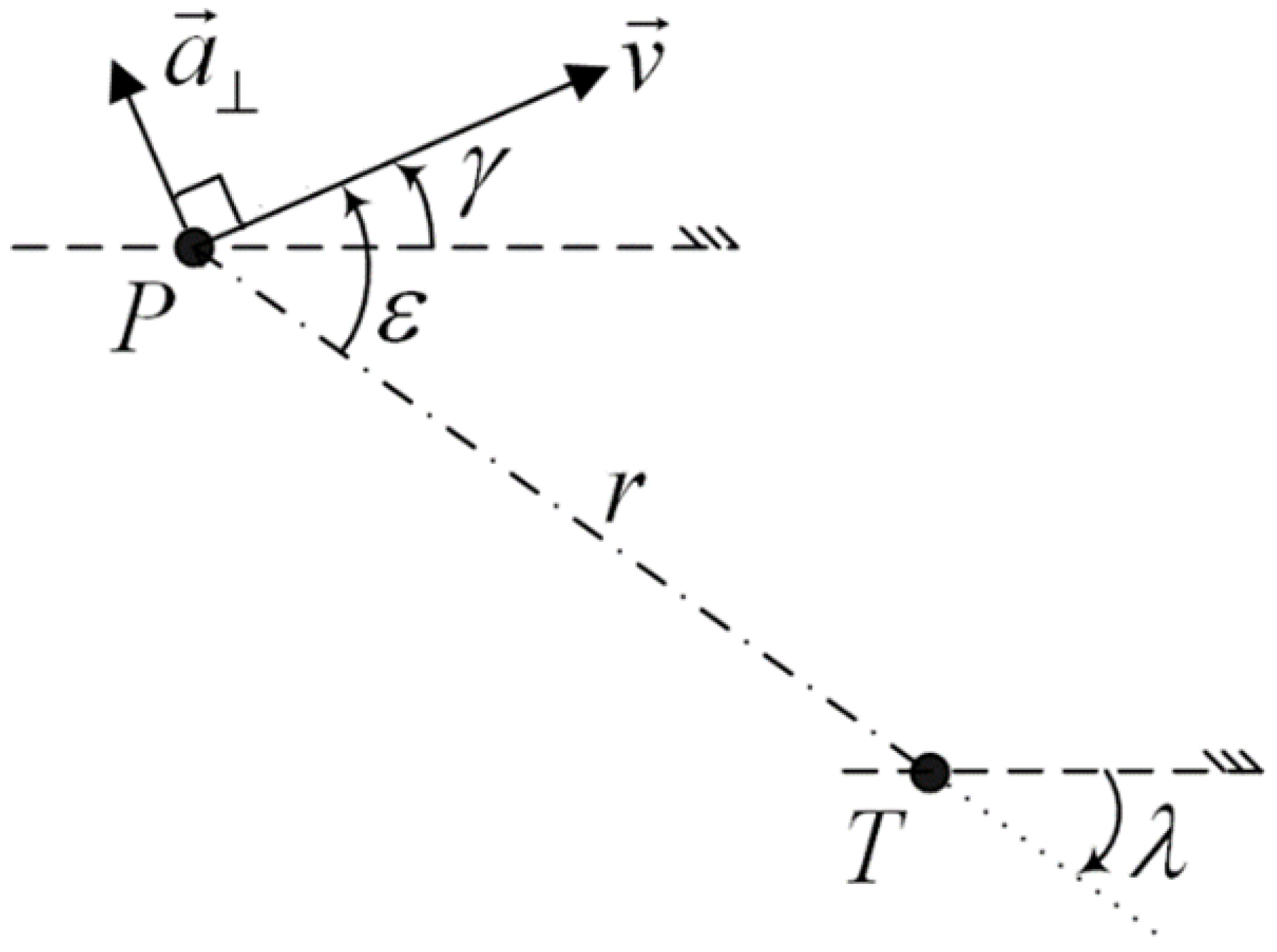
2.1. Engagement Geometry

The focused engagement geometry is a classical two-dimensional engagement scenario. The engagement geometry between the pursuer P and the target T is depicted in Figure 1. The relative range is denoted by r. The look angle, line-of-sight angle, and flight path angle are represented by $ϵ$, $\lambda$, and $\gamma$, respectively. The speed of the pursuer is indicated by V. The pursuer is controlled by the lateral acceleration $a_{\perp }=V\gamma$ perpendicular to its velocity vector. The equations of motion governing the geometry are as follows:

$$\begin{array}{cc}\hfill \dot{r}& =-Vcos(ϵ)\hfill \\ \hfill r\dot{\lambda }& =-Vsin(ϵ)\hfill \end{array}$$

(1)

Additionally, the geometric relationship can be expressed as follows:

$$\lambda =\gamma -ϵ$$

(2)

In this geometry, the target appears to be stationary, while this is not necessarily true. This is used to simplify the guidance design when only lateral acceleration is available. In the opposite case, the ideal PN can be employed where translational acceleration can be accounted for, and one can refer to the original work for this [20].

2.2. Original Guidance Law

This section recaps the fundamentals of the BPN guidance law introduced in [20], which is referred to as the “original” BPN throughout this paper. The philosophy of the original BPN is to add a bias term to the traditional PN guidance law. The (pure) PN guidance law in a plane is given by the following:

$$a_{\perp }=N\dot{\lambda }V$$

(3)

where N is the navigation gain, describing the proportional relationship between the rotational rate of the pursuer’s velocity vector and the line-of-sight angle as

$$\dot{\gamma }=N\dot{\lambda }$$

(4)

The BPN guidance law incorporates a biased term appended to the right-hand side, as follows:

$$\dot{\gamma }=N\dot{\lambda }+b$$

(5)

where b is the bias. Note that $a_{\perp }=V\dot{\lambda }$ also applies to Equation (5) for computing the acceleration command. The bias is leveraged to achieve specific guidance objectives such as impact angle and/or impact time. To enhance our understanding of BPN kinematics, non-dimensional time and range are introduced as follows:

$$\tau =\sigma bt$$

(6a)

$$\rho ={\displaystyle \frac{\sigma b}{V}}r$$

(6b)

where $\sigma$ indicates the sign of b. By combining Equations (3), (6) and (7), Equation (1) may be written as follows:

$${\rho }^{\prime }=-cos(ϵ)$$

(7a)

$${ϵ}^{\prime }=-\left(N-1\right){\displaystyle \frac{sin(ϵ)}{\rho }}+\sigma$$

(7b)

where ${(·)}^{\prime }=d(·)/d\tau$. For the analytical examination of the look angle, Equation (7b) is divided by Equation (7a):

$${\displaystyle \frac{dsin(ϵ)}{d\rho }}=\left(N-1\right){\displaystyle \frac{sin(ϵ)}{\rho }}-\sigma$$

(8)

The stability aspects of BPN can be found in [29]. The solution for $N\ne 2$ is

$$sin(ϵ)=c{\rho }^{N-1}+{\displaystyle \frac{\sigma }{N-2}}\rho$$

(9)

Given the initial range and look angle, the integration constant c for a given bias can be obtained as

$$c=\left(sin({ϵ}_i)-{\displaystyle \frac{\sigma {\rho }_i}{N-2}}\right){\rho }_i^{1-N}$$

(10)

where the subscript i denotes the initial value. Furthermore, combining Equations (2), (5), (6a), (7b) and (9) results in

$${\gamma }^{\prime }=-cN{\rho }^{N-2}-{\displaystyle \frac{2\sigma }{N-2}}$$

(11)

Assuming $ϵ\le {\displaystyle \frac{\pi }{2}}$ imposes a realistic seeker limit, implying from Equation (7a) that the range will decrease monotonously. Consequently,

$${\displaystyle \frac{d{\gamma }^{\prime }}{d\rho }}=-cN\left(N-2\right){\rho }^{N-3}$$

(12)

reveals that ${\gamma }^{\prime }$ will also vary monotonously, as will the acceleration according to $a_{\perp }=V\dot{\gamma }$. Thus, the extreme value of the acceleration will occur either at the beginning or the end of the engagement. The terminal “jerk” is given by

$$\underset{\rho \to 0}{lim}{\displaystyle \frac{d{\gamma }^{\prime }}{d\rho }}=\left\{\begin{array}{cc}0\hfill & \mathrm{if}N\ge 3\hfill \\ \pm \infty \hfill & \mathrm{otherwise}\hfill \end{array}\right.$$

(13)

This indicates that $N<3$ is unsuitable for BPN. Regarding the initial and terminal accelerations, going one step back from Equation (11) via Equation (9) and then returning to the dimensional variables using Equation (6) can simply be written as follows:

$$a_i=-NVsin({ϵ}_i)+bV$$

(14a)

$$a_f=-{\displaystyle \frac{2bV}{N-2}}$$

(14b)

Next, the relation between the desired impact time and the bias is derived. This relation is solved for the bias through a root-finding process. The philosophy of obtaining the relation is to make use of the initial and terminal conditions. The initial conditions ${\gamma }_i$, ${\lambda }_i$, and ${ϵ}_i$ are fully known, while the terminal conditions are unclear. To avoid integration over time, the change rate of the flight path angle is expressed with respect to the non-dimensional range $\rho$. Using the chain rule and considering Equations (7a), (9) and (11), we get the following:

$${\displaystyle \frac{d\gamma }{d\rho }}={\displaystyle \frac{d\gamma }{d\tau }}{\displaystyle \frac{d\tau }{d\rho }}={\displaystyle \frac{Nsin\epsilon /\rho -\sigma }{\sqrt{1-{sin}^2\epsilon }}}=g(\rho )$$

(15)

where $g(\rho )$ since $ϵ=ϵ(\rho )$, as indicated in Equation (9). Assuming a successful engagement, the terminal path angle is given by the definite integral of Equation (15):

$${\gamma }_f={\gamma }_i+{\int }_0^{{\rho }_i}g(\theta )d\theta$$

(16)

where $\theta$ is a dummy variable. Next, ${\gamma }_f$ is expressed in terms of the desired final time, given by the integrated form of Equation (5):

$${\gamma }_f-{\gamma }_i=N({\gamma }_f-{\lambda }_i)+b{t}_f$$

(17)

Here, it is assumed that the final look angle is zero, i.e., ${\lambda }_f={\gamma }_f$. Combining Equations (2), (16) and (17), we get the following:

$$f=N{ϵ}_i+(N-1){\int }_{{\rho }_i}^{0}g(\theta )d\theta +b{t}_f$$

(18)

The root of f provides the desired bias term b, which leads to the desired impact time. Given a desired impact time and initial conditions, a numerical method, e.g., Newton’s method utilizing the gradient, can be used to find the root of Equation (18). To this end, its derivative with respect to b is computed as

$${\displaystyle \frac{df}{db}}=(N-1){\displaystyle \frac{d}{db}}{\int }_{{\rho }_i}^{0}g(\theta )d\theta +t_f$$

(19)

Using the Leibniz integral rule, Equation (19) is further deduced as

$${\displaystyle \frac{df}{db}}=(N-1)\left(-g({\rho }_i){\displaystyle \frac{\partial {\rho }_i}{\partial b}}+{\int }_{{\rho }_i}^0{\displaystyle \frac{\partial g(\theta )}{\partial b}}d\theta \right)+t_f$$

(20)

where the partial derivative ${\displaystyle \frac{\partial g(\theta )}{\partial b}}$ can be expressed by

$${\displaystyle \frac{\partial g(\theta )}{\partial b}}={\displaystyle \frac{\partial g(\theta )}{\partial sin(ϵ)}}{\displaystyle \frac{\partial sin(ϵ)}{\partial c}}{\displaystyle \frac{\partial c}{\partial {\rho }_i}}{\displaystyle \frac{\partial {\rho }_i}{\partial b}}$$

(21)

The partial derivatives in Equation (21) can be readily obtained via Equations (15), (9), (10) and (6b), respectively:

$${\displaystyle \frac{\partial g(\theta )}{\partial sin(ϵ)}}={\displaystyle \frac{N/\rho -\sigma sin(ϵ)}{{(1-{sin}^2(ϵ))}^{3/2}}}$$

(22)

$${\displaystyle \frac{\partial sin(ϵ)}{\partial c}}={\rho }^{N-1}$$

(23)

$${\displaystyle \frac{\partial c}{\partial {\rho }_i}}=\sigma {\rho }_i^{1-N}\left(1-N\right)sin({ϵ}_i){\rho }_i^{-N}$$

(24)

$${\displaystyle \frac{\partial {\rho }_i}{\partial b}}={\displaystyle \frac{\sigma r_i}{V}}$$

(25)

For solving b from Equation (18), three parameters need to be known: ${ϵ}_i$, $r_i$, and $t_f$. Here, $t_f$ is the desired impact time.

3. Real-Time Bias Computation by Neural Network

According to previous derivations, the relation between the guidance law bias term b and the desired impact time $t_f$ has been incorporated into Equation (1). Thus, the bias b can be solved from this equation with partial derivatives, which will lead to the desired final time $t_f$.

In the original method, Newton’s method is utilized to find the root of Equation (18). Newton’s method is of an iterative nature and might be challenging to converge in some cases. Specifically, the finite integral in Equation (18) potentially consumes the computational power considerably in many iterations. In view of this, we turn to the neural network to accelerate the determination of the bias while preserving competitive precision. To this end, we replace the numeric iterations with an end-to-end map. The neural network takes the actual range r, the relative velocity $v_R$, the look angle ${\epsilon }_R$, the initial guess $b_i$, the navigation gain N, and the expected impact time $t_f$ as inputs. Then, bias will be produced as the output. We implement this neural network by a multi-layer perceptron (MLP) with 128-64 nodes for two hidden layers.

3.1. Neural Network Settings and Dataset Generation

We generate the training set from the closed-loop simulation, where the bias is solved by Newton’s method for each time stamp. In our simulation, we assign the relative velocity $v_R=250\mathrm{m}/\mathrm{s}$, navigation gain $N=4$, and desired impact time $t_f=30\mathrm{s}$ as constants, while the other states, including r and ${\epsilon }_R$, are sampled every 0.03 s. Then, these inputs, for example, ${\{x_i\}}_{i=1}^n$, are normalized by ${\{{\overline{x}}_i\mid {\overline{x}}_i={\displaystyle \frac{x-x_{min}}{x_{max}-x_{min}}}\}}_{i=1}^n$ independently. Eventually, we gathered 1000 samples and randomly selected 80 percent of them as the training set, while others were left for testing.

The objective of the proposed method is to provide an efficient but effective way to upgrade the original method within the well-established BPN framework. No sophisticated neural network architecture is required, and the training set can be easily generated from the original method. The philosophy is ultimately straightforward, and the philosophy is not limited to the specific simulation case presented in the later section. The generalization of implementing this philosophy can be easily justified because a specific model’s range and speed are determined by design. One can already estimate the minimum and maximum reaching distance and look angle (e.g., $\pm 90°$) to build the training set when a pursuer is chosen. Once the model is set, the training set can be generated by using the model. The neural network can be trained and tested in a similar way as presented in this paper. Thus, the proposed impact time control guidance method can be easily implemented in practice.

3.2. Neural Network Training and Evaluation

The neural network is trained using PyTorch for a total of 200 epochs, which have been carefully selected to guarantee that the model reaches convergence without experiencing overfitting. To achieve a balance between training stability and computational efficiency, a batch size of 64 is employed. The Adam optimizer is utilized to modify the weights of neural networks. The initial learning rates are set to ${10}^{-3}$, the beta values are ${\beta }_1=0.9$ and ${\beta }_2=0.999$, and an epsilon value of ${10}^{-8}$ is employed to avoid division by zero. In addition, we implement a learning rate scheduler that decreases the learning rate by a factor of 0.8 after every 50 epochs in the absence of any improvement in validation loss. To address overfitting, we implement regularization by utilizing dropout with a rate of 0.2 during the training process. To enhance the resilience of the model, the training data are reinforced through the injection of noise, specifically by introducing Gaussian noise to the input data.

The performance of the neural networks is evaluated by substituting the traditional solution for the guidance law bias b with the predictions of neural networks. To ensure consistency, the input data are standardized using the same mean and standard deviation as those used during the training phase. The overall guidance effectiveness of the system is evaluated by computing the average root mean square error (RMSE) throughout multiple simulations. This evaluation specifically considers five important states: downrange and crossrange trajectories, range, look angle, and acceleration.

4. Simulations

This section presents the simulation results of applying the proposed guidance approach. It should be pointed out that comparisons with other guidance approaches have already been addressed in a previous work [20], making it unnecessary to repeat them in this paper, as the proposed approach is a direct upgrade of the original method.

The simulation studies are conducted in a Simulink environment with a AMD Ryzen 7 5800H 3.20 GHz (AMD, Santa Clara, CA, USA), which is a rather powerful platform in comparison to the actual hardware onboard. The engagement involves a pursuer moving at 250 m/s toward its target positioned 5 km away from the starting point.

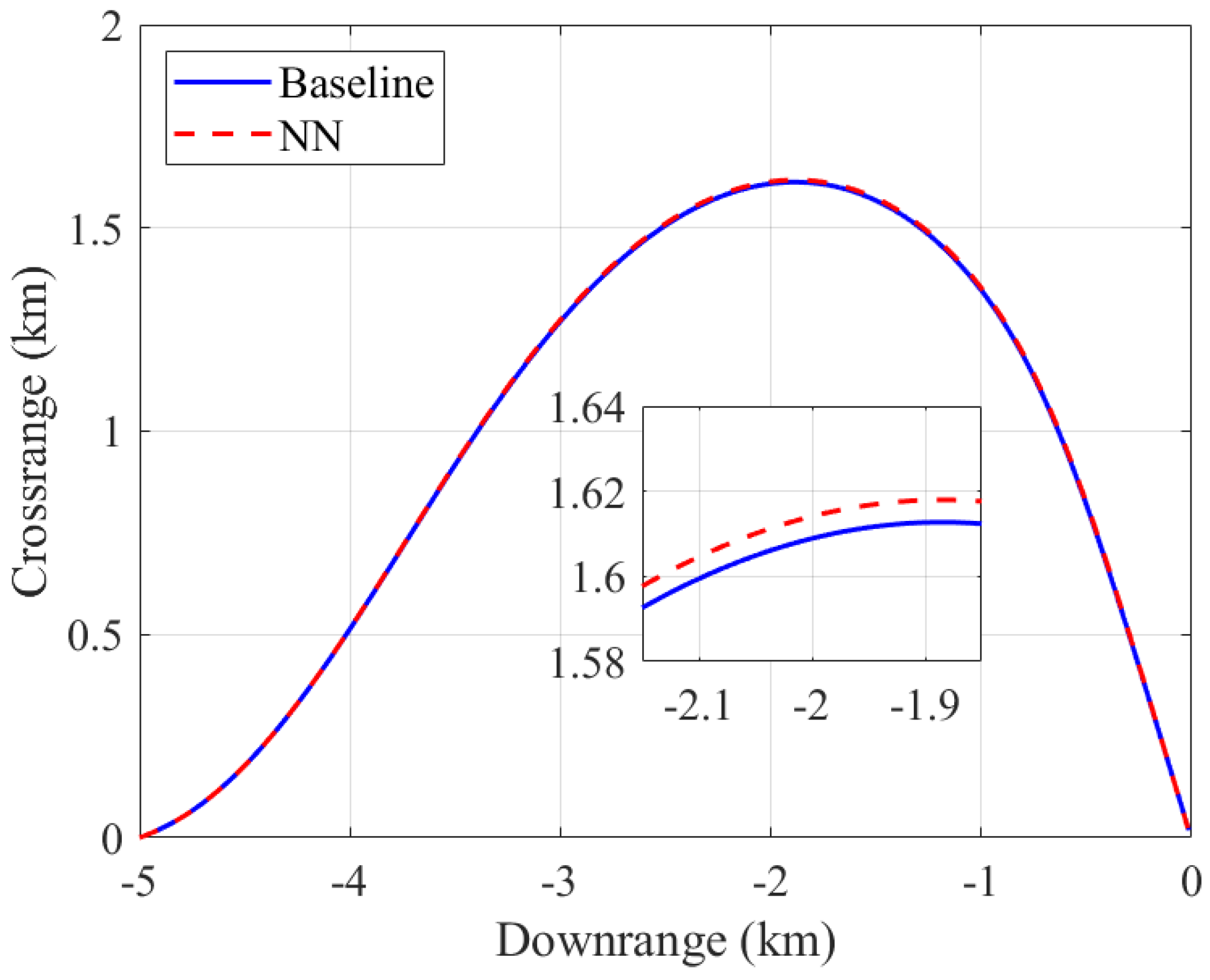
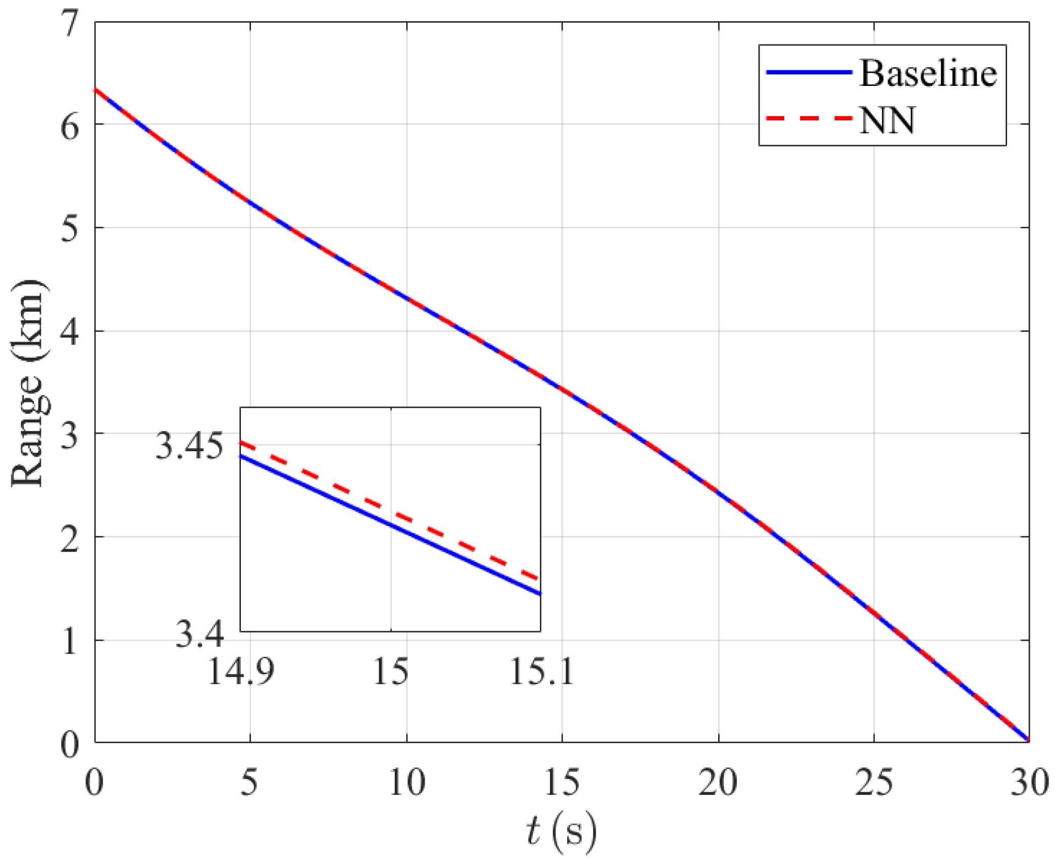
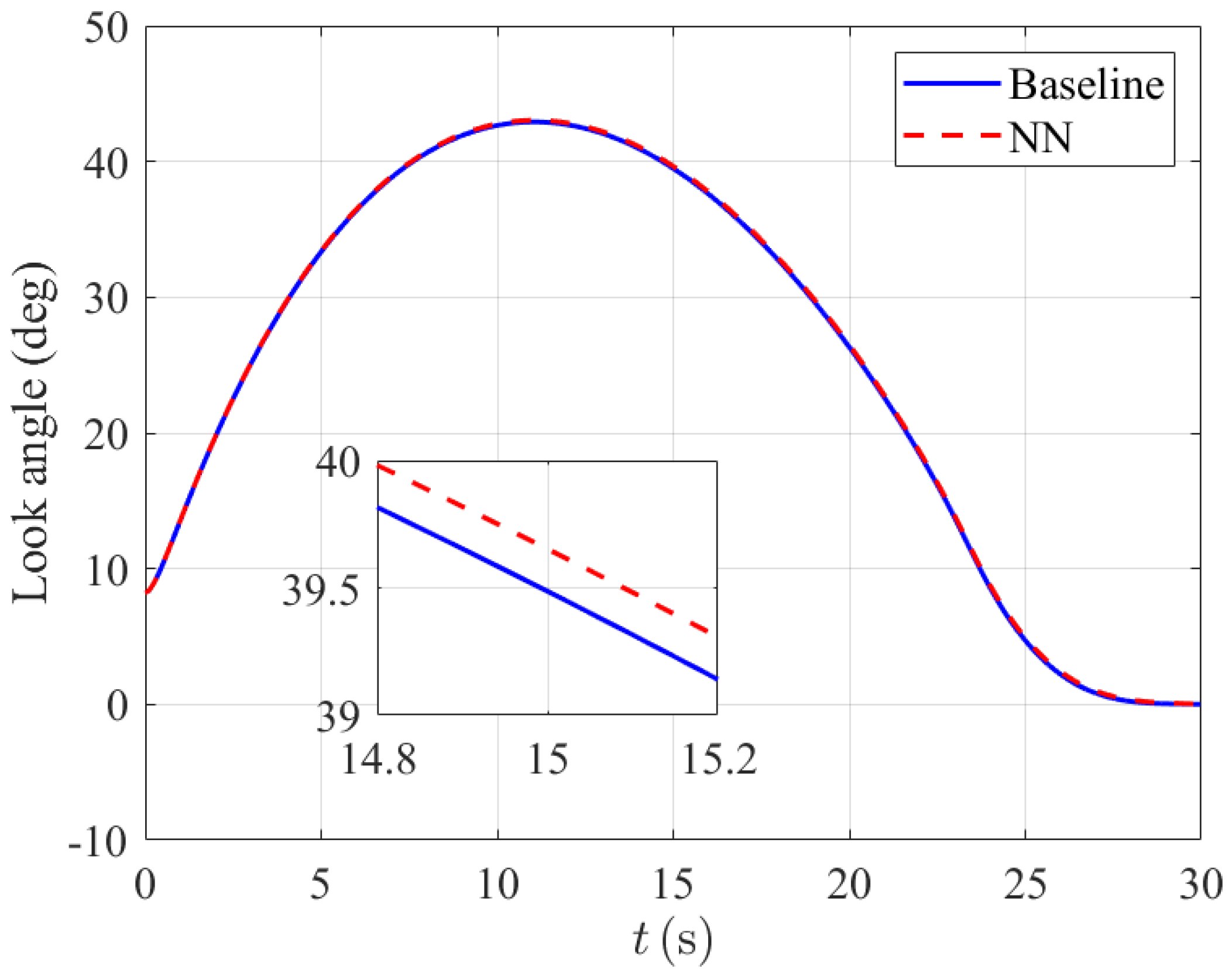
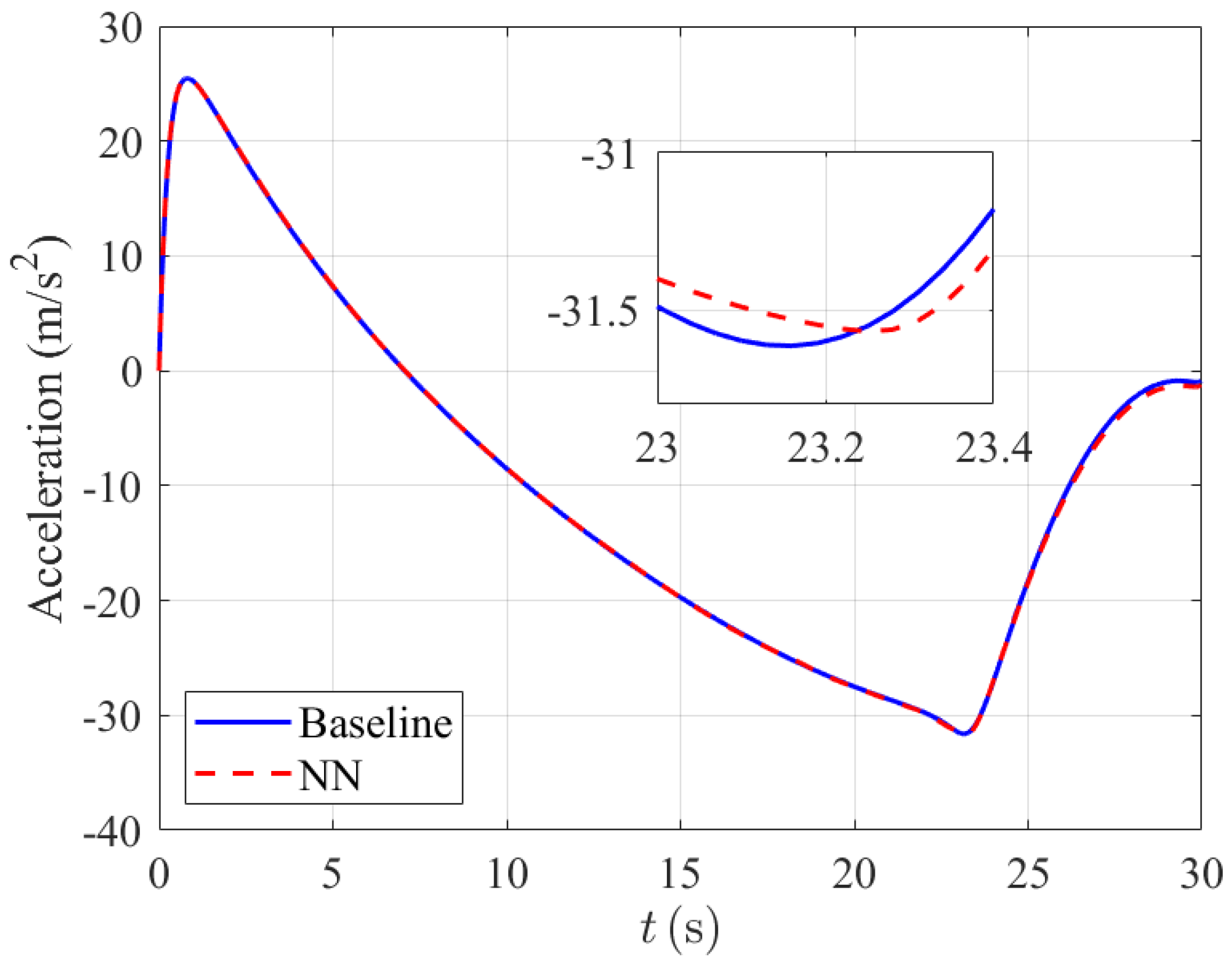
4.1. Trajectory Comparison

The purpose of the simulation studies in this section is to verify that the proposed method can indeed guide the pursuer to the target at the desired impact time, offering similar performance to the original BPN method in terms of impact time control.

We compare the pursuer under the neural network-facilitated guidance law with that under the BPN method. As the simulation results show in Figure 2, Figure 3, Figure 4 and Figure 5, the proposed approach can achieve a similar performance as the baseline method. To be more specific, the root of mean square errors (RMSEs) of downrange and crossrange trajectories of the proposed method with respect to the baseline are 1.88 m and 4.72 m, respectively. In addition, the RMSEs of range, look angle, and acceleration histories are 4.42 m, 0.14 deg, and 0.14 m/s². These verify the effectiveness of the neural network in learning from the original BPN with the competitive capability to impact on time.

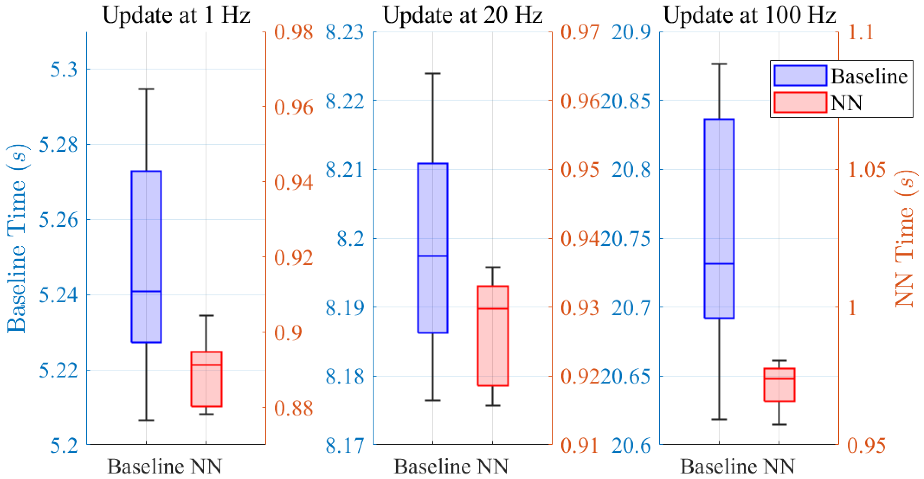
4.2. Time Consumption Comparison at Equal Update Frequency

This section shows the results of the time consumption comparison between the proposed and the original methods when operating at the same update frequency. Time consumption is calculated as the total time taken to reach the target from the starting point in the simulation environment. The update frequencies are set to be 1, 20, and 100 Hz. The engagement accuracy is also examined.

We draw the time consumption of the original and the proposed methods under different update frequencies as box plots. For each given update frequency, we conducted 10 repeated simulations. Additionally, for better visualization, in each subplot of Figure 6 with the same update frequency, we displayed the time consumption of the baseline and neural network methods near their respective means and set the same vertical axis display range to observe the variance changes. According to Figure 6 and

Table 1. Time consumption statistics at equal update frequency.

Time Cost (s)	1 Hz	20 Hz	100 Hz
Baseline method	5.25	8.20	20.75
Proposed method	0.89	0.93	0.97

, the proposed method achieves lower time consumption at every given update frequency. Moreover, the time cost variance of the proposed guidance law is also smaller and increases more slowly as the update frequency becomes higher.

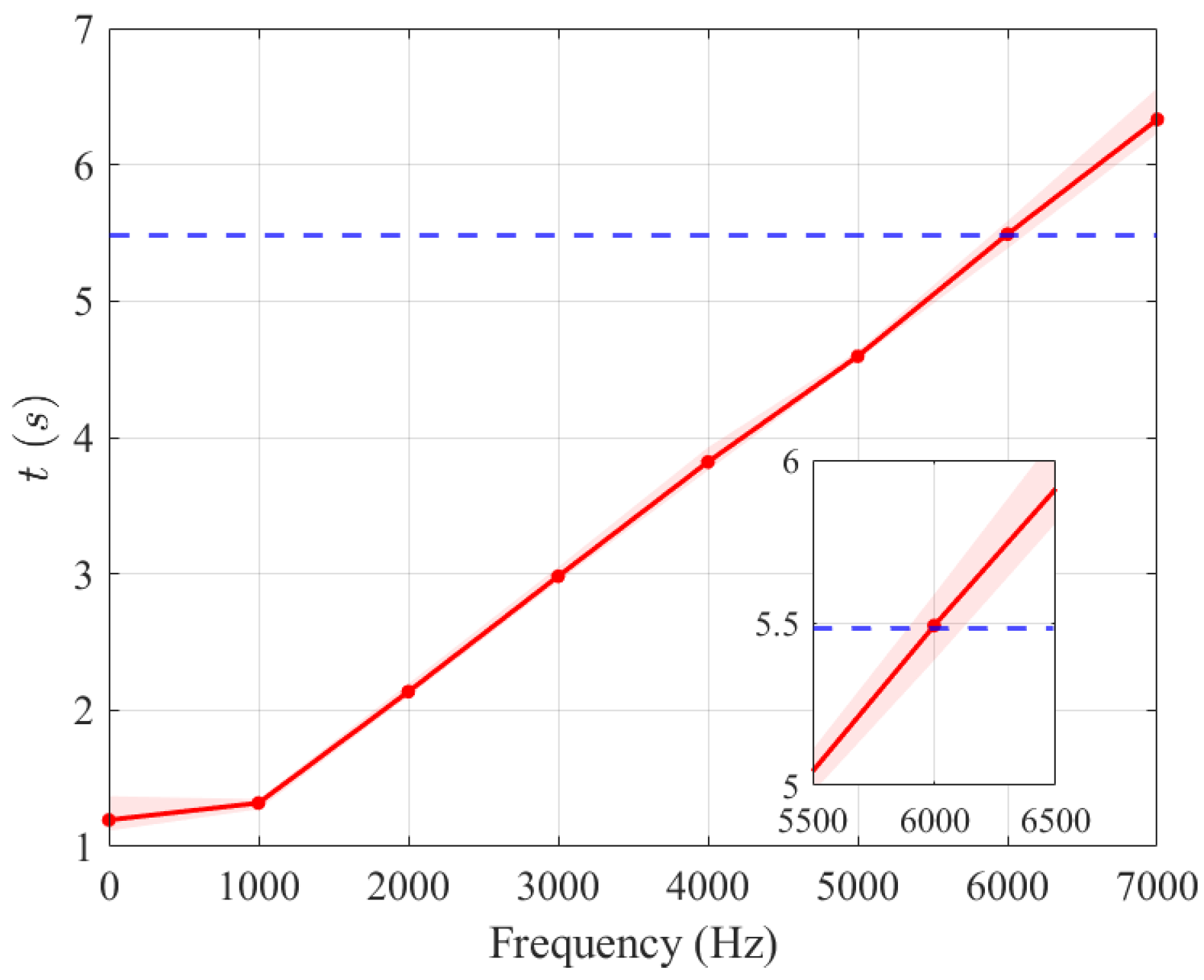
4.3. Update Frequency Comparison at Equal Real-World Time Usage

The simulation studies in this section are driven by real-world implementation concerns. The update frequency is a critical factor in the guidance system as it directly affects the actual performance of the guidance system. The update frequency is manually adjusted to the maximum value that the testing environment can handle. Considering that the computational power of the testing platform is supposedly higher than the actual hardware, the difference should be more significant in the real world.

For a more intuitive comparison, we set the update frequency of the baseline method at 1 Hz and recorded its real-time cost as 5.48 s over 10 repeated simulations in Figure 7. Then, we gradually increased the update frequency of the proposed method until its time consumption coincided with that of the baseline. As Figure 8 suggests, the proposed method can be updated at about 6000 Hz, given the time consumed by the baseline method being updated at 1 Hz, which strongly validates the higher computation efficiency of the proposed method.

5. Conclusions

This paper introduced a biased proportional navigation guidance law enhanced by a neural network. It offers a straightforward upgrade of the original approach by replacing the root-finding algorithm with a neural network. The neural network is trained using a dataset generated by the original method. The training scheme is justified. The proposed method provides similar performance but with a vast improvement in the computational efficiency. It shows how machine learning can be integrated into a traditional framework with minimum design efforts; however, a fair enhancement can be anticipated. In the future, we will explore implementing sigma-pi networks and Kolmogorov–Arnold networks to reduce parameters and further reduce the computational efficiency. Applications of the proposed method in different fields will also be investigated.

References

1. He, S.; Lee, C.H.; Shin, H.S.; Tsourdos, A. Optimal three-dimensional impact time guidance with seeker’s field-of-view constraint. Chin. J. Aeronaut. 2021, 34, 240–251. [Google Scholar] [CrossRef]
2. Chai, R.; Guo, Y.; Zuo, Z.; Chen, K.; Shin, H.S.; Tsourdos, A. Cooperative motion planning and control for aerial-ground autonomous systems: Methods and applications. Prog. Aerosp. Sci. 2024, 146, 101005. [Google Scholar] [CrossRef]
3. Narayanaswamy, S.; Damaren, C.J. Equinoctial Lyapunov control law for low-thrust rendezvous. J. Guid. Control Dyn. 2023, 46, 781–795. [Google Scholar] [CrossRef]
4. Oguri, K.; McMahon, J.W. Robust spacecraft guidance around small bodies under uncertainty: Stochastic optimal control approach. J. Guid. Control Dyn. 2021, 44, 1295–1313. [Google Scholar] [CrossRef]
5. Peterson, J.T.; Singh, S.K.; Junkins, J.L.; Taheri, E. Lyapunov guidance in orbit element space for low-thrust cislunar trajectories. In Proceedings of the AAS Guidance, Navigation and Control, Breckenridge, CO, USA, 30 January–5 February 2020; pp. 20–115. [Google Scholar]
6. Tsalik, R.; Shima, T. Circular impact-time guidance. J. Guid. Control. Dyn. 2019, 42, 1836–1847. [Google Scholar] [CrossRef]
7. Tekin, R.; Erer, K.S.; Holzapfel, F. Polynomial shaping of the look angle for impact-time control. J. Guid. Control. Dyn. 2017, 40, 2668–2673. [Google Scholar] [CrossRef]
8. Hong, H.; Tekin, R.; Holzapfel, F. Guaranteed smooth trajectory generation for field-of-view constrained impact-time control. J. Guid. Control. Dyn. 2021, 44, 898–904. [Google Scholar] [CrossRef]
9. Kim, H.G.; Lee, J.Y.; Kim, H.J.; Kwon, H.H.; Park, J.S. Look-angle-shaping guidance law for impact angle and time control with field-of-view constraint. IEEE Trans. Aerosp. Electron. Syst. 2019, 56, 1602–1612. [Google Scholar] [CrossRef]
10. Ryoo, C.K.; Cho, H.; Tahk, M.J. Time-to-go weighted optimal guidance with impact angle constraints. IEEE Trans. Control. Syst. Technol. 2006, 14, 483–492. [Google Scholar] [CrossRef]
11. Lee, C.H.; Kim, T.H.; Tahk, M.J. Effects of time-to-go errors on performance of optimal guidance laws. IEEE Trans. Aerosp. Electron. Syst. 2015, 51, 3270–3281. [Google Scholar] [CrossRef]
12. Dhananjay, N.; Ghose, D. Accurate time-to-go estimation for proportional navigation guidance. J. Guid. Control. Dyn. 2014, 37, 1378–1383. [Google Scholar] [CrossRef]
13. Tahk, M.J.; Shim, S.W.; Hong, S.M.; Choi, H.L.; Lee, C.H. Impact time control based on time-to-go prediction for sea-skimming antiship missiles. IEEE Trans. Aerosp. Electron. Syst. 2018, 54, 2043–2052. [Google Scholar] [CrossRef]
14. Jeon, I.S.; Lee, J.I.; Tahk, M.J. Impact-time-control guidance with generalized proportional navigation based on nonlinear formulation. J. Guid. Control Dyn. 2016, 39, 1885–1890. [Google Scholar] [CrossRef]
15. Dong, W.; Wang, C.; Wang, J.; Xin, M. Varying-gain proportional navigation guidance for precise impact time control. J. Guid. Control Dyn. 2023, 46, 535–552. [Google Scholar] [CrossRef]
16. Jiang, Z.; Ge, J.; Xu, Q.; Yang, T. Impact time control cooperative guidance law design based on modified proportional navigation. Aerospace 2021, 8, 231. [Google Scholar] [CrossRef]
17. Saleem, A.; Ratnoo, A. Two stage proportional navigation guidance law for impact time control. In Proceedings of the 2018 Indian Control Conference (ICC), Kanpur, India, 4–6 January 2018; IEEE: Piscataway, NJ, USA, 2018; pp. 312–317. [Google Scholar]
18. Kumar, S.R.; Mukherjee, D. True-proportional-navigation inspired finite-time homing guidance for time constrained interception. Aerosp. Sci. Technol. 2022, 123, 107499. [Google Scholar] [CrossRef]
19. Jeon, I.S.; Lee, J.I.; Tahk, M.J. Impact-time-control guidance law for anti-ship missiles. IEEE Trans. Control Syst. Technol. 2006, 14, 260–266. [Google Scholar] [CrossRef]
20. Erer, K.S.; Tekin, R.; Hong, H. Computational Impact-Time Guidance with Biased Proportional Navigation. J. Guid. Control Dyn. 2024, 47, 1–7. [Google Scholar] [CrossRef]
21. Jin, T.; He, S. Ensemble Transfer Learning Midcourse Guidance Algorithm for Velocity Maximization. J. Aerosp. Inf. Syst. 2023, 20, 204–215. [Google Scholar] [CrossRef]
22. Liu, Z.; Wang, J.; He, S.; Shin, H.S.; Tsourdos, A. Learning prediction-correction guidance for impact time control. Aerosp. Sci. Technol. 2021, 119, 107187. [Google Scholar] [CrossRef]
23. Izzo, D.; Öztürk, E. Real-time guidance for low-thrust transfers using deep neural networks. J. Guid. Control Dyn. 2021, 44, 315–327. [Google Scholar] [CrossRef]
24. Singh, S.K.; Junkins, J.L. Stochastic learning and extremal-field map based autonomous guidance of low-thrust spacecraft. Sci. Rep. 2022, 12, 17774. [Google Scholar] [CrossRef] [PubMed]
25. Izzo, D.; Blazquez, E.; Ferede, R.; Origer, S.; De Wagter, C.; de Croon, G.C. Optimality principles in spacecraft neural guidance and control. Sci. Robot. 2024, 9, eadi6421. [Google Scholar] [CrossRef] [PubMed]
26. He, S.; Shin, H.S.; Tsourdos, A. Computational missile guidance: A deep reinforcement learning approach. J. Aerosp. Inf. Syst. 2021, 18, 571–582. [Google Scholar] [CrossRef]
27. Siddique, U.; Sinha, A.; Cao, Y. On Deep Reinforcement Learning for Target Capture Autonomous Guidance. In Proceedings of the AIAA SCITECH 2024 Forum, Orlando, FL, USA, 8–12 January 2024; p. 0957. [Google Scholar]
28. Sinha, A.; White, D.; Cao, Y. Deep Reinforcement Learning-based Optimal Time-constrained Intercept Guidance. In Proceedings of the AIAA SCITECH 2024 Forum, Orlando, FL, USA, 8–12 January 2024; p. 2206. [Google Scholar]
29. Erer, K.S.; Merttopçuoglu, O. Indirect impact-angle-control against stationary targets using biased pure proportional navigation. J. Guid. Control Dyn. 2012, 35, 700–704. [Google Scholar] [CrossRef]
Figure 1. Engagement geometry.
Aerospace 11 00670 g001
Figure 2. Trajectories of baseline and proposed methods.
Aerospace 11 00670 g002
Figure 3. Range histories of baseline and proposed methods.
Aerospace 11 00670 g003
Figure 4. Look angle histories of baseline and proposed methods.
Aerospace 11 00670 g004
Figure 5. Acceleration histories of baseline and proposed methods.
Aerospace 11 00670 g005
Figure 6. Time cost comparison at equal update frequencies.
Aerospace 11 00670 g006
Figure 7. Time cost at 1 Hz of baseline method.
Aerospace 11 00670 g007
Figure 8. Time cost of proposed method regarding increasing update frequency.
Aerospace 11 00670 g008