Article

Adaptive Incremental Nonlinear Dynamic Inversion Control for Aerial Manipulators

Department of Mechanical Engineering, University of Calgary, Calgary, AB T2N 1N4, Canada
*
Author to whom correspondence should be addressed.
Aerospace 2024, 11(8), 671; https://doi.org/10.3390/aerospace11080671
Submission received: 29 June 2024 / Revised: 4 August 2024 / Accepted: 12 August 2024 / Published: 15 August 2024
(This article belongs to the Special Issue Challenges and Innovations in Aircraft Flight Control)

Abstract

:
This paper proposes an adaptive incremental nonlinear dynamic inversion (INDI) controller for unmanned aerial manipulators (UAMs). A novel adaptive law is employed to enable aerial manipulators to manage the inertia parameter changes that occur when the manipulator moves or picks up unknown objects during any phase of the UAM’s flight maneuver. The adaptive law utilizes a Kalman filter to estimate a set of weighting factors employed to adjust the control gain matrix of a previously developed INDI control law formulated for the corresponding UAV (no manipulator included). The proposed adaptive control scheme uses acceleration and actuator input measurements of the UAV without necessitating any knowledge about the manipulator, its movements, or the objects being grasped, thus enabling the use of previously developed INDI UAV controllers for UAMs. The algorithm is validated through simulations demonstrating that the adaptive control gain matrix used in the UAV’s INDI controller is promptly updated based on the UAM maneuvers, resulting in effective UAV and robot arm control.

1. Introduction

Unmanned aerial vehicles (UAVs) have attracted increasing attention for both military and civil operations in recent decades. Military missions, including surveillance and reconnaissance, have been successfully carried out by automated UAVs [1]. UAVs have also found applications in civil operations, such as aerial photography, providing wireless coverage, and infrastructure inspection [2]. However, current UAV missions remain limited to passive operations, where UAVs observe, collect data, or perform tasks without direct engagement or interaction with the environment or targets.
In an effort to broaden the capabilities and versatility of UAV missions, researchers have explored the integration of robotic manipulators into UAVs. The combination of UAVs with robotic manipulators is often referred to as unmanned aerial manipulators (UAMs). The addition of one or more robot arms enables UAVs to perform active operations herein defined as operations where UAVs interact and manipulate with the environment/objects. For example, UAMs could clear paths inside collapsed buildings by removing obstacles hindering navigation and perform repairs in inaccessible industrial structures, such as pipeline labyrinths and underground facilities. Despite the potential capabilities of UAMs, these capabilities are still limited, and advanced developments in control, estimation, and motion planning are required before UAMs can fully maximize their potential. An aspect of particular interest to be resolved is the ability to manage changes to the UAM’s inertia parameters, including mass, the position of the aircraft’s center of mass, and the moment of inertia tensor that occur when the arm is moved. This becomes particularly difficult when the UAM picks up an unknown mass, making it challenging to model these inertia changes accurately. This is of special interest when the aircraft and the arm move simultaneously, which is currently challenging, thus limiting the use of the arm comprising a given UAM to only move when the aircraft is in hover. In full flight, the UAM’s inertia changes can significantly impact aircraft operation and its control performance.
To address the challenge of varying inertia parameters in aircraft, various control techniques have been applied. Jimenez-Cano et al. [3] proposed a variable parameter integral backstepping controller for UAM attitude control, accounting for changes in inertia parameters and torques due to manipulator movements. Orsag et al. [4] designed UAM PID controllers and analyzed their stability under a changing moment of inertia tensor [5,6]. PID controllers, however, have shown to exhibit oscillatory behavior during grasping flight maneuvers and lead to the development of hybrid adaptive controllers [7]. There have been many other research studies that use adaptive laws to address inertia changes in aircraft [8,9,10]. Nicol et al. introduced a neural-network-based adaptive law capable of handling disturbances caused by the presence of unknown payloads and strong wind [11]. Others have estimated inertia parameters of UAVs through the use of Lyapunov functions for added payloads [12], moment of inertia changes [13], and object pick-up maneuvers [14]. For the estimation of inertia parameters, researchers [12,13,14] have employed gradient descent adaptive laws, adaptive backstepping controllers, and model reference adaptive laws. However, flight performance tends to degrade before the estimation variables converge to their true values, which require several seconds when the above-mentioned tools are used. To reduce such time dependencies, Lee and Kim proposed an online parameter estimator for unknown picked-up payloads conforming to a given Lyapunov candidate function for control purposes [15,16]. Additionally, Park et al. proposed the use of a Kalman filter, which accounts for the manipulator’s movement, to promptly estimate the inertia parameters of UAMs during manipulation maneuvers [17].
Despite these and other control efforts developed to manage varying inertia parameters, UAMs have not yet reached the desired level of performance due to the complexities associated with the highly coupled dynamics between the UAV and the manipulator. Incremental nonlinear dynamic inversion (INDI) controllers have been developed to address this challenge by increasing robustness to model uncertainties and effectively managing coupled system dynamics, which other controllers struggle to handle [18,19,20]. Due to such capabilities, INDI control schemes have been employed in UAVs, including aggressive flight control [21,22,23] and disturbance rejection [24].
While INDI demonstrates robustness and agile control performance with minimal dynamic modeling information, it faces two primary challenges. First, it requires somewhat accurate information about the vehicle’s inertia parameters, including total mass, moment of inertia tensor, and the location of the center of mass, to formulate the corresponding control effectiveness matrix that generates control input increments based on sensor measurements of the UAV. Efforts have been made to address this challenge. In [25], Smeur et al. used a least mean squares algorithm to estimate the control effectiveness matrix in real time. Cao et al. [26] combined a neural network adaptive law and an INDI controller to handle the nonlinear characteristics of fixed-wing UAVs that cannot be accounted for in the control effectiveness matrix. However, these developments have only considered time-invariant systems and have not addressed systems where the dynamics change over time. In an attempt to resolve such challenges and generate robust control effective matrices, Ahmadi et al. [27] proposed a reference model adaptive INDI controller capable of handling unmodeled dynamics from actuator faults, demonstrating that quadcopter drones can be controlled under the presence of partial actuator faults. The second issue with INDI involves ensuring that the control effectiveness matrix for the system of interest is non-singular (invertible). Although such aspects have been considered for time-invariant systems (e.g., [28,29]), challenges remain for time-variant systems, including UAMs. Thus, when controlling UAMs, it is necessary to consider the conditions that lead to singularity in the control effectiveness matrix needed to develop suitable solutions during the flight maneuvers of UAMs.
This paper presents an adaptive INDI control scheme for UAM systems that experience changes in inertia parameters that occur during the manipulator’s movements and object grasping actions while either the UAV is in hover or performing a flight maneuver. The adaptive law estimates a set of weighting factors to adapt the terms comprising the inverse of the control effectiveness matrix at each time step of the flight control process. The proposed approach captures inertia changes due to manipulation maneuvers through an adaptive process and resolves matrix singularity problems by eliminating the need for matrix inversion, resulting in effective UAM control under varying flight grasping maneuvers. The proposed formulation does not require any information about the manipulator connected to the UAV and relies solely on sensor measurements. UAVs will frequently employ different manipulators based on mission requirements, necessitating on-the-spot decisions. These manipulators can also undergo geometric or inertial changes, such as component replacement or installation, making it impractical and costly to measure their parameters each time. Therefore, the proposed algorithm offers significant benefits under these circumstances.
The remainder of this paper is structured as follows. Section 2 provides an overview of the UAM system and its dynamic model used in this research. Section 3 describes the INDI control scheme that is employed in this paper for UAMs formulated based on previous work on highly maneuverable UAVs [28,29]. Section 4 describes the proposed adaptive INDI control scheme. Section 5 provides simulation results, and Section 6 concludes the paper with general observations and future work.

2. UAM Dynamic System Model

In this research, a highly maneuverable tilt rotorcraft VTOL vehicle named Navig8 (Figure 1a) with a three-degree-of-freedom (DoF) manipulator (Figure 1b) is used as the targeted dynamic system platform.

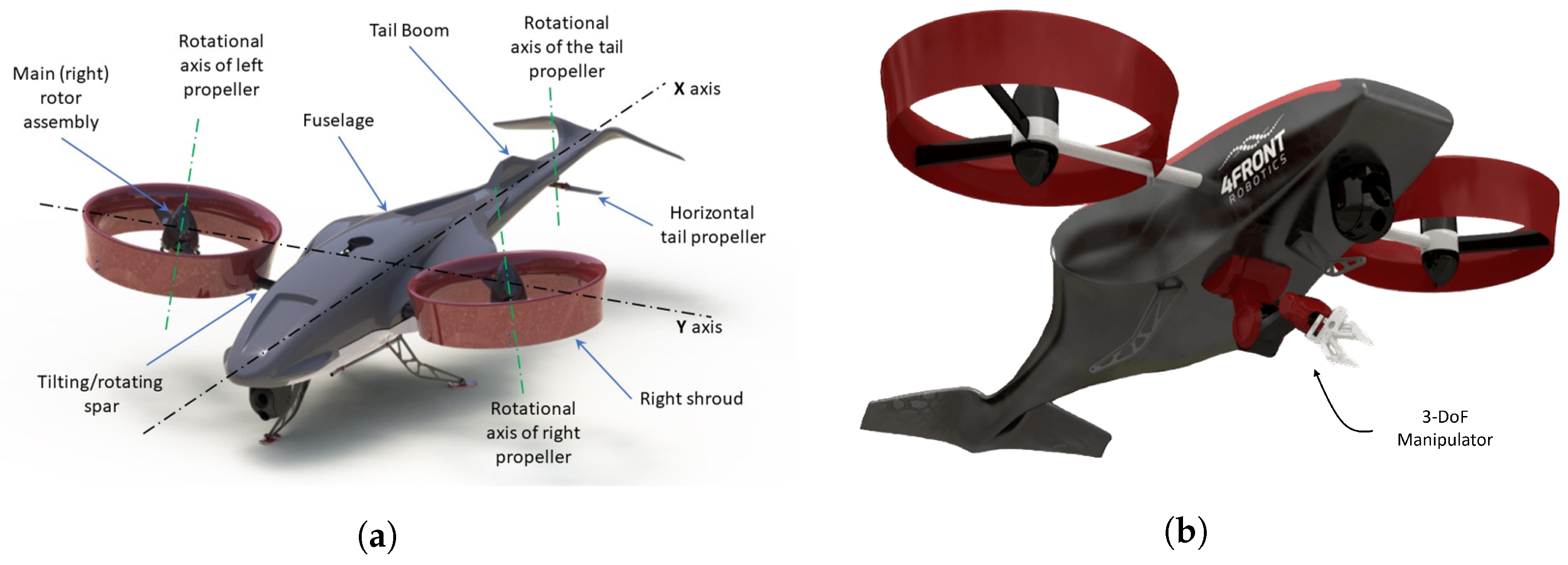
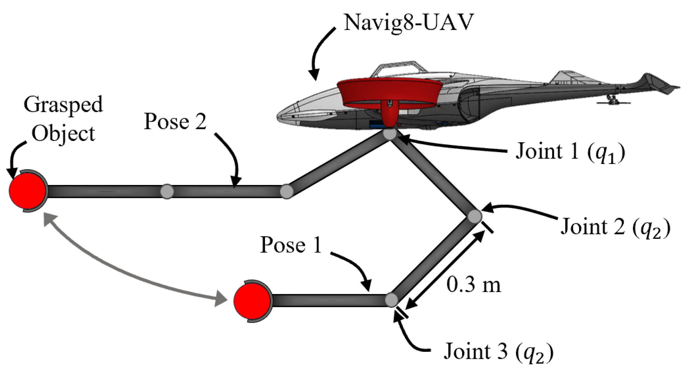
2.1. Navig8-UAM System

The Navig8-UAV, developed primarily for operations inside confined spaces, is a scalable tilt-rotorcraft with two (left and right) ducted variable-pitch (VP) propellers and one horizontal VP (non-tiltable) tail propeller (Figure 1a). To reduce aerodynamic ground and wall effects, the two main propellers include a dihedral angle, γ , and are shrouded to increase thrust. This configuration enables the UAV to execute unconventional aerobatic maneuvers at slow speeds, suitable for flight inside confined spaces, including hovering in any non-zero pitch attitude. Such capabilities facilitate take-off and landing on inclined surfaces (e.g., mountains) and perching on vertical walls and ceilings. Various control methods have been previously developed for both the Navig8-UAV [30,31,32] and the Navig8-UAM [33]. Notably, a novel INDI2 + PD control architecture for the Navig8-UAV has been developed, demonstrating satisfactory control performance [28,29]. The control efforts for the Navig8-UAM have been limited to include 2 DoF simple low-weight robot arms, where the effect of inertia parameters is minimal [33]. In this paper, the previously mentioned control architectures are extended to manage UAMs, where the UAM’s inertia changes due to the arm motions/tasks have a profound effect on the system, marking the first instance of such an extension. The modeling approach for Navig8-UAM in this paper differs from the method presented in [33]. This paper considers the UAM as a unified system, whereas [33] treats the UAV and the robot arm as distinct entities.
The Navig8-UAM, depicted in Figure 1b, incorporates a 3 DoF manipulator attached to the UAV’s underside, where the rotational axes of its joints are parallel to one another, thereby constraining the manipulator’s motion to the longitudinal plane of the UAV ( x ^ z ^ plane) as illustrated in Figure 2. The arm includes an end-effector capable of grasping objects of diverse size and weight. The Navig8-UAM is symmetric with respect to the longitudinal plane of the UAV.
It is essential to note that the addition of the manipulator to the UAV results in dynamic changes in the center of mass from the UAV ( C o M U A V ) to the UAM ( C o M U A M ), denoted as the position vector r o f f in Figure 2. This displacement varies as the manipulator moves and/or interacts with objects. As a result, the dynamic equations reported in [28,29] are enhanced to consider the UAM.

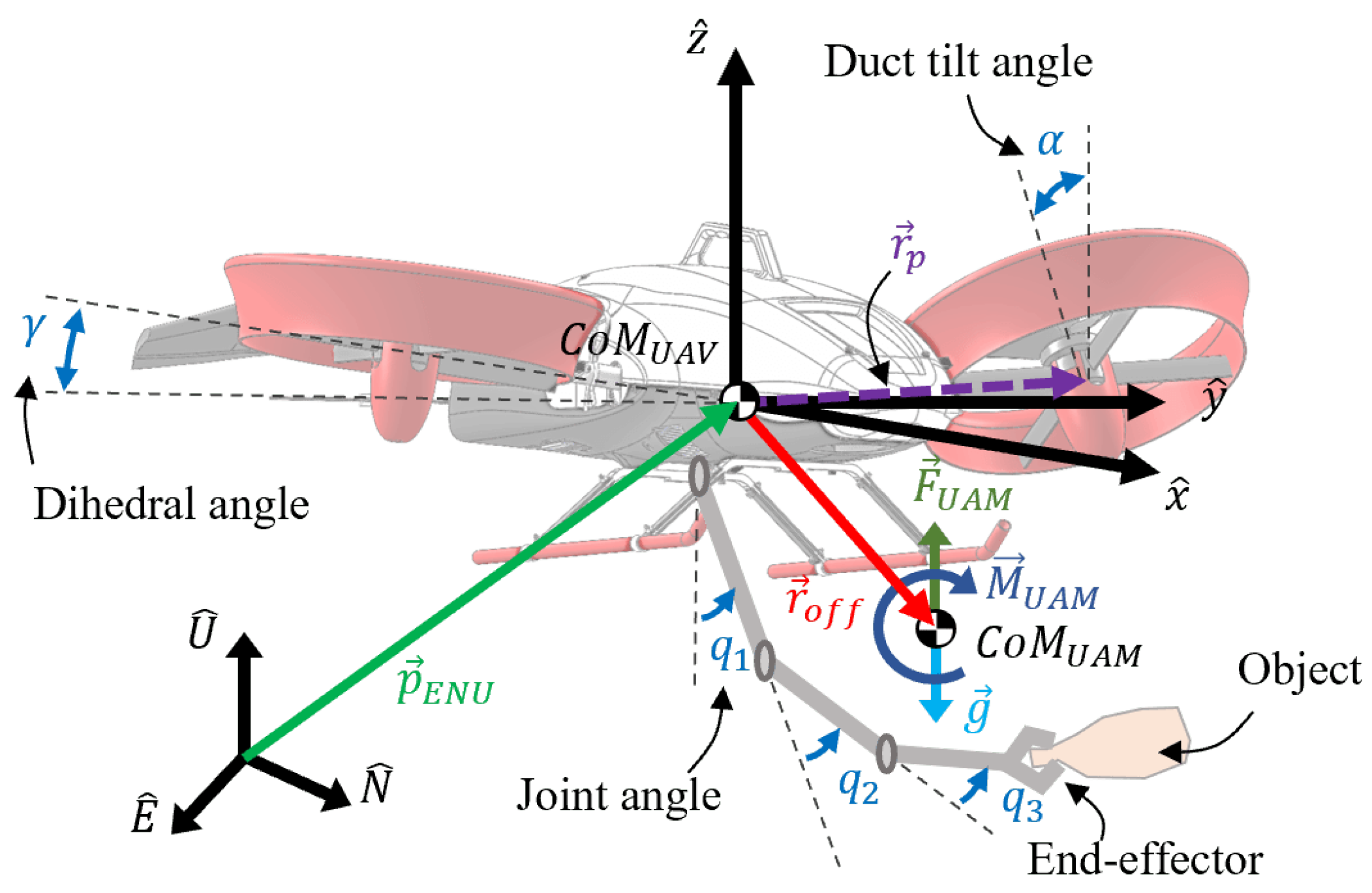
2.2. Force and Moment Equations for the Navig8-UAM
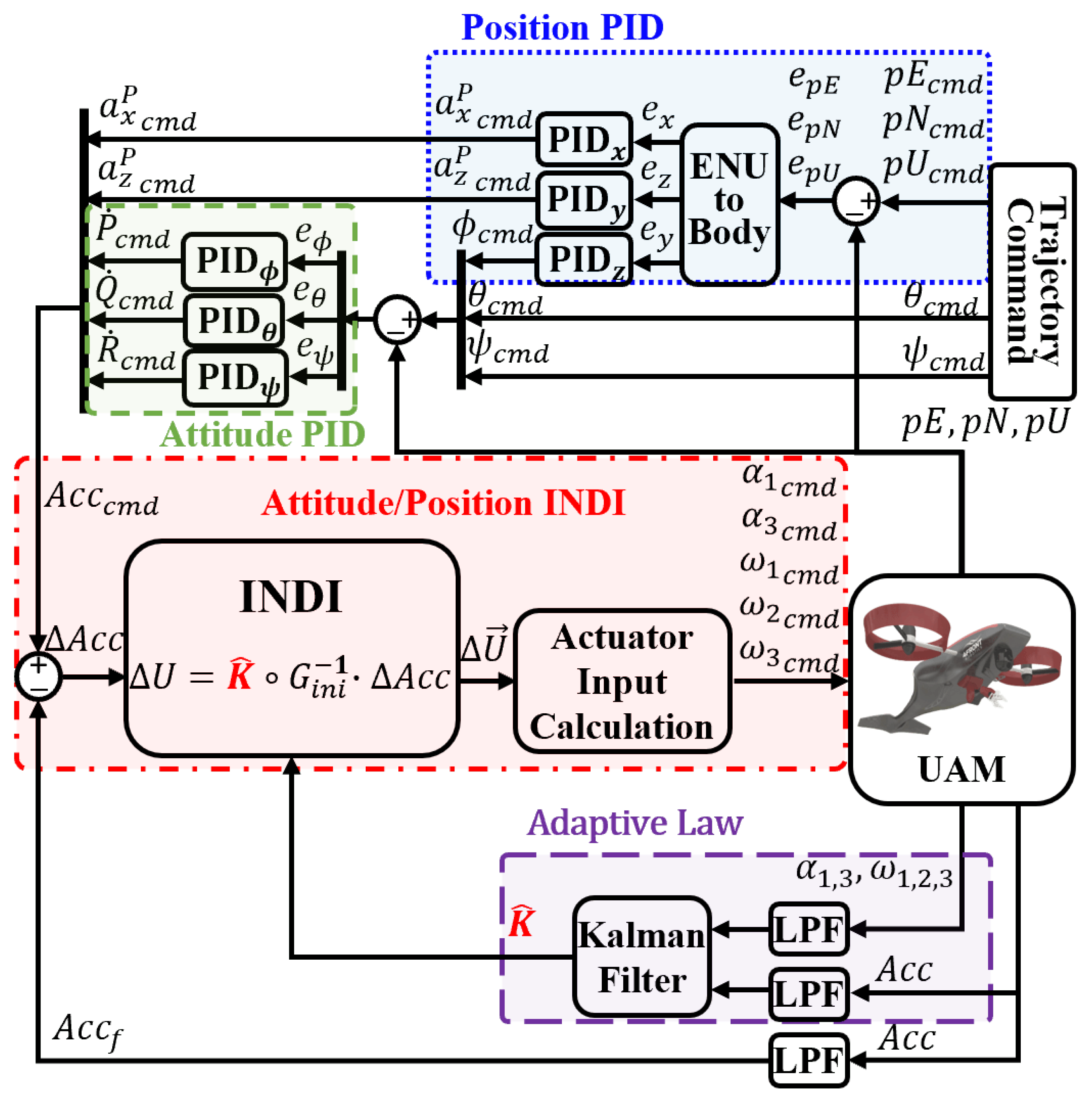
The force and moment equations of motion for the Navig8-UAM are derived from Newton’s second law with respect to the UAV frame of reference. This frame of reference is used because it remains fixed at the UAV’s center of mass (Figure 2) and is unaffected by the movement of the arm, whereas the UAM frame of reference at the UAM’s center of mass varies with manipulation maneuvers. The developed equations are extensions of the mathematical model described in [28,29]. The force equation around the UAM is expressed with respect to the UAV frame of reference as Equation (1):
F U A M = m U A M a U A M P
where F U A M represents the total force acting on the UAM, excluding the gravitational force, m U A M denotes the total mass of the UAM (UAV + arm), including the mass of objects held by the manipulator, and a U A M P represents the UAM’s linear acceleration without the gravitational acceleration (i.e., a U A M P = a U A M g ). Notably, the linear acceleration of the UAM is distinguished from the linear acceleration of the UAV ( a U A V p ) as movements of the arm or rotation of the UAM introduce additional linear acceleration to the UAV. The relationship between a U A M P and a U A V P is expressed by Equation (2):
a U A M P = a U A V P + a a d d
where a a d d = d 2 d t 2 r o f f + α U A V × r o f f + 2 ω U A V × d d t r o f f + ω U A V × ω U A V × r o f f , ω U A V = P , Q , R T , and α U A V = P ˙ , Q ˙ , R ˙ T are the angular velocity and acceleration of the UAV, respectively (i.e., P, Q, and R represent the rotational speeds of the UAV in the x ^ , y ^ , and z ^ directions of the UAV reference frame). Additionally, r o f f is a displacement vector from the UAV’s center of mass to the UAM’s center of mass (Figure 2).
The moment equation of the UAM is described with respect to the UAV frame of reference by Equation (3):
M U A M = I U A M · α U A M + ω U A M × I U A M · ω U A M
where I U A M represents the moment of inertia tensor of the UAM in the UAV reference frame. Similarly to the linear acceleration, the angular velocity and acceleration of the UAM, represented as ω U A M and α U A M , are distinguished from those of the UAV, denoted as ω U A V and α U A V . This representation is necessary to identify the variations that the manipulator’s movements induce to the UAV. Thus, the mathematical equation for the angular velocity and angular acceleration between the UAM and UAV is described by Equations (4) and (5), respectively:
ω U A M = ω U A V ω i n t
α U A M = α U A V α i n t ω U A V × ω i n t
where ω i n t and α i n t denote the relative (internal) angular velocity and acceleration of the UAV with respect to the UAM.
The knowledge regarding the manipulator movements, including its joint angles q, velocities q ˙ , and acceleration q ¨ , as well as inertia information (mass and moment of inertia tensor), is captured by Equations (2), (4) and (5) via terms such as r o f f , ω i n t , α i n t , m U A M , and I U A M .
In this research work, the UAM’s motion is considered to be executed under slow-speed conditions in calm air, where aerodynamic forces and torques (e.g., drag) can be neglected. Thus, it is assumed that the sole forces and torques acting on the UAM are those resulting from the propellers’ movements (rotation and tilt) as Equations (6) and (7):
F U A M = F p 1 + F p 2 + F p 3
M U A M = r p 1 × F p 1 + r p 2 × F p 2 + r p 3 × F p 3 r o f f × ( F p 1 + F p 2 + F p 3 ) + Q p 1 + Q p 2 + Q p 3
where F p i and Q p i denote the propeller force and torque generated by the ith propeller, and r p i represents the position vector from the center of mass of the UAV to the ith propeller (Figure 2). The fourth term ( r o f f × ( F p 1 + F p 2 + F p 3 ) ) in Equation (7) arises from the displacement of the center of mass due to the combination of the manipulator.
The motion of the robotic arm affects the motion of the UAV through the reaction force and torque that are produced on the aircraft. These forces and torques, however, can be considered as internal forces and torques within the UAM system; thus, they do not influence the motion of the UAM, in accordance with the conservation of momentum.
In a similar fashion as carried out in [28,29], for the purpose of controller design, the control input vector, U, is formulated as a combination of actuator inputs, which include the propellers’ rotational speeds (i.e., ω p i for i = 1 to 3 ), and the tilt angles of the two main shrouded propellers (i.e., α 1 and α 3 ) as represented in Equation (8):
U = u 1 u 2 u 3 u 4 u 5 T = cos α 1 ω p 1 2 sin α 1 ω p 1 2 cos α 3 ω p 3 2 sin α 3 ω p 3 2 ω p 2 2 T
Thus, the control input vector, U, provides corresponding actuator inputs to be sent to the UAV, as described in Equation (9):
ω p 1 ω p 2 ω p 3 α 1 α 3 = u 1 2 + u 2 2 4 u 5 u 3 2 + u 4 2 4 arctan u 2 u 1 arctan u 4 u 3

3. INDI for UAMs

An effective INDI control architecture for the Navig8-UAV (without a manipulator), referred as the INDI2 + PD, has been developed and described in [28,29]. In this section, the INDI2 + PD controller is adapted and used for developing the proposed adaptive INDI control law for the Navig8-UAM. The INDI2 + PD controller is a cascade control architecture composed of an attitude and a position INDI controller. Herein, the INDI control is derived following the same procedure as in [28,29]. However, this derivation uses the force and moment equations of the UAM, which include the manipulator.

3.1. Rotational Relationship

The INDI controller responsible for rotational motions is devised by reformulating the moment equation (Equation (3)) in terms of the UAV’s angular acceleration as shown in Equation (10):
α U A V = I U A M 1 M U A M α a d d
where α a d d = α i n t ω U A V × ω i n t + I U A M 1 ω U A V + ω i n t × I U A M · ω U A V ω i n t . Equation (10) is linearly approximated using the first-order Taylor expansion, which leads to Equation (11):
α U A V I U A M 0 1 M U A M 0 α a d d 0 + X I U A M 1 M U A M α a d d · X X 0 + U I U A M 1 M U A M α a d d · U U 0
The terms within the first set of parentheses in Equation (11) represent the components at the linearized point, which corresponds to the current time denoted by the subscript “0”. Thus, such components denote the measured angular acceleration of the UAV, α U A V 0 , at the current time. The terms within the second set of parentheses represent the contribution arising from the change in the UAV state vector, X, comprising 12 terms defined as per Equation (12):
X = [ p E p N p U ϕ θ ψ p E ˙ p N ˙ p U ˙ P Q R ] T
where ( p E , p N , p U ) denotes the UAV’s position in the inertial frame of reference, ( ϕ , θ , ψ ) represents the UAV’s roll, pitch, and yaw angles, and (P, Q, R) represents the angular velocity of the UAV. Assuming that the response of the UAV’s actuators (motors for propeller rotation and servo motors for shroud tilting) is significantly faster than the change in the UAV state, and that the sensor’s sampling time is sufficiently fast, it can be said that the change in the UAV state, ( X X 0 ), is negligible compared to the control input changes, ( U U 0 ), leading to X X 0 . This assumption is frequently used in the INDI controller design procedure [22,23,24,25,26,27,28,34] and is often referred to as the principle of time scale separation [20]. Thus, the second part of Equation (11) is considered negligible and removed from the control signal computation. Therefore, Equation (11) can be simplified to Equation (13):
α U A V = α U A V 0 + I U A M 1 M U A M U · U U 0
Equation (13) thus represents the rotational relationship between control inputs and angular accelerations, which will be used to formulate the INDI controller.

3.2. Translational Relationship

In a similar fashion, the force equation (Equation (1)) can be reformulated in terms of the linear acceleration of the UAV, resulting in Equation (14):
a U A V = F U A M m U A M a a d d
Through the application of the Taylor expansion, Equation (14) is linearized, yielding Equation (15):
a U A V F U A M 0 m U A M 0 a a d d 0 + X F U A M m U A M a a d d · X X 0 + U F U A M m U A M a a d d · U U 0
Similar to Equation (11), the first part of Equation (15) corresponds to the current linear acceleration of the UAV, a U A V 0 , which is measured via the UAV’s on-board sensors (i.e., IMU). Under the similar conditions used in Section 3.1 (e.g., swift actuator dynamics and a sensor high sampling rate) the change in UAV state is considered to be zero (i.e., X X 0 = 0 ). As a result, after computing the partial derivatives, Equation (15) simplifies to Equation (16):
a U A V = a U A V 0 + 1 m U A M F U A M U · U U 0

3.3. INDI Formulation

From Equation (13) in Section 3.1 and the x and z components of Equation (16) in Section 3.2, the relationship between the acceleration increments, Δ A c c =   [ α U A V α U A V 0 ;   a U A V x , z a U A V 0 x , z ] , and the control input increments, Δ U = U U 0 = [ Δ u 1 , Δ u 2 , Δ u 3 , Δ u 4 , Δ u 5 ] T , is formulated as per Equations (17) and (18):
Δ A c c = I U A M 1 M U A M U 1 m U A M F U A M x , z U · Δ U = G · Δ U
Δ U = G 1 · Δ A c c
It is worth noting that the y component of Equation (16) is not used because the vehicle is underactuated in terms of the linear acceleration in the y direction. By inverting the 5 × 5 matrix G in Equation (17) and multiplying it by the desired acceleration increments, the necessary control input increments can be computed as shown in Equation (18). The complete control input vectors are formulated as shown in Equation (19):
U = U 0 + Δ U
The actuator inputs can then be obtained by using Equation (9). The details of matrix G for the Navig8-UAM are presented in Appendix A.

3.4. Control Effectiveness Matrix

The matrix G in Equation (17) is often referred to as the control effectiveness matrix. The control effectiveness matrix G plays a crucial role in determining the control performance of INDI controllers. It produces the necessary control input increments to achieve the desired acceleration increments. While the matrix G can be analytically obtained by applying the Taylor expansion to the system’s moment and force equations, its components are dependent on the inertia parameters of the UAM. As the manipulator moves and picks up unknown masses, such parameters (i.e., total mass, moment of inertia tensor, and the center of mass position of the UAM) constantly change, making it difficult to model. This dynamic nature makes it challenging to establish a single fixed control effectiveness matrix for all flight grasping and arm movement scenarios, unless the inertia information of the UAM, including the object, does not change or is provided at every corresponding specific moment in time. Therefore, there is a need to adapt the G matrix according to the current inertia state of the UAM. When adapting the control effectiveness matrix to the current flight state, or, generally, when the system’s inertia parameters/configurations change as UAM scenarios, it is crucial to ensure that the matrix G remains invertible at all times during the flight mission (so that Equation (18) can be used). The conditions under which G becomes singular as the UAM moves need to be identified in real time or computed analytically and avoided for all flight and robot arm movement states. However, in this paper, this necessity is removed. The following section describes the adaptive INDI control architecture capable of computing a set of weighting values used to update the theoretical G 1 matrix of the Navig8-UAV in real time. The proposed approach enables the control architecture developed for the UAV to be capable of controlling the UAM version of the UAV without prior knowledge of the robot’s arm, its motion, or the object being grasped. The methodology enables the UAM to effectively compute the corresponding control signals to maneuver the UAM as desired despite the inertia changes in the system due to the manipulator maneuvers. This is achieved via an adaptive estimation process.

4. Adaptive INDI for UAMs

The challenges mentioned in Section 3.4 are resolved by directly adapting the inverse of matrix G in this paper. This section outlines the adaptive mechanism for computing G 1 as the UAV flies while the arm is simultaneously used.

4.1. Methodology

As per Equation (17), the control effective matrix G (as well as its inverse, G 1 ) represents the relationship between the changes in control inputs and the resulting acceleration changes of the UAV within the UAM system. This implies that G 1 can be estimated based on the knowledge about the current control inputs (or actuator inputs) and the corresponding resulting acceleration achieved by the UAV, which can be measured. To achieve this, a previously developed INDI controller [28,29] for the aircraft of interest is extended, resulting in the adaptive INDI control architecture.
Figure 3 illustrates the proposed extended INDI control structure for the UAM, which we refer to as the adaptive INDI controller.
As reported in [29], the controller operates on a trajectory that the UAV is required to track. Trajectory commands for the UAV include the desired position ( p E c m d , p N c m d , p U c m d ) in the inertial frame of reference and the desired pitch and yaw attitude ( θ c m d , ψ c m d ) of the UAV. As represented by the blue box with a dotted outline in Figure 3, the adapted control algorithm begins by computing the inertial position error of the UAV ( e p E , e p N , e p U ) by subtracting the current UAV’s inertial position from the desired inertial position. Then, the reference frame of the position error is transformed to the UAV’s body frame ( e x , e y , e z ). These position errors in the UAV’s reference frame are employed by a set of three PID controllers to generate the desired linear acceleration in the x and z directions ( a x c m d P , a z c m d P ), along with the required roll attitude ( ϕ c m d ). Notably, for the desired lateral translation, the desired roll attitude is generated rather than directly generating the y-directional linear acceleration due to the UAV’s underactuated characteristics in the y-direction. This desired roll attitude, along with the desired pitch and yaw attitude obtained from the given UAV trajectory, are employed by a second set of three PID controllers as represented in the green box in Figure 3. These attitude PID controllers produce the corresponding desired angular acceleration of the UAV in the x, y, and z directions ( P ˙ c m d , Q ˙ c m d , R ˙ c m d ). The desired linear acceleration in the x and z directions ( a x c m d P , a z c m d P ) and the desired angular acceleration of the UAV ( P ˙ c m d , Q ˙ c m d , R ˙ c m d ), collectively denoted as A c c c m d , are used as the inputs to the attitude and position INDI controller, as detailed in Section 3.3 and reported in [28]. To reduce measurement noise, the required acceleration measurements of the UAV ( A c c = [ a x P , a z P , P ˙ , Q ˙ , R ˙ ] ) pass through a low-pass filter before being used in the attitude/position INDI.
The purple box with a long dashed outline in Figure 3 represents the proposed adaptive algorithm. This algorithm comprises a Kalman filter with two low-pass filters. The Kalman filter estimates a set of 16 weighting factors represented by a matrix, K ^ , which are used to adjust the inverse of the original G matrix used to control the UAV. The inverse of this original G matrix is set as the initial G 1 matrix ( G i n i 1 ). This is achieved by using the increments of real-time actuator measurements ( α 1 , α 3 , ω 1 , ω 2 , ω 3 ) and the corresponding acceleration measurements ( A c c ) of the UAV. The Kalman filter may diverge or converge to incorrect values if sensor measurements are too noisy or if the UAVs perform abrupt maneuvers, such as step control input tracking. To mitigate this, low-pass filters are placed before the Kalman filter algorithm, preventing the adaptive law from reacting to sudden changes in measurements and sensor noise. It is crucial that the low-pass filters for the actuator and corresponding acceleration measurements have the same time constant to maintain real-time synchronization [22,25]. Additionally, the weighting factors are constrained to a predetermined range between −10 and 10 to avoid convergence to erroneous values. The matrix K ^ generated by the Kalman filter is then used to update the matrix G i n i 1 (Section 4.3) at each time step.

4.2. Analysis of the Inverse of the Control Effectiveness Matrix

The analytical formulation of the G 1 matrix for Navig-UAM derived in Section 3.3 reveals that such a matrix possesses characteristics (e.g., G 11 1 = G 31 1 ), outlined in Table 1, that can be exploited to develop an adaptation algorithm to compute an updated G 1 matrix.
As outlined in Table 1, 7 of the 25 components comprising the matrix G 1 for the case of Navig8-UAM have an identical (or nearly identical) component within G 1 , while other components (i.e., G 51 1 and G 53 1 ) are equal to zero. Furthermore, the difference between terms that are almost identical, such as G 12 1 and G 32 1 , is negligible, with a percent difference of less than 1 % for the Navig8-UAM, making them practically equivalent. These characteristics of G 1 can be verified through the analytical calculation example in Appendix B.
In addition to the nine equality conditions of G 1 (Table 1), 6 of the 25 components are always positive, and 8 are always negative as outlined in Table 2.
Based on these observations, the G 1 matrix for the Navig8-UAM is simplified as shown in Equation (20), where only 16 out of 25 elements comprising the matrix need to be computed and used to update G 1 . The equivalent elements are identified with the same color box within Equation (20).
Aerospace 11 00671 i001
It should be noted that the equality and sign conditions as Equation (20) also apply to the Navig8-UAV case.

4.3. Adaptation of G 1 Matrix

While the original matrix G 1 (denoted herein as G i n i 1 ), derived from the UAV’s inertia information without the manipulator, functions properly within the INDI control scheme for the standalone UAV [28,29], it is not effective for the UAM, especially when the inertia parameters of the UAM change as the manipulator is used. Thus, there is a need to update the matrix G i n i 1 as the inertia parameters of the UAM change. For this, the proposed adaptive law updates each of the elements comprising matrix G i n i 1 via a set of estimated weighting factors represented by a matrix K ^ , as illustrated in Equation (21):
G ^ 1 = K ^ G i n i 1
In Equation (21), the matrix G ^ 1 defines the adaptive law, where the term G i n i 1 defines the initial inverse control effective matrix, which is derived based on the UAV’s inertia parameters and remains unchanged regardless of the arm movement. The symbol, ∘, in Equation (21) stands for the element-wise product operation.
A Kalman filter mechanism is utilized to estimate the elements comprising the weighting factor matrix K ^ . Accordingly, the estimation variables are the components of the weighting factor matrix K ^ , which comprise 16 elements required to update the 16 elements of G i n i 1 as per Table 1 and Equation (20). Thus, K ^ is defined as K ^ = [ K 11 , K 12 , K 13 , K 14 , K 15 , K 21 , K 22 , K 23 , K 24 , K 25 , K 34 , K 35 , K 44 , K 52 , K 54 , K 55 ] . It should be noted that K 11 , K 12 , K 14 , K 15 , K 22 , K 23 , K 24 , K 34 , K 35 , K 44 , K 52 , and K 54 among the elements of K ^ are bound to be positive due to the sign condition regarding matrix G 1 provided in Table 2 to ensure that the signs of these values remain unchanged.
As with traditional Kalman filter algorithms, the proposed approach incorporates two models with respect to the estimation variables: (i) a motion model and (ii) a measurement model. The motion model is set as a random walk model [35] as represented by Equation (22):
K ˙ 11 K ˙ 12 K ˙ 13 K ˙ 14 K ˙ 15 K ˙ 21 K ˙ 22 K ˙ 23 K ˙ 24 K ˙ 25 K ˙ 34 K ˙ 35 K ˙ 44 K ˙ 52 K ˙ 54 K ˙ 55 T = ε 11 ε 12 ε 13 ε 14 ε 15 ε 21 ε 22 ε 23 ε 24 ε 25 ε 34 ε 35 ε 44 ε 52 ε 54 ε 55 T
where ε i j indicates Gaussian noise for the corresponding weighting factor component, meaning that future predictions of each of the estimation variables primarily rely on random changes, reflecting the inherent unpredictability in the system’s behavior.
The measurement model is defined as the relationship between the control input increments and the acceleration increments of the UAM, including measurement noises, as described in Equation (23), where Δ U represents the control input increments, Δ A c c denotes the acceleration increments, and N is the measurement noise vector ( N = [ ν 1 , ν 2 , ν 3 , ν 4 , ν 5 ] T ).
Δ U = K G i n i 1 · Δ A c c + N
It should be noted that these measurement equations do not take into consideration the reaction force and torque exerted on the UAV from the manipulator motions. Thus, under this approach, it is assumed that the angular velocity and acceleration of the arm’s joints comprising the UAM do not exceed certain limits (i.e., q ˙ i < 1 rad/s, q ¨ i < 10 rad/s2) to minimize the generated reaction force and torque of the arm on the UAV.
By Euler-discretizing the motion and measurement models (Equations (22) and (23), respectively), the discrete Kalman filter is formulated in the adaptive law to estimate the components of the weighting factor matrix K ^ based on the approach reported in [36].

5. Simulation Results

The proposed adaptive INDI control methodology was analyzed to assess and validate how it enhances typical UAV INDI control performance in the presence of a manipulator holding objects, both having unknown inertia parameters. For this, the Matlab Simulink environment was used. During the tests, a 3 DoF robotic arm was mounted on the aircraft (see Figure 4). The size and inertia parameters of each component of the UAM utilized in the simulation tests are detailed in Table 3.
To simulate the noisy characteristics of real-world sensors, it was assumed that the sensor measurements of the UAV angular velocity and linear acceleration have Gaussian noises with a standard deviation of 0.01 rad/s and 0.5 m/s2, respectively. Angular acceleration measurements of the UAV were obtained by directly differentiating the angular velocity measurements. Additionally, the noise measurements of the angular velocities of each propeller and angular tilt positions of each shrouded propeller were considered to have a noise with a standard deviation of 20 rad/s and 0.08 rad, respectively.
The noise covariance for each motion equation in the Kalman filter was set to the square of 10 9 , and, for each measurement equation, it was set to the square of 0.9. These values were determined through trial and error. The same covariance value was assigned to each motion equation since the motion models for the weighting factors were purely random walk models and assumed to have the same uncertainties. Given that each measurement model comprises a similar combination of actuator and acceleration measurements, the same noise covariance was chosen for all measurement equations. The time constant for the low-pass filters in the adaptive law was set to 0.7 s, and the low-pass filter for the INDI control feedback (acceleration) was set to 0.1 s. These time constant values were also selected through trial and error. Each estimate for the weighting components, K ^ i j , of the K ^ matrix is constrained to have a value between −10 and 10, taking into account feasible ranges of G 1 components of Navig8-UAM. This range was set to prevent divergence or convergence to incorrect values.
Validation of the proposed algorithm was conducted via numerous simulation tests. In this paper, however, two simulation results are presented, which represent and illustrate the obtained results. Both simulations demonstrate the improvement in acceleration control performance when the manipulator constantly moves while holding an object of 1 kg. It should be noted that the reaction force and torque from the manipulator are taken into account and applied to the UAV when the manipulator is in motion during simulations. In the first simulation, a set of different motion step commands were applied to the UAV at different times and states to show how the adaptive INDI controller responds as the components of the inverse control effectiveness matrix adapt to each circumstance. The second simulation demonstrates how the aircraft is able to perform an aerobatic flight maneuver while its robot arm executes diverse operations. Herein, we show the UAM performing a helical turn climb maneuver while extending and retracting its robot arm, which is holding a 1 kg object. The results of this test are compared with traditional INDI controllers.

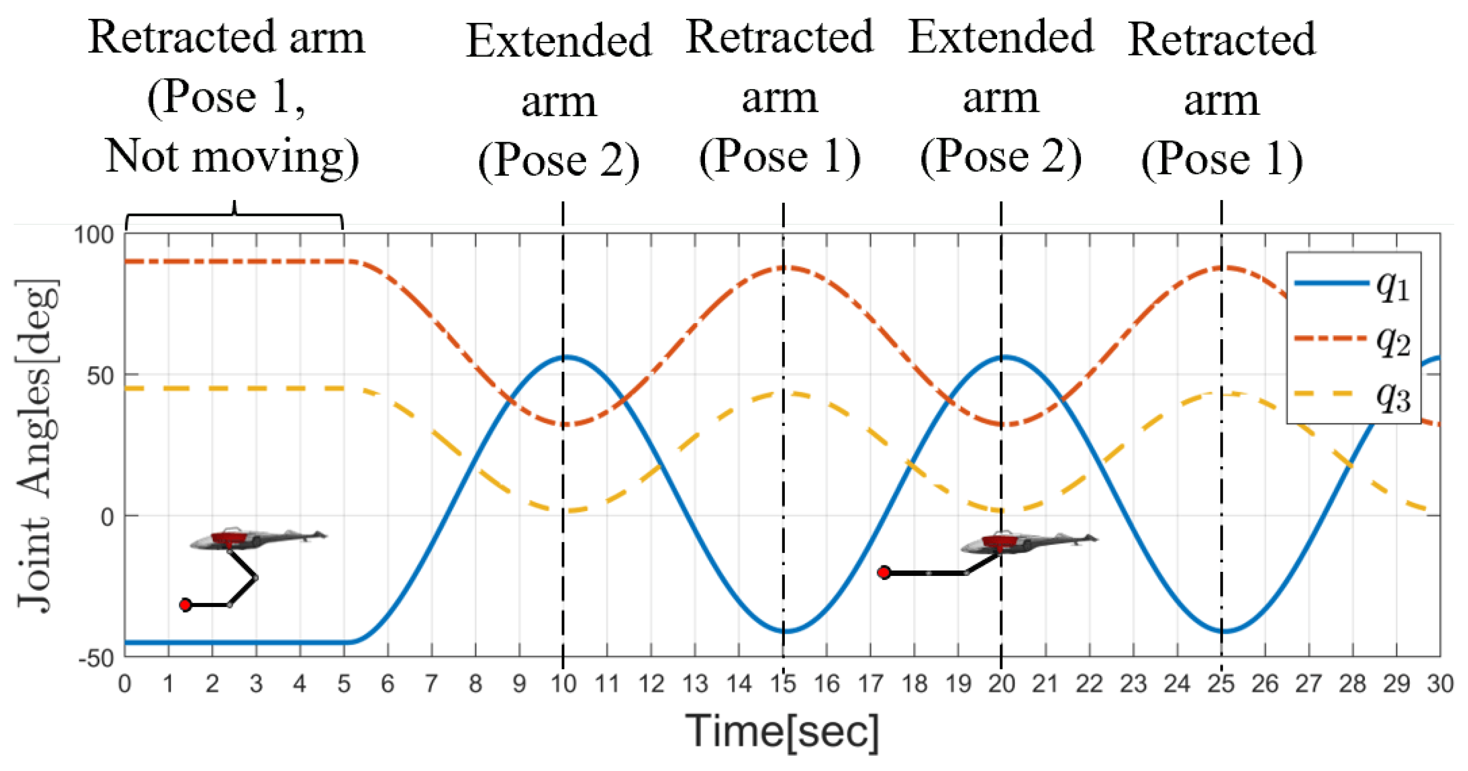
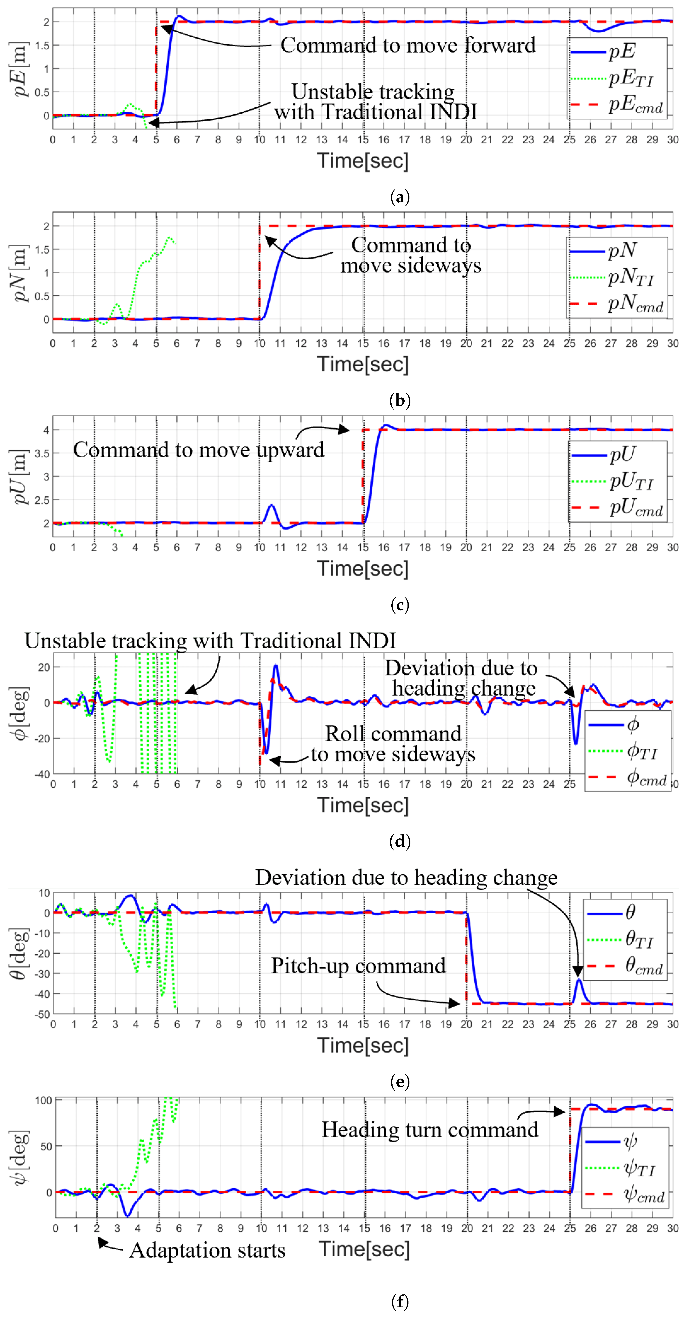
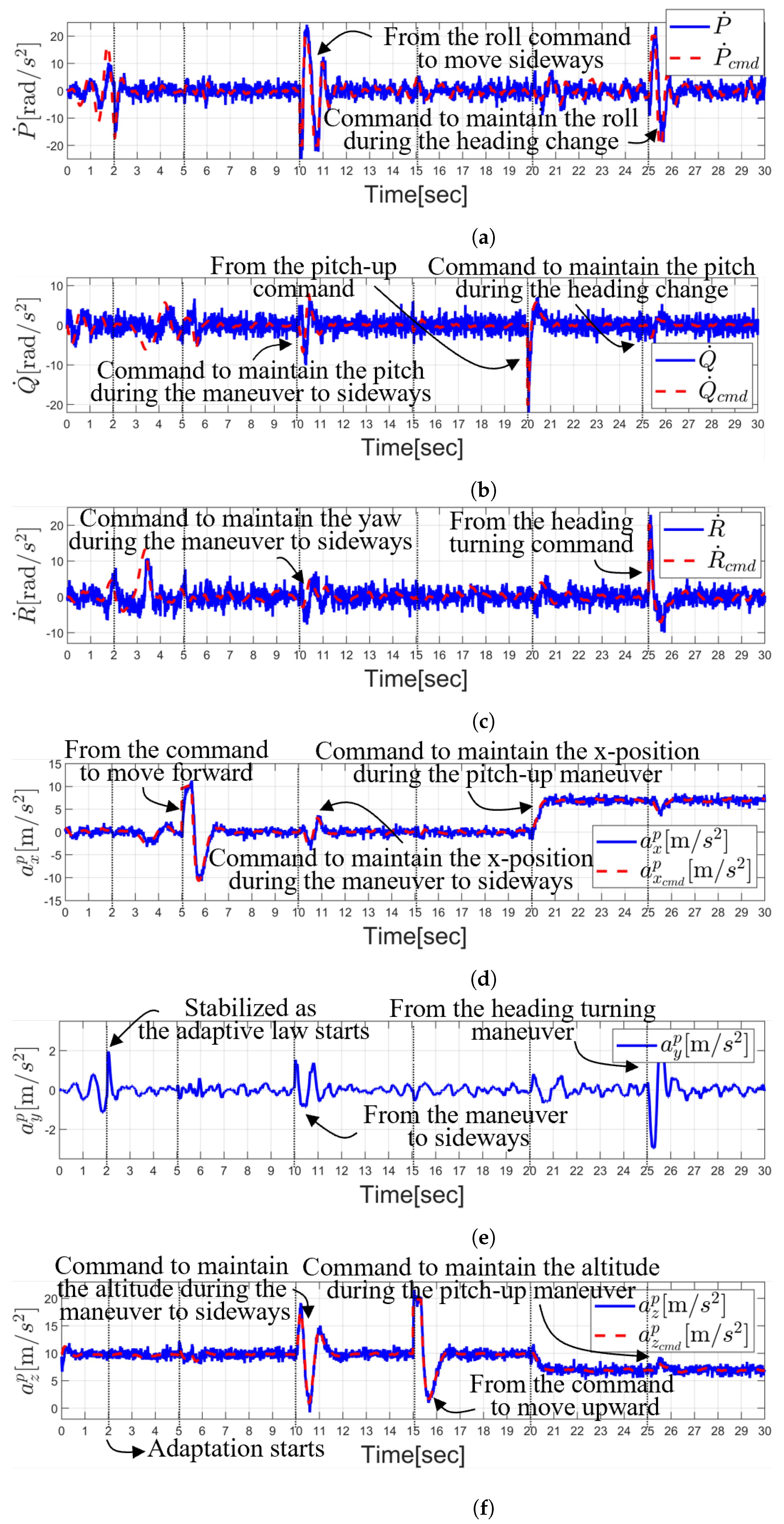
5.1. Step Response Simulation Test

For step response tests, the UAM starts in a hovering maneuver with no robot arm movement controlled, with the original INDI control having an effectiveness matrix determined based on the inertia parameters of the UAV ( G i n i 1 ). The inverse control effectiveness starts to adapt after 2 s using the proposed adaptation law. Starting from 5 s of the simulation, a step command in position and orientation is sent to the UAV at different times. Specifically, the UAV is commanded to move 2 m forward at 5 s, 2 m sideways at 10 s, and 2 m upward at 15 s. After the position commands, a −45-degree pitch attitude command is applied at 20 s, and a 90-degree yaw attitude command is applied to the UAV at 25 s. At the 5 s mark, the manipulator is commanded to continuously move, changing its pose between the two poses (Pose 1 and Pose 2) as depicted in Figure 4, where Pose 1 represents a retracted arm and Pose 2 represents an extended forward arm.
To achieve the continuous arm extension and retraction, the joint angles are commanded to change following the three joint motion curves provided in Figure 5.
It is worth noting that the manipulator moves slowly ( q ˙ m a x = 0.53 rad/s, q ¨ m a x = 0.43 rad/s2) within the angular velocity and acceleration constraints of the arm joints as detailed in Section 4.3 ( q ˙ i < 1 rad/s, q ¨ i < 10 rad/s2). This is performed to limit the generation of substantial reaction forces and torques of the arm on the UAV.
Figure 6, Figure 7 and Figure 8 provide detailed results of the above described simulation. Figure 6 presents the position ( p E , p N , and p U ) and the attitude angles of the UAV ( ϕ , θ , and ψ ). The solid lines represent the actual UAV states, while the dashed lines represent the commands applied to the UAV. The dotted line indicates the UAV states within the UAM system, controlled by the traditional INDI controller with a fixed G i n i 1 . The parameters p E , p N , and p U refer to the UAV’s position in the east, north, and upward (altitude) directions.
Figure 7 describes the acceleration states ( P ˙ , Q ˙ , R ˙ , a x P , a y P , and a z P ) of the UAV controlled by the adaptive INDI scheme.
Figure 8 represents the adaptation of the inverse of the control effective matrix throughout the simulation.
The plots on the left side (Figure 8a,c,e,g,i) show the adapted inverse control effectiveness ( G ^ 1 ) values. In contrast, the plots on the right side (Figure 8b,d,f,h,j) display the analytically calculated inverse control effectiveness ( G true 1 ) values, which are based on the true inertia parameters of the UAM and the object. The plots on the right are provided for comparison purposes, as these values are not available in real-world scenarios. The first two plots (Figure 8a,b) indicate values in the first column of the adapted and true G 1 , which play a crucial role in generating effective control commands from the P ˙ measurements. Similarly, the subsequent plots represent the second to fifth columns of the adapted and true G 1 , which are closely related to the measurements of Q ˙ , R ˙ , a x P , and a z P , respectively. The plots on the left in Figure 8 also provide the degree of change for each matrix component of G ^ 1 as the UAM flight evolves over time. From Figure 8a,c,e,g,i, it is observed that certain components of G ^ 1 undergo significant changes as the UAM changes its flight behavior while others remain unaffected. This observation indicates the significance of each element within G ^ 1 in the adaptation process.
In the initial 2 s, the UAM is controlled by the traditional INDI control scheme with the original G matrix ( G i n i 1 ). Notably, during this period, the attitude control of the UAV becomes unstable, as shown in Figure 6d and Figure 7a, where the roll attitude exhibits divergence. At 2 s of the hover-flight, the adaptive INDI algorithm initiates and the components of G ^ 1 converge to specific values within 0.5 s and continue to update thereafter. At 5 s, the UAM is commanded to move 2 m in the east (forward) direction (Figure 6a). At that time, the acceleration command in the x direction of the UAV is produced and it is properly followed as depicted in Figure 7d. During this maneuver, the second and fourth column of G ^ 1 (Figure 8g) are updated correspondingly. At 10 s, the UAV is commanded to move 2 m sideways to the north (Figure 6b), which leads to the roll angle command to the UAV (Figure 6d). Correspondingly, the angular acceleration command in the roll direction, P ˙ c m d , is generated (Figure 7a). As the values in the matrix G ^ 1 are promptly adjusted through the proposed adaptive law (Figure 8a), the control of P ˙ c m d is successfully achieved, leading to the proper control of the sideways motion ( p N ) and roll motion ( ϕ ). It should be noted that the components of the G ^ 1 matrix are also updated from the regulation of corresponding states ( Q ˙ , R ˙ , a x P , and a z P ) as shown in Figure 8. At 15 s, the UAV is commanded to increase its altitude by 2 m (Figure 6c). The linear acceleration command in the z direction is generated and controlled with the updated G ^ 1 . In this scenario, the components of G ^ 1 related to a z p are only slightly updated. At 20 s of the simulation, a pitch command of −45 degree angles (nose pointing up) is applied to the UAV (Figure 6e), resulting in the production of the corresponding angular acceleration command in the y direction of the UAV, Q ˙ . As described in Figure 7b, the Q ˙ is tightly controlled with the estimated G ^ 1 . At 25 s, the UAV is commanded to turn its heading (yaw) by 90 degrees while maintaining a pitch-up attitude (Figure 6f). The corresponding yaw angular acceleration command is produced, and adequately controlled (Figure 8e). Notably, the roll and pitch angles are agitated from the yaw maneuver due to the coupled dynamics of the vehicle, leading to the roll and pitch angle deviation from the desired values (Figure 6d,e). Accordingly, the first and third column of G ^ 1 are updated from the regulation of the roll and pitch angles (Figure 8a,c). Since the adaptive algorithm utilizes the relationship between actuator measurements and the corresponding acceleration measurements, the components of G ^ 1 primarily related to the current maneuver are updated. Consequently, not all updated components of G ^ 1 will necessarily align with the true components of G t r u e 1 at all times. This accounts for the deviation between G ^ 1 and G t r u e 1 observed in Figure 8. It can be observed from Figure 6 that the UAM system fails to stabilize its attitude when the traditional INDI control scheme is used (dotted line), leading to a loss of control.

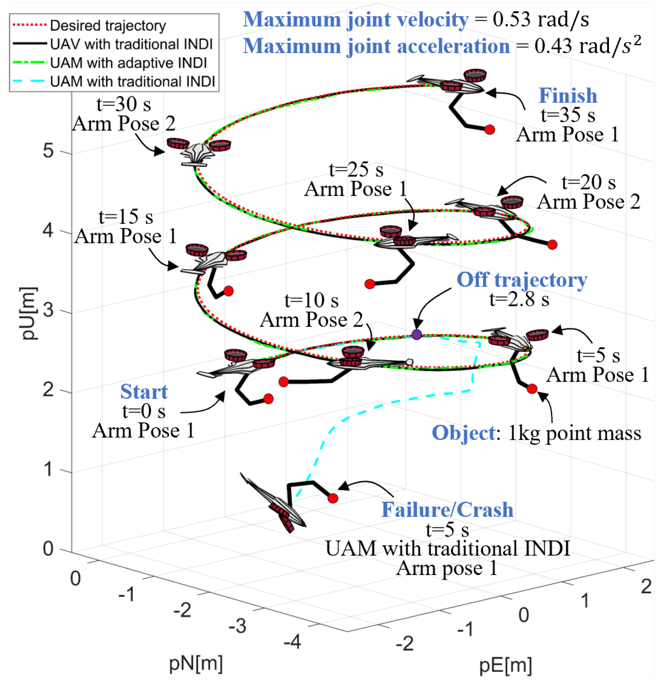
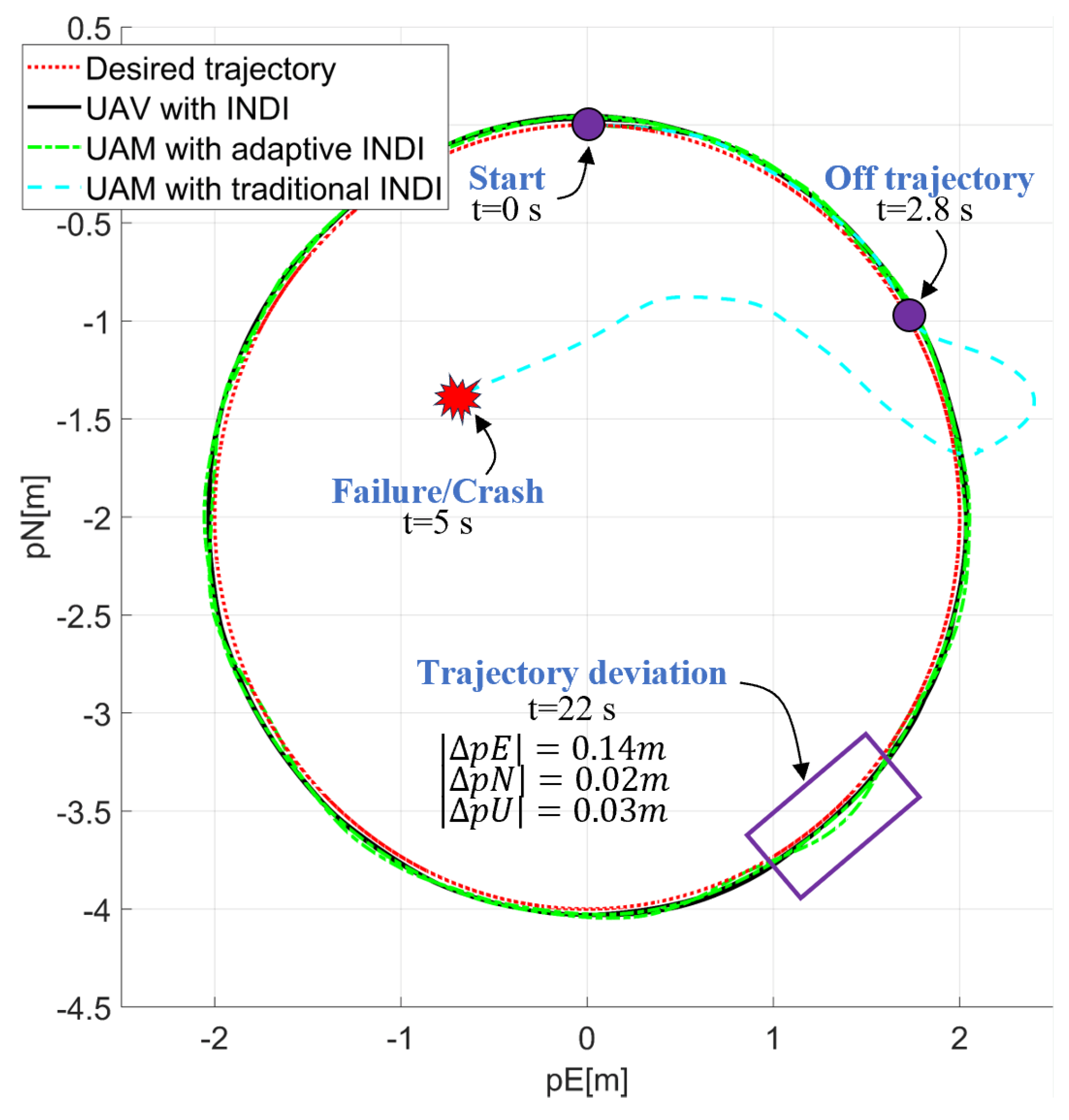
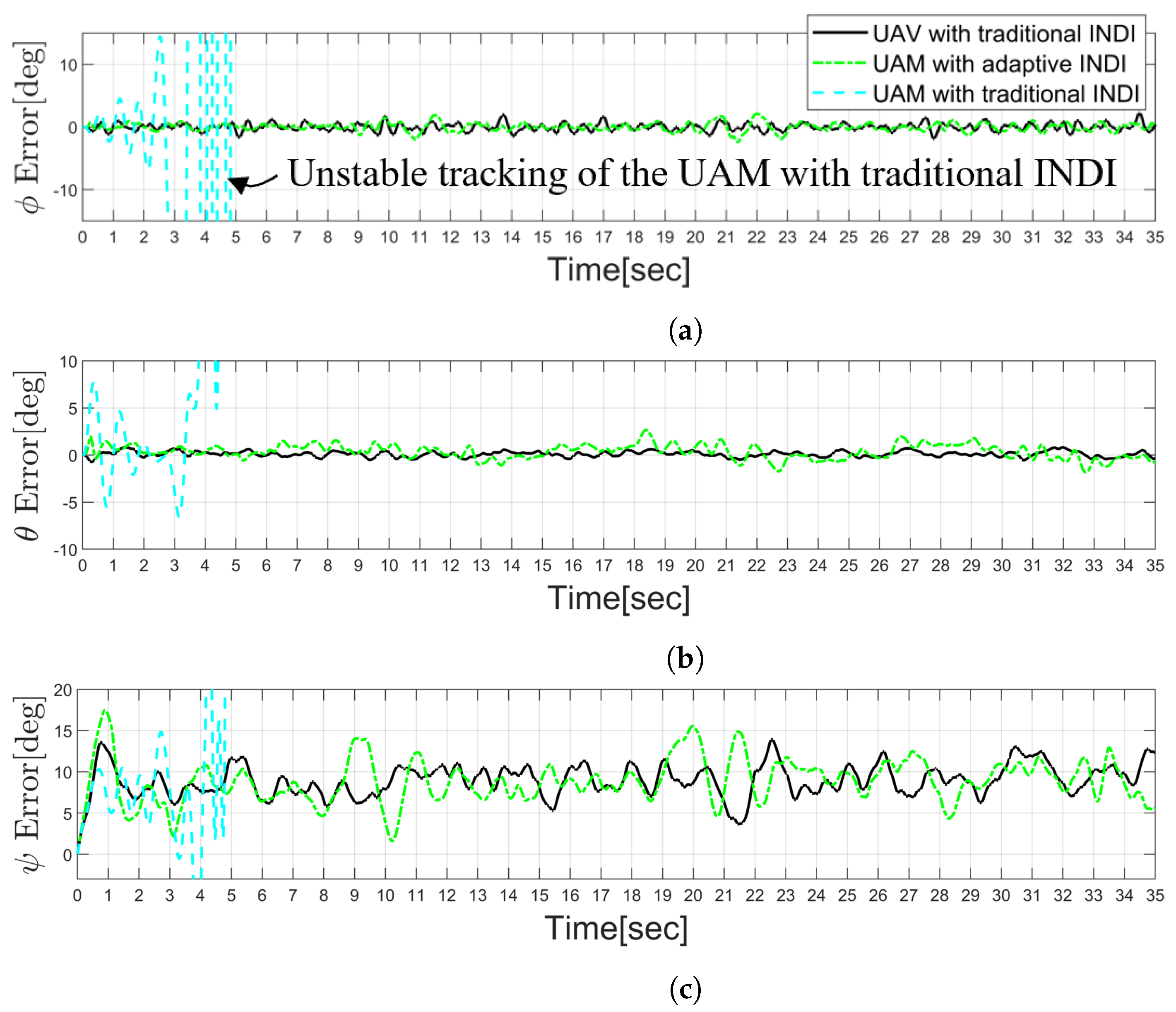
5.2. Helical Turn Climb Trajectory Tracking Flight Simulation

To analyze the trajectory tracking performance of the adaptive INDI controller, the UAM is positioned to execute a helical turn climb maneuver (Figure 9) while simultaneously managing the continuous robot arm movement between Pose 1 and Pose 2 (Figure 4). The vehicle is initially positioned at coordinates (0, 0, 2) in the inertial frame of reference, with roll, pitch, and yaw angles set at 0 degrees. Subsequently, the UAM is commanded to track the helical turn climb trajectory ( p N c m d = 2 sin 0.4 t , p E c m d = 2 cos 0.4 t 2 , p U c m d = 0.1 t + 2 , ψ c m d = 0.4 t , θ c m d = 0 , t = [ 0 , 35 ] ). During the first 5 s of the flight maneuver, the arm remains stationary. Subsequently, at 5 s, the manipulator continuously transitions between Pose 1 and Pose 2, as illustrated in Figure 9. The motion of the arm uses a max speed and acceleration of q ˙ m a x = 0.53 rad/s and q ¨ m a x = 0.43 rad/s2 following the arm motion described by Figure 5. The detailed trajectory tracking results are presented in Figure 9, Figure 10 and Figure 11. In Figure 9 and Figure 10, the dotted line represents the desired trajectory provided to the vehicle. The solid line shows the trajectory followed by the UAV without the manipulator controlled with the control effectiveness matrix derived from its own inertia parameters, G i n i 1 (traditional INDI) [28,29]. The dash-dotted line shows the trajectory of the UAM under the control of the proposed adaptive INDI control scheme, while the dashed line displays the trajectory of the UAM when it is controlled using the traditional INDI control (i.e., no adaptation). Figure 9 shows the isometric view of the trajectory with snapshots of the UAM at 5 s intervals. From the obtained results, it can be seen that the UAM’s trajectory tracking performance when controlled with the proposed adaptive INDI controller (dash-dotted line) is comparable to that of the UAV’s trajectory tracking controlled with the traditional INDI (solid line). In contrast, when the traditional INDI control with fixed control effectiveness matrix G i n i 1 is used, the UAM system fails to track the trajectory (dashed line), resulting in a loss of control. Figure 10 shows a top view of the trajectory, where trajectory tracking performance between the adaptive INDI and the traditional INDI controllers can be compared.
The trajectory followed by the UAM when controlled with the traditional INDI (dashed line) fails at 2.8 s and results in a crash at 5 s. On the other hand, the trajectory followed by the UAM when controlled with the adaptive INDI (dash-dotted line) closely matches the desired trajectory, as does the UAV trajectory with traditional INDI (solid line). However, slight deviations (e.g., deviation of ( | p E | , | p N | , | p U | ) = (0.14 m, 0.02 m, 0.03 m) at 22 s shown in Figure 10) are found, mainly caused by the reaction forces and torques from the manipulator movement, as expected. Figure 11 illustrates the attitude control errors during the trajectory tracking. The UAM with adaptive INDI control as the inner loop demonstrates performance comparable to that of UAV attitude control with traditional INDI. In contrast, the UAM fails to stabilize when controlled using traditional INDI.
As a result, the simulation results show that the proposed adaptive INDI controller can effectively control the UAM with and without arm movement, whereas the traditional INDI controller can only control the UAV itself when no arm is attached.

6. Conclusions and Future Work

This paper proposes an adaptive INDI control scheme for UAMs that relies on the acceleration responses of the vehicle to its actuation inputs. The key innovation lies in the direct estimation of the elements comprising the inverse of the control effectiveness matrix using a Kalman filter. Notably, this approach eliminates the need for any prior information regarding the manipulator movements or the size/volume and mass of the object being grasped by the manipulator. This approach effectively addresses the problem of singularities that can occur when dealing with varying manipulator dynamics as we directly estimate the inverse of G. The results show that the adaptive control law promptly adjusts the inverse of the control effectiveness, leading to a control performance that is comparable to that of controlling a UAV. However, it is important to note that the adaptation law is designed based on the UAM’s response in a quasi-static state, meaning that it does not consider the reaction forces and torques resulting from rapid manipulator movements. Extending the algorithm to handle impulsive or rapid manipulator motions, which would further enhance the UAM’s capabilities in real-world applications, is left as future work.

Author Contributions

Conceptualization, methodology, software, validation, formal analysis, investigation, resources, data curation, writing: C.P., A.R.-S. and M.B. All authors have read and agreed to the published version of the manuscript.

Funding

This research received no external funding.

Data Availability Statement

The original contributions presented in the study are included in the article, further inquiries can be directed to the corresponding author.

Conflicts of Interest

The authors declare no conflicts of interest.

Appendix A. Analytical Calculation of G

The analytical calculations of G components for Navig8-UAM are described here. In the equations below, C T i and C Q i stand for the thrust and torque coefficients of the ith propeller, which are multiplied by the square of their propeller angular velocities to obtain the thrust and torque of the propellers (i.e., C T i ω p i 2 and C Q i ω p i 2 ).
G = G 11 G 12 G 13 G 14 G 15 G 21 G 22 G 23 G 24 G 25 G 31 G 32 G 33 G 34 G 35 G 41 G 42 G 43 G 44 G 45 G 51 G 52 G 53 G 54 G 55
G 11 = I x z ( cos γ A 1 + sin γ A 0 ) + I z z ( cos γ A 2 + sin γ A 4 ) I x z 2 I x x I z z G 12 = I z z C Q 1 I x z A 2 I x z 2 I x x I z z G 13 = I x z ( cos γ A 1 + sin γ A 0 ) I z z ( cos γ A 4 sin γ A 3 ) I x z 2 I x x I z z G 14 = I z z C Q 1 I x z A 3 I x z 2 I x x I z z , G 15 = I x z C Q 2 + I z z C T 2 r o f f y I x z 2 I x x I z z
G 21 = G 23 = C Q 1 sin γ + cos γ A 0 I y y G 22 = G 24 = A 4 I y y , G 25 = A 5 I y y
G 31 = I x x ( cos γ A 1 + sin γ A 0 ) I x z ( cos γ A 2 + sin γ A 4 ) I x z 2 I x x I z z G 32 = I x z C Q 1 + I x x A 2 I x z 2 I x x I z z G 33 = I x x ( cos γ A 1 + sin γ A 0 ) + I x z ( sin γ A 4 cos γ A 3 ) I x z 2 I x x I z z G 34 = I x z C Q 1 + I x x A 3 I x z 2 I x x I z z , G 35 = I x x C Q 2 I x z C T 2 r o f f y I x z 2 I x x I z z
G 41 = G 43 = G 45 = 0 , G 42 = G 44 = C T 1 m
G 51 = G 53 = C T 1 cos γ m , G 52 = G 54 = 0 , G 55 = C T 2 m
where , A 0 = C T 1 ( r o f f x r p 1 x ) , A 1 = C Q 1 ( r o f f x r p 1 x ) A 2 = C T 1 ( r o f f y r p 1 y ) , A 3 = C T 1 ( r o f f y + r p 1 y ) A 4 = C T 1 ( r o f f z r p 1 z ) , A 5 = C T 2 ( r o f f x r p 2 x )

Appendix B. Example of the Analytical Calculation of G−1 for Navig8-UAM

Examples of the G 1 components for Navig8-UAM are shown here.
G 1 = G 11 1 G 12 1 G 13 1 G 14 1 G 15 1 G 21 1 G 22 1 G 23 1 G 24 1 G 25 1 G 31 1 G 32 1 G 33 1 G 34 1 G 35 1 G 41 1 G 42 1 G 43 1 G 44 1 G 45 1 G 51 1 G 52 1 G 53 1 G 54 1 G 55 1
G 11 1 = + I x z C Q 1 + I x x C T 1 r p 1 y B 0 , G 21 1 = B 1 B 0 G 31 1 = G 11 1 , G 41 1 = G 21 1 , G 51 1 = 0 G 12 1 = B 2 B 3 , G 22 1 = B 4 B 5 , G 32 1 = B 6 B 3 , G 42 1 = G 22 1 G 52 1 = + I y y C T 1 cos γ C Q 1 C T 2 sin γ + C T 1 C T 2 r p 1 x cos γ C T 1 C T 2 r p 2 x cos γ
Percentage difference between G 32 1 and G 12 1 :
G 12 1 G 32 1 G 12 1 × 100 = B 2 B 6 B 2 × 100 = 2 C Q 1 C Q 2 C T 1 cos γ B 7 × 100
where
B 0 = 2 ( C Q 1 2 cos γ + C T 1 2 r p 1 y 2 cos γ + C Q 1 C T 1 r o f f x sin γ C Q 1 C T 1 r p 1 x sin γ C T 1 2 r o f f z r p 1 y sin γ + C T 1 2 r p 1 y r p 1 z sin γ ) B 1 = I x x C Q 1 cos γ I x z C T 1 r p 1 y cos γ + I x x C T 1 r o f f x sin γ + I x z C T 1 r o f f z sin γ I x x C T 1 r p 1 x sin γ I x z C T 1 r p 1 z sin γ B 2 = I y y { + C Q 1 2 C T 2 cos γ + C Q 1 C Q 2 C T 1 cos γ + C T 1 2 C T 2 r p 1 y 2 cos γ C T 1 2 C T 2 r o f f z r p 1 y sin γ + C T 1 2 C T 2 r p 1 y r p 1 z sin γ + C Q 1 C T 1 C T 2 r o f f x sin γ C Q 1 C T 1 C T 2 r p 1 x sin γ } B 3 = 2 C T 2 { C Q 1 sin γ + C T 1 r p 1 x cos γ C T 1 r p 2 x cos γ } · { C Q 1 2 cos γ + C T 1 2 r p 1 y 2 cos γ + C Q 1 C T 1 r o f f x sin γ C Q 1 C T 1 r p 1 x sin γ C T 1 2 r o f f z r p 1 y sin γ + C T 1 2 r p 1 y r p 1 z sin γ } B 4 = I y y C Q 2 C T 1 2 cos γ ( r p 1 y cos γ r o f f z sin γ + r p 1 z sin γ ) B 5 = 2 C T 2 ( C Q 1 sin γ + C T 1 r p 1 x cos ( γ ) C T 1 r p 2 x cos γ ) ( C Q 1 2 cos γ + C T 1 2 r p 1 y 2 cos γ + C Q 1 C T 1 r o f f x sin γ C Q 1 C T 1 r p 1 x sin γ C T 1 2 r o f f z r p 1 y sin γ + C T 1 2 r p 1 y r p 1 z sin γ ) B 6 = I y y { + C Q 1 2 C T 2 cos γ C Q 1 C Q 2 C T 1 cos γ + C T 1 2 C T 2 r p 1 y 2 cos γ C T 1 2 C T 2 r o f f z r p 1 y sin γ + C T 1 2 C T 2 r p 1 y r p 1 z sin γ + C Q 1 C T 1 C T 2 r o f f x sin γ C Q 1 C T 1 C T 2 r p 1 x sin γ } B 7 = C Q 1 2 C T 2 cos γ + C Q 1 C Q 2 C T 1 cos γ + C T 1 2 C T 2 r p 1 y 2 cos γ C T 1 2 C T 2 r o f f z r p 1 y sin γ + C T 1 2 C T 2 r p 1 y r p 1 z sin γ + C Q 1 C T 1 C T 2 r o f f x sin γ C Q 1 C T 1 C T 2 r p 1 x sin γ

References

  1. Konert, A.; Balcerzak, T. Military autonomous drones (UAVs)—From fantasy to reality. Legal and Ethical implications. Transp. Res. Procedia 2021, 59, 292–299. [Google Scholar] [CrossRef]
  2. Shakhatreh, H.; Sawalmeh, A.H.; Al-Fuqaha, A.; Dou, Z.; Almaita, E.; Khalil, I.; Othman, N.S.; Khreishah, A.; Guizani, M. Unmanned Aerial Vehicles (UAVs): A Survey on Civil Applications and Key Research Challenges. IEEE Access 2019, 7, 48572–48634. [Google Scholar] [CrossRef]
  3. Jimenez-Cano, A.E.; Martin, J.; Heredia, G.; Ollero, A.; Cano, R. Control of an aerial robot with multi-link arm for assembly tasks. In Proceedings of the 2013 IEEE International Conference on Robotics and Automation, Karlsruhe, Germany, 6–10 May 2013; IEEE: Piscataway, NJ, USA, 2013; pp. 4916–4921. [Google Scholar] [CrossRef]
  4. Orsag, M.; Korpela, C.; Oh, P. Modeling and control of MM-UAV: Mobile manipulating unmanned aerial vehicle. J. Intell. Robot. Syst. 2013, 69, 227–240. [Google Scholar] [CrossRef]
  5. Orsag, M.; Korpela, C.; Pekala, M.; Oh, P. Stability control in aerial manipulation. In Proceedings of the 2013 American Control Conference, Washington, DC, USA, 17–19 June 2013; IEEE: Piscataway, NJ, USA, 2013; pp. 5581–5586. [Google Scholar] [CrossRef]
  6. Korpela, C.; Orsag, M.; Pekala, M.; Oh, P. Dynamic stability of a mobile manipulating unmanned aerial vehicle. In Proceedings of the 2013 IEEE International Conference on Robotics and Automation, Karlsruhe, Germany, 6–10 May 2013; IEEE: Piscataway, NJ, USA, 2013; pp. 4922–4927. [Google Scholar] [CrossRef]
  7. Orsag, M.; Korpela, C.; Bogdan, S.; Oh, P. Hybrid adaptive control for aerial manipulation. J. Intell. Robot. Syst. 2014, 73, 693–707. [Google Scholar] [CrossRef]
  8. Dief, T.N.; Yoshida, S. System identification and adaptive control of mass-varying quad-rotor. Evergreen 2017, 4, 58–66. [Google Scholar] [CrossRef]
  9. Garimella, G.; Sheckells, M.; Kim, S.; Kobilarov, M. A Framework for Reliable Aerial Manipulation. Unpublished 2018. Available online: https://asco.lcsr.jhu.edu/wp-content/uploads/2018/10/framework-reliable-aerial-1.pdf (accessed on 1 July 2022).
  10. Min, B.C.; Hong, J.H.; Matson, E.T. Adaptive robust control (ARC) for an altitude control of a quadrotor type UAV carrying an unknown payloads. In Proceedings of the 2011 11th International Conference on Control, Automation and Systems, Gyeonggi-do, Republic of Korea, 26–29 October 2011; IEEE: Piscataway, NJ, USA, 2011; pp. 1147–1151. [Google Scholar]
  11. Nicol, C.; Macnab, C.; Ramirez-Serrano, A. Robust adaptive control of a quadrotor helicopter. Mechatronics 2011, 21, 927–938. [Google Scholar] [CrossRef]
  12. Wang, C.; Nahon, M.; Trentini, M. Controller development and validation for a small quadrotor with compensation for model variation. In Proceedings of the 2014 International Conference on Unmanned Aircraft Systems (ICUAS), Orlando, FL, USA, 27–30 May 2014; IEEE: Piscataway, NJ, USA, 2014; pp. 902–909. [Google Scholar] [CrossRef]
  13. Wang, C.; Song, B.; Huang, P.; Tang, C. Trajectory tracking control for quadrotor robot subject to payload variation and wind gust disturbance. J. Intell. Robot. Syst. 2016, 83, 315–333. [Google Scholar] [CrossRef]
  14. Baraban, G.; Sheckells, M.; Kim, S.; Kobilarov, M. Adaptive parameter estimation for aerial manipulation. In Proceedings of the 2020 American Control Conference (ACC), Denver, CO, USA, 1–3 July 2020; IEEE: Piscataway, NJ, USA, 2020; pp. 614–619. [Google Scholar] [CrossRef]
  15. Lee, H.; Kim, S.; Kim, H.J. Control of an aerial manipulator using on-line parameter estimator for an unknown payload. In Proceedings of the 2015 IEEE International Conference on Automation Science and Engineering (CASE), Gothenburg, Sweden, 24–28 August 2015; IEEE: Piscataway, NJ, USA, 2015; pp. 316–321. [Google Scholar] [CrossRef]
  16. Lee, H.; Kim, H.J. Estimation, control, and planning for autonomous aerial transportation. IEEE Trans. Ind. Electron. 2016, 64, 3369–3379. [Google Scholar] [CrossRef]
  17. Park, C.; Ramirez-Serrano, A.; Bisheban, M. Estimation of Time-Varying Inertia of Aerial Manipulators Performing Manipulation of Unknown Objects. In Proceedings of the 10th International Conference of Control Systems, and Robotics (CDSR’23), Avestia, Ottawa, ON, Canada, 1–6 June 2023; p. 209. [Google Scholar] [CrossRef]
  18. Enns, D.; Bugajski, D.; Hendrick, R.; Stein, G. Dynamic inversion: An evolving methodology for flight control design. Int. J. Control. 1994, 59, 71–91. [Google Scholar] [CrossRef]
  19. Lombaerts, T.; Chu, P.; Mulder, J.A.; Joosten, D. Flight Control Reconfiguration based on a Modular Approach. IFAC Proc. Vol. 2009, 42, 259–264. [Google Scholar] [CrossRef]
  20. Simplício, P.; Pavel, M.; Van Kampen, E.; Chu, Q. An acceleration measurements-based approach for helicopter nonlinear flight control using incremental nonlinear dynamic inversion. Control. Eng. Pract. 2013, 21, 1065–1077. [Google Scholar] [CrossRef]
  21. Sun, S.; Romero, A.; Foehn, P.; Kaufmann, E.; Scaramuzza, D. A comparative study of nonlinear mpc and differential-flatness-based control for quadrotor agile flight. IEEE Trans. Robot. 2022, 38, 3357–3373. [Google Scholar] [CrossRef]
  22. Tal, E.; Karaman, S. Accurate tracking of aggressive quadrotor trajectories using incremental nonlinear dynamic inversion and differential flatness. IEEE Trans. Control. Syst. Technol. 2020, 29, 1203–1218. [Google Scholar] [CrossRef]
  23. Yang, J.; Cai, Z.; Zhao, J.; Wang, Z.; Ding, Y.; Wang, Y. INDI-based aggressive quadrotor flight control with position and attitude constraints. Robot. Auton. Syst. 2023, 159, 104292. [Google Scholar] [CrossRef]
  24. Smeur, E.J.; de Croon, G.C.; Chu, Q. Cascaded incremental nonlinear dynamic inversion for MAV disturbance rejection. Control. Eng. Pract. 2018, 73, 79–90. [Google Scholar] [CrossRef]
  25. Smeur, E.J.; Chu, Q.; De Croon, G.C. Adaptive incremental nonlinear dynamic inversion for attitude control of micro air vehicles. J. Guid. Control. Dyn. 2016, 39, 450–461. [Google Scholar] [CrossRef]
  26. Cao, S.; Shen, L.; Zhang, R.; Yu, H.; Wang, X. Adaptive Incremental Nonlinear Dynamic Inversion Control Based on Neural Network for UAV Maneuver. In Proceedings of the 2019 IEEE/ASME International Conference on Advanced Intelligent Mechatronics (AIM), Hong Kong, China, 8–12 July 2019; pp. 642–647. [Google Scholar] [CrossRef]
  27. Ahmadi, K.; Asadi, D.; Nabavi-Chashmi, S.Y.; Tutsoy, O. Modified adaptive discrete-time incremental nonlinear dynamic inversion control for quad-rotors in the presence of motor faults. Mech. Syst. Signal Process. 2023, 188, 109989. [Google Scholar] [CrossRef]
  28. Taherinezhad, M.; Ramirez-Serrano, A. An Enhanced Incremental Nonlinear Dynamic Inversion Control Strategy for Advanced Unmanned Aircraft Systems. Aerospace 2023, 10, 843. [Google Scholar] [CrossRef]
  29. Taherinezhad, M. Enhanced INDI+PID Control Strategy for Advanced Unmanned Aircraft Systems Having Highly Coupled Dynamics. Ph.D. Thesis, University of Calgary, Calgary, AB, Canada, 2023. [Google Scholar]
  30. Jansen, F.; Ramirez-Serrano, A. Agile unmanned vehicle navigation in highly confined environments. In Proceedings of the 2011 IEEE International Conference on Systems, Man, and Cybernetics, Anchorage, AK, USA, 9–12 October 2011; IEEE: Piscataway, NJ, USA, 2011; pp. 2381–2386. [Google Scholar] [CrossRef]
  31. Amiri, N.; Ramirez-Serrano, A.; Davies, R.J. Integral backstepping control of an unconventional dual-fan unmanned aerial vehicle. J. Intell. Robot. Syst. 2013, 69, 147–159. [Google Scholar] [CrossRef]
  32. Majnoon, M.; Samsami, K.; Mehrandezh, M.; Ramirez-Serrano, A. Mobile-Target Tracking via Highly-Maneuverable VTOL UAVs with EO Vision. In Proceedings of the 2016 13th Conference on Computer and Robot Vision (CRV), Victoria, BC, Canada, 1–3 June 2016; IEEE: Piscataway, NJ, USA, 2016; pp. 260–265. [Google Scholar] [CrossRef]
  33. Yavari, M.; Gupta, K.; Mehrandezh, M.; Ramirez-Serrano, A. Optimal real-time trajectory control of a pitch-hover UAV with a two link manipulator. In Proceedings of the 2018 International Conference on Unmanned Aircraft Systems (ICUAS), Dallas, TX, USA, 12–15 June 2018; IEEE: Piscataway, NJ, USA, 2018; pp. 930–938. [Google Scholar] [CrossRef]
  34. Sieberling, S.; Chu, Q.; Mulder, J. Robust flight control using incremental nonlinear dynamic inversion and angular acceleration prediction. J. Guid. Control. Dyn. 2010, 33, 1732–1742. [Google Scholar] [CrossRef]
  35. Keesman, K.J.; Keesman, K.J. Time-varying Dynamic Systems Identification. In System Identification: An Introduction; Springer: London, UK, 2011; pp. 195–221. [Google Scholar] [CrossRef]
  36. Kalman, R.E.; Bucy, R.S. New results in linear filtering and prediction theory. J. Basic Eng. 1961, 83, 95–108. [Google Scholar] [CrossRef]
Figure 1. The Navig8-UAV and hypothetical Navig8-UAM: (a) The Navig8-UAV; (b) The hypothetical Navig8-UAM.
Aerospace 11 00671 g001
Figure 2. Schematic diagram of the Navig8-UAM.
Aerospace 11 00671 g002
Figure 3. Block diagram of the proposed adaptive INDI controller for UAMs.
Aerospace 11 00671 g003
Figure 4. Manipulator poses during the simulation.
Aerospace 11 00671 g004
Figure 5. Joint angles of the manipulator during the simulation.
Aerospace 11 00671 g005
Figure 6. Position and attitude control of the UAV during the simulation: (a) UAV position control in the east direction; (b) UAV position control in the north direction; (c) UAV position control in the upward direction; (d) UAV roll angle control; (e) UAV pitch angle control; (f) UAV yaw angle control.
Aerospace 11 00671 g006
Figure 7. Acceleration control of the UAV during the simulation: (a) UAV angular acceleration control in the x direction of the UAV frame; (b) UAV angular acceleration control in the y direction of the UAV frame; (c) UAV angular acceleration control in the z direction of the UAV frame; (d) UAV linear acceleration control in the x direction of the UAV frame; (e) UAV linear acceleration control in the y direction of the UAV frame; (f) UAV linear acceleration control in the z direction of the UAV frame.
Aerospace 11 00671 g007
Figure 8. Components of the inverse control effectiveness matrix during the simulation: (a) 1st column of the adapted G 1 ; (b) 1st column of the true G 1 ; (c) 2nd column of the adapted G 1 ; (d) 2nd column of the true G 1 ; (e) 3rd column of the adapted G 1 ; (f) 3rd column of the true G 1 ; (g) 4th column of the adapted G 1 ; (h) 4th column of the true G 1 ; (i) 5th column of the adapted G 1 ; (j) 5th column of the true G 1 .
Aerospace 11 00671 g008
Figure 9. Side view of the helical trajectory achieved by the UAM.
Aerospace 11 00671 g009
Figure 10. Top view of the helical trajectory achieved by the UAM.
Aerospace 11 00671 g010
Figure 11. Attitude control errors during the helical trajectory tracking simulation: (a) roll angle control error; (b) pitch angle control error; (c) yaw angle control error.
Aerospace 11 00671 g011
Table 1. Equality conditions of the components of G 1 .
1st Column2nd Column3rd Column5th Column
G 11 1 = G 31 1 G 12 1 G 32 1 G 13 1 = G 33 1 G 25 1 = G 45 1
G 21 1 = G 41 1 G 22 1 = G 42 1 G 23 1 = G 43 1
G 51 1 = 0 G 53 1 = 0
Table 2. Sign conditions of the components of G 1 .
Positive G 11 1 G 14 1 G 23 1 G 34 1 G 42 1 G 52 1
Negative G 12 1 G 22 1 G 24 1 G 31 1 G 32 1 G 43 1 G 44 1 G 54 1
Table 3. Size and inertia parameters of the UAM components.
Size [m]Mass [kg] I xx  [kg·m2] I yy  [kg·m2] I zz  [kg·m2] I xz  [kg·m2] I xy  [kg·m2] I yz  [kg·m2]
Navig8-UAVlength: 1.05.00.06670.14920.20190.014700
width: 0.8
height: 0.2
Each arm linkagelength: 0.30.50.00370.00370000
Object (sphere)radius: 0.051.00.0010.0010.001000
Disclaimer/Publisher’s Note: The statements, opinions and data contained in all publications are solely those of the individual author(s) and contributor(s) and not of MDPI and/or the editor(s). MDPI and/or the editor(s) disclaim responsibility for any injury to people or property resulting from any ideas, methods, instructions or products referred to in the content.

