Assembly Simulation and Optimization Method for Underconstrained Frame Structures of Aerospace Vehicles

Abstract

Aerodynamic contour dimensional accuracy is very important for the stable and safe flight of aerospace vehicles. Nevertheless, due to the influence of various factors such as material properties, machining and manufacturing deviations, and assembly and installation deviations, key structural geometric dimensions are frequently exceeded. Therefore, this paper investigates a data-driven combined vector loop method (VLM)–Skin Model Shapes (SMS) method to realize aerospace vehicle structural geometric accuracy analysis; assembly optimization targeting contour deviation is also achieved. Tests are carried out on a typical aerospace vehicle’s underconstrained structural workpieces to validate the effectiveness of the proposed method.

1. Introduction

The working conditions of aerospace vehicles often cover a wide speed domain and various complex environments [1,2]. In order to accommodate these diverse working conditions, the designs of aerospace vehicles adopt complex curved aerodynamic contours and a large number of composite materials, putting forward new challenges on the manufacture and assembly of space vehicles [3,4,5]. For aerospace vehicles, contour accuracy is a key parameter for determining the performance of the product. However, the manufacturing characteristics of composite parts requires greater dimensional accuracy than metal parts, necessitating secondary processing during the production [5,6,7,8]. Achieving the assembly accuracy requirements of multi-part components often requires iterative grinding of the parts, leading to further degradation in production efficiency.

Therefore, how to reflect the actual manufacturing error in the assembly’s accumulated deviation, predict the accumulation process of assembly deviation in key parts in advance, and realize quality process control and data-driven adjustments based on a prediction model has become the key to improving the assembly efficiency. To address this issue, this paper applies the geometric deviation modeling method to the assembly adjustment of aerospace vehicles. Various geometric deviation modeling methods have been studied. Desrochers et al. [9] proposed a matrix model from the TTRS model by using the homogeneous transform matrix to describe the tolerance zones and the clearances in 3D space. Desrochers et al. [10] also introduced topologically and technologically related surfaces (TTRSs), where parts are represented by a successive binary tree formed by associated elementary surfaces. Chase and Gao [11,12] proposed the direct linearization method (DLM) based on the vector loop method (VLM) for 2D/3D tolerance analysis. Dimensional deviation and assembly deviation are comprehensively represented by vectors. Laperriere [13] combined the Jacobian model [14] with the Torsor model [15] to introduce the unified Jacobian–Torsor model. Mujezinovic [16] proposed the Tolerance-Map (T-Map) model. A hypothetical Euclidean point space is established, whose size and shape reflect the variational possibilities of the target feature. Some other methods, such as feature-based topologically and technologically related surfaces (FTTRSs) [17] and Manufacturing-Map (M-Map) [18], etc., are derived from the above methods.

However, most of the existing methods simplify the complex surface morphology of the part to an ideal surface, allowing easy description and analysis using regular geometric features. But this also results in the loss of surface morphology information and assembly analysis accuracy. The geometric deviation caused by the morphology of the mating surfaces of different parts during assembly is non-negligible for high-precision systems [19]. With the development of computer technology, studies use numerical methods to represent morphology features caused by manufacturing and perform assembly simulation analysis to address the above problems. One of the most representative approaches is Skin Model Shapes (SMS), proposed by Schleich [20]. This method utilizes discrete surfaces and finite data to describe and characterize workpiece surfaces’ morphologies, allowing for precise assembly analysis [21,22].

The problem of geometric deviation control, especially contour deviation, in aerospace vehicle frame assembly is highly prominent in production. In order to realize high-precision analysis of geometric deviations, and to improve productivity by increasing the assembly qualification rate, this paper presents an assembly simulation method combining VLM and SMS to optimize contour surface accuracy: Assembly dimensional deviation transfer analysis is realized by VLM, and SMS is adopted for surface morphological deviation modeling and mating analysis.

The rest of this paper is structured as follows. Section 2 describes the main idea of the VLM-SMS modeling method. Section 3 introduces the details of the aerospace vehicle frame structure assembly deviation simulation and optimization method. In Section 4, the experimental process and test results are demonstrated. Section 5 presents the conclusions of this work.

2. Data-Driven VLM-SMS Modeling Approach

It is very important to bring real-time measurement data into the analysis model for assembly-oriented analysis. Therefore, a data-driven analytical method combined with VLM-SMS is demonstrated for aerospace vehicle assembly. Elastic deformation on geometric accuracy is not considered for the following reasons: (1) the target structure is an underconstrained structure; assembly internal forces are negligible. (2) Parts made of composite materials have high specific strength and high specific stiffness.

2.1. Vector Loop-Based Assembly Deviation Transfer Model

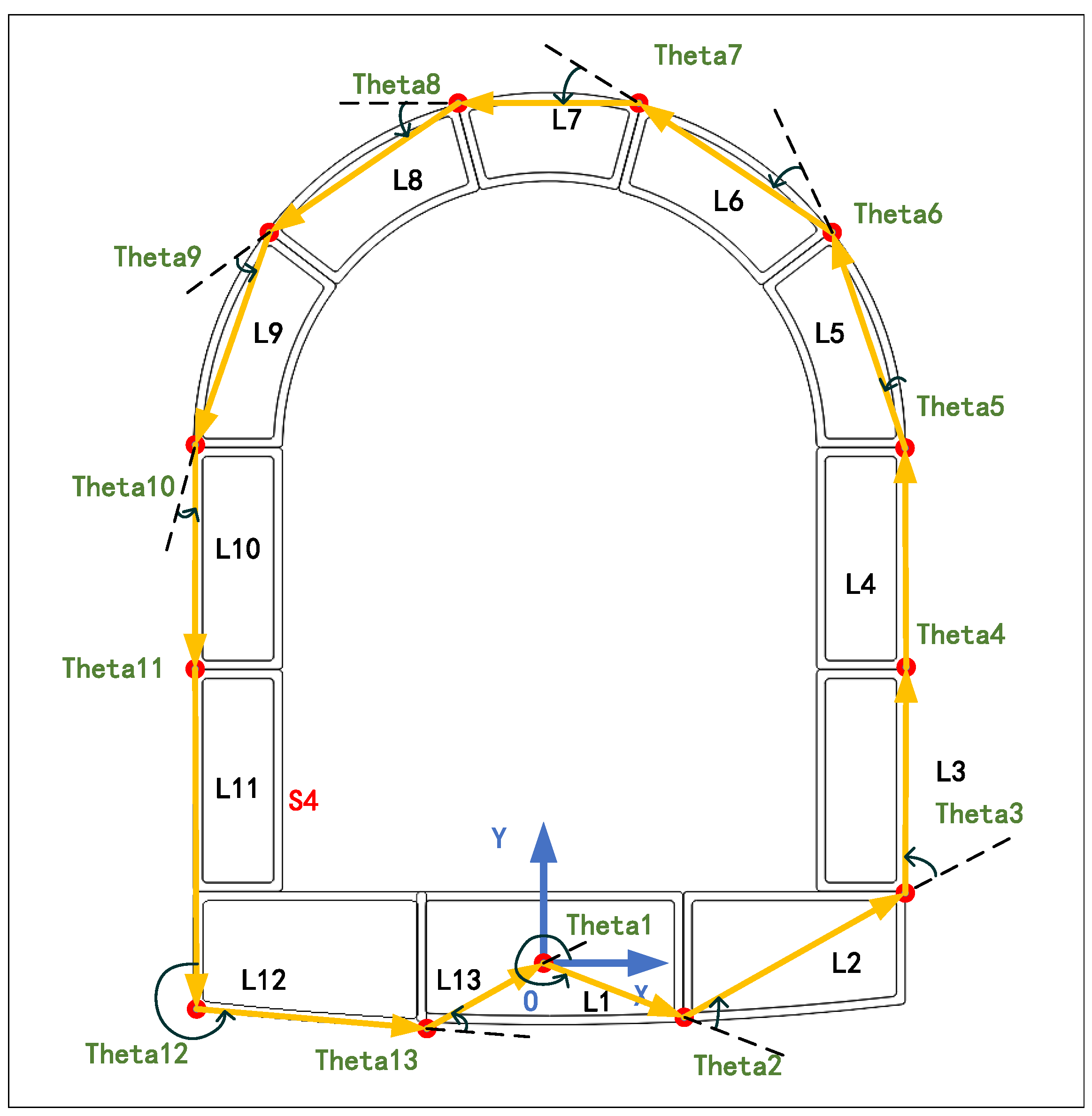
The VLM method has advantages in terms of computational speed, brought by the direct linearization method (DLM) [23], which is important for assembly stage analysis. The basic idea of the method is to use vectors to represent geometric features in the assembly, as is shown in Figure 1.

The assembly deviation analysis method based on the VLM consists of several steps [24]. First, establishing the assembly kinematic constraint equations. Second, calculating the derivation evaluation matrix from the above kinematic constraint equations. Third, linearizing the assembly constraint equations and using DLM to enable rapid evaluation of the deviation matrix. Finally, incorporating the measured data to the established model.

Since the frame assembly of an aerospace vehicle is performed on a flat surface, the assembly process can be simplified to assembly in 2D space. The rotational translation matrix in 2D space can be expressed by

$$\left[{\Theta }_i\right]=\left[\begin{array}{ccc}cos\left({\theta }_i\right)& -sin\left({\theta }_i\right)& 0\\ sin\left({\theta }_i\right)& cos\left({\theta }_i\right)& 0\\ 0& 0& 1\end{array}\right]$$

(1)

$$\left[L_i\right]=\left[\begin{array}{ccc}1& 0& l_i\\ 0& 1& 0\\ 0& 0& 1\end{array}\right]$$

(2)

A closed vector loop in 2D space [12] is expressed by

$$\left[{\Theta }_1\right]\left[L_1\right]\left[{\Theta }_2\right]\left[L_2\right]\dots \left[{\Theta }_i\right]\left[L_i\right]\dots \left[{\Theta }_n\right]\left[L_n\right]\left[{\Theta }_f\right]=\left[I\right]$$

(3)

where:

• $\left[{\Theta }_i\right]$ is the rotation matrix;
• $\left[L_i\right]$ is the translation matrix at joint i;
• $\left[{\Theta }_f\right]$ is the final rotation required to bring the loop to closure;
• $\left[I\right]$ is the identity matrix;
• n is the total number of vectors.

Equation (1) represents the closed loop formed by a series of rotations and translations.

Kinematics in 2D space always has three degrees of freedoms (DOFs), including two translational DOFs and one rotational DOF. A 2D vector loop should satisfy constraints on those DOFs. Based on the small displacement assumption, kinematic equations can be linearized, expressed by

$$\delta H_i=\sum _{j=1}^n{\displaystyle \frac{\partial H_i}{\partial s_j}}\delta s_j+\sum _{k=1}^m{\displaystyle \frac{\partial H_i}{\partial u_k}}\delta u_k=0,(i=x,y,{\theta }_x)$$

(4)

where:

• $\delta s_j$ are variations in the manufactured dimensions and angles $(j=1\dots n);$
• $\delta u_k$ are variations in the dependent assembly variables $(k=1\dots m),$ representing the kinematic adjustments required to produce closure;
• $H_x,H_y$ are the translational constraints and $H_{{\theta }_x}$ is the rotational constraint in the $x, y$, and z directions, respectively;
• $\delta H_i$ is the resultant assembly variation in the corresponding global direction, here equal to zero.

Assembly constraint derivatives are obtained by the perturbation method [23]: A translational deviation $\Delta L$ is added to the nominal translational variation L, represented by

$$\left[{\theta }_1\right]\left[L_1\right]\left[{\theta }_2\right]\left[L_2\right]\dots \left[{\theta }_i\right][L_i+\Delta L_i]\dots \left[{\theta }_n\right]\left[L_n\right]\left[{\theta }_f\right]=\{\Delta X\Delta Y\}$$

(5)

An angular deviation $\Delta {\theta }_i$ is added to the nominal rotational variations $\Delta \theta$, represented by

$$\left[{\theta }_1\right]\left[L_1\right]\left[{\theta }_2\right]\left[L_2\right]\dots [{\theta }_i+\Delta {\theta }_i]\left[L_i\right]\dots \left[{\theta }_n\right]\left[L_n\right]\left[{\theta }_f\right]=\{\Delta X\Delta Y\}$$

(6)

where:

• $\{\Delta X\Delta Y\}$ is the closure deviation vector caused by assembly derivatives.

By omitting the higher-order perturbations, the first-order Taylor series expansion of assembly constraint Equation (2) is rewritten in matrix form as

$$\left\{\delta H\right\}=\left[A\right]\left\{\delta V\right\}+\left[B\right]\left\{\delta U\right\}=\{\Theta \}$$

(7)

where:

• $\left\{\delta H\right\}$ represents the vector of the clearance variations;
• $\left\{\delta V\right\}$ represents the vector of the variations in the manufactured variables;
• $\left\{\delta U\right\}$ represents the vector of the variations in the assembly variables;
• $\left[A\right]$ represents the matrix of the first-order partial derivatives of the manufactured variables;
• $\left[B\right]$ represents the matrix of the first-order partial derivatives of the assembly variables;
• $\{\Theta \}$ represents zero vector.

Matrices $\left[A\right]$ and $\left[B\right]$ are determined by

$$\left\{A_i\right\}=\{{\displaystyle \frac{\partial H_x}{\partial v_i}},{\displaystyle \frac{\partial H_y}{\partial v_i}},{\displaystyle \frac{\partial H_{\theta }}{\partial v_i}}\}$$

(8)

$$\left\{B_i\right\}=\{{\displaystyle \frac{\partial H_x}{\partial u_i}},{\displaystyle \frac{\partial H_y}{\partial u_i}},{\displaystyle \frac{\partial H_{\theta }}{\partial u_i}}\}$$

(9)

Assuming $\left[B\right]$ is a full-rank matrix, then $\left\{\delta U\right\}$ can be further obtained from Equation (2):

$$\left\{\delta U\right\}=-{\left[B\right]}^{-1}\left[A\right]\left\{\delta V\right\}$$

(10)

In Equation (10), matrix$\left[A\right]$ and matrix $-{\left[B\right]}^{-1}$ impose the geometric sensitivity to component variations $\delta X$, and the adjustments along the correct kinematic joint axes to achieve closure, respectively. The above equation indicates the relationship between assembly variations $\left\{\delta U\right\}$ and manufactured variables $\left\{\delta X\right\}$.

When a described system is over-determined, the matrix $\left[B\right]$ is singular, a least-squares fit must be applied to solve Equation (2):

$$\left\{\delta U\right\}=-{\left({\left[B\right]}^T\left[B\right]\right)}^{-1}{\left[B\right]}^T\left[A\right]\left\{\delta V\right\}$$

(11)

From Equation (11), it can be concluded that two main factors determine the geometrical deviation of a system: (1) The geometrical configuration and deviation of the manufactured structure, represented by matrix A and matrix $\delta V$. (2) The geometrical configuration of the assembled structure, represented by matrix B. For certain systems with a fixed structure, the geometric deviation can be evaluated by determining only the deviations due to manufacturing and assembly. For ease of description, a sensitivity matrix S is defined by

$$\left[S\right]=-{\left[B\right]}^{-1}\left[A\right]\left(determined\right)$$

(12)

$$\left[S\right]=-{\left({\left[B\right]}^T\left[B\right]\right)}^{-1}{\left[B\right]}^T\left[A\right](over-determined)$$

(13)

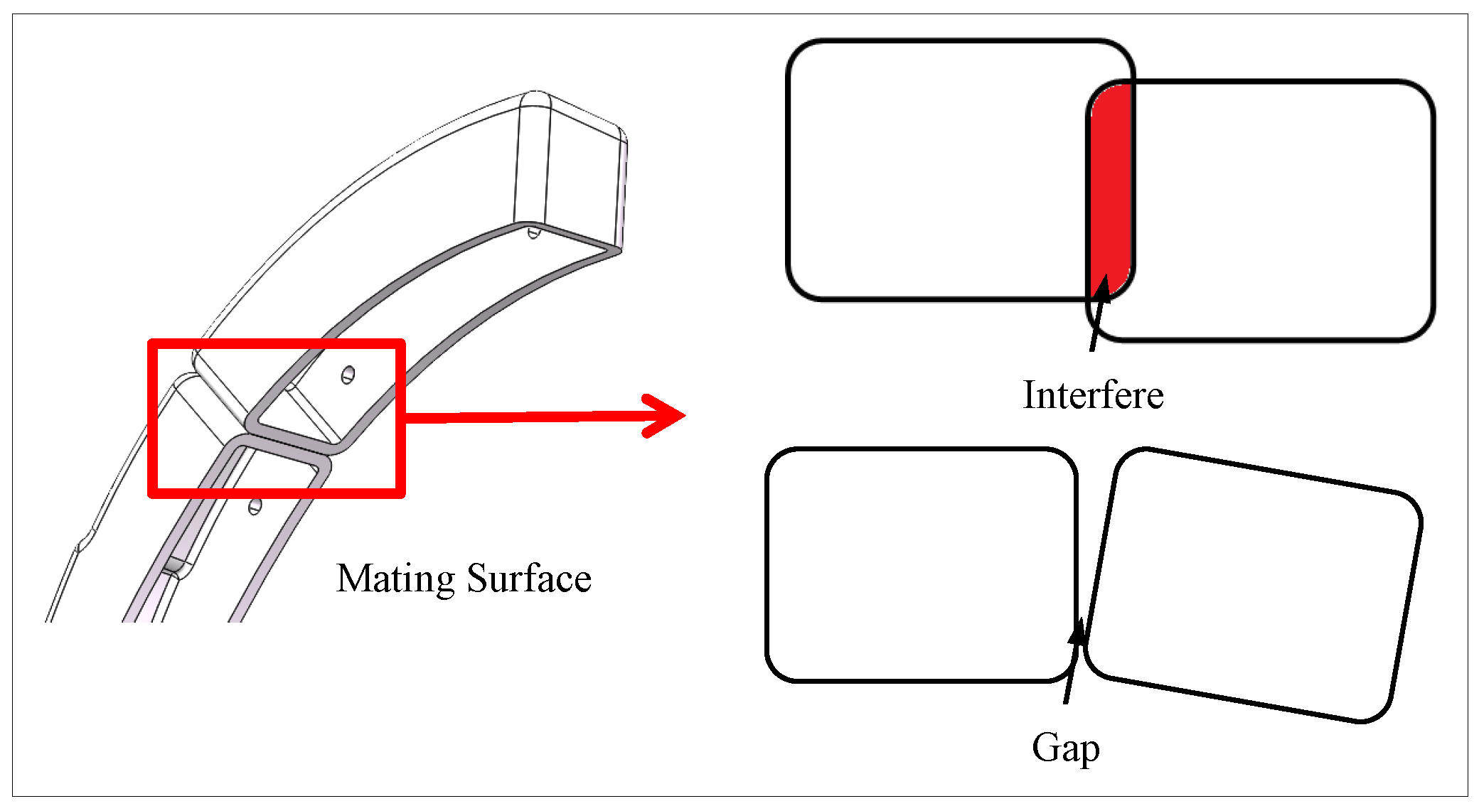
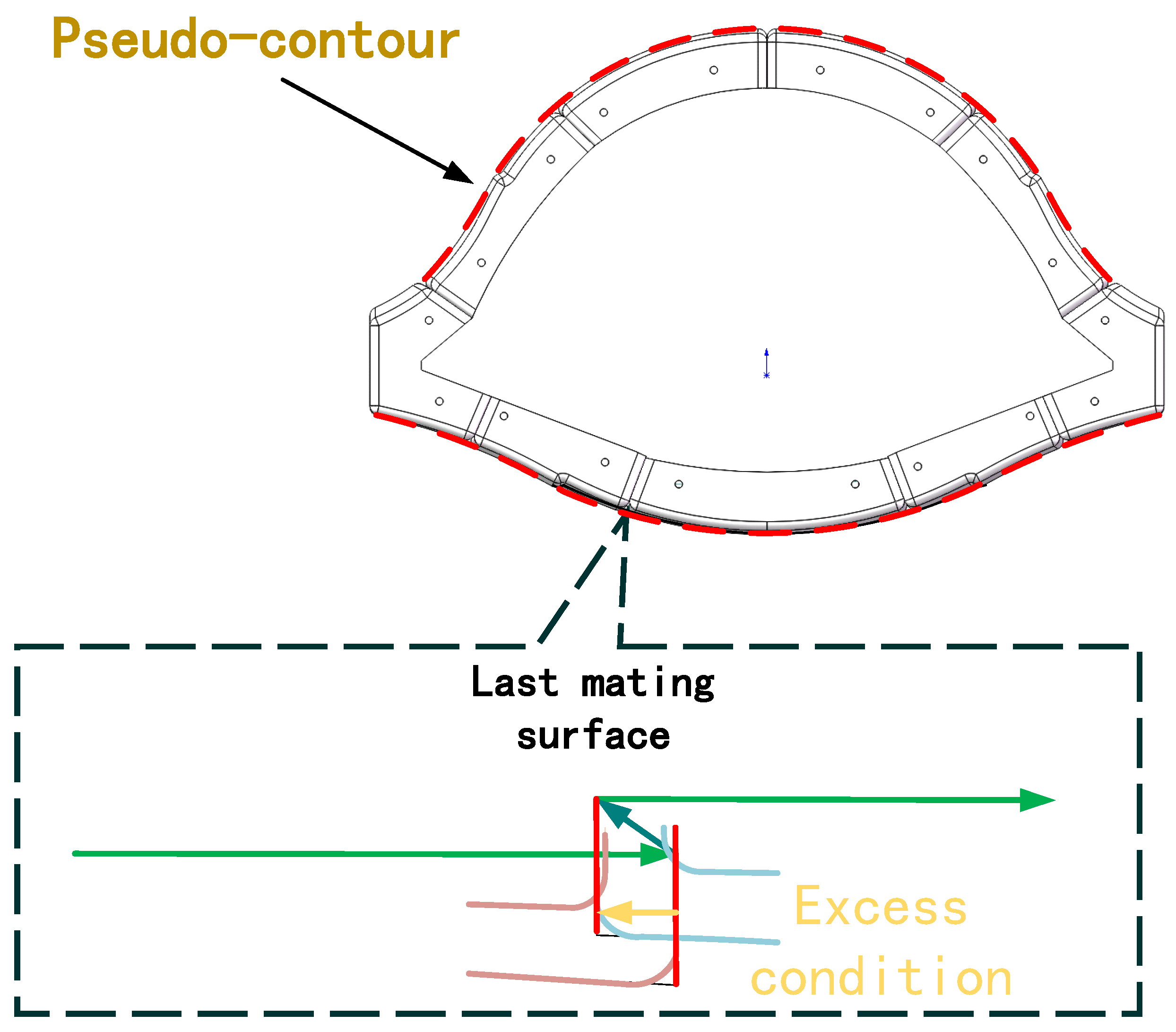
2.2. SMS-Based Assembly Mating Surface Deviation Modeling

According to the previous section, determining manufacturing assembly deviations is crucial for analyzing assembly geometric deviations. In order to realize high-precision simulation, it is vital to consider the impact of surface morphology deviations caused by manufacturing and complex surface mating status on assembly accuracy. Therefore, the concept of SMS is applied to the modeling of manufacturing and assembly deviations.

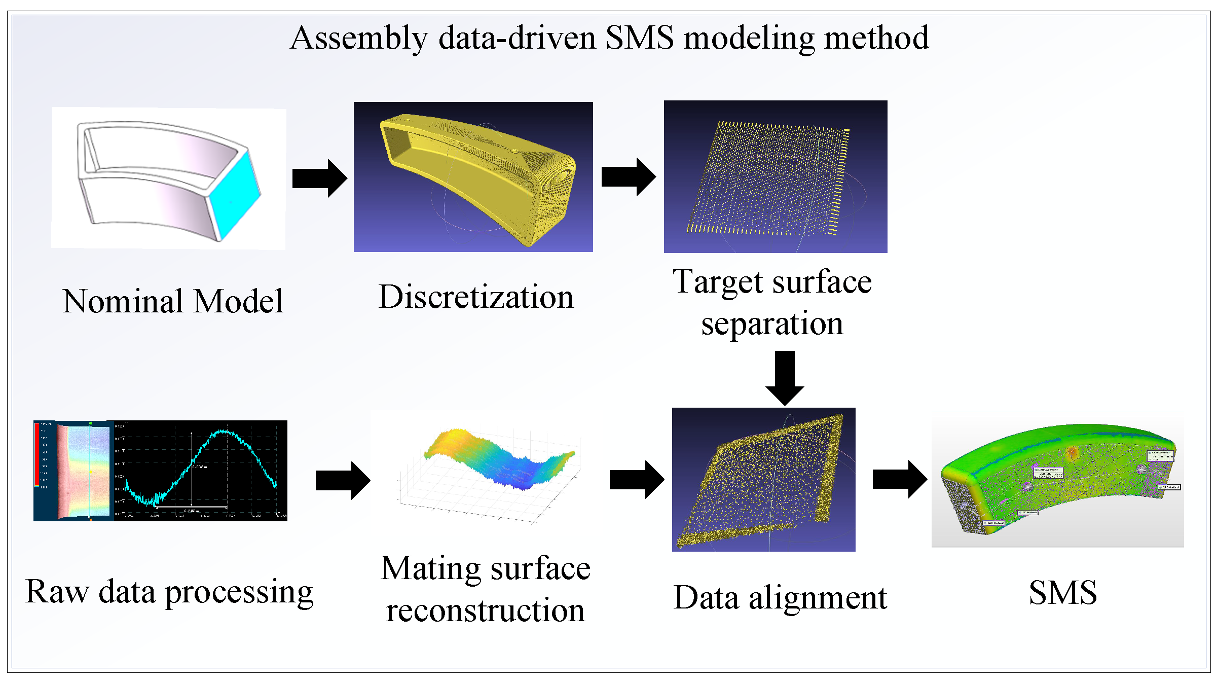
The concept of SMS is derived from a skin model, which is defined as a geometrical model of the physical boundary between a product and its external environment [25]. It is a non-ideal continuous surface model with an infinite number of points conceived to satisfy the tolerance specification, and serves as a bridge between the nominal surface model and the real surface of the workpiece. SMS is a discrete surface model with a finite number of data points extracted from the skin model. It can be used to analyze and predict the impact of a given tolerance value on the performance of the product at a later stage and to visualize deviations in real time [20], as shown in Figure 2.

The application of Skin Model Shapes is highly dependent on the observable sources of the workpieces’ geometric deviations. Previous work on obtaining observable geometric deviations and simulating SMS is limited to two stages [20]: the prediction stage, where only the designed tolerances are available; and the observation stage, where the simulation’s deviation and limited observed data are available.

By summarizing the existing methodologies, the following features are present:

• Predicting qualification rates for batch products, rather than individual products.
• Quality prediction for future assemblies based on previously available data, rather than on-site analysis.
• Tolerance design in the design phase rather than assembly stage parameter optimization.

Existing SMS methods do not meet the demands of the assembly phase. Thus, this work proposes a new assembly-stage Skin Model Shape simulation method, as illustrated in Figure 3.

The establishment of an assembly-phase-oriented SMS consists of the following main steps:

First, workpieces’ SMSs, in the form of point clouds, are discretized from the CAD design models. The resolution of the discrete point cloud is determined by the measurement equipment and analysis accuracy.

Second, the point clouds belonging to the mating surface geometric features, such as plane, cylinder, and curved surface, are extracted and separated from the SMSs.

Meanwhile, based on the requirements of different assembly processes, the appropriate equipment is utilized to measure mating surfaces, and the collected data undergo filtering and de-noising. It is important to note that various scales of micro-geometric features exist on the surface, including roughness, waviness, and lay errors. Overly rough surface profiles can lead to inaccurate simulation results, while overly detailed surface morphology reduces computational efficiency. Thus, it is necessary to normalise the scale of the measured data to ensure the validity and efficiency of the simulation at the same time. According to Scheleich’s work [20], the effect of roughness on assembly accuracy is negligible for precision-machined surfaces. Thus, in this work, assembly simulations only consider the lay and waviness level of surface deviation.

Then, the collected data are aligned, with separated mating face point clouds, and the processed surfaces are joined back to the nominal model.

If the effect of measurement errors of the measurement equipment on the assembly needs to be taken into account, the measurement uncertainty can also be added to the point cloud data in the form of random errors.

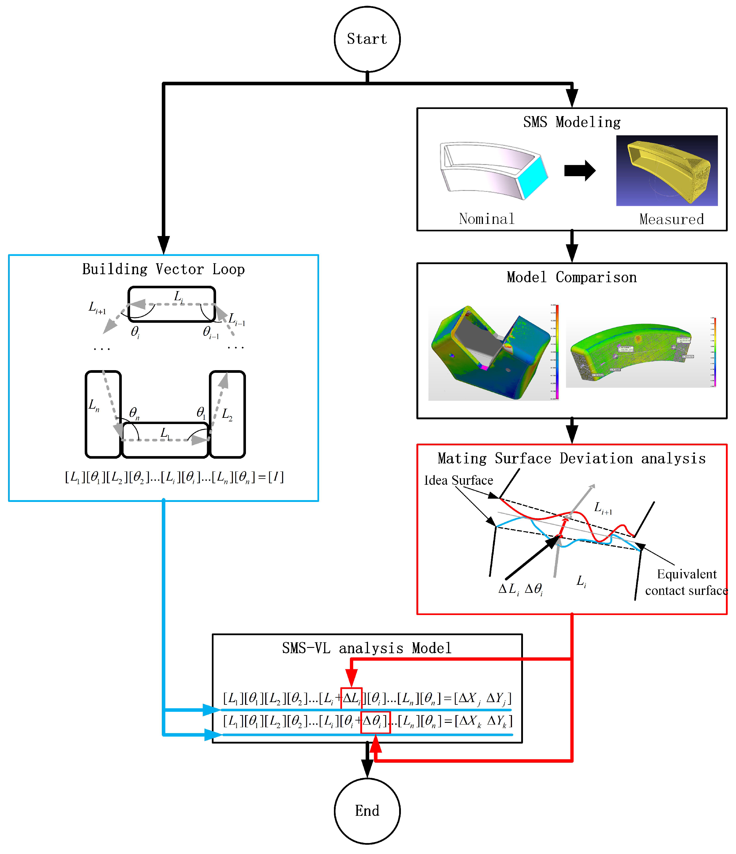
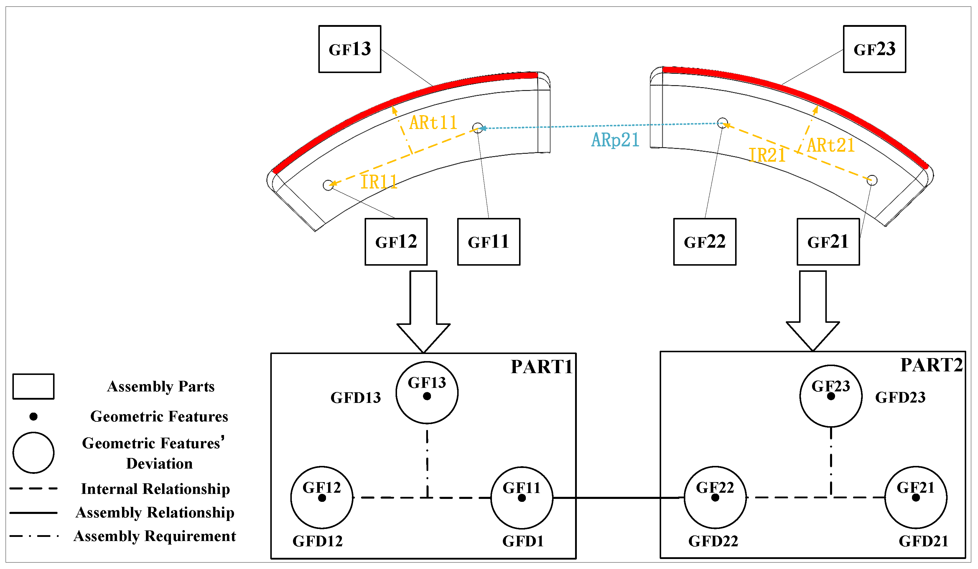
2.3. VLM-SMS Assembly Deviation Analysis Method

In current VLM, the deviation of translation $\Delta L_i$ and the deviation of rotation $\Delta {\theta }_i$ are determined by designed tolerances, rendering it incapable of meeting the needs of on-site assembly analysis. In addition, traditional geometric deviation models that use ideal geometric features, such as plane and cylinder, to represent the assembly mating surfaces can only consider rotational and translational features, without considering the effect of the mating surface morphology on the assembly.

Therefore, in this work, VLM is combined with SMS. The implementation steps of the SMS-VLM method and the analysis process are shown in Figure 4.

First, based on VLM, a vector loop in the form of Equation (1) is generated according to the nominal geometric parameters of the target structure. Meanwhile, using measured data, the SMS of the structure in the form of point clouds is generated. Then, generating the equivalent contact planes based on SMS, here a least-squares fit is applied.

By this method, the dimensional deviations, including translation deviation $\Delta L_i$ and rotation deviation $\Delta {\theta }_i$, of mating surfaces can be obtained by on-site measured data. Surface morphology deviations are analyzed by SMS, and then, incorporated into the established vector loop in the form of Equations (5) and (6).

3. Simulation and Optimization of Aerospace Vehicle Frame Structure Assembly Deviation

3.1. Analysis of Assembly Mating Surfaces’ Deviation Forms

A typical structural frame of a space vehicle is assembled from multiple boxed parts, as shown in Figure 5.

For this structure, the contour of its outer surface is one of the most important assembly quality indicators. In the actual assembly process, due to deviations caused by manufacturing, clearances or interference may occur on the mating surfaces of the parts, as is shown in Figure 6. While gaps are easily dealt with by adding filler material, interferences, which need to be adjusted through a more complex grinding process, are of greater concern: insufficient grinding of the mating surface leads to insufficient adjustment of the contour, while excessive grinding reduces the structural strength. Therefore, the main focus in modeling is on the surface morphology and geometric deviations rather than the clearance, and using the data-driven assembly deviation analysis model to determine the correlation between the contour and the mating surface adjustment value when interference occurs, and complete the trimming before assembly, so as to improve the efficiency and prevent part failure.

To ensure the regularity of the assembly data, assembly features are classified into five types, as shown in Figure 7, inspired by the works of Hultman [26] and Bao [27]: geometric features (GFs), geometric feature deviation (GFD), internal relationship (IR), assembly relationship (ARp), and assembly requirement (ARt). Detailed definitions of these assembly features are introduced in previous work [24] and are not repeated here.

In this VLM, IR is determined by the geometric parameters determined by the manufacturing process, while the ARp is jointly determined by the manufacturing process and the assembly process. Therefore, the state of the contour can be changed by grinding the parts or adjusting the assembly parameters.

3.2. Underconstrained Frame Structure Assembly Simulation

Due to the unconstrained state of the structure during the assembly process, the presence of multiple DOFs makes it is difficult to perform direct simulation. Therefore, in combination with the actual assembly process in the field, the following assumptions are made for the ease of the assembly simulation.

Assumption 1.

All parts are always in the same plane during assembly. As described in Section 2.1, this assumption is made based on the actual assembly process. By this assumption, the kinematic equations of the part are ensured to be in 2D space, with a maximum of three DOFs.

Assumption 2.

During the assembly process, the mating surfaces of two neighboring parts always fit together, and each part can only translate in the direction of the mating surface $\Delta L_u$ of the previous part. The relationship between mating surface translation $\Delta L_u$ and normal direction translation of the reference hole connection lines $\Delta L_t$ is expressed by:

$$\Delta L_t=\Delta L_{u}sin\left(\theta \right)$$

(14)

where θ is the angle between the mating surface and the normal direction of the connecting reference hole line, as shown in Figure 8.

Assumption 3.

The change in the normal direction of the reference hole connection lines $\Delta L_n$ is also affected by the grinding amount of its mating surfaces, and the grinding amount $\Delta L_v$ exists only in the direction normal to the grinding surfaces, as is shown in Figure 8.

In this case, the relationships between the contour maximum excess value $\Delta N_c$ and part translation adjustment $\Delta L_t$, grinding amount $\Delta L_v$, and mating surface assembly deviation $\Delta L_u$ can be expressed as:

$$\Delta L_t=Max(\Delta N_c)$$

(15)

$$\Delta L_t=\Delta L_{v}sin\left({\theta }_v\right)+\Delta L_{u}cos\left({\theta }_v\right)$$

(16)

Assumption 4.

According to the assembly process, a fixed assembly sequence is applied in the simulation, as shown in Figure 9.

3.3. Contour-Oriented Assembly Optimization Method

Combining the above assumptions with the VLM-SMS method, contour deviation analysis can be realized for an aerospace vehicle. However, due to the multitude of adjustable parameters, it is difficult to find the best solution to ensure both accuracy and efficiency at the same time.

To address the above question, an optimization method combining pseudo-constraints with a sensitivity matrix is proposed.

The main idea of this method is to create a pseudo-constraint of the contour in the virtual space so that all the part contours during the assembly simulation do not exceed this pseudo-contour. Assuming that the positive direction is from outside the contour plane to inside the contour plane, then

$$Max\left(N_c\right)-\Delta N_c\le O$$

(17)

where:

• $Max\left(N_c\right)$ represents the maximum permissible excess value of the contour.
• O stands for a zero matrix.

The virtual assembly does not consider grinding the first time, only adjusting the assembly relationship so that the part meets the pseudo-constraints, which means

$$\Delta L_t=\Delta L_{u}cos\left({\theta }_v\right)$$

(18)

The mating surfaces’ status during assembly is determined by the method presented in Section 2.3. If by adjusting the parts’ translation adjustment $\Delta L_u$ alone, all the contour extreme points can be met within the permissible range of the pseudo-constraint contour, and no interference exists on all the mating surfaces, then it means that the group of parts does not need to be repaired. Conversely, if adjustments are insufficient and interference is present, then this group of parts requires grinding.

Criterion: For an assembly structure in 2D space, its vector loop is represented by

$$\Delta H=A\Delta L_v+B\Delta L_u$$

(19)

where:

• $\Delta H$ represents the variation in the closed loop established in the vector loop;
• $A,B$ are determined by the structure’s geometric parameters and VLM model;
• $\Delta L_v$ is the grinding adjustment amount on each mating surface;
• $\Delta L_u$ is the assembly adjustment amount on each mating surface.

The geometric relationship between its contour excess value $\Delta N_c$ and $\Delta L_v$, $\Delta L_u$ is expressed as

$$\Delta N_c=f(\Delta L_v,\Delta L_u)$$

(20)

When $\Delta L_v$ remains constant, there exists a set of assembly parameters $\Delta L_u\in \mathbb{R}$ which satisfies Equations (17) and (21) at the same time,

$$\Delta H\le O$$

(21)

where:

• O stands for a zero matrix;
• $\Delta H_i>O$ indicates interference in the ith mating surface, while $\Delta H_i<O$ indicates clearance in the ith mating surface.

This means that no adjustment is needed for the grinding amount $\Delta L_v$ to complete an assembly that meets the contouring requirements.

There are many methods to determine whether a point is within the permissible range. Here, the method used is the ray casting method [28]. This involves drawing a ray from the target point and examining the number of intersections between this ray and all the edges of the polygon. If there is an odd number of intersections, it indicates the point is inside; if there is an even number of intersections, it indicates the point is outside. The implementation details of the algorithm can be found in the literature [28] and will not be reiterated here.

If a group of parts needs to be ground, for the ease of distributing the grinding amount, it is assumed that there is no interference or clearance on any faces except the last one during the assembly. Then, dimensional deviation of the parts may lead to an excess condition (clearance or interference) on the last mating surface, as is shown in Figure 10. If interference occurs, it means that some parts need to be ground.

Then, based on the sensitivity matrix determined by the established VLM, it is possible to determine the contribution of each mating surface to the amount of clearance or interference on the last face by Equation (10). By identifying the mating face with the largest contribution, the minimum number of surfaces to be ground and the grinding amount for each surface can be determined.

4. Case Study

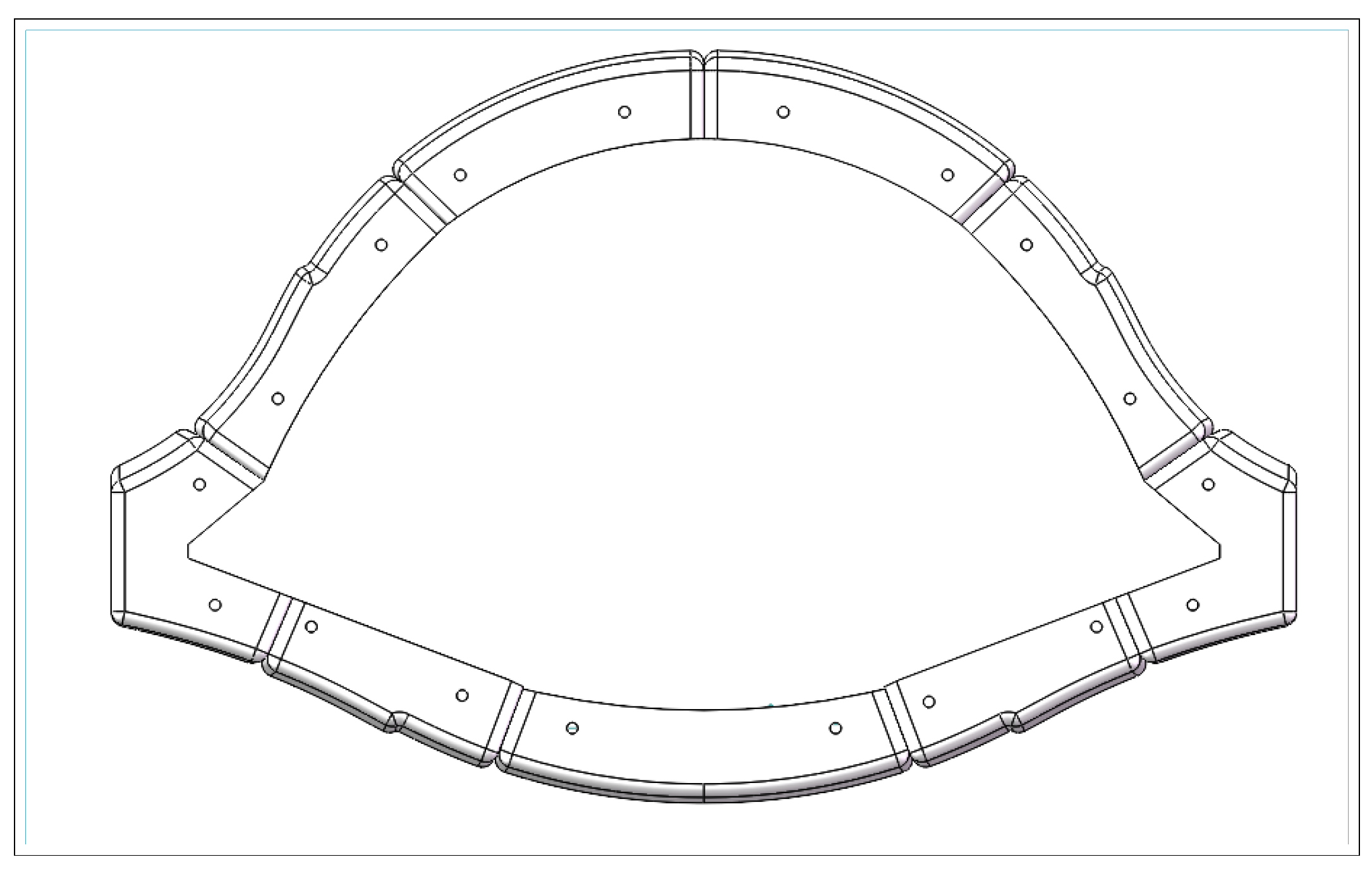
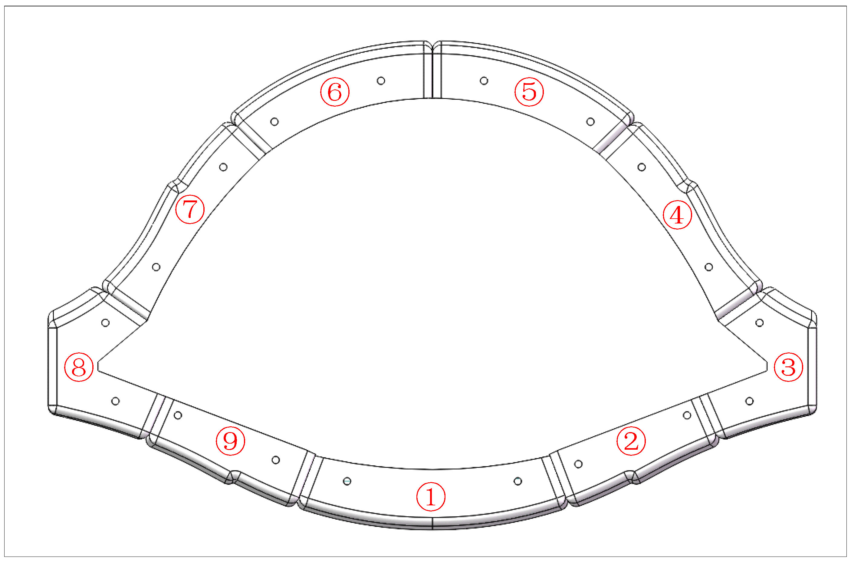
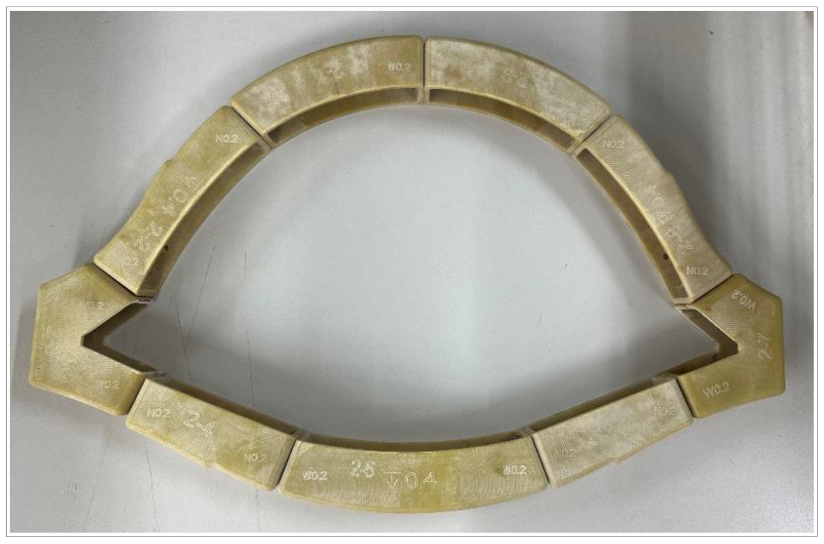
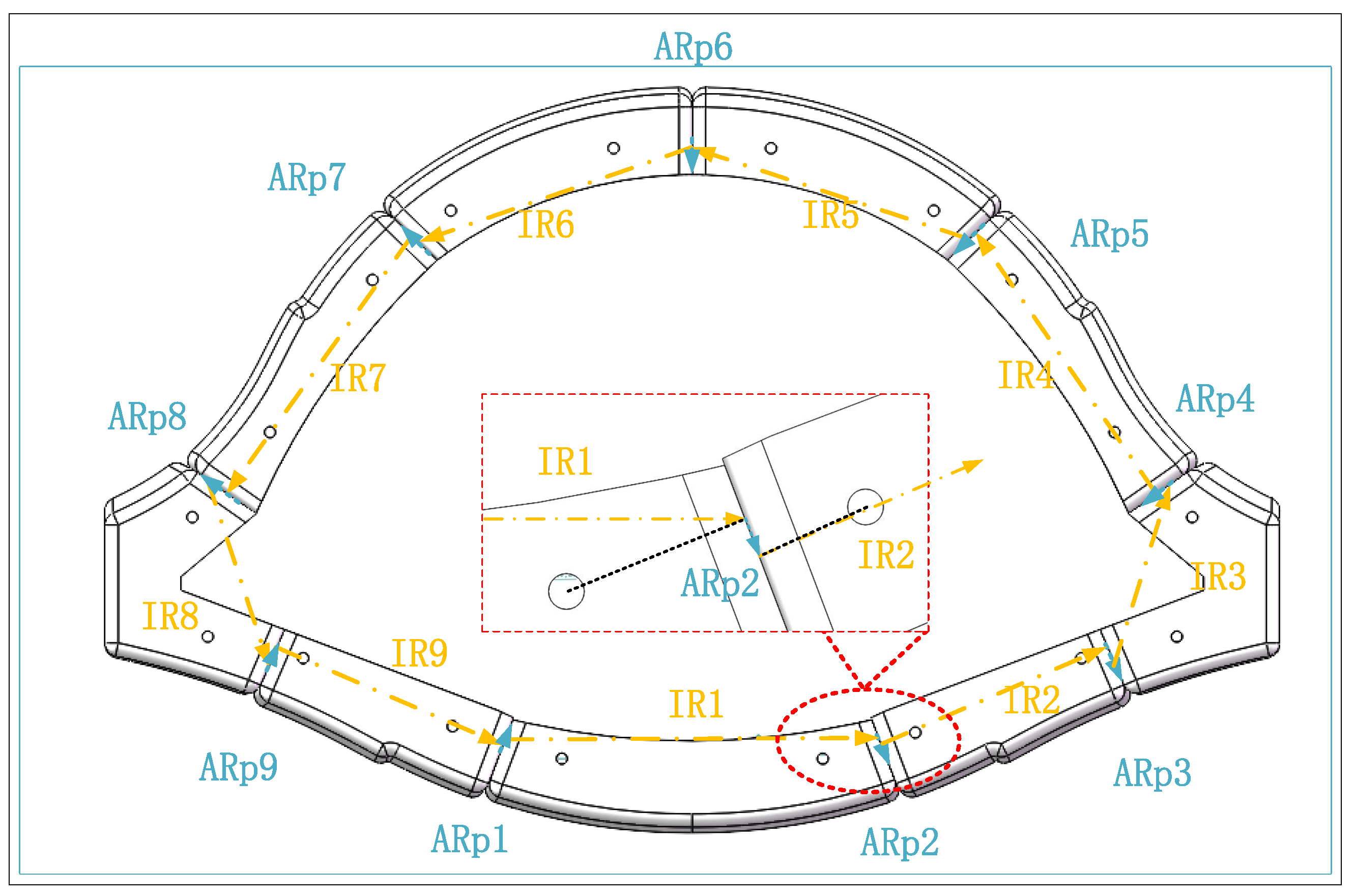
For the assembly experiments, a set of aerospace vehicle structural assembly test parts is designed, as is shown in Figure 11. Each part has two positioning holes on its lower surface. The outer contour surfaces, upper and lower surfaces, and left and right mating surfaces are all refined. The upper and lower surfaces are parallel, and the left and right contact surfaces are perpendicular to the upper and lower surfaces. When assembling the parts, the mating surfaces of each part are adjustable, and the contour surface is the optimization target.

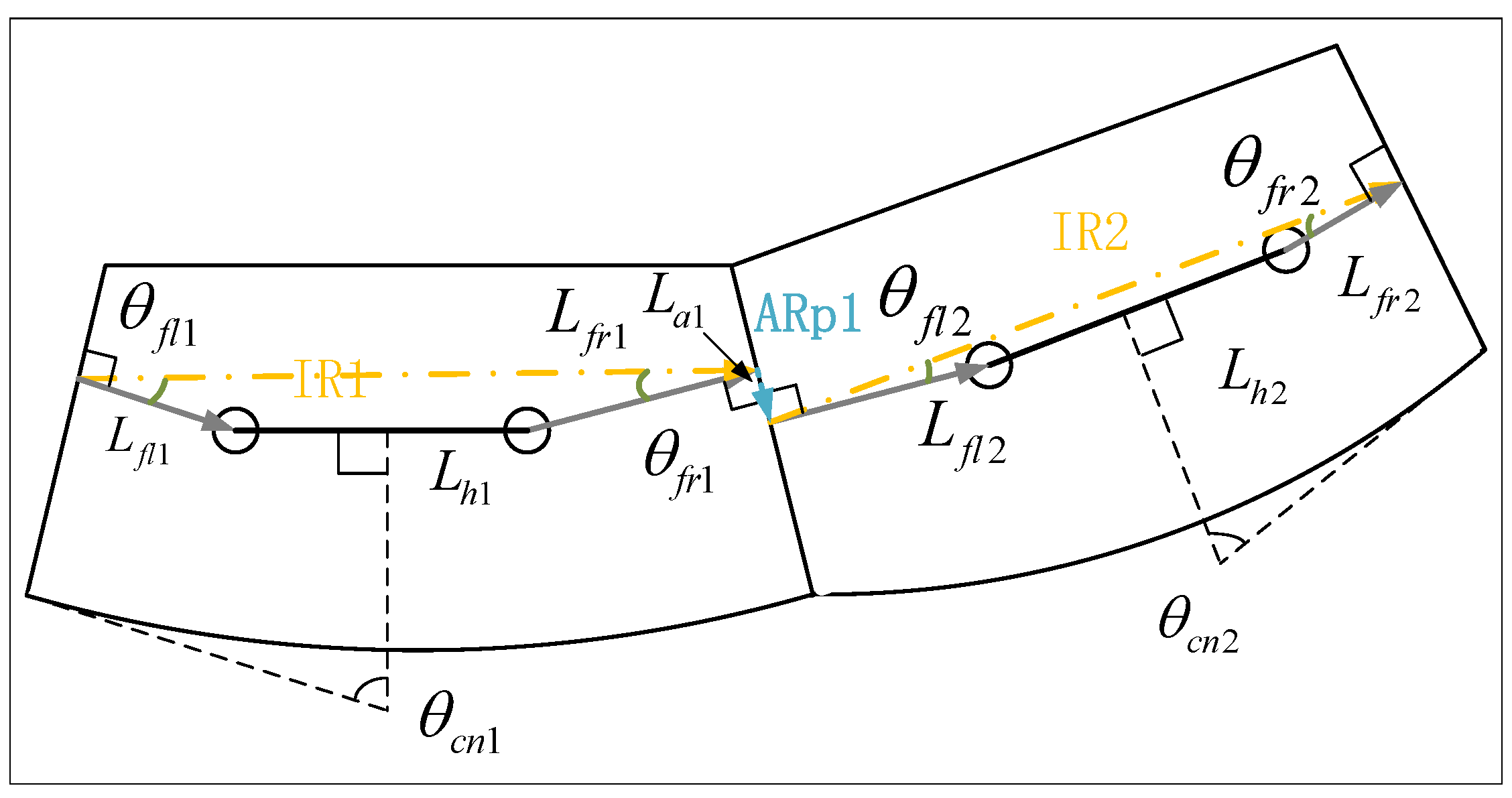
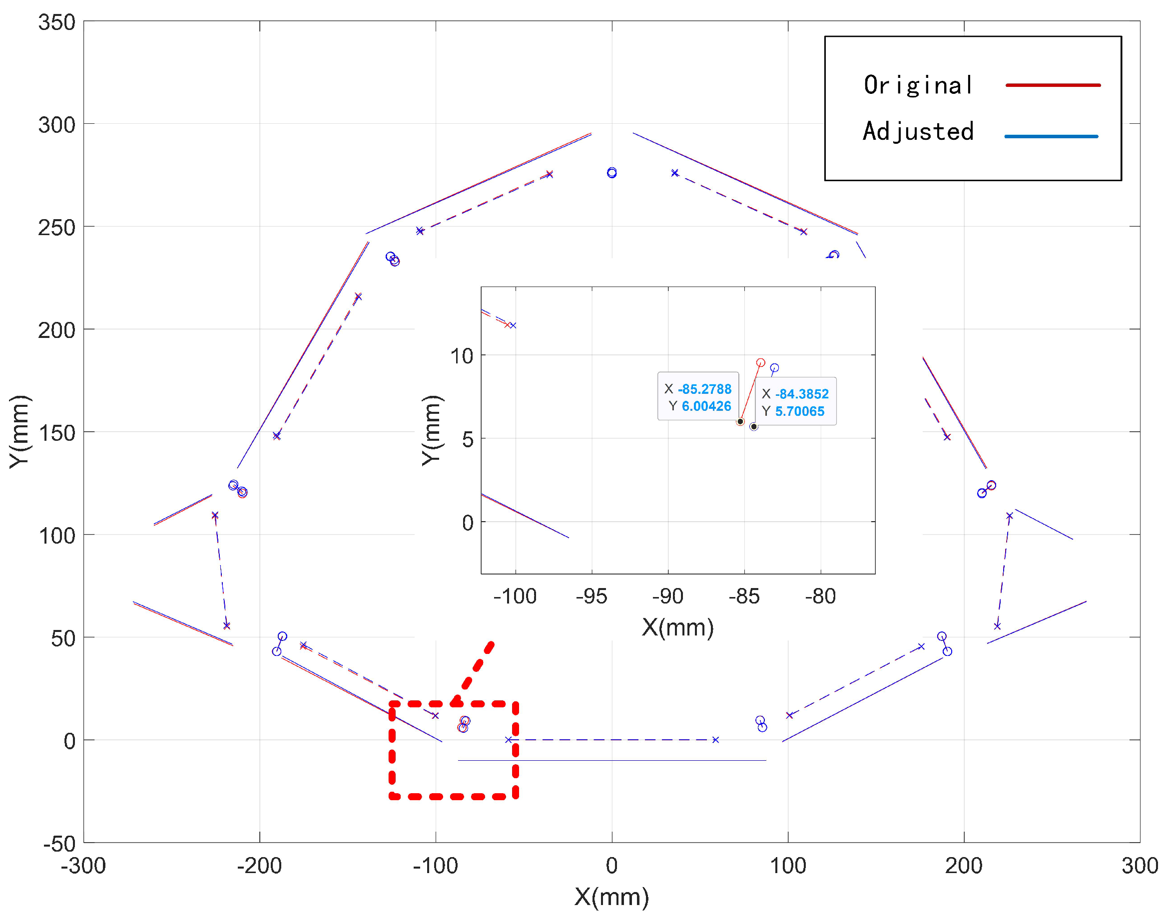
When performing assembly simulations of this structure, the key to analyzing the target parameters lies in how the geometric features are selected. According to the structural characteristics, the connection line of two feet perpendicular to the center of the reference hole to the side grinding surface is selected as one of the key geometric features to establish the vector loop. The established vector loop is shown in Figure 12.

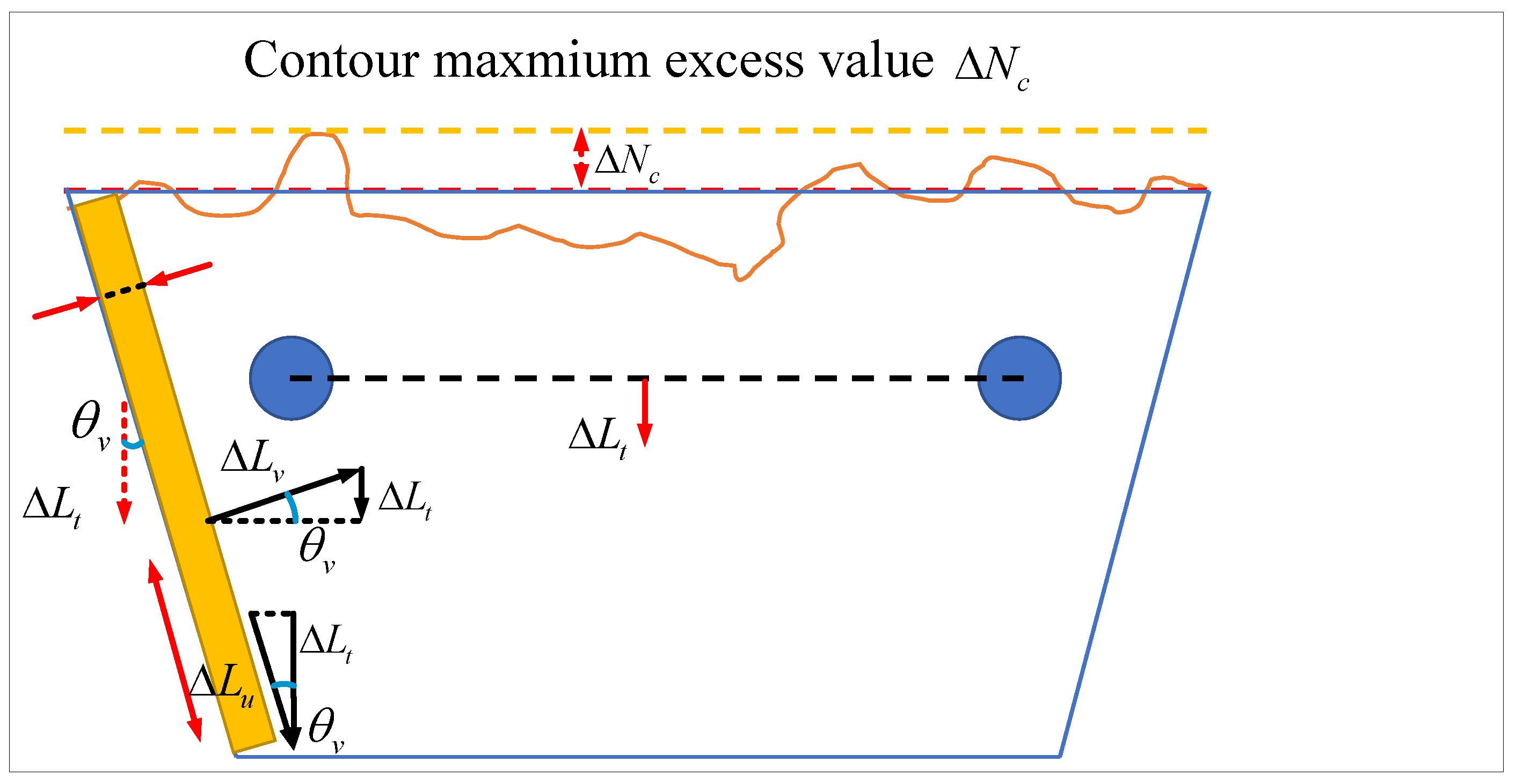
The vectors of the above-constructed vector loop include two types, IR and ARp, as shown in Figure 13. The IR vectors are determined by reference lines $L_t$, established by two reference holes; and the distance from the reference hole to the grinding surface $L_f$, the angle between reference lines and vertical line ${\theta }_f$. The ARp vectors are determined by the vector $L_a$, connecting two feet of perpendiculars on one mating surface. The angle between the normal vector on the contour and the line connecting the reference hole is represented by ${\theta }_{cn}$. The impact of the grinding amount on the mating surfaces $\Delta L_f$ to changes in the contour surfaces $\Delta N_{nc}$ (in the vertical direction of the reference hole connection line, as shown in Figure 8) of each component can be expressed by

$$\Delta N_{nc}=sin\left({\theta }_{cn}\right)\Delta L_t=sin\left({\theta }_{cn}\right)(\Delta L_{v}sin\left({\theta }_v\right)+\Delta L_{mu}cos\left({\theta }_f\right))$$

(22)

The above equation shows the relationships between the measurable value and the IR and ARp parameters in the vector loop. The nominal variables of each part are shown in

Table 1. Nominal geometric parameters of parts.

Part No.	${\mathit{L}}_{\mathit{h}}$ (mm)	${\mathit{L}}_{\mathit{fl}}$ (mm)	${\mathit{\theta }}_{\mathit{fl}}$ (°)	${\mathit{L}}_{\mathit{fr}}$ (mm)	${\mathit{\theta }}_{\mathit{fr}}$ (°)	$\mathit{min}\left({\mathit{\theta }}_{\mathit{cn}}\right)$ (°)	${\mathit{L}}_{\mathit{a}}$ (mm)
1	117.75	26.88	20.78	26.88	20.78	72.11	3.778
2	82.18	16.33	3.36	12.79	−0.85	86.41	8.072
3	54.36	30.62	59.38	17.84	42.47	16.59	6.557
4	82.91	33.69	−1.22	26.65	10.12	77.24	3.648
5	78.76	20.38	24.97	35.52	20.99	77.15	0
6	78.76	35.52	20.99	20.36	24.97	77.15	3.648
7	82.91	26.65	10.12	33.69	−1.22	77.24	6.557
8	54.36	17.84	42.47	30.62	59.38	16.59	8.072
9	82.18	12.79	−0.85	16.33	3.36	86.05	3.778

. In order to simplify the measurement in the actual calculation, the minimum angle on a contour, denoted as $min({\theta }_{cn}$), is directly incorporated into the above equation. This ensures that the contour is not exceeded after grinding, according to the calculated value.

According to the coordinate system established in Figure 12, the VLM for this structure can be expressed as

$$\begin{array}{c}\hfill \left[{\theta }_{ARp1}\right]\left[L_{ARp1}\right]\left[{\theta }_{IR1}\right]\left[L_{IR1}\right]\left[{\theta }_{ARp2}\right]\left[L_{ARp2}\right]\left[{\theta }_{IR2}\right]\left[L_{IR2}\right]\dots \left[{\theta }_{ARpi}\right]\left[L_{ARpi}\right]\left[{\theta }_{IRi}\right]\left[L_{IRi}\right]\dots \\ \hfill [{\theta }_{ARp9}]\left[L_{ARp9}\right]\left[{\theta }_{IR9}\right]\left[L_{IR9}\right]=\left[I\right]\end{array}$$

(23)

where:

• $|L_{IRi}|=L_{fli}cos(180-{\theta }_{fli})+L_{hi}+L_{fri}cos({180}^{\circ }-{\theta }_{fri})$;
• $|L_{ARpi}|=L_{ai}$;
• ${\theta }_{IRi}={90}^{\circ }+{\theta }_{f{r}_i}$ is the angle from vector $L_{IRi}$ to vector $L_{ARpi}$;
• ${\theta }_{ARpi}={90}^{\circ }+{\theta }_{fl(i+1)}$ is the angle from vector $L_{ARpi}$ to vector $L_{IR(i+1)}$.

By summing the vectors in three DOFs, which are translation in the x and y directions and rotation $\theta$, Equation (4) gives the following three equations:

$$H_x=\sum _{i=1}^9{L}_{ARpi}cos(\sum _{j=1}^i{\theta }_{ARpj}+\sum _{j=1}^{i-1}{\theta }_{IRj})+\sum _{i=1}^9{L}_{IRi}cos(\sum _{j=1}^i{\theta }_{ARpj}+\sum _{j=1}^i{\theta }_{IRj})=0$$

(24)

$$H_x=\sum _{i=1}^9{L}_{ARpi}sin(\sum _{j=1}^i{\theta }_{ARpj}+\sum _{j=1}^{i-1}{\theta }_{IRj})+\sum _{i=1}^9{L}_{IRi}sin(\sum _{j=1}^i{\theta }_{ARpj}+\sum _{j=1}^i{\theta }_{IRj})=0$$

(25)

$$H_{\theta }=\sum _{i=1}^9({\theta }_{IRi}+{\theta }_{ARp(i,i+1)})=0$$

(26)

Arranging the above equation into matrix form in Equation (7), then the matrix in the equation is represented as

$$A=\left[\begin{array}{ccccccccc}{\displaystyle \frac{\partial H_x}{\partial {\Delta }_{L_{IR1}}}}& {\displaystyle \frac{\partial H_x}{\partial {\Delta }_{L_{IR2}}}}& {\displaystyle \frac{\partial H_x}{\partial {\Delta }_{L_{IR3}}}}& {\displaystyle \frac{\partial H_x}{\partial {\Delta }_{L_{IR4}}}}& {\displaystyle \frac{\partial H_x}{\partial {\Delta }_{L_{IR5}}}}& {\displaystyle \frac{\partial H_x}{\partial {\Delta }_{L_{IR6}}}}& {\displaystyle \frac{\partial H_x}{\partial {\Delta }_{L_{IR7}}}}& {\displaystyle \frac{\partial H_x}{\partial {\Delta }_{L_{IR8}}}}& {\displaystyle \frac{\partial H_x}{\partial {\Delta }_{L_{IR9}}}}\\ {\displaystyle \frac{\partial H_y}{\partial {\Delta }_{L_{IR1}}}}& {\displaystyle \frac{\partial H_y}{\partial {\Delta }_{L_{IR2}}}}& {\displaystyle \frac{\partial H_y}{\partial {\Delta }_{L_{IR3}}}}& {\displaystyle \frac{\partial H_y}{\partial {\Delta }_{L_{IR4}}}}& {\displaystyle \frac{\partial H_y}{\partial {\Delta }_{L_{IR5}}}}& {\displaystyle \frac{\partial H_y}{\partial {\Delta }_{L_{IR6}}}}& {\displaystyle \frac{\partial H_y}{\partial {\Delta }_{L_{IR7}}}}& {\displaystyle \frac{\partial H_y}{\partial {\Delta }_{L_{IR8}}}}& {\displaystyle \frac{\partial H_y}{\partial {\Delta }_{L_{IR9}}}}\\ {\displaystyle \frac{\partial H_{\theta }}{\partial {\Delta }_{L_{IR1}}}}& {\displaystyle \frac{\partial H_{\theta }}{\partial {\Delta }_{L_{IR2}}}}& {\displaystyle \frac{\partial H_{\theta }}{\partial {\Delta }_{L_{IR3}}}}& {\displaystyle \frac{\partial H_{\theta }}{\partial {\Delta }_{L_{IR4}}}}& {\displaystyle \frac{\partial H_{\theta }}{\partial {\Delta }_{L_{IR5}}}}& {\displaystyle \frac{\partial H_{\theta }}{\partial {\Delta }_{L_{IR6}}}}& {\displaystyle \frac{\partial H_{\theta }}{\partial {\Delta }_{L_{IR7}}}}& {\displaystyle \frac{\partial H_{\theta }}{\partial {\Delta }_{L_{IR8}}}}& {\displaystyle \frac{\partial H_{\theta }}{\partial {\Delta }_{L_{IR9}}}}\end{array}\right]$$

(27)

$$B=\left[\begin{array}{ccccccccc}{\displaystyle \frac{\partial H_x}{\partial \Delta L_{ARp1}}}& {\displaystyle \frac{\partial H_x}{\partial \Delta L_{ARp2}}}& {\displaystyle \frac{\partial H_x}{\partial \Delta L_{ARp3}}}& {\displaystyle \frac{\partial H_x}{\partial {\Delta }_{LARp4}}}& {\displaystyle \frac{\partial H_x}{\partial \Delta L_{ARp5}}}& {\displaystyle \frac{\partial H_x}{\partial {\Delta }_{LARp6}}}& {\displaystyle \frac{\partial H_x}{\partial {\Delta }_{LARp7}}}& {\displaystyle \frac{\partial H_x}{\partial {\Delta }_{LARp8}}}& {\displaystyle \frac{\partial H_x}{\partial \Delta L_{ARp9}}}\\ {\displaystyle \frac{\partial H_y}{\partial \Delta L_{ARp1}}}& {\displaystyle \frac{\partial H_y}{\partial \Delta L_{ARp2}}}& {\displaystyle \frac{\partial H_y}{\partial \Delta L_{ARp3}}}& {\displaystyle \frac{\partial H_y}{\partial \Delta L_{ARp4}}}& {\displaystyle \frac{\partial H_y}{\partial \Delta L_{ARp5}}}& {\displaystyle \frac{\partial H_y}{\partial \Delta L_{ARp6}}}& {\displaystyle \frac{\partial H_y}{\partial \Delta L_{ARp7}}}& {\displaystyle \frac{\partial H_y}{\partial \Delta L_{ARp8}}}& {\displaystyle \frac{\partial H_y}{\partial \Delta L_{ARp9}}}\\ {\displaystyle \frac{\partial H_{\theta }}{\partial \Delta L_{ARp1}}}& {\displaystyle \frac{\partial H_{\theta }}{\partial \Delta L_{ARp2}}}& {\displaystyle \frac{\partial H_{\theta }}{\partial \Delta L_{ARp3}}}& {\displaystyle \frac{\partial H_{\theta }}{\partial \Delta L_{ARp4}}}& {\displaystyle \frac{\partial H_{\theta }}{\partial \Delta L_{ARp5}}}& {\displaystyle \frac{\partial H_{\theta }}{\partial \Delta L_{ARp6}}}& {\displaystyle \frac{\partial H_{\theta }}{\partial \Delta L_{ARp7}}}& {\displaystyle \frac{\partial H_{\theta }}{\partial \Delta L_{ARp8}}}& {\displaystyle \frac{\partial H_{\theta }}{\partial \Delta L_{ARp9}}}\end{array}\right]$$

(28)

$$\partial V={\left[\begin{array}{ccccccccc}{L}_{IR1}& L_{IR2}& L_{IR3}& L_{IR4}& L_{IR5}& L_{IR6}& L_{IR7}& L_{IR8}& L_{IR9}\end{array}\right]}^T$$

(29)

$$\partial U={\left[\begin{array}{ccccccccc}{L}_{ARp1}& L_{ARp2}& L_{ARp3}& L_{ARp4}& L_{ARp5}& L_{ARp6}& L_{ARp7}& L_{ARp8}& L_{ARp9}\end{array}\right]}^T$$

(30)

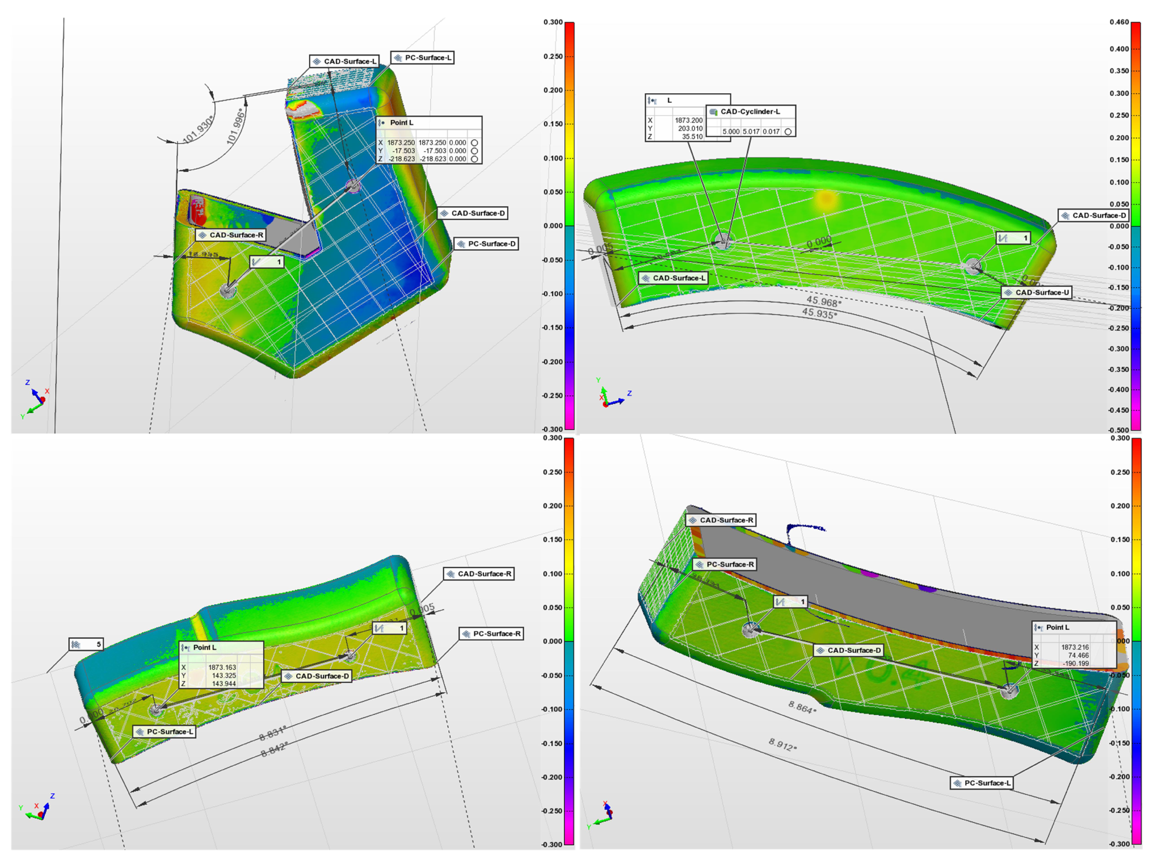
Then, the SMS of each part is generated based on the measured data, as is shown in Figure 14. And the deviation of each geometric parameter and contour are obtained through the SMS, and the assembly deviation of each assembly mating surface is obtained through the SMS and the contact state analysis method, as shown in

Table 2. Geometric deviations of parts.

Part No.	$\mathbf{\Delta }{\mathit{L}}_{\mathit{h}}$ (mm)	$\mathbf{\Delta }{\mathit{L}}_{\mathit{fl}}$ (mm)	$\mathbf{\Delta }{\mathit{\theta }}_{\mathit{rpl}}$ (°)	$\mathbf{\Delta }{\mathit{L}}_{\mathit{fr}}$ (mm)	$\mathbf{\Delta }{\mathit{\theta }}_{\mathit{rpr}}$ (°)	$\mathbf{\Delta }{\mathit{N}}_{\mathit{nc},\mathit{max}}$
1	−0.031	0.081	−0.012	0.069	0.006	0.065
2	−0.251	0.23	−0.009	−0.201	−0.046	0.003
3	0.029	0.333	−0.024	0.283	−0.149	0.006
4	−0.014	0.159	0.043	−0.052	0.038	0.035
5	−0.021	−0.001	0.019	0.167	−0.063	0.07
6	0.09	−0.007	0.009	0.023	−0.024	0.07
7	−0.908	0.083	0.043	−0.223	−0.093	0.04
8	0.003	0.303	−0.023	0.557	−0.167	0.02
9	0.518	−0.361	0.004	0.574	0.36	0.025

.

The maximum allowable excess value (unit in mm) of each contour is set as below, on the basis of assembly requirements for corresponding structures of aerospace vehicles.

$$Max\left(N_c\right)=[0.6,0.6,0.6,0.6,0.6,0.6,0.6,0.6,0.6]$$

(31)

Combined with the measured data in Table 2, the need for grinding is analyzed based on the model expressed in Equations (7) and (27)–(30) and the criterion proposed in Section 3.3. The closed-loop excess values are analyzed based on the objective function method, and the “fmincon” function in MATLAB is used for practical calculations. The calculated results indicate that the closed loop of the vector loop is interfering, with a value of 0.883 mm, as shown in Figure 15, and therefore, further grinding on mating surfaces is required.

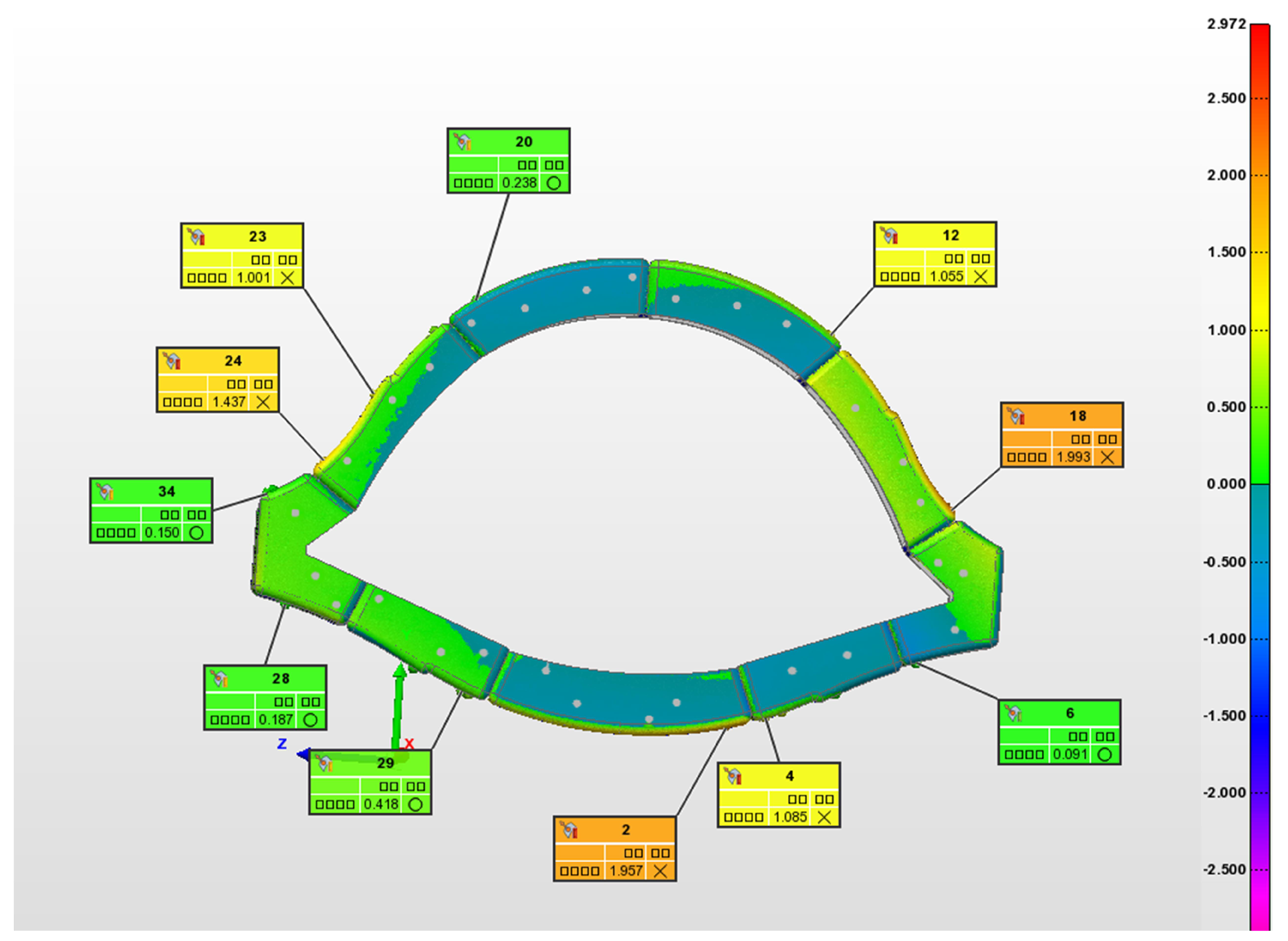
Three assemblies and measurements are carried out by directly assembling the parts that have not been ground. The measured contours of the assembly are shown in Figure 16 and

Table 3. Contour error of original parts in each assembly.

Part No.	1	2	3	4	5	6	7	8	9
Assembly No.	Contour Excess Value (mm)
1	1.957	1.085	0.091	1.993	1.055	0.238	1.437	0.187	0.418
2	2.131	0.434	0.368	2.201	1.117	1.089	1.153	0.165	0.217
3	1.269	1.291	0.398	1.010	0.197	0.179	1.231	0.392	0.106

. The results indicate that a qualified assembly could not be completed without grinding and repairing the mating surfaces, which is consistent with the algorithm’s prediction. The contour excess rate of the assembled body parts is 51.9%, and the average value of the contour excess value is 0.867 mm.

The maximum allowable grinding amounts (unit in mm) of each grinding surface were set as below, on the basis of grinding requirements for corresponding structures of aerospace vehicles.

$$Max(\Delta L_{IR})=[0.4,0.4,0.4,0.4,0.4,0.4,0.4,0.4,0.4]$$

(32)

By combining Equations (12), (27) and (28), the relationship between the grinding amount $\Delta L_v$ and the closed-loop deviation $\Delta L_{IR9}$, represented by the sensitive matrix $\left[S\right]$, can be calculated. Along with the calculated deviation values in the closed loop and the grinding amount limitation, the sensitive matrix and the grinding solution are presented in

Table 4. Sensitivity factor of each grinding amount $\Delta L_{IR}$ to closed-loop deviation $\Delta L_{IR9}$.

Part No.	Sensitivity Factor	Grinding Amount
$\Delta L_{IR1}$	0.7454	0.113
$\Delta L_{IR2}$	0.7162	0
$\Delta L_{IR3}$	−0.5724	0
$\Delta L_{IR4}$	−0.9045	0
$\Delta L_{IR5}$	−0.9356	0
$\Delta L_{IR6}$	−0.3969	0
$\Delta L_{IR7}$	−0.2509	0
$\Delta L_{IR8}$	0.9987	0.4
$\Delta L_{IR9}$	1	0.4

.

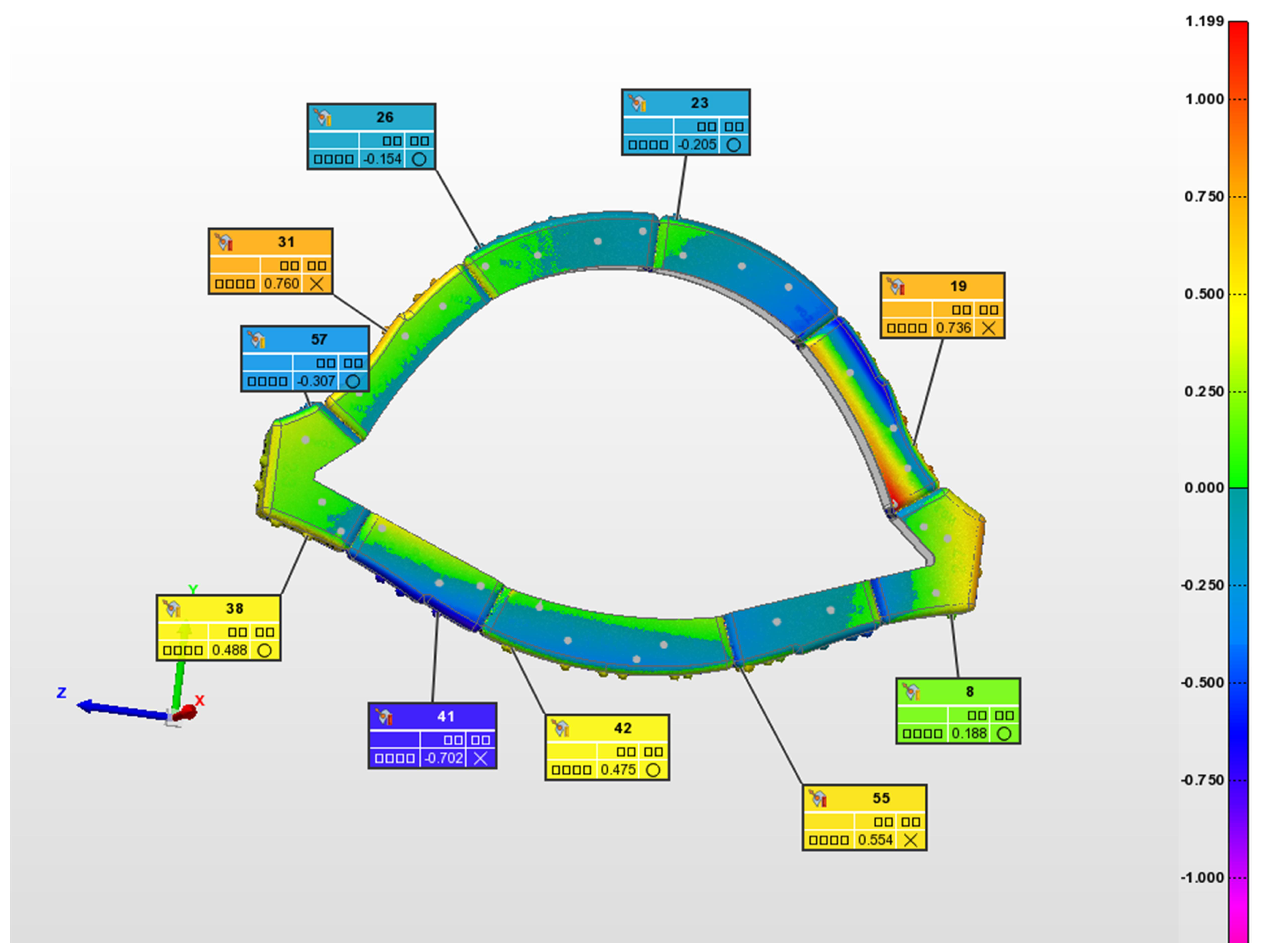
According to the algorithm’s analysis results, the parts were ground, and then, assembled. Three assemblies and measurements were carried out, and the results are shown in Figure 17 and

Table 5. Contour error of ground parts in each assembly.

Part No.	1	2	3	4	5	6	7	8	9
Assembly No.	Contour Excess Value (mm)
1	0.855	0.135	0.322	0.353	0.573	0.5	0.832	0.09	0.523
2	0.475	0.055	0.188	0.736	−0.295	−0.154	0.76	0.488	−0.702
3	0.49	0.598	0.157	0.443	0.218	0.338	0.452	0.495	−1.191

.

The results show that after grinding the contour excess rate is reduced to 14.8% and the average value of contour excess is reduced to 0.286 mm. Some values still exceed the allowed range after the adjustment. It is presumed that the lack of assembly precision in the laboratory environment has led to the matching surfaces not being fully adhered, leading to inaccurate adjustments of the assembly relationship $\Delta L_u$ and the grinding value $\Delta L_v$. In order to solve this problem, it is planned to determine an adjustment correction factor through more assembly tests in future work.

5. Conclusions

This work proposes a data-driven assembly geometric precision analysis and optimization method for underconstrained structures. The main contributions are as follows:

• A VLM-SMS modeling method is proposed. Dimensional features and dimensional deviation transfer paths of the target structure are described by the VLM. The SMS method is employed to describe the surface morphology deviation of the part’s surface and analyze its influence on the assembly accuracy of the mating surfaces.
• An assembly-stage-oriented optimization method for underconstrained structures is proposed. By considering the actual process, additional constraints are established to facilitate the analysis. This method determines whether a group of parts needs to be ground through the objective function, then allocates the amount of grinding through sensitivity analysis to improve assembly efficiency by reducing the number of grinding surfaces.
• The effectiveness of the proposed method is verified through assembly experiments. The experiment results show that under the guidance of the proposed method, there is a significant improvement in the contour excess rate and average contour excess value of the assembly after grinding.

However, there are still shortcomings in the existing methods: (1) After grinding and repairing according to the guidance of the proposed methodology, some excess deviations still exist. It is hypothesized that this is due to the insufficiency of the existing assembly tools, resulting in the precision of the adjustment amount not being accurate. (2) There might be a situation where the mating surfaces are not fully adherent, which introduces a rotational deviation. (3) The proposed method can only optimize structure in series connections. However, in the case of real products, where structures with parallel connections exist, the proposed method is not applicable. Deformations due to internal stresses are also omitted in these assembly scenarios, while in some assembly scenarios deformations cannot be ignored. Future work will consider the impact of rotational errors introduced by mating surface misalignment on assembly, and determine a set of adjustment correction factors through more assembly tests; data analysis methods will also be applied to find potential data correlations based on measurement data. Simultaneously, efforts will be directed towards developing high-precision assembly tooling applicable for more complex structures. Supplementary optimization algorithms suitable for parallel structures, as well as algorithms that can take deformation into account, will be explored in future work.

References

1. Man, Y.; Han, J.; Jiang, L.; Chen, B.; Luo, M. Research an Implementation of Layout Rapid Design System for Aerospace Vehicle. Comput. Meas. Control 2020, 28, 182–187. [Google Scholar]
2. Lei, D.; Li, Y.; Xu, Y. Conceptual Design and Aerodynamic Shape Optimization for the Assembled Air Launched Vechicles Based on the BWB Carrier Aircraft. Phys. Gases 2022, 7, 50–62. [Google Scholar]
3. Yang, Z.; Zhang, D.; Gu, C. Research and application of advanced resin matrix composites for aerospace shuttle vehicles abroad. Acta Mater. Compos. Sin. 2022, 39, 3029–3043. [Google Scholar]
4. Yang, Y. Research on 3D Tolerance Simulation Analysis of Aircraft Composite Structure Assembly Based on Multiple Key Characteristics. Master’s Thesis, Zhejiang University, Hangzhou, China, 2022. [Google Scholar]
5. Hao, L.; Liu, H.; Huang, X.; Li, L.; Xie, Y.; Liu, C.; Song, J.; Yu, L.; Hou, G. Review of virtual pre-assembly technology for aircraft based on measured data. Aeronaut. Manuf. Technol. 2024, 67, 65–77. [Google Scholar]
6. Zhang, S.; Liu, X.; Zhang, C.; Wu, H.; Li, F.; Zhang, B. Tolerance Analysis and Research of Aircraft Wing Assembly Process Based on 3DCS. Aeronaut. Manuf. Technol. 2021, 1, 73–78. [Google Scholar]
7. Wang, H. Advanced Composite Part Assembly: A Survey of Methodologies and Practices. Aeronaut. Manuf. Technol. 2018, 61, 26–33. [Google Scholar]
8. Dong, Z.; Wang, Z.; Ran, Y.; Bao, Y.; Kang, R. Advances in Ultrasonic Vibration-Assisted Milling of Carbon Fiber Reinforced Ceramic Matrix Composites. J. Mech. Eng. 2023, 59, 1–31. [Google Scholar]
9. Desrochers, A.; Rivière, A. A matrix approach to the representation of tolerance zones and clearances. Int. J. Adv. Manuf. Technol. 1997, 125, 14–22. [Google Scholar]
10. Desrochers, A. A CAD/CAM representation model applied to tolerance transfer methods. J. Mech. Des. 2003, 13, 630–636. [Google Scholar]
11. Chase, K. Tolerance analysis of 2-d and 3-d assemblies. ADCATS Rep. 2004, 94, 17–25. [Google Scholar]
12. Chase, K.; Gao, J.; Magleby, S. General 2-D Tolerance Analysis of Mechanical Assemblies with Small Kinematic Adjustments. J. Des. Manuf. 1995, 5, 263–274. [Google Scholar]
13. Laperrière, L.; Ghie, W.; Desrochers, A. Statistical and Deterministic Tolerance Analysis and Synthesis Using a Unified Jacobian-Torsor Model. J. Des. Manuf. 2002, 51, 417–420. [Google Scholar]
14. Lafond, P.; Laperrière, L. Jacobian-based modeling of dispersions affecting pre-defined functional requirements of mechanical assemblies. In Proceedings of the 1999 IEEE International Symposium on Assembly and Task Planning (ISATP’99) (Cat. No. 99TH8470), Porto, Portugal, 24 July 1999. [Google Scholar]
15. Bourdet, P. The concept of small displacement torsor in metrology. Ser. Adv. Math. Appl. Sci. 1996, 40, 110–122. [Google Scholar]
16. Mujezinovic, A.; Davidson, J.; Shah, J. A New Mathematical Model for Geometric Tolerances as Applied to Polygonal Faces. J. Mech. Des. 2001, 126, 504–518. [Google Scholar]
17. Liu, Y. Hierachical representation model and its realization of tolerance based on feature. Chin. J. Mech. Eng. 2003, 39, 649–650. [Google Scholar]
18. Jiang, K.; Davidson, J.; Shah, J.; Liu, J. Using tolerance-maps to transfer datum plane from design tolerancing to machining tolerancing. In Proceedings of the International Design Engineering Technical Conferences and Computers and Information in Engineering Conference, Portland, OR, USA, 4–7 August 2013; V004T05A023. [Google Scholar]
19. Yan, X.; Ballu, A. Tolerance analysis using skin model shapes and linear complementarity conditions. J. Manuf. Syst. 2018, 48, 140–156. [Google Scholar]
20. Schleich, B.; Anwer, N.; Mathieu, L.; Wartzack, S. Skin Model Shapes: A new paradigm shift for geometric variations modelling in mechanical engineering. Comput.-Aided Des. 2014, 50, 1–15. [Google Scholar]
21. Sun, Q.; Zhao, B.; Liu, X.; Mu, X.; Zhang, Y. Assembling deviation estimation based on the real mating status of assembly. Comput.-Aided Des. 2019, 115, 244–255. [Google Scholar]
22. Liu, J.; Zhang, Z.; Ding, X.; Shao, N. Integrating form errors and local surface deformations into tolerance analysis based on skin model shapes and a boundary element method. Comput.-Aided Des. 2018, 104, 45–59. [Google Scholar]
23. Gao, J.; Chase, K.; Magleby, S. General 3-D tolerance analysis of mechanical assemblies with small kinematic adjustments. J. Des. Manuf. 1998, 30, 367–377. [Google Scholar]
24. Li, J.; Zhao, G.; Zhang, P. A Digital Twin-based on-site quality assessment method for aero-engine assembly. J. Manuf. Syst. 2023, 71, 565–580. [Google Scholar]
25. Liu, T. Study on the Methods of Assembly Error Analysis Based on Skin Model Shapes. Ph.D. Thesis, Zhejiang University, Hangzhou, China, 2019. [Google Scholar]
26. Hultman, H.; Cedergren, S.; Warmefjord, K.; Söderberg, R. Predicting Geometrical Variation in Fabricated Assemblies Using a Digital Twin Approach Including a Novel Non-Nominal Welding Simulation. Aerospace 2022, 9, 512. [Google Scholar] [CrossRef]
27. Bao, Q.; Zhao, G.; Yu, Y.; Dai, S.; Wang, W. Ontology-based modeling of part digital twin oriented to assembly. Proc. Inst. Mech. Eng. Part B J. Eng. Manuf. 2022, 236, 16–28. [Google Scholar]
28. Ye, Y.; Fan, G.; Ou, S. An algorithm for judging points inside or outside a polygon. In Proceedings of the 2013 Seventh International Conference on Image and Graphics, Qingdao, China, 26–28 July 2013; IEEE: Piscataway, NJ, USA, 2013; pp. 690–693. [Google Scholar]
Figure 1. An example of vector loop and component vectors.
Aerospace 11 00689 g001
Figure 2. Difference between the nominal model, the skin model, and the physical part [20].
Aerospace 11 00689 g002
Figure 3. Assembly-stage-oriented SMS modeling method.
Aerospace 11 00689 g003
Figure 4. Implementation steps of the SMS-VLM methodology.
Aerospace 11 00689 g004
Figure 5. Typical structure of aerospace vehicle.
Aerospace 11 00689 g005
Figure 6. Assembly mating surface deviation forms.
Aerospace 11 00689 g006
Figure 7. Mapping between assembly features and information models.
Aerospace 11 00689 g007
Figure 8. Relationships between assembly mating surface deviation and grinding amount.
Aerospace 11 00689 g008
Figure 9. Determined assembly sequence (From Part 1 to Part 9) of the structure.
Aerospace 11 00689 g009
Figure 10. Excess condition of the final mating surface.
Aerospace 11 00689 g010
Figure 11. Assembly test parts.
Aerospace 11 00689 g011
Figure 12. Vector loop of assembly test parts.
Aerospace 11 00689 g012
Figure 13. Components of vector IRs and ARps.
Aerospace 11 00689 g013
Figure 14. Parts’ SMSs built based on measured data.
Aerospace 11 00689 g014
Figure 15. Calculations based on measured data under constraints.
Aerospace 11 00689 g015
Figure 16. An assembly contour error before grinding. × indicates that the contour surface error is not qualified, and ∘ indicates that the contour surface error is qualified.
Aerospace 11 00689 g016
Figure 17. An assembly contour error after grinding. × indicates that the contour surface error is not qualified, and ∘ indicates that the contour surface error is qualified.
Aerospace 11 00689 g017