Article

Mars Exploration: Research on Goal-Driven Hierarchical DQN Autonomous Scene Exploration Algorithm

1
School of Integrated Circuits and Electronics, Beijing Institute of Technology, Beijing 100081, China
2
Faculty of Data Science, City University of Macau, Macau, China
*
Authors to whom correspondence should be addressed.
Aerospace 2024, 11(8), 692; https://doi.org/10.3390/aerospace11080692
Submission received: 22 July 2024 / Revised: 16 August 2024 / Accepted: 20 August 2024 / Published: 22 August 2024
(This article belongs to the Section Astronautics & Space Science)

Abstract

:
In the non-deterministic, large-scale navigation environment under the Mars exploration mission, there is a large space for action and many environmental states. Traditional reinforcement learning algorithms that can only obtain rewards at target points and obstacles will encounter the problems of reward sparsity and dimension explosion, making the training speed too slow or even impossible. This work proposes a deep layered learning algorithm based on the goal-driven layered deep Q-network (GDH-DQN), which is more suitable for mobile robots to explore, navigate, and avoid obstacles without a map. The algorithm model is designed in two layers. The lower layer provides behavioral strategies to achieve short-term goals, and the upper layer provides selection strategies for multiple short-term goals. Use known position nodes as short-term goals to guide the mobile robot forward and achieve long-term obstacle avoidance goals. Hierarchical execution not only simplifies tasks but also effectively solves the problems of reward sparsity and dimensionality explosion. In addition, each layer of the algorithm integrates a Hindsight Experience Replay mechanism to improve performance, make full use of the goal-driven function of the node, and effectively avoid the possibility of misleading the agent by complex processes and reward function design blind spots. The agent adjusts the number of model layers according to the number of short-term goals, further improving the efficiency and adaptability of the algorithm. Experimental results show that, compared with the hierarchical DQN method, the navigation success rate of the GDH-DQN algorithm is significantly improved, and it is more suitable for unknown scenarios such as Mars exploration.

1. Introduction

Planetary surface exploration is a significant branch in the field of deep space exploration [1]. To gain a better understanding of an extraterrestrial body, the most effective approach is to land on its surface and conduct reconnaissance and exploration [2,3]. Currently, the main countries involved in the development of planetary surface rovers are the United States, the European Space Agency (ESA), and China [4]. The National Aeronautics and Space Administration (NASA) Mars 2020 Perseverance Rover and Ingenuity helicopter landed in the Jezero Crater in February 2021 [5]. China’s Mars rover, Zhurong, touched down on Utopia Planitia in the northern lowlands of Mars in May 2021 [6]. In the field of Mars exploration simulator research, the National Aeronautics and Space Administration (NASA) has developed a Mars exploration game to simulate the exploration of the Martian terrain and the completion of tasks such as searching for water sources. The European Mars Probe Challenge in Poland began in 2014 with the establishment of a live simulation field. Harbin Institute of Technology in China has also built a simulation environment for Martian landscapes, considering irregular contact areas and simulating phenomena such as wheel slippage [7].
Planetary surface rovers are highly integrated, compact, and intelligent semi-autonomous or fully autonomous mobile robots designed for exploring planetary surfaces [8]. These rovers autonomously navigate and explore planetary terrains, often requiring them to complete navigation and obstacle avoidance tasks between multiple waypoints and ultimately reach their destination [9]. Faced with unpredictable and unknown environments, mobile robots not only need to reach specified locations but also need to intelligently plan efficient paths, avoid obstacles, successfully reach each waypoint, and accomplish their respective tasks [10]. Conventional navigation methods, such as the A* algorithm [11] and the artificial potential field technique [12], require accurate map data of the surrounding area to ensure safe and efficient planning. However, the current Mars probe lacks terrain information and needs to travel without more frequent communications between Earth and Mars [13]. To elucidate, any malfunction of the sensors or delays in data processing will significantly impede the subsequent execution of the path planning algorithm. This segmented robot planning method has low intelligence and cannot deal with complex environments. The low efficiency of path-planning algorithms in complex environments with dense obstacles has become one of the main factors hindering the development of robotic rovers [14].
Reinforcement learning stands as a computational approach employed to understand and automate the process of goal-driven learning and decision-making [15]. Within this framework, reinforcement learning techniques acquire suitable actions based on the prevailing environmental state. As the agent interacts with the external environment, it integrates the reward signal through exploratory actions and iterative trial-and-error learning. This amalgamation of processes allows the agent to gather environmental insights and iteratively refine its navigation strategy [16]. To further enhance the ability of reinforcement learning to perceive the environment, Google’s DeepMind team proposed a deep reinforcement learning (DRL) algorithm for the first time [17], which combined deep learning and reinforcement learning to understand high-dimensional input and make intelligent decisions using information. DRL enables robots to sense the environment, such as humans, in the absence of accurate maps and to efficiently complete navigation tasks by interacting with the environment and learning. The popularity of DRL has enabled smarter robots to navigate and avoid obstacles, which could potentially be used to enable autonomous navigation for Mars rovers.
The main contributions of this work can be itemized as follows:
  • Addressing the current dependency of Mars rover motion control on ground-based remote operations, this study proposes a reinforcement learning method called GDH-DQN to enable the Mars rover to have autonomous movement and path planning capabilities.
  • Given the vast scale of the Martian environment, the lack of prior maps, and the prevalence of numerous, densely packed, and irregularly-shaped obstacles, our GDH-DQN method effectively addresses the challenges of sparse rewards and the explosion of state dimensions in large-scale Mars exploration scenarios.
  • Integrating the hindsight experience replay mechanism into the hierarchical reinforcement learning algorithm eliminates the need for complex reward function design, fully harnessing the intrinsic potential of the data, enhancing sample efficiency, and expediting model convergence. We conducted extensive training and testing experiments, demonstrating the high performance and robust adaptability of the GDH-DQN method in large-scale planet exploration scenarios.

2. Related Works

2.1. Deep-Reinforcement-Learning-Based Navigation Methods

Deep reinforcement learning (DRL) has made great progress in recent years and has become a key area of artificial intelligence research. By integrating the advantages of deep learning and reinforcement learning, the DRL algorithm can learn effective strategies in high-dimensional and complex environments. In 2013, DeepMind [18] proposed the Deep Q Network (DQN), demonstrating the potential of DRL to solve complex tasks and marking the beginning of a new era of deep reinforcement learning research. In 2016, DeepMind [19] launched the Asynchronous Advantage Actor-Critic (A3C) algorithm, which improves the efficiency and stability of training by exploiting asynchronous parallelism. In 2017, OpenAI [20] introduced the Proximal Policy Optimization (PPO) algorithm, which has since become one of the most widely used methods in deep reinforcement learning due to its simplicity, robustness, and performance.
However, there are still some challenges in applying deep reinforcement learning to Mars rover navigation. There are two main problems: on the one hand, the mechanism where agents receive positive rewards only upon reaching the goal point leads to the sparse reward problem. On the other hand, due to the independent exploration scene, the algorithm has a dimension explosion in the training process. These two problems increase the difficulty of DRL training, and it is difficult to agree on the optimal strategy.
In reinforcement learning, rewards guide the learning direction of the agent [21,22], and the lack of reward information will lead to the slow learning progress of the agent or even the inability to learn the optimal strategy, which is the sparse reward problem [23]. In the navigation environment, rewards and experiences are generated solely when the agent reaches obstacles or target points. At other times, rewards are zero, impacting the ability of DRL to gather sufficient useful experience, thus affecting algorithm performance. Approaches to address the challenge of sparse rewards encompass reward shaping [24], the hindsight experience replay mechanism (HER) [25], as well as hierarchical reinforcement learning, among others.
Reward shaping is a prevalent technique. It involves the incorporation of prior knowledge to construct an augmented reward function that steers the agent toward accomplishing the intended task. Jagodnik et al. [26] used distance information calculation and subjective evaluation as the reward function to control the manipulator, and the effect was better than that of the optimized proportional differential controller. Brito et al. [27] used deep reinforcement learning to recommend sub-goals for model predictive control, in which the Euclidean distance to the target point was used as a reward to accelerate learning.
However, reward shaping is limited and often benefits from a well-designed reward function, which requires a large amount of prior knowledge in the corresponding field and has poor generalization. For obstacle avoidance tasks, the commonly used Euclidean distance will mislead the agent, and it is difficult for the agent to deal with complex environments such as dead corners and corridors [28,29], which makes it difficult for the algorithm to be applied to environments with high requirements for dynamic confrontation and real-time decision-making. Different from reward shaping, the hindsight experience replay [30] mechanism adds the input information of the goal and generates the successful sample by correcting the goal of the failed sample generated in the learning process so that the agent can obtain the positive reward faster, greatly improving the algorithm training efficiency. Moreover, it reduces susceptibility to the complexity of obstacle-laden environments and proves adaptable to scenarios involving multi-goal learning.
Although deep reinforcement learning has achieved good results in no-map navigation, the data efficiency of deep reinforcement learning is low, and it is very sensitive to environmental disturbance. Therefore, navigation based on deep reinforcement learning is mostly limited to small-range scenarios.

2.2. Mars Rover Navigation Methods

The Opportunity and Curiosity rovers possess only 5% of their potential autonomous navigation distance, with minimal autonomous navigation capability. Although the Perseverance rover is equipped with an automatic navigation system [31], its maximum autonomous navigation distance is less than 700 m [32]. This indicates that current Mars rover missions have not achieved fully autonomous navigation and remain heavily reliant on human remote operation [33]. The vast distance between Earth and Mars, combined with the limited computing resources of the Mars rovers, imposes significant constraints on human remote operation and control. These constraints include the infrequent issuance of remote commands, typically only once every 1 to 3 days; the limited operational time available for the rovers, usually around 3 h of driving per Martian day; and the restricted processing power due to the low CPU clock frequency of the radiation-hardened processor boards used. Overall, reducing the dependence of Mars navigation missions on human intervention remains a significant challenge. Future Mars exploration missions necessitate the development of truly autonomous rover systems capable of effective navigation, along with intelligent methods tailored for systems with limited resources [32].
Since the surface of the planet is covered with unknown, uncertain, and discontinuous craters, ravines, and sandy areas, as shown in Figure 1 [34], the environmental range is large, and the conditions are diverse [35]. Therefore, the performance of the algorithm will plummet due to problems such as dimension explosions [36]. Faust et al. [37] combined probabilistic road maps with RL. Probabilistic road maps divided a large flat map into several small local maps and then used RL to learn local map navigation and obtain a map with only signpost points. The final deployment only needs to find the shortest path in the case of a given goal and then go one by one through the landmark point and reach the target point. This method effectively solves the problem of long-distance navigation, but it still needs to obtain the plan in advance and can only be navigated on the trained map at a time.
Hierarchical reinforcement learning can solve the original problem by dividing the complex problem into several small problems and solving the small problems separately. Hierarchical reinforcement learning can effectively solve the dimension explosion problem of reinforcement learning by studying how to abstract complexity into different levels and using hierarchical structure to learn strategies at different levels to better solve the problem [38,39]. Its essence is to decompose the task into sub-tasks at different levels of abstraction; the low level provides the optimal strategy for completing the sub-tasks, and the upper level provides the appropriate sub-tasks for the low level to obtain the optimal strategy for solving the overall task. At the same time, the hierarchical deep reinforcement learning method further solves the sparse reward problem by reducing the action sequence space of each layer strategy.
Hierarchical reinforcement learning includes two methods based on options and subgoals. In the option-based approach, the upper level is responsible for selecting from the low-level policy, and then the low-level policy outputs the control action. Lu et al. [40] solved the horizontal and vertical motion planning problem at the low planning level, while the upper level simulated and evaluated various scenarios, therefore completing the optimization decision in the complex traffic environment. The subgoal-based method generates subgoals through high-level policies and completes subgoals through low-level policies. Naveed et al. [41] proposed a kind of robust hierarchical reinforcement learning in which the upper level is used for maneuver decision-making and the low level is used for waypoint trajectory generation, which solves the trajectory safety problem of automatic driving.
Although hierarchical reinforcement learning can solve the dimensional explosion problem in long-distance navigation, its ability to cope with complex environments depends on the single-layer goal completion strategy, so it is necessary to optimize the model of each layer while adopting the hierarchical framework. Robert et al. [42] proposed planning-reinforcement hierarchical reinforcement learning (PAHRL), which extracted multiple subtasks from the original problem and performed navigation tasks from one state to another in the subtasks. The feasibility of this hierarchical idea was verified on a robotic arm. Jan et al. [43] proposed a new framework that combined the plan in the high-level state space with the subgoals in the original continuous state space and introduced the value-iteration-based planning strategy. Even if the low-level strategy failed to achieve the subgoals, it could still maintain good performance in the complex terrain environment by adjusting the high-level model using the collected data.
The current Mars rover still uses traditional signal transmission to control movement and has not yet applied reinforcement-learning navigation strategies. This work attempts to apply a hierarchical reinforcement learning navigation algorithm to the autonomous navigation system of Mars probes. Due to the large scope of the Mars exploration mission, the large and dense obstacles, and the lack of prior map information, the reinforcement learning mechanism faces challenges such as sparse rewards and dimensional explosion. To address these issues, which can lead to difficulties in algorithm convergence, this paper proposes a hierarchical deep reinforcement learning algorithm, GDH-DQN, based on goal drive for the no-map obstacle avoidance of robots. In this method, a two-layer structure is adopted. A single-goal-driven model is designed at the low level to provide the behavior strategy, and a multi-goal selection strategy is provided at the upper level. The hindsight experience replay mechanism is used in each layer to improve the performance of the algorithm, which effectively avoids the possibility of misleading the agent in the complex process of designing the reward function and the complex environment, such as dead corners. In addition, the method can select the number of model layers according to the size of the environment and the number of targets, give full play to the role of each layer model, and improve the obstacle avoidance efficiency.

3. Principles of Algorithms

The Mars surface exploration mission has a large scope and no prior environmental information. To address the issue of sparse rewards during navigation in unknown environments and the convergence difficulties caused by dimension explosion in long-distance navigation with DRL, we constructed a two-layered obstacle avoidance framework based on goal-driven methods. In this framework, the high-level policy responsible for achieving the overall goal provides the suggested goal for the low-level policy, and the low-level policy is responsible for planning the reasonable path for the agent to reach the goal provided by the high-level policy. This method effectively solves the sparse reward problem and simplifies the exploration process by using the hierarchical strategy of goals to decompose complex tasks into multiple subtasks. The high-level policy solely necessitates identifying the accurate succession of goals, whereas the low-level policy is simplified to achieve the designated objective.
Considering the complex structures such as rock fissures and dead zones that exist in the Martian environment and the fact that the design reward function is not generalized, we employ a hindsight experience replay mechanism as a form of reward. The high-level policy, tasked with accomplishing the overarching objective, receives sparse environmental rewards aligned with that specific goal. Furthermore, it obtains a slight positive reward for each achieved sub-goal attained through the selection of lower-level strategies. To enhance this, a minor penalty is applied when a previously attained waypoint is chosen, deterring the strategy from becoming ensnared in local minima originating from the initial position.

3.1. Reinforcement Learning Theoretical Framework

The algorithmic principle of reinforcement learning is grounded in the concept of an agent learning an optimal policy through experimentation and feedback within an environment. At each state, the agent selects an action and updates its strategy based on feedback from the environment, which usually consists of rewards or penalties. The agent’s goal is to optimize its actions to maximize the long-term cumulative rewards from the starting point to the target point while avoiding obstacles. Through continuous interaction with the environment, the agent gradually learns the most effective actions to take in different states, thus achieving successful path planning to reach the target point.
Research has shown that Markov Decision Processes (MDP) can effectively address most reinforcement learning problems and have thus become the foundational framework for reinforcement learning theory [44]. MDP abstracts the reinforcement learning problem as a quintuple ( S , A , P , R , γ ) [45], where:
  • State space S: Represents all possible states of the environment.
  • Action space A: Represents all possible actions that the agent can take in each state.
  • State transition probability P (s′|s, a): Describes the probability of transitioning to the next state s′ after taking action a in state s.
  • Reward function R (s, a): The immediate reward received by the agent for taking action a in state s. Reflects the agent’s progress toward its goal.
  • Discount factor γ : Balances the importance of current and future rewards, with values between 0 and 1.
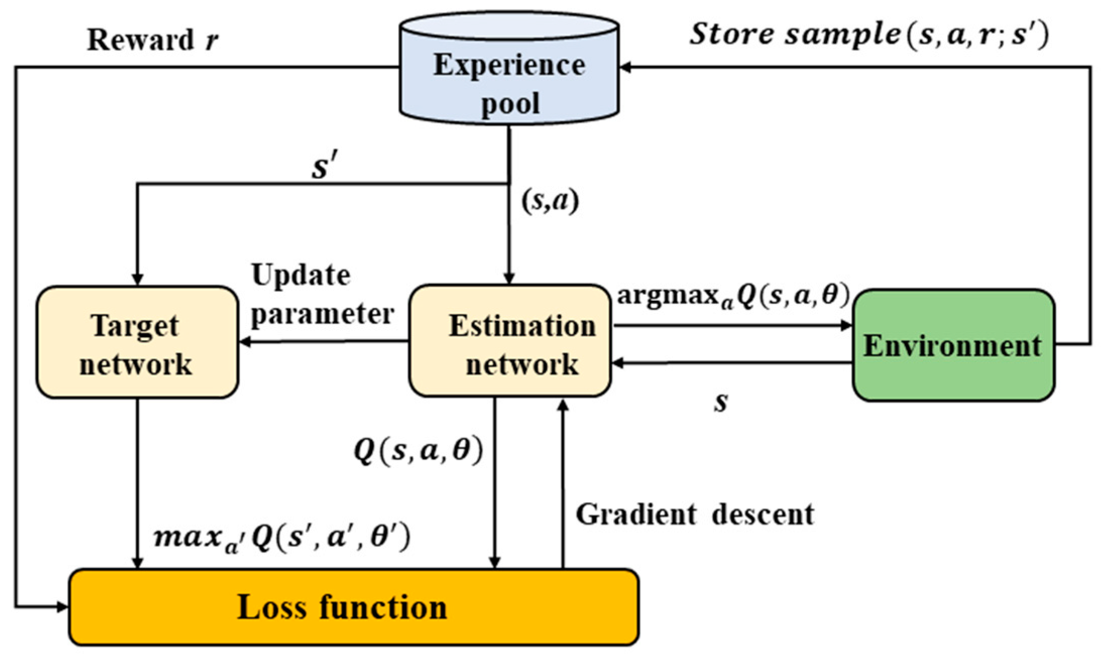
The agent’s goal is to find the optimal policy π * ( a | s ) , which is a rule for selecting actions in each state s that maximizes the expected cumulative future rewards. This can be described using the state value function V π ( s ) and the state-action value function Q π ( s , a ) :
State value function  V π ( s ) is defined as the expected cumulative reward when following policy π starting from state s:
V π ( s ) = E π [ t = 0 γ t R ( s t , a t ) | s 0 = s ]
State-action value function  Q π ( s , a ) represents the expected cumulative reward when taking action aaa in state sss and then following policy π :
Q π ( s , a ) = E π [ t = 0 γ t R ( s t , a t ) | s 0 = s , a 0 = a ]
The Bellman equation for the state value function is given by:
V π ( s ) = a A π ( a | s ) s S P ( s | s , a ) [ R ( s , a ) + γ V π ( s ) ]
Through the recursive computation of state and action values, the Bellman equation enables the agent to assess the relative merits of different paths and to select the optimal route that maximizes cumulative rewards. This mechanism allows the agent to effectively plan the most efficient path to the target in complex environments.

3.2. Deep Q-Network

The deep Q-network combines the advantages of deep learning and traditional reinforcement learning algorithms in Q-learning. Based on the MDP theoretical framework, the optimal policy can be derived through Q-values [46]. The traditional Q learning algorithm uses the Q table to store the reward obtained by taking a certain action in each state, which is the state-value function. However, when the environment is too complex and there is too much data, the Q table is not only difficult to store but also difficult to search, which is prone to problems such as dimension explosion [47]. To solve the above problems, the deep neural network is used as a function approximation instead of the Q-value table, and the value function is calculated. However, simply using neural network superposition in Q-learning will cause instability and even non-convergence. To this end, the deep Q-network is optimized, and the experience pool and dual network structure are used to stabilize the training process.
The deep Q-network includes four parts: environment, target network, estimation network, and experience pool.

3.2.1. Environment

The type of environment depends on the problem being studied. The agent chooses and executes the action according to the strategy in a certain state and obtains the next state and corresponding reward value by interacting with the environment.

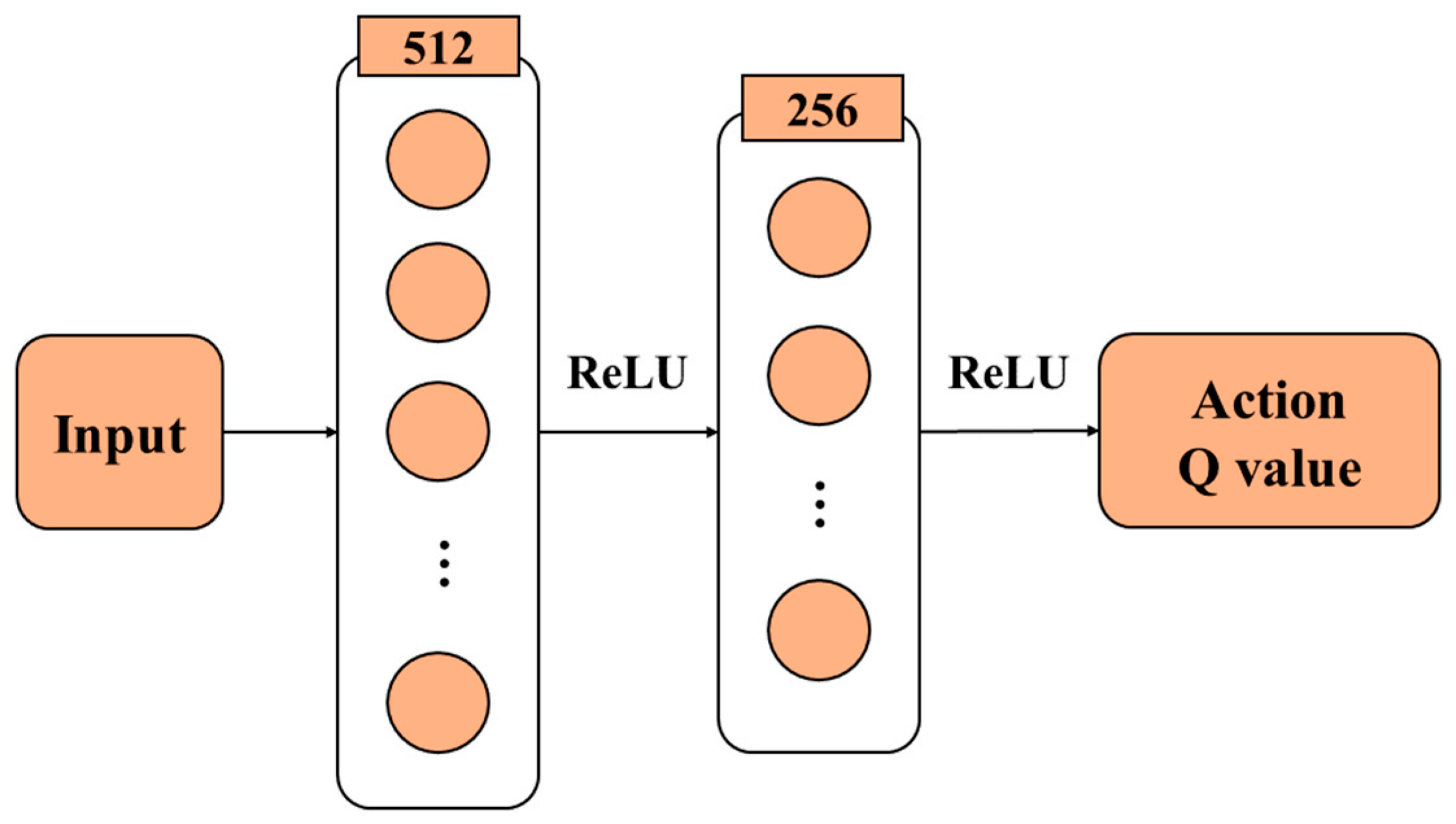
3.2.2. Estimation Network

In reinforcement learning methodologies, updates occur based on the reward of the current moment and the value estimation of the subsequent moment. Owing to the inherent volatility within the data, each iteration may introduce fluctuations that promptly influence the computation in the ensuing iteration, rendering the attainment of a stable model challenging. To reduce the impact of related problems, it is necessary to decouple the two parts of the current time and the next time value estimation as much as possible, thus introducing a dual network structure. The estimation network and the target network have the same structure, where the estimation network is used to interact with the environment, obtain interaction samples, and predict the Q estimate of the current action to select the best action.

3.2.3. Target Network

The target network is used to calculate the target Q value based on the state of the next step. After a specific number of iterations, the parameters of the estimated network are synchronized with the target network. As a result, the parameters of the target network become older than those of the estimated network. The approach of utilizing the subsequent state to compute the target value in the target network model maintains stability for a defined duration. This temporal stability diminishes the association between the current Q value and the target Q value to a certain extent, thereby enhancing the overall algorithmic stability.

3.2.4. Experience Pool

Reinforcement learning methods will directly use the data generated by the interaction to learn and not retain the generated samples. To ensure sufficient training samples and prevent more time to interact with the environment and collect samples after discarding samples, the experience pool replay mechanism is used, that is, to establish an experience pool for storing sample data of past experiences and help to disrupt the correlation between samples. The experience pool stores samples from interactions with the environment in chronological order. If the experience pool is already full, the new sample overwrites the oldest sample. When the network needs to update parameters, a sample is randomly selected from the experience pool for training. The training effect of this method is more stable, which not only improves the utilization rate of samples but also reduces the correlation of data.
The DQN training process is shown in Figure 2. The agent randomly selects behaviors from the environment to obtain experience tuples and stores them in the experience pool for continuous updates. Then, as the input of the estimation network and the target network, the output difference between the two is input as a loss function, the weight parameters of the estimated network are updated with the gradient descent algorithm, and actions are taken again. The estimated network copies the parameters to the target network after a fixed number of iterations. When the network training converges, the estimated network will approximate the optimal value function and realize the purpose of optimal strategy learning.

3.3. Hindsight Experience Replay Mechanism

In the DQN algorithm, an experience playback mechanism is adopted. This mechanism aims to create an experience pool for storing sample data generated throughout the training process. Samples are drawn from this pool using random selection to disturb interdependencies between samples. Sample forms are generally ( s t , a t , s t + 1 , r t ). For the robot obstacle avoidance environment, if there are only two reward forms of obstacle and goal point, then only a binary reward of r t = 0 , 1 will be generated. During the training phase, although the agent intends to move toward the direction of the highest cumulative reward, the cumulative reward value is always kept near zero. As a result, the neural network updates slowly, hindering model convergence. Therefore, it is hoped that the problem of reward sparsity can be solved by reducing useless experience ( r t = 0 ) and increasing valuable experience without modifying the environment.
Considering that obstacle avoidance is the task characteristic of training the agent to reach several different target points, the determination of the target value and the organization of the experience pool encompass not only the state “s” but also the goal “g”. Adding a goal only influences the agent’s decision-making regarding actions without impacting the dynamic alterations within the environment. This insight allows for the adaptation of goals within the trained experiences, accompanied by the corresponding reward value adjustments. This strategic maneuver facilitates the expansion of the current experience pool and significantly augments the reservoir of valuable experiences [48].
Fixed goal g in each training round and stored experience ( s t , a t , s t + 1 , r t , g ). At the end of this round of training, a hindsight experience replay is conducted for the experience generated in this round. From the states encountered in the whole training process, k states are randomly selected as the replay goal. Based on this goal, r t in this round of experience is judged again based on (1):
r t = 1       s t + 1 = g 0       s t + 1   g
After the new experience ( s t , a t , s t + 1 , r t , g ) is stored in the experience pool, the next round of learning begins.
Through effectively assimilating insights from sparse binary rewards, the hindsight experience replay mechanism maximizes the intrinsic value of the data, circumventing the necessity for intricate reward function engineering [25]. This mechanism can be perceived as a variant of a concealed curriculum. This is because the replayed objectives inherently progress from elementary, and sometimes arbitrary, agents to more intricate goals without necessitating any alterations in the distribution of initial environmental states.

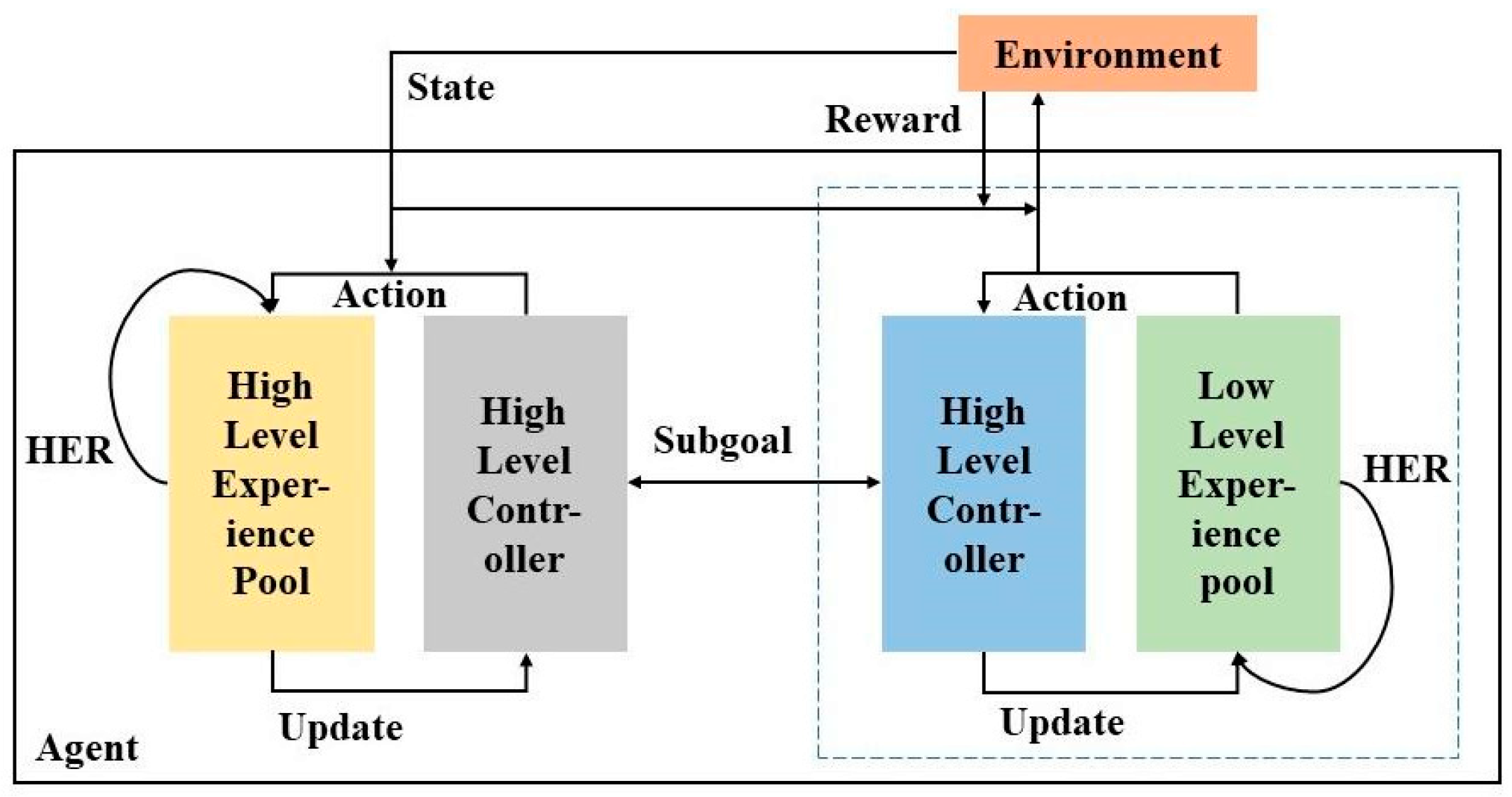
3.4. Algorithm Structure

The GDH-DQN algorithm is a hierarchical reinforcement learning method based on subgoals that consists of two layers of deep reinforcement learning algorithms; each layer adopts the DQN algorithm. The Deep Q-Network (DQN) algorithm represents a pivotal advancement in the domain of reinforcement learning. Characterized by its simplicity and ease of implementation, the DQN algorithm’s most notable feature is its capability for offline learning. This attribute enables DQN to effectively harness past experiences, thereby conferring a significant advantage in environments that are volatile or hazardous. In contrast to the Asynchronous Advantage Actor-Critic (A3C) algorithm, which necessitates continuous interaction with the environment for learning [49], DQN’s ability to learn from historical data stands as a distinctive and beneficial characteristic. Simultaneously, the simplistic network architecture of DQN, compared to other more complex and advanced algorithms, imposes lower computational resource requirements, making it more suitable for scenarios such as Mars exploration where computational resources are limited.
DQN has an experience replay mechanism, so it can be modified for samples in the experience pool, thus improving the efficiency of sample use. To solve the sparse reward problem and the non-stationary problem of parallel training, the hindsight experience replay mechanism is added to each layer to correct the sample, generate the forward sample guidance algorithm training direction, and improve the algorithm performance. The block diagram of the GQH-DQN algorithm is shown in Figure 3.
The low layer of the GDH-DQN algorithm is the obstacle avoidance control model, and the upper layer is the goal selection model. The design details of each layer model are as follows:

3.4.1. Low-Level Obstacle Avoidance Control Model

The low-level controller is mainly used for obstacle avoidance control, which selects appropriate actions for the mobile robot to avoid obstacles so as to achieve the effect of safe navigation from the starting point to the target point. However, due to the sparse reward problem in the navigation process, the agent cannot obtain effective samples in the training process, and the training efficiency decreases. Therefore, the hindsight experience replay mechanism is adopted to modify the goal passed by the high-level and change the original goal to the arrived state, thus changing the obtained reward value, generating positive samples, and solving the sparse reward problem.
Taking the sample {current state = s 0 , action = a, reward = 0, next state = s 1 , goal = g 0 } as an example, the agent takes g 0 as the target to explore, moves from state s 0 to s 1 after taking action a, and then the agent stops exploring due to step limitation and other reasons.
This means that the training round is over without reaching the goal. The samples generated in this round are not optimal strategies, so the hindsight experience replay mechanism can be used to select the next state reached in the samples as the goal of the current level, so as to ensure that there will be samples with positive rewards.
Therefore, the next state s 1 in the original sample is selected as the goal, and the sample is modified to {current state = s 0 , action = a, reward = 1, next state = s 1 , goal = g 1 }. After the sample is modified, the reward value is no longer 0, and such a sample can provide more information for the training of the agent, thus improving the training efficiency of the algorithm.
During the training process, if a goal has not been reached after a long time of exploration, then the goal is not suitable for the subgoal of the initial state at that time. In order to reduce the influence of this invalid target and shorten the invalid exploration time in the training process, the parameter of exploration step number is set in the low-level obstacle avoidance control model. Once the number of steps is exceeded, the training round is stopped.
The state space of the low-level controller is the set of all states that the agent can reach, and the action space is still four discrete actions.

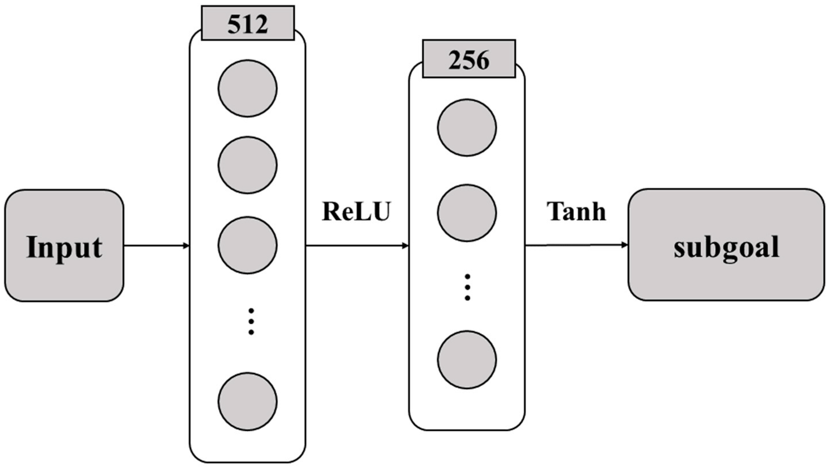
3.4.2. High-Level Target Selection Model

The high-level controller is mainly used to select subgoals from the set of possible states. Therefore, the original complex large-scale navigation process can be simplified to select feasible node target sequences at the high-level and perform navigation tasks step by step according to the provided subgoals at the low-level.
The reasons for non-stationary problems in hierarchical reinforcement learning are as follows: On the one hand, the constantly adjusted strategies at the low level will lead to unstable empirical data at the high-level [50]. On the other hand, the algorithm at the low level adopts random strategies for coupling exploration into the sampling process, and the random behavior leads to unstable state distribution, which affects the learning transfer function at the high level. For example, the ε-greedy strategy used in DQN has a certain probability of taking a random action. To allow the high-level and the low-level to train in parallel and obtain stable data, the high-level controller adopts the hindsight experience replay mechanism. After each training round, the action in the sample generated by the round is modified to the actual state reached by the low level, which is equivalent to generating the optimal strategy sample of the low level to solve the non-stationary problem.
Taking the sample {current state = s 0 , action = a 0 , reward = 0, next state = s 1 , goal = g } as an example, the final goal of the navigation task is g, the original action of the high level is g 0 , that is, the subgoal g 0 is selected for the low level. However, the actual state reached by the agent is s 1 . Therefore, to generate the optimal strategy sample, the original sample is modified to {current state = s 0 , action = a 1 reward = 1, next state = s 1 , goal = g }.
The pseudo-code is shown in Algorithm 1.
Algorithm 1 GDH-DQN algorithm
01: Initial high-level and low-level controller parameters
02: Initialize the experience pool capacity and learning rate of each layer
03: for episodes ← 1 to N do
04:   Initialization state s 0 , goal g
05:   Execute the train function in layers and complete hindsight experience replay
06:   Network parameters are synchronized after an update period
07: end for
08: function Train ()
09:   Initializes the layer state and goal
10:   for within exploration steps or have not yet reached the goal do
11:    The action is obtained using the ε-greedy strategy
12:    Take action and change the state to the next state
13:    The experience pool stores samples
14:   end for
15:   The low-level performs hindsight experience replay
16:   The high layer replays based on the low layer execution
17: end function
After sample modification, the sample obtained by the high-level is not only in line with the optimal strategy but also a valuable positive sample, which effectively solves the non-stationary problem and the sparse reward problem.
Because the number of exploration steps is set at the low level, when the number of steps is reached, the agent will stay in a certain state, and after the hindsight experience replay of the high-level, a certain state will be treated as a generated subgoal and stored as a sample in the experience pool. In this way, the high-level strategy can find the goal that can be reached within the specified number of steps, improve the selection probability of some reasonable states, and eliminate unreasonable subgoal states.
The action space and state space of the high-level model are the same, and both are the state space of the low-level obstacle avoidance control model, that is, the state position that each agent may reach. Places in the high state space should remove certain obstacles to prevent them from being selected as subgoals. However, this method is not easy to implement, not only because the environment is unknown and it is impossible to eliminate the obstacle coordinates in advance, but also because if the state space of the high-level and the low-level are different, it will occur that the low-level reaches an unreasonable state position during training, and after the hindsight experience replay of the high-level, subgoals that do not belong to the state space of the high-level will appear. That said, you cannot fix this problem by modifying the state space, so consider engaging in a hindsight experience replay process. When the low-level agent encounters an obstacle, it will obtain a reward value of −1. In order to avoid the value function of the high-level policy starting from such a state, the high-level will not play back the experience after the state, preventing the high-level from selecting this obstacle state several times after generating positive samples.

4. Experimental Verification

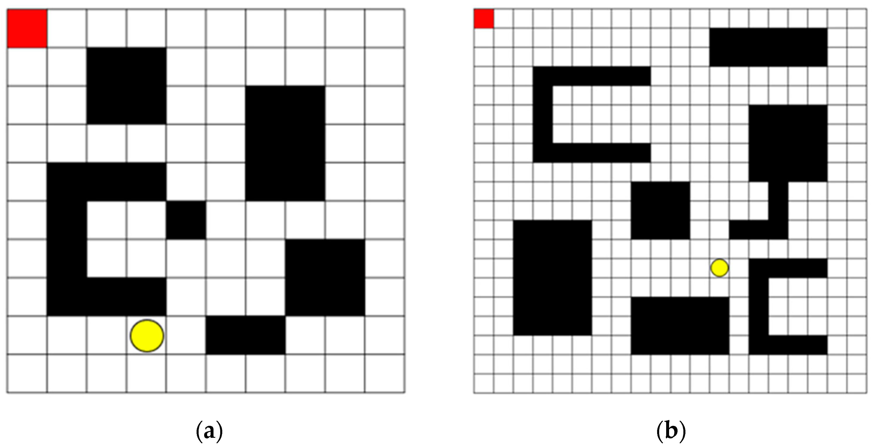
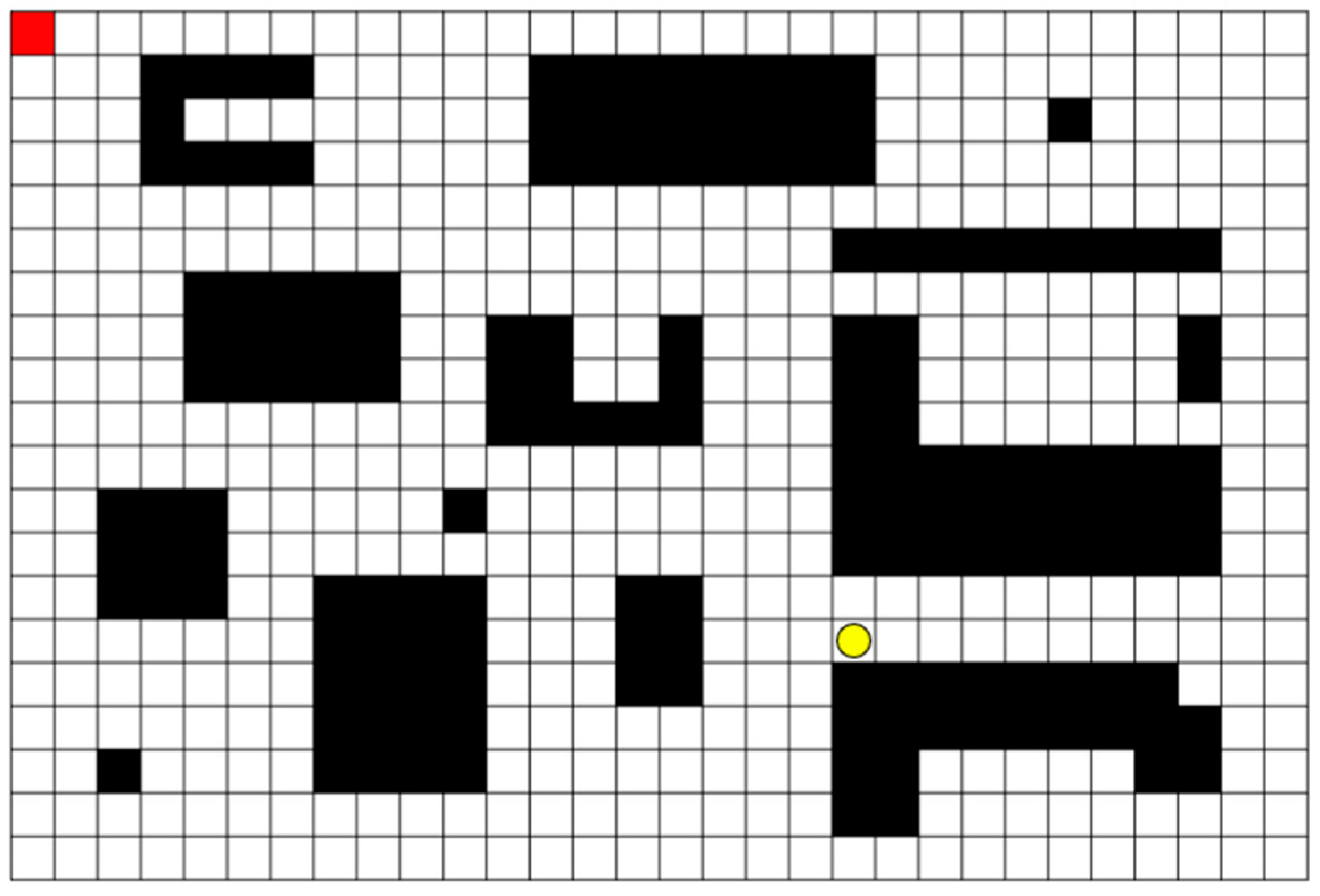
4.1. Experimental Environment

Due to its simplicity, effectiveness, and straightforward implementation, the grid environment has found extensive utility in the realm of path planning [51]. This technique partitions the two-dimensional map into discrete rectangular grid units, with the grids being assigned values corresponding to obstacles or open spaces. Modeling is accomplished via a two-dimensional matrix, with grids devoid of obstacles set to 0 and those with obstacles set to 1. The quantity of information contained within the grid environment is contingent upon the grid size. Opting for smaller grids yields higher environmental resolution and augmented information storage, but slower decision-making. Conversely, selecting larger grids results in reduced environmental resolution, diminished information storage, and faster decision-making. However, this comes at the cost of weakened pathfinding capabilities within densely obstacle-laden environments, consequently impacting the precision of the obtained paths [52].
Based on the Mars surface features depicted in Figure 4 [53], which exhibit a large environmental range and densely packed obstacles, we have established a rasterized map with the same characteristics. The black grid represents an immovable obstacle, resembling the large and dense nature of the Martian terrain. Furthermore, grid maps of varying sizes have been developed. Each grid is equivalent to the size of a Mars rover (3 m × 3 m). At this scale, the 20 × 20 and 20 × 30 grids can effectively replicate a wide range of the Martian environment. This simplified yet distinctive map has been utilized for experimental validation of the algorithm’s efficacy.
Gym is a toolkit for developing and comparing reinforcement learning algorithms under openAI (San Francisco, CA, USA) and provides the environment required for reinforcement learning. Gym makes no assumptions about the structure of the agent and is compatible with any digital computing library (such as TensorFlow (Mountain View, CA, USA) or Theano (Montreal, QC, Canada)) that can be used to formulate reinforcement learning algorithms. These environments have shared interfaces that make it possible to write regular algorithms. Therefore, this paper uses a Gym to build a grid environment for reinforcement learning training. The action space in reinforcement learning determines the output of the decision. According to the characteristics of the raster environment, this paper adopts a discrete action space, including the four actions of up, down, left, and right in the first-person perspective, to move vertically and horizontally in the raster, and refers to 0, 1, 2, and 3 numbers in the algorithm. We utilize a discrete action space, a choice that adheres to the regulations governing the agent’s behavior within the grid while simultaneously streamlining the action process. This simplification contributes to algorithmic convergence. In summary, we employ a discrete action space for simulating operations on the grid.

4.2. Neural Network and Parameter Design

Different from the neural network of a single-layer algorithm, the action output range of the high-level target selection model should be the size range of the map. Therefore, it is necessary to consider the normalization of the output of the neural network and then expand the output to the specified range according to the size of the map.
The design of the high-level neural network is illustrated in Figure 5, featuring 512 × 256 fully connected layers. The activation function for the hidden layers is ReLU, while the Tanh function is used for the output layer. Tanh not only restricts the output to the range [−1, 1] but also offers a fast convergence rate. Once the neural network output is obtained, it must be further processed to match the range of the map. The calculation method is described in (2).
a = a 0 * k + b
where a 0 is the output of the neural network, a is the subitem point obtained, k represents the map range, and b is the bias quantity. If the map parameters are L in length and W in width, then k is the vector [L/2, W/2] and b is the vector [L/2, W/2]. After calculation, the final coordinate range is [0, L] horizontally and [0, W] vertically. Since the calculated range is continuous, whereas each coordinate on the raster map is an integer, the computed coordinates should be rounded. This ensures the output of the high-level neural network aligns perfectly with the action space of the high-level model.
The architecture of the low-level neural network is depicted in Figure 6, mirroring the high-level neural network structure. The low-level action selection process involves computing the Q values for all potential actions and choosing the action with the highest Q value. As there is no requirement to restrict the output range of the neural network, the hidden layer activation function is set to ReLU, obviating the need for any specialized design considerations.
Reward shaping necessitates the pre-design of a reward function based on prior knowledge to furnish the agent with supplemental reward information to overcome the sparse reward problem. This paper conducts a comparative analysis of the reward-shaping methods employed in the experiment. Our aim is to guide the agent to maintain proximity to the target point while simultaneously minimizing the time required and the path cost incurred to reach the target. To achieve this, a reward function is devised wherein the robot garners progressively larger rewards as it draws closer to the designated target point. The reward function of the low-level obstacle avoidance control model is shown in (3).
R e w a r d = 1 ,   |   ( x r o b o t , y r o b o t ) = ( x o b s t a c l e , y o b s t a c l e )       1 ,   |   ( x r o b o t , y r o b o t ) = ( x g o a l , y g o a l )       0 ,   |   o t h e r w i s e
x r o b o t , y r o b o t indicates the current position of the mobile robot, x g o a l , y g o a l indicates the subgoal position provided by the high layer, and x o b s t a c l e , y o b s t a c l e indicates the obstacle position.
R e w a r d = 1 ,   |   ( x r o b o t , y r o b o t ) = ( x o b s t a c l e , y o b s t a c l e )       1 ,   |   ( x r o b o t , y r o b o t ) = ( x a c t i o n , y a c t i o n )       0 ,   |   o t h e r w i s e
where ( x a c t i o n , y a c t i o n ) indicates the subgoal position that the high-level outputs in the form of an action. When the reward value is −1, no hindsight experience replay is performed.
The algorithm hyperparameter settings in this chapter are shown in Table 1. It is important to note that when a parameter is not explicitly distinguished between the low layer and the high layer in the table, it is shared and has an equivalent size for both layers. Furthermore, the exploration steps specified for each round are proportional to the dimensions of the map, with the parameter value being the aggregate of the length and width of the grid map.

4.3. Analysis of Computational Complexity and Resource Consumption

The Deep Q-Network (DQN) model used in this study is relatively simple, comprising two hidden layers and one output layer with 256, 64, and 4 neurons, respectively. We use the total number of parameters and Floating Point Operations per Second (FLOPs) to evaluate the model’s computational complexity and resource requirements [54,55]. The model has a total of 17,988 parameters and involves 18.31 KMac FLOPs, indicating that the model is computationally lightweight and does not rely on a GPU for inference, making it suitable for operation in the highly resource-constrained environment of the Mars rover.
The computer used in this experiment is equipped with an Intel Core i7-11700K processor(Intel, Santa Clara, CA, USA), with a base clock frequency of 3.60 GHz and a maximum turbo frequency of up to 5.0 GHz. The CPU usage of the process running the model was measured at 0.0%, indicating that the model’s demand on CPU resources during execution is extremely low and can be practically ignored. This suggests that even with multiple inference operations, the model would not place a significant burden on the system’s central processing unit (CPU). Additionally, the model’s memory usage was measured at 239.484375 MB, which is relatively low compared to typical machine learning tasks [56], demonstrating good memory efficiency during execution.
Execution time measurements showed that the model’s inference speed is extremely fast, with single inference operations taking between 8.4 microseconds and 230.6 microseconds, with a median inference time of around 10 microseconds. This indicates that the model is highly efficient for single inference operations, and its low-latency characteristics make it suitable for navigation tasks in Mars exploration.
Considering the computational resources of the Mars rover, which is equipped with a RAD 750 PowerPC CPU(BAE Systems, Manassas, VA, USA) running at 133 MHz [32], and assuming the RAD 750 CPU is a scalar processor, the maximum number of operations per second (FLOP/s) would be 133 MFLOP/s. Based on the computational complexity and memory requirements of the DQN model in this study, along with factors such as instruction latency and resource contention, it is conservatively estimated that the time required to run inference tasks on the rover’s CPU would be in the range of tens of microseconds. Therefore, this model can provide real-time decision-making and navigation support on the Mars rover, making it well-suited for deployment in Mars exploration tasks where quick response and low computational resource usage are critical.

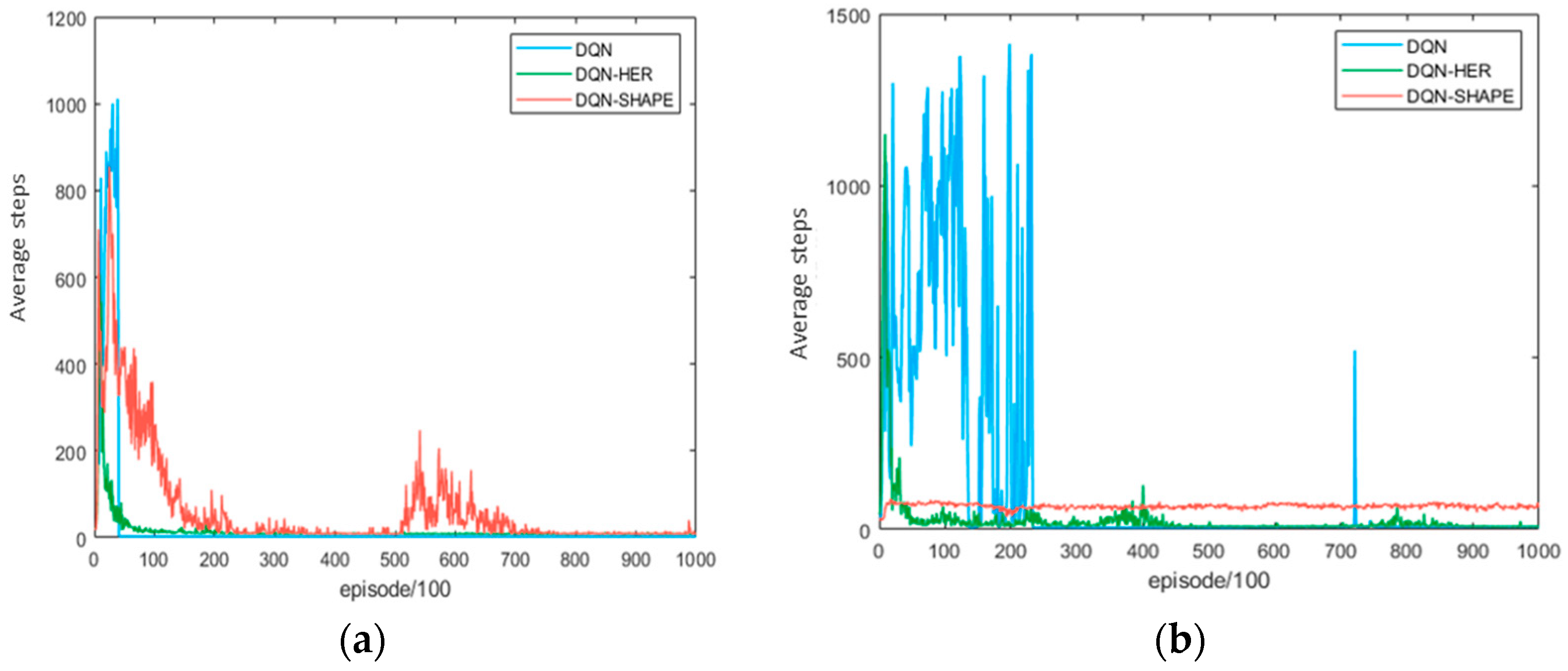
4.4. Single-Goal Experiment

In order to improve the sparse reward problem and improve the obstacle avoidance success rate between goals, we added the hindsight experience replay mechanism to the low-level obstacle avoidance control model so that the agent can learn from the failure experience and improve the sample utilization. When there is only one goal in the environment, GDH-DQN only needs to use the low-level obstacle avoidance control model to make decisions. To verify the effectiveness of the obstacle avoidance model of the algorithm, we designed a set of experiments to compare the DQN algorithm, the DQN-HER algorithm (low-level of GDH-DQN), and the DQN algorithm using the reward shaping method (DQN-SHAPE) in the presence of a single goal in the grid environment.
We designed maps of two sizes, 10 × 10 and 20 × 20, as shown in Figure 7. The red square indicates the starting position of the agent, and the yellow circle marks the target destination, which is randomly generated for each iteration. The static black grids represent immutable obstacles that remain fixed throughout the training process.
Following 100,000 epochs of training, the results are depicted in Figure 8. The figure illustrates the training progress, with the x-axis indicating the number of training epochs divided by 100 and the y-axis representing the navigation success rate, which is the number of successful training epochs out of every 100. The success rate graph is obtained from multiple experimental iterations, where the solid line denotes the average success rate across these iterations, and the shaded region illustrates the fluctuation range of the algorithm’s navigation success rate. The training curve demonstrates that the DQN-HER approach achieves convergence to the optimal path within the allocated training timeframe across various grid environments. Moreover, the convergence speed is swifter, and the success rate is higher compared to the other two methods. By observing the shadow of the training curve, it can be seen that the shadow area of the DQN-HER algorithm is smaller than that of the DQN-SHAPE and DQN algorithms, indicating that the success rate of the DQN-HER algorithm has less fluctuation and its performance is more stable.
The average number of steps is shown in Figure 9. In this figure, the x-axis corresponds to the number of training rounds divided by 100, while the y-axis represents the mean number of steps required for navigation during each set of 100 training rounds.
Integrating the analysis of the navigation success rate, the DQN-HER algorithm exhibits rapid convergence, capable of reaching the target point with a reduced number of steps while sustaining a high success rate. The DQN-SHAPE algorithm performs slightly less effectively than DQN-HER, requiring a greater average number of steps to converge. The DQN algorithm displays significant fluctuations in the average number of steps, suggesting that it often wanders aimlessly in the environment, engaging in indiscriminate exploration. At the end of the training, the DQN’s average number of steps converges to a lower level than the DQN-HER, which occurs because the DQN is prone to bumping into obstacles during navigation, resulting in the end of the training round and thus fewer steps.
The navigation success rate of each algorithm is shown in Table 2. The table includes the highest success rate observed across multiple experiments and the average success rate, which is calculated by dividing the total number of successful trials by the total number of training rounds. In the 10 × 10 maps, DQN-HER achieved the highest navigation success rate of 94%, outperforming DQN-Shape by 6% and DQN by 17%. On the 20 × 20 maps, DQN-HER reached a high of 81%, showing a 20% improvement over DQN-SHAPE and a 38% improvement over DQN. The average success rates for DQN and DQN-SHAPE are lower due to factors such as slower convergence speeds and performance instability, which affect the overall calculated averages.
The comparative analysis of the various metrics clearly demonstrates that the DQN-HER algorithm not only achieves a higher success rate but also exhibits greater resilience to variations in map size. As the map dimensions increase, the performance of the DQN and DQN-SHAPE algorithms significantly degrades. In contrast, the DQN-HER algorithm experiences minimal performance fluctuations and continues to preserve robust navigation capabilities, even on larger maps.
In conclusion, the DQN-HER algorithm, which serves as the low-level component of the GDH-DQN framework, outperforms the original DQN and the reward shaping method DQN-SHAPE in terms of navigation success rate, stability, and efficiency in reaching the target point with fewer steps. DQN-HER effectively addresses the sparse reward issue and equips mobile robots with robust mapless navigation capabilities and enhanced intelligent decision-making abilities.

4.5. Multi-Goals Experiment

4.5.1. Comparative Experimental Design

The GDH-DQN algorithm introduced in this chapter is a two-tiered architecture that integrates the DQN algorithm with the addition of the hindsight experience replay mechanism to each layer to enhance the algorithm’s performance. To validate the efficacy of the enhanced GDH-DQN algorithm, an ablation study is conducted, comparing it to the H-DQN algorithm, which lacks the hindsight experience replay mechanism. This experiment aims to assess the performance of the single-layer DQN-HER algorithm against the GDH-DQN algorithm, demonstrating the impact of the proposed hierarchical structure and the hindsight experience replay on navigation success.
To underscore the advantages of the GDH-DQN algorithm in navigating expansive environments, this chapter designs a series of maps and incorporates dead-end structures to enhance environmental complexity. In addition to the 10 × 10 and 20 × 20 maps in Figure 7, an additional 20 × 30 map is introduced, as depicted in Figure 10, further challenging the navigation algorithms with a larger and more intricate space.

4.5.2. Performance Index Design

The algorithm in this chapter adds a restriction on the number of exploration steps in the training process, so the performance index is different. In addition to the highest and average success rates in each environment, add collision and timeout rates. The collision rate is the proportion of the training round that is stopped due to hitting an obstacle and is calculated as the number of obstacles encountered per 100 training rounds. The timeout rate is the percentage of a training round that is stopped because it exceeds the required number of exploratory steps, calculated as the number of steps exceeded per 100 training rounds. The quantitative relationship between indicators is in (5):
Success rate + Collision rate + Timeout rate = 100%
The training outcomes are presented in Figure 11. A comparison of the success rate curves reveals that the GDH-DQN algorithm outperforms the other two algorithms, with a peak navigation success rate of 100%, suggesting that GDH-DQN is resilient to the complexities introduced by structures such as dead ends. The convergence speed of the DQN-HER algorithm is notably slower in this chapter due to the increased number of exploration steps, while GDH-DQN and H-DQN converge within the specified number of training rounds, indicating their effectiveness in learning optimal strategies and their rapid learning capabilities. The size of the shaded areas in the figure reflects the variability in algorithm performance: the broad shadow area for H-DQN signifies significant fluctuations and a non-stationary issue during training, whereas the narrow shadow area for GDH-DQN points to stable performance and effective mitigation of the non-stationary problem. Table 3 details the navigation success rates and other performance metrics for each algorithm. The collision rate and trek rate represent the navigation outcomes at the peak success rate, while the average success rate is the mean success rate across all training rounds.
In the 10 × 10 maps, GDH-DQN achieved a peak success rate of 100%, outperforming H-DQN by 1% and DQN-HER by 23%. In the 20 × 20 maps, GDH-DQN reached a high success rate of 93%, which was 12% higher than H-DQN and 29% higher than DQN-HER. In the 20 × 30 maps, GDH-DQN secured the highest success rate of 93%, surpassing H-DQN by 19% and DQN-HER by 42%. When comparing the collision rate and timeout rate, it is evident that the timeout rate exceeds the collision rate, suggesting that while the agent finds it relatively easier to learn obstacle avoidance, mastering the optimal path strategy presents a greater challenge. GDH-DQN demonstrates resilience to environmental variations, effectively learning both obstacle avoidance and optimal paths. Moreover, the average success rate of GDH-DQN is notably higher, indicating that the algorithm sustains a high success rate throughout training and consistently maintains a performance edge.
In summary, despite the constraints imposed by the number of exploration steps, the GDH-DQN algorithm maintains a high success rate even as environmental complexity increases. It effectively addresses the sparse reward problem and overcomes the non-stationary issue. In addition, GDH-DQN can learn the optimal strategy with fewer training steps, and the navigation path is shorter, indicating that it has a higher degree of intelligence and is suitable for large-scale and complex scene navigation.

4.6. Comprehensive Analysis of Performance Metrics

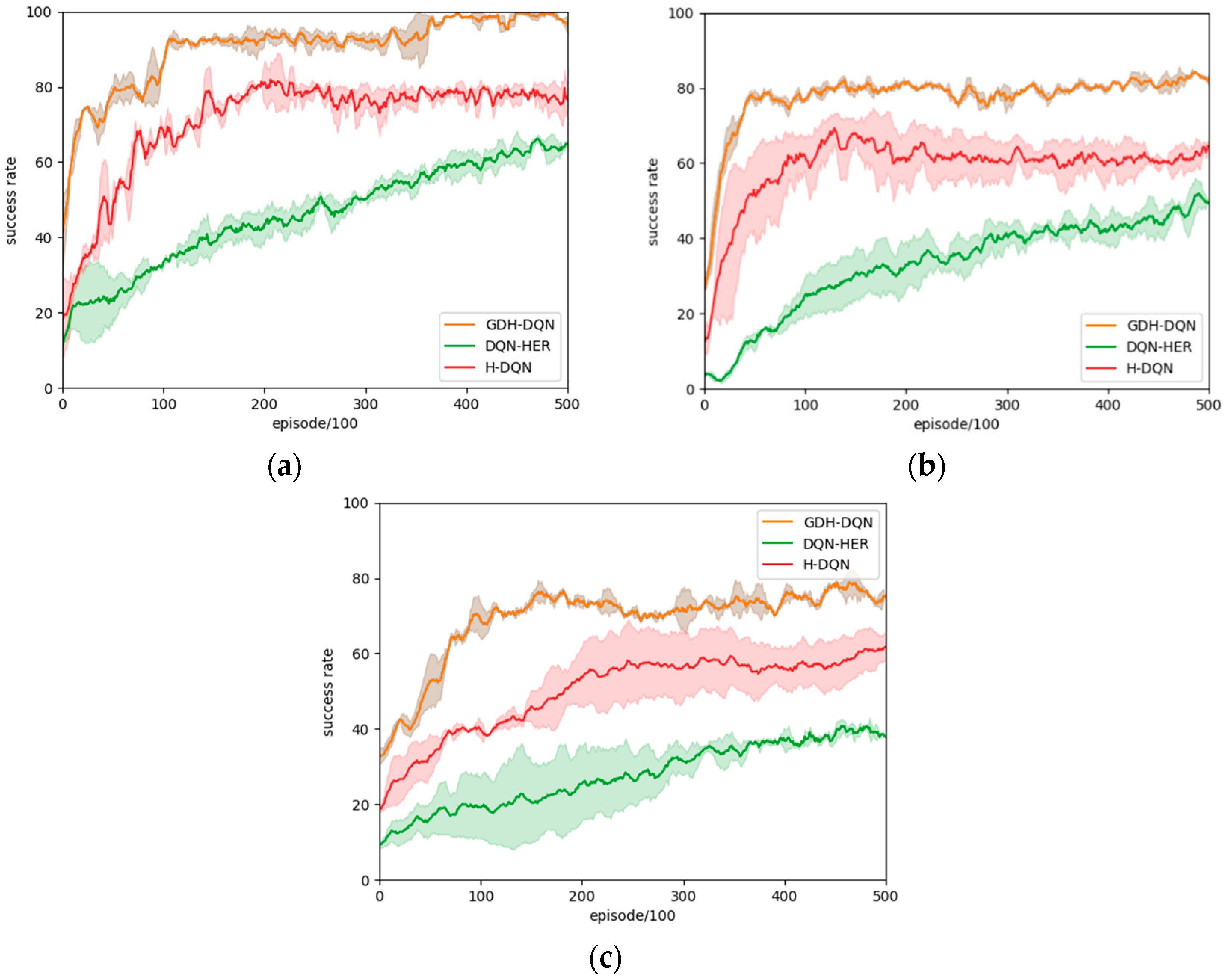
4.6.1. Navigation Success Rate

The results in Table 3 show that the GDH-DQN algorithm outperforms other baseline algorithms by more than 30% in terms of the highest navigation success rate. Notably, this advantage becomes more pronounced as the navigation scenario expands. In larger scenarios, the average navigation success rates of the baseline algorithms H-DQN and DQN-HER drop significantly to 50% and 28%, respectively, indicating that these two baseline algorithms are almost incapable of effective navigation. In contrast, GDH-DQN maintains an average success rate of 69% in these complex and large-scale scenarios. This demonstrates the superior navigation performance of GDH-DQN in the Mars surface navigation task under large-scale unknown scenarios.

4.6.2. Collision Rate

GDH-DQN and H-DQN both have a collision rate of 0% on a 10 × 10 map. However, on larger maps, GDH-DQN maintains a lower collision rate (2%) compared to H-DQN (10%) and DQN-HER (20%), indicating its superior obstacle avoidance capability. This suggests that even as the size of the environment increases, GDH-DQN almost never collides, demonstrating higher stability and safety.

4.6.3. Timeout Rate

The results in Table 3 show that GDH-DQN exhibits a lower timeout rate (5%) compared to H-DQN (16%) and DQN-HER (29%), especially on larger maps. This indicates that GDH-DQN can find shorter target paths more quickly. Analyzing this metric further reveals that while H-DQN and DQN-HER algorithms learn to avoid obstacles, they do not always find the optimal strategy and are prone to getting lost and timing out. This is especially true for DQN-HER, which has a high timeout rate (15%) even on the smallest maps. In contrast, the GDH-DQN algorithm demonstrates higher stability and intelligence.

4.6.4. Range of Success Rate Fluctuation

The shaded areas of the training curves in Figure 8 and Figure 11 indicate that GDH-DQN has smaller success rate fluctuations compared to H-DQN and DQN-HER, suggesting more stable navigation performance.

4.6.5. Convergence Speed

The training curve results in Figure 8, Figure 9, Figure 10 and Figure 11 show that GDH-DQN achieves higher success rates with fewer training steps compared to H-DQN and DQN-HER. This demonstrates the algorithm’s fast learning speed and quick convergence, as well as its ability to save computational resources.

4.6.6. Average Steps to Reach the Target

According to the data in Figure 9, the DQN-HER algorithm requires significantly fewer steps to reach the target compared to the DQN and DQN-SHAPE algorithms. This indicates that the DQN-HER algorithm not only has a higher navigation success rate but also finds shorter and more efficient paths, demonstrating higher efficiency in navigation.

5. Conclusions

This article primarily investigates a machine navigation algorithm for large-scale Mars exploration scenarios based on deep hierarchical reinforcement learning. A novel deep hierarchical reinforcement learning approach, GDH-DQN, is designed to decompose the inherently complex problem into multiple subtasks. This not only enhances sample efficiency but also mitigates the non-stationarity issues encountered during parallel training.
This algorithm is goal-driven, with a high-level target selection model choosing location nodes as short-term goals, while a low-level obstacle avoidance control model provides behavioral policies to achieve these short-term objectives, guiding the agent’s progress toward long-term navigation goals. Each level employs a Hindsight Experience Replay mechanism to enhance algorithm performance.
Various map sizes were used for experimentation, and the results validate the algorithm’s navigation advantages in Large-scale planetary exploration scenarios. Experimental data shows the algorithm’s high performance and strong adaptability when exploring complex navigation environments. In the future, with appropriate modifications, this algorithm can be extended to practical exploration applications in three-dimensional, unknown, and complex scenarios.

Author Contributions

Conceptualization, Z.Z., J.D., Y.C. and J.Y.; methodology, Y.C., J.Y. and B.Z.; software, Y.C. and J.Y.; validation, B.Z. and Q.W.; formal analysis, X.Z. and J.D.; investigation, X.Z. and Q.W.; resources, Z.Z., J.D., X.Z., Y.C., J.Y. and B.Z.; data curation, Y.C. and J.Y.; writing—original draft preparation, Y.C., J.Y. and B.Z.; writing—review and editing, Z.Z., Y.C., J.Y., B.Z., Q.W., X.Z. and J.D.; visualization, Y.C., J.Y. and B.Z.; supervision, Z.Z., J.D. and X.Z.; project administration, Z.Z.; funding acquisition, Z.Z. All authors have read and agreed to the published version of the manuscript.

Funding

This research received no external funding.

Data Availability Statement

The original contributions presented in the study are included in the article, further inquiries can be directed to the corresponding author.

Conflicts of Interest

The authors declare no conflicts of interest.

References

  1. Tao, Z.; Zhang, W.; Jia, Y.; Chen, B. Path Planning Technology of Mars Rover Based on Griding of Visibility-Graph Map Direction Search Method. In Proceedings of the CAC, Xiamen, China, 25–27 November 2022; pp. 6703–6707. [Google Scholar]
  2. Ropero, F.; Muñoz, P.; R-Moreno, M.D.; Barrero, D.F. A Virtual Reality Mission Planner for Mars Rovers. In Proceedings of the 2017 6th International Conference on Space Mission Challenges for Information Technology (SMC-IT), Madrid, Spain, 27–29 September 2017; pp. 142–146. [Google Scholar]
  3. Sun, S.; Wang, L.; Li, Z.P.; Gu, P.; Chen, F.F.; Feng, Y.T. Research on Parallel System for Motion States Monitoring of the Planetary Rover. In Proceedings of the 2020 5th International Conference on Communication, Image and Signal Processing (CCISP), Chengdu, China, 13–15 November 2020; pp. 86–90. [Google Scholar]
  4. Liu, J.; Li, H.; Sun, L.; Guo, Z.; Harvey, J.; Tang, Q.; Lu, H.; Jia, M. In-Situ Resources for Infrastructure Construction on Mars: A Review. Int. J. Transp. Sci. Technol. 2022, 11, 1–16. [Google Scholar] [CrossRef]
  5. Bell, J.F.; Maki, J.N.; Mehall, G.L.; Ravine, M.A.; Caplinger, M.A.; Bailey, Z.J.; Brylow, S.; Schaffner, J.A.; Kinch, K.M.; Madsen, M.B.; et al. The Mars 2020 Perseverance Rover Mast Camera Zoom (Mastcam-Z) Multispectral, Stereoscopic Imaging Investigation. Space Sci. Rev. 2021, 217, 24. [Google Scholar] [CrossRef] [PubMed]
  6. Ding, L.; Zhou, R.; Yu, T.; Gao, H.; Yang, H.; Li, J.; Yuan, Y.; Liu, C.; Wang, J.; Zhao, Y.-Y.S.; et al. Surface Characteristics of the Zhurong Mars Rover Traverse at Utopia Planitia. Nat. Geosci. 2022, 15, 171–176. [Google Scholar] [CrossRef]
  7. Zhou, R.; Feng, W.; Ding, L.; Yang, H.; Gao, H.; Liu, G.; Deng, Z. MarsSim: A High-Fidelity Physical and Visual Simulation for Mars Rovers. IEEE Trans. Aerosp. Electron. Syst. 2022, 59, 1879–1892. [Google Scholar] [CrossRef]
  8. Yang, G.; Liu, Y.; Guan, L. Design and Simulation Optimization of Obstacle Avoidance System for Planetary Exploration Mobile Robots. J. Phys. Conf. Ser. 2019, 1176, 032038. [Google Scholar] [CrossRef]
  9. Toupet, O.; Del Sesto, T.; Ono, M.; Myint, S.; vander Hook, J.; McHenry, M. A ROS-Based Simulator for Testing the Enhanced Autonomous Navigation of the Mars 2020 Rover. In Proceedings of the 2020 IEEE Aerospace Conference, Big Sky, MT, USA, 7–14 March 2020; pp. 1–11. [Google Scholar]
  10. Zhu, D.; Yan, M. Survey on Technology of Mobile Robot Path Planning. Control Decis. 2010, 25, 961–967. [Google Scholar]
  11. Hart, P.; Nilsson, N.; Raphael, B. A Formal Basis for the Heuristic Determination of Minimum Cost Paths. IEEE Trans. Syst. Sci. Cyber. 1968, 4, 100–107. [Google Scholar] [CrossRef]
  12. Khatib, O. Real-Time Obstacle Avoidance for Manipulators and Mobile Robots. In Proceedings of the 1985 IEEE International Conference on Robotics and Automation Proceedings, St. Louis, MO, USA, 25–28 March 1985; Volume 2, pp. 500–505. [Google Scholar]
  13. Hedrick, G.; Ohi, N.; Gu, Y. Terrain-Aware Path Planning and Map Update for Mars Sample Return Mission. IEEE Robot. Autom. Lett. 2020, 5, 5181–5188. [Google Scholar] [CrossRef]
  14. Daftry, S.; Abcouwer, N.; Sesto, T.D.; Venkatraman, S.; Song, J.; Igel, L.; Byon, A.; Rosolia, U.; Yue, Y.; Ono, M. MLNav: Learning to Safely Navigate on Martian Terrains. IEEE Robot. Autom. Lett. 2022, 7, 5461–5468. [Google Scholar] [CrossRef]
  15. Kaelbling, L.P.; Littman, M.L.; Moore, A.W. Reinforcement Learning: A Survey. J. Artif. Intell. Res. 1996, 4, 237–285. [Google Scholar] [CrossRef]
  16. Zhu, K.; Zhang, T. Deep Reinforcement Learning Based Mobile Robot Navigation: A Review. Tsinghua Sci. Technol. 2021, 26, 674–691. [Google Scholar] [CrossRef]
  17. Mnih, V.; Kavukcuoglu, K.; Silver, D.; Rusu, A.A.; Veness, J.; Bellemare, M.G.; Graves, A.; Riedmiller, M.; Fidjeland, A.K.; Ostrovski, G.; et al. Human-Level Control through Deep Reinforcement Learning. Nature 2015, 518, 529–533. [Google Scholar] [CrossRef] [PubMed]
  18. Mnih, V.; Kavukcuoglu, K.; Silver, D.; Graves, A.; Antonoglou, I.; Wierstra, D.; Riedmiller, M. Playing Atari with Deep Reinforcement Learning. arXiv 2013, arXiv:1312.5602. [Google Scholar]
  19. Schulman, J.; Wolski, F.; Dhariwal, P.; Radford, A.; Klimov, O. Proximal Policy Optimization Algorithms. arXiv 2017, arXiv:1707.06347. [Google Scholar]
  20. Mnih, V.; Badia, A.P.; Mirza, M.; Graves, A.; Lillicrap, T.; Harley, T.; Silver, D.; Kavukcuoglu, K. Asynchronous Methods for Deep Reinforcement Learning. In Proceedings of the 33rd International Conference on Machine Learning, PMLR, New York, NY, USA, 20–22 June 2016; pp. 1928–1937. [Google Scholar]
  21. Devidze, R.; Kamalaruban, P.; Singla, A. Exploration-Guided Reward Shaping for Reinforcement Learning under Sparse Rewards. Adv. Neural Inf. Process. Syst. 2022, 35, 5829–5842. [Google Scholar]
  22. Cimurs, R.; Suh, I.H.; Lee, J.H. Goal-Driven Autonomous Exploration Through Deep Reinforcement Learning. IEEE Robot. Autom. Lett. 2022, 7, 730–737. [Google Scholar] [CrossRef]
  23. Riedmiller, M.; Hafner, R.; Lampe, T.; Neunert, M.; Degrave, J.; Wiele, T.; Mnih, V.; Heess, N.; Springenberg, J.T. Learning by Playing Solving Sparse Reward Tasks from Scratch. In Proceedings of the 35th International Conference on Machine Learning, PMLR, Stockholm, Sweden, 10–15 July 2018; pp. 4344–4353. [Google Scholar]
  24. Shaping as a Method for Accelerating Reinforcement Learning|IEEE Conference Publication|IEEE Xplore. Available online: https://ieeexplore.ieee.org/document/225046 (accessed on 15 July 2024).
  25. Andrychowicz, M.; Wolski, F.; Ray, A.; Schneider, J.; Fong, R.; Welinder, P.; McGrew, B.; Tobin, J.; Pieter Abbeel, O.; Zaremba, W. Hindsight Experience Replay. In Proceedings of the Advances in Neural Information Processing Systems; Guyon, I., Luxburg, U.V., Bengio, S., Wallach, H., Fergus, R., Vishwanathan, S., Garnett, R., Eds.; Curran Associates, Inc.: New York, NY, USA, 2017; Volume 30. [Google Scholar]
  26. Jagodnik, K.M.; Thomas, P.S.; Van Den Bogert, A.J.; Branicky, M.S.; Kirsch, R.F. Training an Actor-Critic Reinforcement Learning Controller for Arm Movement Using Human-Generated Rewards. IEEE Trans. Neural Syst. Rehabil. Eng. 2017, 25, 1892–1905. [Google Scholar] [CrossRef]
  27. Brito, B.; Everett, M.; How, J.P.; Alonso-Mora, J. Where to Go Next: Learning a Subgoal Recommendation Policy for Navigation in Dynamic Environments. IEEE Robot. Autom. Lett. 2021, 6, 4616–4623. [Google Scholar] [CrossRef]
  28. Liu, W.W.; Wei, J.; Liu, S.Q.; Ruan, Y.D.; Zhang, K.X.; Yang, J.; Liu, Y. Expert Demonstrations Guide Reward Decomposition for Multi-Agent Cooperation. Neural Comput. Appl. 2023, 35, 19847–19863. [Google Scholar] [CrossRef]
  29. Dai, X.-Y.; Meng, Q.-H.; Jin, S.; Liu, Y.-B. Camera View Planning Based on Generative Adversarial Imitation Learning in Indoor Active Exploration. Appl. Soft Comput. 2022, 129, 109621. [Google Scholar] [CrossRef]
  30. Luo, Y.; Wang, Y.; Dong, K.; Zhang, Q.; Cheng, E.; Sun, Z.; Song, B. Relay Hindsight Experience Replay: Self-Guided Continual Reinforcement Learning for Sequential Object Manipulation Tasks with Sparse Rewards. Neurocomputing 2023, 557, 126620. [Google Scholar] [CrossRef]
  31. Feng, W.; Ding, L.; Zhou, R.; Xu, C.; Yang, H.; Gao, H.; Liu, G.; Deng, Z. Learning-Based End-to-End Navigation for Planetary Rovers Considering Non-Geometric Hazards. IEEE Robot. Autom. Lett. 2023, 8, 4084–4091. [Google Scholar] [CrossRef]
  32. Verma, V.; Maimone, M.W.; Gaines, D.M.; Francis, R.; Estlin, T.A.; Kuhn, S.R.; Rabideau, G.R.; Chien, S.A.; McHenry, M.M.; Graser, E.J.; et al. Autonomous Robotics Is Driving Perseverance Rover’s Progress on Mars. Sci. Robot. 2023, 8, eadi3099. [Google Scholar] [CrossRef]
  33. Wong, C.; Yang, E.; Yan, X.-T.; Gu, D. Adaptive and Intelligent Navigation of Autonomous Planetary Rovers—A Survey. In Proceedings of the 2017 NASA/ESA Conference on Adaptive Hardware and Systems (AHS), Pasadena, CA, USA, 24–27 July 2017; IEEE: Piscataway, NJ, USA, 2017; pp. 237–244. [Google Scholar]
  34. Why—And How—NASA Gives a Name to Every Spot It Studies on Mars—NASA. Available online: https://www.nasa.gov/solar-system/why-and-how-nasa-gives-a-name-to-every-spot-it-studies-on-mars/ (accessed on 15 July 2024).
  35. Paton, M.; Strub, M.P.; Brown, T.; Greene, R.J.; Lizewski, J.; Patel, V.; Gammell, J.D.; Nesnas, I.A.D. Navigation on the Line: Traversability Analysis and Path Planning for Extreme-Terrain Rappelling Rovers. In Proceedings of the 2020 IEEE/RSJ International Conference on Intelligent Robots and Systems (IROS), Las Vegas, NV, USA, 24 October 2020–24 January 2021; pp. 7034–7041. [Google Scholar]
  36. Kiran, B.R.; Sobh, I.; Talpaert, V.; Mannion, P.; Sallab, A.A.A.; Yogamani, S.; Perez, P. Deep Reinforcement Learning for Autonomous Driving: A Survey. IEEE Trans. Intell. Transport. Syst. 2022, 23, 4909–4926. [Google Scholar] [CrossRef]
  37. Faust, A.; Oslund, K.; Ramirez, O.; Francis, A.; Tapia, L.; Fiser, M.; Davidson, J. PRM-RL: Long-Range Robotic Navigation Tasks by Combining Reinforcement Learning and Sampling-Based Planning. In Proceedings of the 2018 IEEE International Conference on Robotics and Automation (ICRA), Brisbane, Australia, 21–25 May 2018; pp. 5113–5120. [Google Scholar]
  38. Al-Emran, M. Hierarchical Reinforcement Learning: A Survey. Int. J. Comput. Digit. Syst. 2015, 4, 137–143. [Google Scholar] [CrossRef] [PubMed]
  39. (PDF) Learning Representations in Model-Free Hierarchical Reinforcement Learning. Available online: https://www.researchgate.net/publication/335177036_Learning_Representations_in_Model-Free_Hierarchical_Reinforcement_Learning (accessed on 17 April 2024).
  40. Lu, Y.; Xu, X.; Zhang, X.; Qian, L.; Zhou, X. Hierarchical Reinforcement Learning for Autonomous Decision Making and Motion Planning of Intelligent Vehicles. IEEE Access 2020, 8, 209776–209789. [Google Scholar] [CrossRef]
  41. Trajectory Planning for Autonomous Vehicles Using Hierarchical Reinforcement Learning|IEEE Conference Publication|IEEE Xplore. Available online: https://ieeexplore.ieee.org/abstract/document/9564634 (accessed on 15 July 2024).
  42. Planning-Augmented Hierarchical Reinforcement Learning|IEEE Journals & Magazine|IEEE Xplore. Available online: https://ieeexplore.ieee.org/abstract/document/9395248 (accessed on 15 July 2024).
  43. Hierarchies of Planning and Reinforcement Learning for Robot Navigation|IEEE Conference Publication|IEEE Xplore. Available online: https://ieeexplore.ieee.org/abstract/document/9561151 (accessed on 15 July 2024).
  44. Between MDPs and Semi-MDPs: A Framework for Temporal Abstraction in Reinforcement Learning. Artif. Intell. 1999, 112, 181–211. [CrossRef]
  45. Han, R.; Li, H.; Knoblock, E.J.; Gasper, M.R.; Apaza, R.D. Joint Velocity and Spectrum Optimization in Urban Air Transportation System via Multi-Agent Deep Reinforcement Learning. IEEE Trans. Veh. Technol. 2023, 72, 9770–9782. [Google Scholar] [CrossRef]
  46. Han, R.; Li, H.; Apaza, R.; Knoblock, E.; Gasper, M. Deep Reinforcement Learning Assisted Spectrum Management in Cellular Based Urban Air Mobility. IEEE Wirel. Commun. 2022, 29, 14–21. [Google Scholar] [CrossRef]
  47. Yan, C.; Xiang, X.; Wang, C. Towards Real-Time Path Planning through Deep Reinforcement Learning for a UAV in Dynamic Environments. J. Intell. Rob. Syst. 2020, 98, 297–309. [Google Scholar] [CrossRef]
  48. Chen, J.P.; Zheng, M.H. A Survey of Robot Manipulation Behavior Research Based on Deep Reinforcement Learning. Robot 2022, 44, 236–256. [Google Scholar] [CrossRef]
  49. Biswas, A.; Anselma, P.G.; Emadi, A. Real-Time Optimal Energy Management of Multimode Hybrid Electric Powertrain with Online Trainable Asynchronous Advantage Actor–Critic Algorithm. IEEE Trans. Transp. Electrif. 2022, 8, 2676–2694. [Google Scholar] [CrossRef]
  50. Levy, A.; Konidaris, G.; Platt, R.; Saenko, K. Learning Multi-Level Hierarchies with Hindsight. arXiv 2018, arXiv:1712.00948. [Google Scholar]
  51. Ren, Y.Y.; Song, X.R.; Gao, S. Research on Path Planning of Mobile Robot Based on Improved A* in Special Environment. In Proceedings of the 2019 3rd International Symposium on Autonomous Systems (ISAS), Shanghai, China, 29–31 May 2019; IEEE: Piscataway, NJ, USA, 2019; pp. 12–16. [Google Scholar]
  52. Yue, P.; Xin, J.; Zhang, Y.; Lu, Y.; Shan, M. Semantic-Driven Autonomous Visual Navigation for Unmanned Aerial Vehicles. IEEE Trans. Ind. Electron. 2024, 71, 14853–14863. [Google Scholar] [CrossRef]
  53. Images from the Mars Perseverance Rover—NASA Mars. Available online: https://mars.nasa.gov/mars2020/multimedia/raw-images/ (accessed on 15 July 2024).
  54. Han, S.; Pool, J.; Tran, J.; Dally, W. Learning Both Weights and Connections for Efficient Neural Network. In Proceedings of the Advances in Neural Information Processing Systems; Curran Associates, Inc.: New York, NY, USA, 2015; Volume 28. [Google Scholar]
  55. He, K.; Sun, J. Convolutional Neural Networks at Constrained Time Cost. In Proceedings of the IEEE Conference on Computer Vision and Pattern Recognition (CVPR), Boston, MA, USA, 7–12 June 2015; pp. 5353–5360. [Google Scholar]
  56. Canziani, A.; Paszke, A.; Culurciello, E. An Analysis of Deep Neural Network Models for Practical Applications. arXiv 2016, arXiv:1605.07678. [Google Scholar]
Figure 1. Mars surface terrain from a large-scale perspective.
Aerospace 11 00692 g001
Figure 2. DQN training process.
Aerospace 11 00692 g002
Figure 3. Block diagram of the GDH-DQN algorithm.
Aerospace 11 00692 g003
Figure 4. Mars surface terrain, small-scale perspective.
Aerospace 11 00692 g004
Figure 5. High-level neural network structure.
Aerospace 11 00692 g005
Figure 6. Low-level neural network structure.
Aerospace 11 00692 g006
Figure 7. Grid map. (a) 10 × 10 grid map. (b) 20 × 20 grid. The red square marks the agent’s starting position, the yellow circle denotes the randomly generated target for each iteration, and the black grids are fixed obstacles throughout training.
Aerospace 11 00692 g007
Figure 8. Comparison of the navigation success rate of each algorithm. (a) 10 × 10 grid map. (b) 20 × 20 grid map.
Aerospace 11 00692 g008
Figure 9. Comparison of the average navigation steps of each algorithm. (a) 10 × 10 grid map. (b) 20 × 20 grid map.
Aerospace 11 00692 g009
Figure 10. 20 × 30 grid map. The red square marks the agent’s starting position, the yellow circle denotes the randomly generated target for each iteration, and the black grids are fixed obstacles throughout training.
Aerospace 11 00692 g010
Figure 11. Comparison of navigation success rates of different algorithms. (a) 10 × 10 grid map. (b) 20 × 20 grid map. (c) 20 × 30 grid map.
Aerospace 11 00692 g011
Table 1. Parameters of the GDH-DQN algorithm.
ParameterParameter Value
Experience pool capacity100,000
Batch size128
Learning rate0.001
Loss factor0.98
Exploration factor1 to 0
Sample proportion of HER4:1
Exploration steps per roundL + W
Table 2. Comparison of the navigation success rate of each algorithm.
AlgorithmDQN-HERDQNDQN-SHAPE
10 × 10
Highest success rate
94%77%88%
10 × 10
Average success rate
75.5%20.8%67.3%
20 × 20
Highest success rate
81%43%61%
20 × 20
Average success rate
63.6%12.6%36.7%
Table 3. Results of navigation training.
Test
Environment
AlgorithmHighest Success RateCollision RateTimeout RateAverage Success Rate
10 × 10GDH-DQN100%0%0%90.3%
H-DQN99%0%1%71.0%
DQN-HER77%8%15%45.9%
20 × 20GDH-DQN93%3%4%77.6%
H-DQN81%7%12%59.1%
DQN-HER64%13%23%33.1%
20 × 30GDH-DQN93%2%5%68.9%
H-DQN74%10%16%49.9%
DQN-HER51%20%29%27.7%
Disclaimer/Publisher’s Note: The statements, opinions and data contained in all publications are solely those of the individual author(s) and contributor(s) and not of MDPI and/or the editor(s). MDPI and/or the editor(s) disclaim responsibility for any injury to people or property resulting from any ideas, methods, instructions or products referred to in the content.

