A Physical and Spectroscopic Survey of the Lunar South Pole with the Galileo Telescope of the Asiago Astrophysical Observatory

Abstract

In recent years, interest in the Moon has grown exponentially, thanks mainly to space programs with strong international cooperation, such as the NASA Artemis program. Several scientific committees have identified the lunar south pole as the region of greatest interest for building a lasting and sustainable human settlement. However, the knowledge we have of this area is still limited. This work aims to provide a general overview of the main physical and morphological features of the lunar south pole and to propose a first iteration of spectroscopic observations within the visible range from the Asiago Astrophysical Observatory, giving a new and different perspective. The objective is to verify the feasibility of an Earth-based spectroscopic survey to detect water and the abundances of other volatiles and elements.

1. Introduction

In the last few years, we have been witnessing a new “Space Race” with numerous players united by the willingness to establish a sustainable human presence around the Moon environment. It is estimated that international space agencies assisted by a constantly growing number of private space companies have scheduled more than 140 missions towards the Moon during the decade 2023–2033 [1]; the greatest boost comes from the National Aeronautics and Space Administration (NASA) Artemis program closely followed by the analog Chinese and European lunar programs.

In such an animated framework, it is necessary to set up a series of guidelines to ensure the sustainability and long-term preservation of the lunar space and surface; for these reasons, the International Space Exploration Coordination Group (ISECG) has been created. It is a non-binding coordination forum of space agencies, which exchange information regarding interests, plans and activities in space exploration and which work together to strengthen both individual exploration programs and the collective effort. One of the most useful contributions is the setting up of a Global Exploration Roadmap (GER) that presents a shared international vision of human and robotic space exploration and reflects the exploration strategy and goals of the ISECG space agencies [2].

Due to the certified presence of water ice and its favorable environmental conditions, the lunar south pole has been pointed out as the most suitable region to accomplish proposed exploration goals and discovering its main features will be pivotal.

Within this context is placed this work whose aim is to provide an overview of the lunar south pole by highlighting the aspects that have made it an ideal candidate for future human settlement. In particular, the state-of-the-art analysis of this region is strengthened by a different perspective of the lunar south pole thanks to an experimental Earth-based spectroscopic survey within the visible range carried out from the Asiago Astrophysical Observatory (Asiago, Italy). The purposes of this survey are several, from the search of correlations with water abundance to the characterization of the lunar south pole areas to provide data and information for the design of future orbiter missions.

2. The Lunar South Pole

2.1. Physical Analysis

Our knowledge about the origin of the Moon is still limited and this underlines the importance of leading new scientific missions towards our natural satellites. Numerous theories on the Moon’s formation have been suggested but the most accredited one is that the Earth–Moon system formed out of the debris from a giant impact of a Mars-sized body (called Theia) and the proto-Earth. Then, the history of the Moon has been divided into five different geological periods defined through the radiometric dating of lunar surface samples: the pre-Nectarian (from 4.55 to 3.920 Gy ago), the Nectarian (from 3.92 to 3.85 Gy ago), the Imbrium (from 3.85 to 3.2 Gy ago), the Eratosthenian (from 3.2 to 1.1 Gy ago) and the Copernican (from 1.1 Gy to today). The main events that have affected the lunar surface are impact cratering and volcanism and so each group shows its own compositional and morphological features. Multi-band imaging and over 400,000 UV–VIS lunar spectra obtained by Clementine together with information from Earth-based observation gave a first global map of the mineral distribution over the lunar surface. Briefly, lunar surface materials are generally composed of two major types of materials: the lunar highland materials with their light color and the darker lunar mare materials [3]. The highlands are mostly composed of anorthosite (95% Ca-rich plagioclase and minor amounts of low-Ca pyroxene, olivine and clinopyroxene), Mg-rich rocks and KREEP rocks (rich in potassium (K), phosphorus (P) and rare-earth elements (REEs)); on the other hand, the 22 mares mainly spread on the near side are composed principally of basaltic lava flows, which in turn can be divided into three broad categories: high-Ti basalts, low-Ti basalts and high-Al, low-Ti basalts [4].

The resource potential of the Moon is not confined to the sphere of mining activities related to its formation but there is a wide range of potential lunar resources that might affect three different possible uses for lunar materials: the use of lunar materials to facilitate continued exploration of the Moon through In Situ Resource Utilization (ISRU), the use of lunar resources to simplify scientific and economic activity in the cislunar space and the importation of lunar resources to the Earth’s surface [5]. A long-term and sustainable human presence on the Moon has to include different types of resources like materials for Moon settlements construction, power systems, rocket fuel, etc.; eight major categories of lunar resources are summarized below [6] as follows:

• Water ice in polar areas;
• Non-polar hydrogen and oxygen implanted in the lunar regolith from the solar wind;
• Regolith-implanted helium-3 from the solar wind. Helium-3 could provide nuclear energy in a fusion reactor with the advantages that it is not radioactive and it would not produce dangerous waste products; all these hypotheses are under investigation;
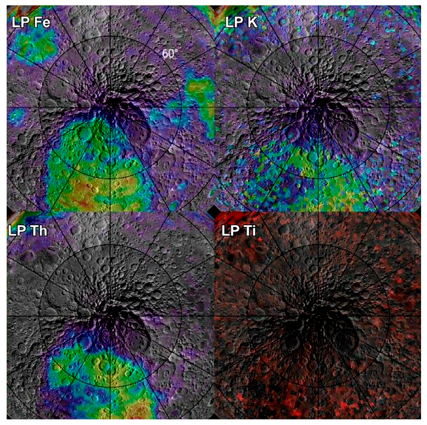
• Uranium and thorium in silica-rich domes and KREEP basalts on the lunar nearside, other important elements for the developments of space-based nuclear power and nuclear propulsion concepts;
• Basalt-hosted metals such as titanium, iron and aluminum (Papike et al. For example, the main Ti-bearing phase in lunar rocks is the mineral ilmenite particularly accredited for the retention of some solar wind-implanted volatiles and for ISRU oxygen extraction;
• Volatiles and elements of pyroclastic origin that include iron, zinc, cadmium, mercury, lead, copper and fluorine;
• Rare metals and platinum-group elements such as nickel, platinum, palladium, iridium and gold that may occur within segregated impact melt sheets and layered mafic extrusives;
• Other volatiles such as nitrogen, carbon and lithium in breccia or exhalative deposits.

This list as well our knowledge of the Moon’s geology is limited and based on remote sensing data from lunar probes and samples belonging only to a dozen landing sites principally at low latitude and on the near side.

Following this general introduction, we start exploring in detail our region of interest, the lunar south pole, investigating its main characteristics. The lunar south pole is situated inside the South Pole Aitken (SPA) basin, which is the largest and oldest discovered impact structure of the Solar System [7] with its 2600 km diameter and belonging to the pre-Nectarian period (ref. [8] offers a unified geological map of the lunar south pole region with a brief description of all the different geological areas); this massive impacts’ history has largely shaped the surface, making it extremely jagged. The Lunar Orbiter Laser Altimeter (LOLA) instruments on board the Lunar Reconnaissance Orbiter (LRO) highlight how the elevation ranges from about −7000 to +7000 m with slopes that can reach 80° (Figure 1a); this uneven topography extremely affects local illumination. Sunlight reaches the polar surface for less than 50% of the time even if a limited area near the rims of the Shackleton, De Gerlache and Nobile craters and the crest of the Malapert Massif can reach 80% illumination on average (Figure 1b); these results come from a simulation carried out by [9] over several years.

Certain areas located in unfavorable regions and with particularly deep depressions reside in constant darkness; these zones are called permanently shadowed regions (PSRs). Temperatures lower than 110 K are generally reached in these PSRs (Figure 2). Some of them have no direct line of sight to any non-permanently shadowed zones and so they can be shielded from the direct solar illumination but also from scattered light and thermal emission; in this case, they take the name of double permanently shadowed regions (DPSRs). Clearly, the reachable temperatures are lower, about 25 K. South pole PSRs are located beyond 80° latitude and occupy about 7.25% of the total surface area in this region while the total doubly shadowed area poleward of 85° latitude constitutes only 0.07% of the PSRs’ area in the region. These areas are of particular significance and make lunar poles different from any other region; due to their temperature, PSRs can harbor water ice while DPSRs could also potentially accommodate CO₂, CO, N₂, Ar and organic compounds delivered by the impacts of comets and meteorites [11]. Improving knowledge of these dark areas is essential to plan future missions to the PSRs like the NASA VIPER mission; the first results from the ShadowCam on board the KPLO seem to be encouraging, as transversal simulations of secondary illumination and topography imaging have revealed features of the surface of Shackleton and other PSR craters for the first time [12]. As well as the sunlight visibility, even the Earth visibility is strongly influenced by the surface morphology.

An integrated remote sensing analysis of the lunar south pole between different missions is necessary to create the best overview of the lunar south pole mineralogy and to enrich the interpretation of the spectroscopic data. The Moon Mineralogy Mapper data reveal the south polar region to be enriched in mafic minerals with respect to the highland crust, which represents an anomaly compared to the predominantly noritic character of the South Pole Aitken basin; this mafic anomaly is backed up by elemental abundance (for example, Fe, Th or K) data from the Lunar Prospector [13], suggesting the presence of a lower crust/upper mantle ejecta (Figure 3). Nonetheless, the remote sensing measurements were found to be slightly different from reality; the Chinese mission Chang’e 3 (2013) acquired the first in situ reflectance spectra of the lunar surface through a Visible Near-Infrared Spectrometer (VNIS), which demonstrated that the spectra of the uppermost soil detected by remote sensing exhibit substantial differences from that immediately beneath [14]. In situ spectra and samples from the interested regions will constitute vital elements for data analysis improvements and for the calibration of remote optical instruments.

2.2. Lunar Volatiles

The lunar south pole was certainly not indicated as the best human and robotic lunar base for its extreme environment but for its peculiarity of harboring ice and other volatiles; water ice may indeed be allowed to accumulate in permanently shadowed regions on airless bodies with a small tilt of the rotation axes in the inner solar system, as also happens for Mercury and Ceres [15]. The lunar surface is covered by a fragmental layer of rubbles (regolith) exposed to hydrogen as a proton; from the space environment, the solar wind implants protons into the lunar surface, which could be retained as molecular hydrogen, hydroxyl or molecular water. Another important contribution in the presence of water comes from water-bearing meteorites, asteroids and comets. But why is the presence of water and other volatiles so substantial? Water is a fundamental resource because it can be processed to make propellant, radiation-shielding and life-supporting consumables. One of the most efficient mixtures in a liquid propulsion system is based on hydrogen as fuel and oxygen as an oxidizer; currently, the average cost per kilogram to launch materials from the Earth’s surface to the LEO is roughly $35,000, which increases dramatically for escaping the Earth’s gravity. Hence, it becomes clear how cost-effective it would be to manufacture rocket propellant on the lunar surface. The physical form of water is not unique at grain-size scales (also known as the particle size, which is the average size of a sediment); there are several forms such as ice, frost, hydrated minerals, adsorbed molecules and soil mixtures that can constitute a key variable in the distribution [16]. Also, for this reason, the detection of lunar polar volatiles and their ensuing compositional analyses are not trivial; to achieve an exhaustive insight, it is necessary to cross-reference data from different detection techniques (imaging, spectroscopy, etc.) so as to compensate for the limitations of each.

The primary indicator of lunar water ice is hydrogen rather than oxygen, which is notably abundant on the Moon occurring in silicate, oxide minerals and glasses in all lunar material while hydrogen occurrence is limited due to the result of the solar wind exposure [6]. Clementine first and then the Lunar Prospector registered initial markers of an anomalously high hydrogen level at the poles; the leading explanation fell on the presence of water ice and volatile deposits accumulated as ejecta from lunar impacts. About ten years later, further important contributions came in. Near-infrared reflectance spectra from the Moon Mineralogy Mapper instrument detected surface-exposed water ice through the concurrent presence of three absorption ranges and the comparison of laboratory spectra of pure water frost presenting strong “blue” spectral continuum slopes (reflectance decreases with increasing wavelength) whereas typical lunar spectra exhibit an opposite “reddening” effect [15]. Neutron spectroscopy (a spectroscopic method of measuring atomic and magnetic motions from the kinetic energy of emitted neutrons) is more sensitive to the presence of H and is not limited to a surface analysis but it can survey the lunar soil up to a meter in depth compared to reflectance spectroscopy; the Lunar Energetic Neutron Detector (LEND) on board the LRO probe has measured an enhanced hydrogen concentration around the south pole, estimating a range value of 0.3–0.5 wt% water-equivalent hydrogen (WEH: the percentage (by weight) of water that the subsurface material would contain if all of the detected hydrogen was present in the form of H₂O) within the uppermost meter of the surface in PSRs [17], as shown in Figure 4. The LEND data are also able to provide latitude dependence graphs, which demonstrate H abundance at a latitude poleward of 79° [18]. Furthermore, LCROSS conducted indirect measurements of the amount of water ice by impacting the upper stage of the LRO rocket into the floor of Cabeus, a particularly rich-in-water PSR of the south pole; spectra from the generated ejecta plume revealed a value of 5.6 ± 2.9 wt% of water but also the presence of methane, carbon monoxide, ammonia and a strong emission of sodium in the moments immediately following the impact [19,20]. As we will ascertain in the next paragraph, Na emission is a characteristic marker of some lunar south pole spectra and finding a correlation with this emission and water detection from Earth could be very interesting. It is therefore established how water detection is not straightforward but is strongly influenced by diverse variables such as the particle size of water ice [21] and detection techniques; all the collected data furnish a remarkable overview of the lunar environment but they do not collimate in a unique theory. This motivates the need for lunar surface exploration to ground-truth these potential detections.

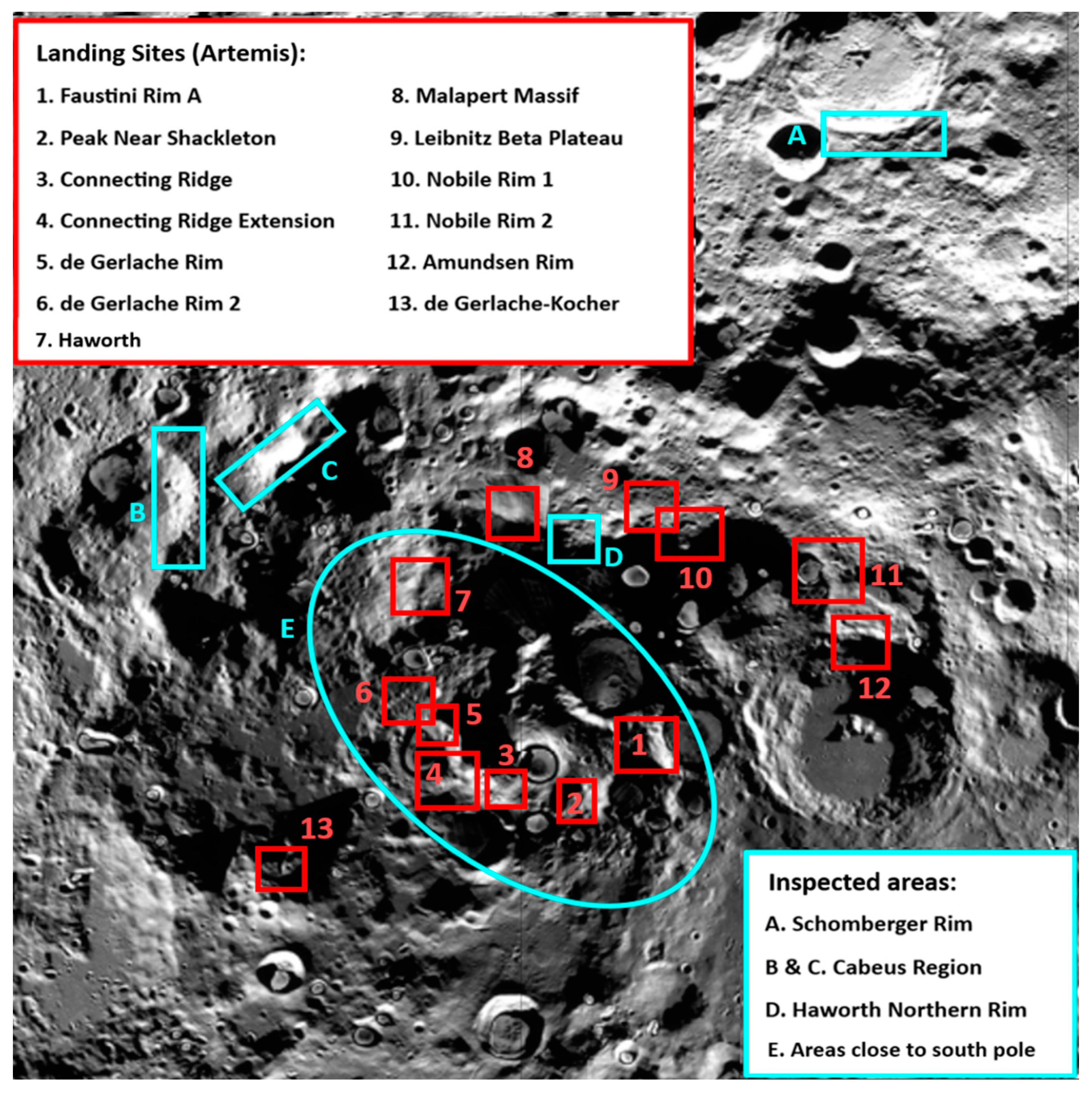
2.3. Candidate Locations for Future Lunar Settlements

The choice of the possible future landing and exploration sites on the lunar south pole is not an easy task and requires a careful analysis between aspects. Regions of interest (ROIs) should be located near permanently shadowed regions, offer a long duration of access to sunlight, direct-to-Earth communication and a surface slope and roughness favorable for landers and astronauts. Topographically high crater rims exposed to almost constant sunlight and located near these unilluminated crater floors seem to be the best location due to their proximity to potential vital resources and areas exploitable for solar power installations. Refs. [17,23] have proposed a series of main drivers in the selection of possible ROIs in the vicinity of the lunar south pole and they are combined in the following list:

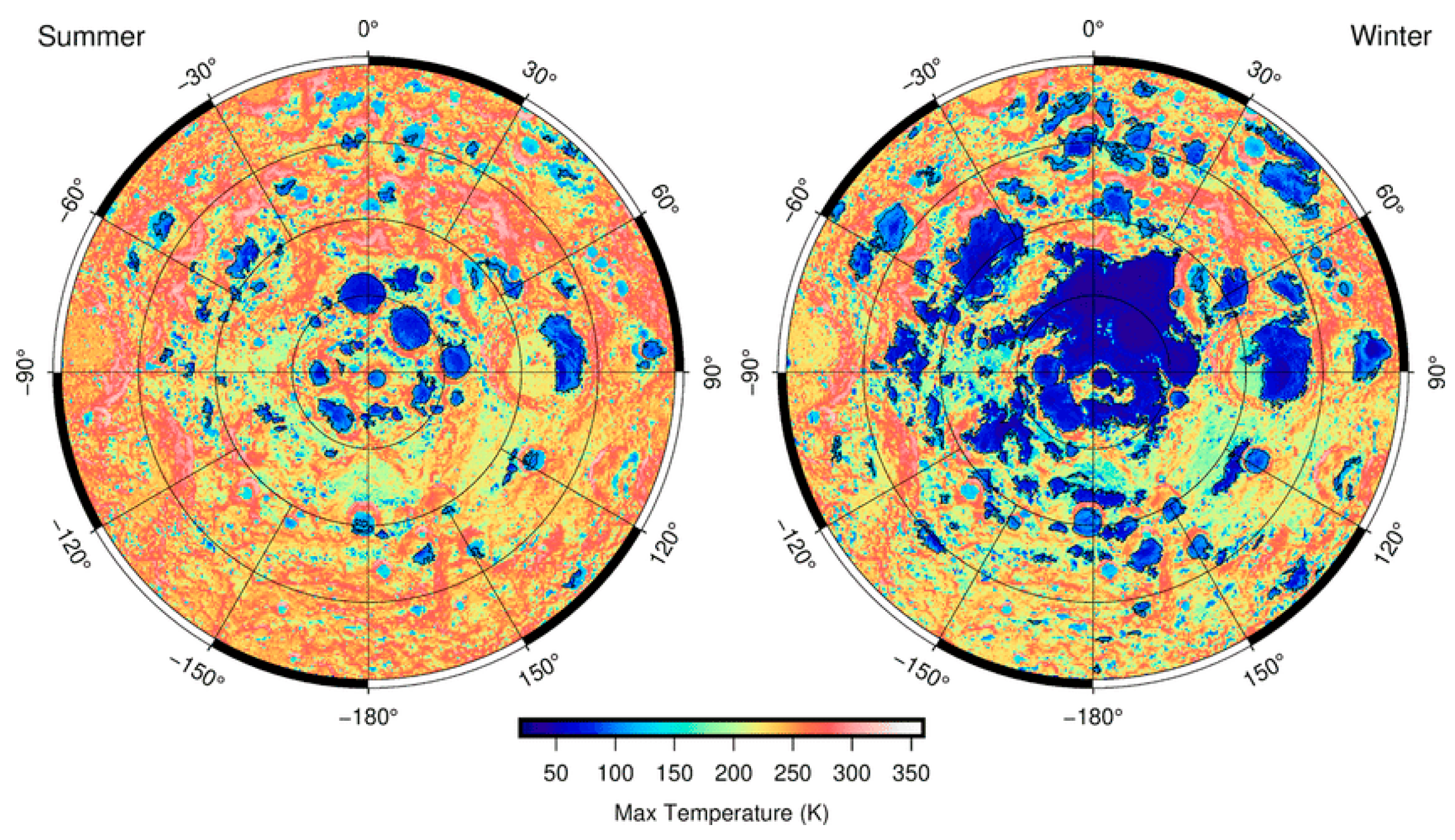
• The availability of water. In particular, a Diviner average temperature lower than 110 K. In this way, water ice is supposed to be stable at the surface and enhanced H signatures > 100 ppm by weight so ice should be present close to the surface; this last value derives from the LPNS, where a lower value means that the presence of water ice might be located deeper and so be harder to reach.
• The slopes of the terrain should be less than 20°. Based on the state of the art, lunar mission slopes greater than 15° can lead to the overturn of a lander while slopes up to 20° could guarantee safer extra vehicular activities.
• Usable energy source. Regions with a relatively higher average solar illumination (>50% of the lunar day) for power generation by solar panels.
• Communication link. Semi-continuous visibility of Earth is essential for the remote control of robotic operations and crew safety during the initial phase of lunar exploration programs when relay communication infrastructures will not yet be implemented.
• The base site should have enough areas for regular support ground operations and expansion (e.g., extra vehicular activities, EVAs)
• Abundance of mineral resources.
• Scientific interest to deepen the origin of our natural satellite.

Clearly, the most binding driver is that related to illumination, which largely impacts the design and duration of a mission considering that existing datasets suggest that there are no flat areas > 1 km² with illumination > 50% at latitudes > 80°. Despite everything, a tradeoff is necessary and the Artemis program has proposed 13 potential candidate sites, as shown in Figure 5. Accurate geodetic coordinates of each potential landing site can be accessed through NASA’s Moon Trek software [24].

Robotic missions scheduled for the next few years will surely pave the way to make the best choice among them.

3. Spectroscopic Survey

In the previous section, we have learned how spectroscopy constitutes a fundamental instrument to provide useful information about the lunar surface features. Spectroscopy is not always feasible with a dedicated mission due to the complexity of managing the cislunar space and the high cost; however, it is possible to implement it from Earth with the appropriate premises and the right expedients reducing the cost and increasing the ease of intervention. Most spectra found in the literature are taken in a wide spectral range, generally from the infrared region [15]; for this reason, the idea of performing an in-depth spectroscopy analysis of the lunar south pole with the Galileo Telescope (Asiago Astrophysical Observatory of the University of Padua) came up. The principal aim is to provide a detailed overview of the chosen region for future lunar settlements with the hope of enriching knowledge on the lunar environment.

3.1. The Galileo Telescope and Its Instrumentation

The telescope at the Asiago Astrophysical Observatory with its 122 cm primary mirror was constructed by “Officine Galileo” in Florence between 1940 and 1942 and dedicated to Galileo Galilei on the third centenary of his death. It is used in the Cassegrain configuration with a hyperbolic secondary mirror with a diameter of 52 cm. Since 1998, a Boller & Chivens spectrograph has been permanently mounted at the Cassegrain focus. It was manufactured by Perkin Elmer (model 58770). The B&C spectrograph features a slit at the Cassegrain focal plane with a variable aperture of up to 1 mm and a length of 28 mm. The collimator for directing the optical beam to the grating is an off-axis parabolic mirror with a diameter of 90 mm and a focal length of 810 mm. A set of four gratings with dispersion ranging from 42 Å/mm to 339 Å/mm complete the equipment of the spectrograph (

Table 1. Different gratings available for the Boller & Chivens spectrograph at the Galileo Telescope.

Denomination	Lines/mm	Blaze Wavelength [Å]	Spectral Range [Å]
300	300	5000	3500–7000
1200 R	1200	6825	5750–7000
600 V	600	4500	4250–6590
1200 B	1200	4000	3820–5020

). The dispersed light beam is directed towards the Dioptric Blue Galileo Camera with a focal length of 188 mm, and it operates in conjunction with an Andor iDus DU440 CCD camera with a sensor of 2048 × 512 pixels. The spatial resolution on the CCD is 1″/pixel. Several comparison lamps are permanently installed to enable wavelength calibration of the spectra. The side of the slit facing the incoming light beam has a reflective surface. On this surface, the image produced by the telescope is reflected to be captured by the guide camera (Andor iXon DV885 with an EMCCD sensor); the field of view is 8.5′ × 6.4′ with a resolution of 0.68″/pixel. A resume of the Galileo Telescope technical data can be found on

Table 2. The Galileo Telescope’s main technical features.

Longitude	E 11°31′35.138″
Latitude	N 45°51′59.340″
Altitude	1044.2 m above sea level
International code IAU-MPC	043
Primary mirror diameter (outer edge)	1237 mm
Primary mirror effective diameter	1200 mm
Primary mirror thickness (at the edge)	208 mm
Primary mirror focal length	6000 mm
Primary mirror focal ratio	f/5.0
Secondary mirror diameter	520 mm
Equivalent focal length	12,100 mm
Focal ratio	f/10.1
Scale	17.05 arcsec/mm

. The telescope is based on an English equatorial mounting and values are related to the intersection between its polar axis and declination axis.

3.2. Reduction of the Data Obtained with the Galileo Telescope

The “longslit” spectroscopy consists of passing light from an astronomical source through a thin rectangular aperture. A CCD sensor records the light diffracted by a scattering element, the grating. However, the data reduction needs other images for calibration in addition to those of the objects: bias, flat-field (quartz), caliber lamp (e.g., He-Fe-Ar) and spectrum of an any class spectro-photometric star (e.g., Vega, HR153, etc.; this procedure is necessary because the CCD response is measured in counts called ADU(x,y) (Analog Digital Units), which are related to the intrinsic signal of the plane of the sky I(x,y) by the relation:

ADU(x,y) = I(x,y)FF(x,y) + BIAS(x,y) + DARK(x,y) + SKY

(1)

where

• The BIAS(x,y) is obtained with the shutter closed and an exposure time of 0 s, i.e., 0 photoelectrons collected; in this way, subtracting photo-electrons from the scientific image countings due to instrumental effects are eliminated.
• The flat-field FF(x,y) is obtained by pointing the telescope towards the closed dome illuminated by the uniform light from a lamp (this method is also known as dome flat). Thus, the obtained spectrum is composed of the continuum spectrum from the lamp, the response curve of the CCD and the non-uniform pixel response.
• The DARK(x,y) is due to the eddy currents that are generated in the CCD caused by thermal agitation. This contribution can be neglected because modern CCDs are kept at very low temperatures (−80/90 °C).
• Other images used are those of the He-Fe-Ar lamp and the standard star, respectively, for the wavelength calibration and the flux calibration.

The reduction of the spectra has been made with the IRAF (Image Reduction and Analysis Facility), which allows processing astronomical images; in our specific case, the Pennar pipeline made available by the observatory of Asiago has been used.

Solar Analogs

The Moon is not bright due to proper light but it reflects the one coming from the Sun. Therefore, it is necessary to have a reference spectrum of the Sun and then divide the Moon spectrum by this reference one. The reference spectrum is chosen from a list of the so-called solar analogs (stars belonging to the same spectral class of the Sun); as in the case of the spectro-photometric standard star, the choice falls on the one with the coordinates as close as possible to the Moon in order to improve the air mass corrections. A detailed list of the solar analogs is reported in

Table 3. Typical stars defined as solar analogs (same spectral class of the Sun) used as the divisor in the reduction of “relative flux” spectra.

Star	RA [hh mm ss]	Dec [° ′ ″]	V Mag
Land (SA) 93–101	01 53 18.0	+00 22 25	9.7
Hyades 64	04 26 40.1	+16 44 49	8.1
Land (SA) 98–978	06 51 34.0	−00 11 33	10.5
Land (SA) 102–1081	10 57 04.4	−00 13 12	9.9
Landolt (SA) 107–684	15 37 18.1	−00 09 50	8.4
Land (SA) 107–998	15 38 16.4	+00 15 23	10.4
16 Cyg B	19 41 52.0	+50 31 03	6.2
Land (SA) 112–1333	20 43 11.8	+00 26 15	10.0
Land (SA) 115–271	23 42 41.8	+00 45 14	9.7

. To compare all the spectra from different night observations, the solar analog flux is normalized to its peak of flux emission, in a range where the continuum is regular and without pronounced absorptions. The normalization takes place at various wavelengths depending on the used grating: 5500 Å for the 300 lines and the 600 V, 6000 Å for the 1200 R and 4150 Å for the 1200 B. The spectra of Hyades 64 and 16 Cygni B have been used during this survey. The solar analog is usually taken before the observation of the selected object because if the weather becomes worse, the risk of losing all the collected data becomes high.

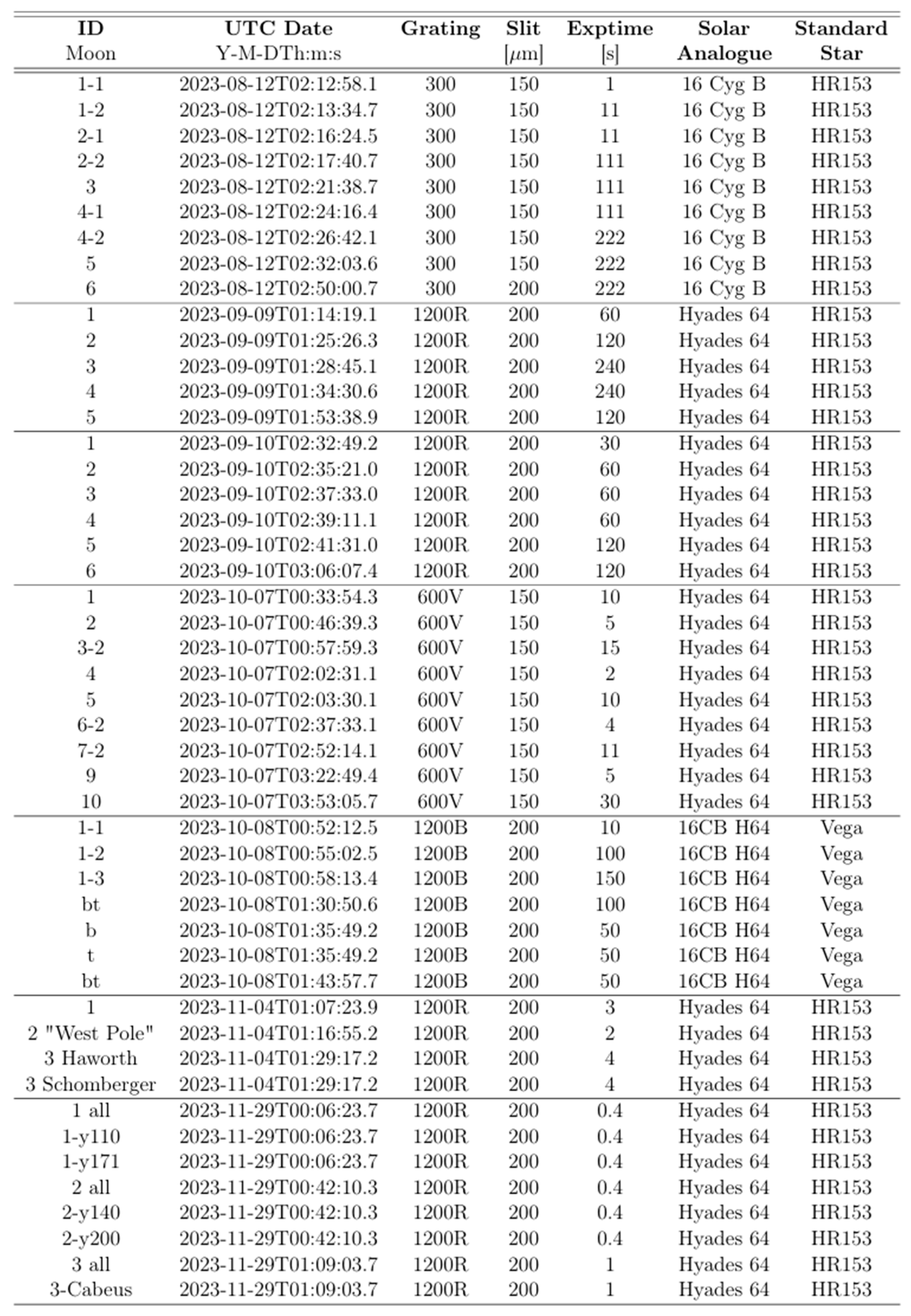
3.3. Observing Campaign

Observing the Moon with the Galileo Telescope is not trivial; the telescope is designed to observe faint objects. There are some issues to deal with and to focus on, which will be outlined below as follows:

• The Moon’s brightness is the first relevant driver. To avoid saturation of the image, the exposure time needs to be properly reduced. The saturation occurs when the countings exceed this value 2^nbit, i.e., 65,536 counts; however, the sensor loses linearity beyond 40,000 counts while under 30,000 counts, the signal to noise ratio (SNR) increases.
• Exposure time below the second might give rise to some errors due to the calibration of the mechanical shutter being set on poses of several minutes. During a full Moon, it is necessary to act on the diaphragm aperture, which has to be rightly closed to minimize faults that affect the flux results and to extend the exposure time; because of this, a good spatial resolution for the guide camera could be lost.
• The Moon’s proximity to the Earth causes a rapid variation in the Moon’s coordinates, and robotically or differential tracking are not possible; for example, the Schimdt (the robotic telescope of the INAF Astronomic Observatory of Padua), in addition to not pointing at the Moon, cannot even approach it. Nonetheless, the Galileo Telescope has the ability to perform manual tracking at three different speeds; in this way, we can follow the Moon’s motion seamlessly and we have freedom of choice in the observable areas. This is not a common feature but thanks to that, the tracking of the selected bright zone has been performed in a meticulous way.
• The guide camera does not have a high resolution due to air turbulence and it works poorly in a high illumination condition; so, positioning the slit on the right zone and navigating on the lunar surface is not always an easy issue. This phenomenon of image distortion is augmented when approaching polar latitudes due to the Moon’s sphericity.
• Another important aspect is bound up with the subtraction of the sky’s emission. This operation can be performed in different positions depending on the objective of the observations; in most instances, a compromise is necessary. For example, the Moon has an exosphere up to 500 km thick, which does not need to be considered for a lunar surface spectroscopy analysis. This is ensured by the length of the slit (8.5 arcminutes on the celestial plane, about 950 km of field of view in width) that allows extracting the lines of the sky without “contaminating” the final spectrum.

Moreover, it is necessary to bear in mind that not all of the Moon’s visible area can be analyzed due to the apparent diameter of the Moon but the “longslit” spectroscopy makes all the observations near the Moon’s edge or terminator easier. As emerged in the last sentence, the terminator reveals a more observable area and so the better nights are not the ones with the full Moon but those during the waxing descent or crescent phase, even it could seem counter intuitive; Figure 6 gives a better comprehension of this concept. During a full Moon, the slit (depicted with lines of different colors) can be positioned only tangentially to the edge, as evidenced by the middle image. On the other hand, the right and left images highlight how a crescent or descent phase offer a wider range of positioning possibilities; nevertheless, a certain degree of contamination by the lunar exosphere has to be taken into account when observing bright zones along the terminator. The ideal condition would be with the Moon in its crescent or descent phase, a low value of air mass and the slit positioned in a parallactic way; obviously, the Moon’s ephemerides do not ensure all these conditions and a tradeoff is required.

• The back-illuminated ANDOR sensor provides an excellent performance in ultraviolet, while suffering from fringing (photons interference) in the near-infrared due to sensor thinning. All the spectra presented hereafter are aptly cut in the way of not displaying the wavelength where this phenomenon occurs.
• Unfortunately, it is not possible to make many observations; only two or three nights per month with a favorable libration are exploitable. Our principal constraint is the libration in latitude, which results in a modest inclination (an average of 6.7° in modulus) between the Moon’s axis of rotation and the normal to the plane of its orbit around Earth; Galileo Galilei was sometimes credited with the discovery of this specific lunar motion. The slightest value of libration makes the lunar south pole visible for an observer on Earth. This kind of lunar motion is simplified in Figure 7 to make understanding more intuitive. The lunar ephemeris has been obtained from [25].
• Lastly, such a detailed spectroscopy survey of the Moon has never been made with the Galileo Telescope and so several attempts were required.

3.4. Results

In this subsection will be presented some of the most significant spectra obtained during this observation campaign with a brief analysis of what they provide. As previously highlighted, all the lunar south pole spectra fluxed thanks to the spectrophotometric star are divided by their respective normalized solar analog; this provides a series of diagrams with ”Absolute flux” on the y-axis. This step is not negligible because it makes results from different nights comparable. For the purpose of a correct interpretation of the spectra, it is essential to specify that the emission lines (atoms) or bands (molecules) are derived only from gas that is optically thin while absorptions could derive from gas that is optically thick or solid-state elements; consequently, through the emissions, it is possible to observe the Moon’s soil features indirectly. Meanwhile, the continuum slope color derives only from a solid-state element. Lastly, Figure A1 provides a complete catalog of the observations pointing out when and with which set up they were carried out.

3.4.1. Grating: 300

The first observations have been conducted by sacrificing resolution but favoring a wide spectral range. Figure 8 encloses some of the spectra obtained where the first characteristic features become observable. The K and H of calcium emissions appear clearly visible at ~3935 Å and ~3970 Å, respectively; these wavelengths are well known in the solar spectrum, and they will be described subsequently. Another manifest feature is specified with a red arrow in Figure 8; every spectrum shows this distinctive trend in the correspondence of the Na doublet wavelength (~5890 Å). It could not be compensated with the solar analog and so it has driven us to deeply investigate this direction with a more defined grating. As stated before, sodium is an important volatile and it may be related to the presence of water; a strong emission of Na has been observed on the lunar impact plume immediately after the LCROSS event towards the Cabeus crater, one of the craters richest in water of the lunar south pole [20].

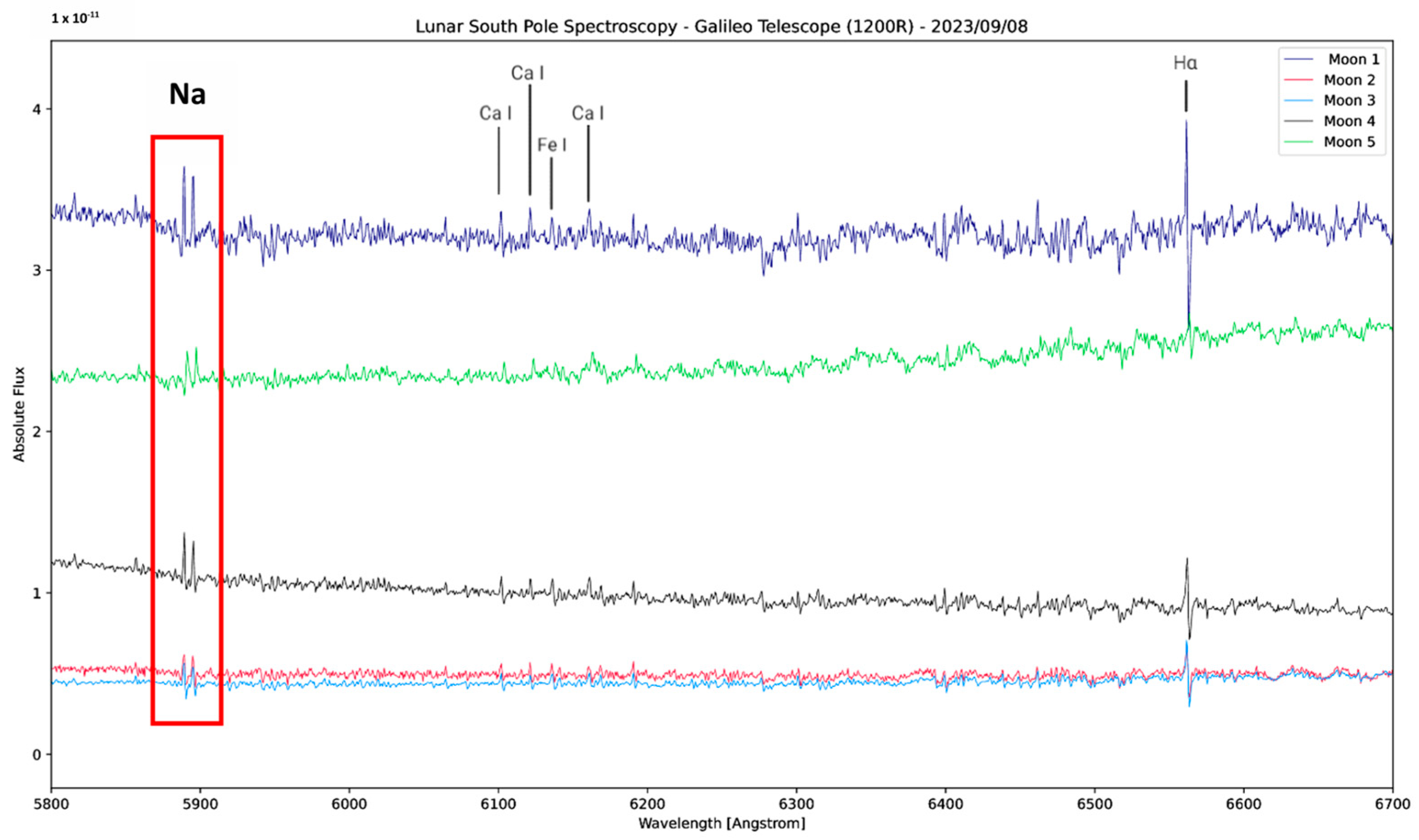
3.4.2. Grating: 1200 R

The enhanced resolution confirms the presence of the Na doublet whose peaks at 5889 Å and 5895 Å are clearly distinct; the results of other emissions of Ca I (6102.4 Å, 6122 Å, 6161.5 Å) and Fe I (6136.7 Å) are well visible, as shown in Figure 9. An interesting analysis with this grating was carried out in November 2023. The position of the lunar terminator allowed having both the bright rims of Haworth (PSR) and Schomberger craters inside the slit simultaneously; in this way, it has been possible to divide the two spectra. This is an important aspect because the two spectra have been obtained and reduced likewise, so their ratio may furnish extremely reliable data. The “Haworth/Schomberger” spectrum underlines that the sodium emission intensity is higher for the Haworth crater. Only if the sky subtraction has been made in the same manner is it possible to exclude that the emission derived from the lunar exosphere may arise from other causes, which highlights differences between the two areas.

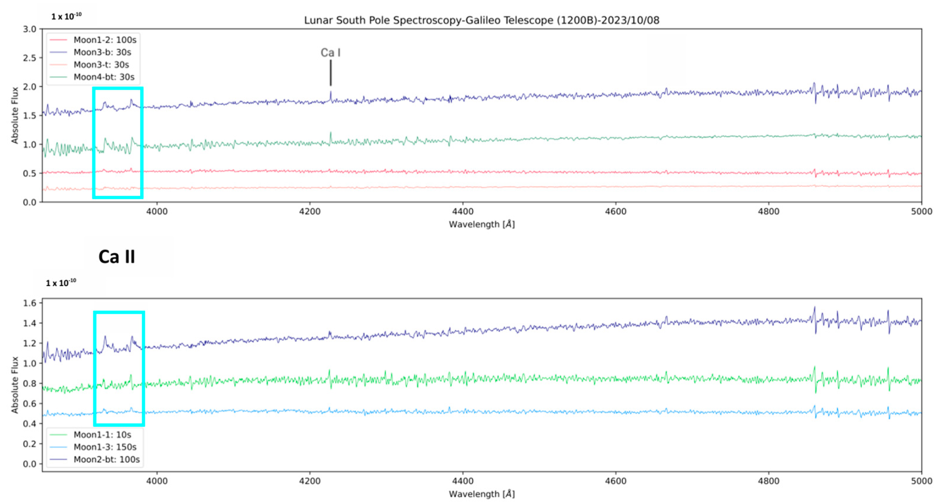
3.4.3. Grating: 1200 B

The spectra obtained with this grating do not reveal particular features useful to enrich the lunar surface description, but they might give us information on the solar activity. As said previously, typical emissions of the solar spectrum are H and K of calcium and Figure 10 points out how strong they are. During these days, the Sun was very active, and the solar chromosphere is more in emission than usual; one of the characteristic chromosphere emissions is precisely that of calcium. In this way, it may be possible to track the solar activity during night and this constitutes the only way to monitor the Sun from the Asiago Astrophysical Observatory.

3.4.4. Grating: 600 V

Observation with the 600 V grating highlights another strong emission. Within the wavelength range 5165–5185 Å, the magnesium triplet is clearly visible in all the spectra, as seen in Figure 11; it could be interesting to understand the origin of this emission, in particular if it could be derived from a salt dissociation. Furthermore, the sodium doublet emission appears less pronounced, but the two characteristic peaks remain distinct. Emissions of Ca are present at 6160 Å and 6169 Å while there is Fe emission at 4984 Å and 4385 Å. Ultimately, some spectra reveal a conspicuous emission of CH.

4. Discussion

The obtained results provide a unique overview of the lunar south pole surface spectroscopy in the visible spectral range with all the available gratings from the Boller & Chivens spectrograph. Moreover, it was the first survey of this type performed by the Galileo Telescope of the Asiago Astrophysical Observatory. As evidenced in the previous chapter, finalized spectroscopy analysis for water detection has been performed beyond 10,000 Å, an example can be found in ref. [26]; finding a correlation with the visible presence of water also gives another perspective to water abundance on the lunar surface. During this spectroscopic survey, sodium has been indicated as one of the characteristic emissions. This emission is particularly recurring between certain celestial bodies, and it could be interesting to investigate whether it may have a common origin through joint observations. Two attempts to characterize the sodium Mercury tail were carried out in March and July 2024 but the weather conditions were not favorable, especially due to the high reverberation generated by sunlight. Further comparisons may be proceeded towards some asteroids, and a good candidate could be Ceres, or Callisto, one of the natural moons of Jupiter. For example, the latest analyses on the fragments of the asteroid Bennu have revealed the presence of sodium and magnesium phosphate [27]. Either way, an additional hypothesis and a more detailed analysis of the spectra will be possible once inspected by lunar geology and exosphere experts. This spectroscopic survey is meant to represent only a first iteration, and improvements in the observational procedures and instrumentation can be carried out; for example, the purchase of a new thick sensor is scheduled to improve the resolution in NIR and avoid the fringing phenomenon. Once spectral regions with interesting features are found, it could be useful to investigate with a higher resolution through an Echelle-type spectroscopy.

In conclusion, to answer the question “Why performing such a survey with a telescope from Earth?”, a series of strong points will be presented below as follows:

• Flexibility in the set up and observational procedure;
• Quick access to the astronomic observatory structures;
• Rapid intervention. In the case of out-of-the-ordinary phenomena, it is possible to observe almost in real time. An example could be the dust plume that arose from the crash of a spacecraft on the lunar surface as happened with the private Japanese Hakuto-R Mission 1 in April 2023, the Roscosmos mission Luna 25 in August 2023 or how it could have happened with the Peregrine lander in January 2024. Events of this nature can offer great opportunities to study the lunar surface in an unusual way.
• The possibility of following from beginning to end the observational procedure and obtaining “own measurements”. This is one of the most important points because the observer knows how he obtained those results and, in case of need, he can improve or modify them.

5. Conclusions

This work is not only intended to provide input to the research of and improvement in Earth-based spectroscopic investigations, but also to be a good starting point for the development of orbital- and lunar-based infrastructures to ensure proper coverage and support to these regions of interest. In fact, a second work is being prepared, which relies on the results obtained in this part aimed at developing a satellite constellation to provide 24 h coverage of the lunar south pole.

References

1. Bhamidipati, S.; Mina, T.; Sanchez, A.; Gao, G. Satellite Constellation De sign for a Lunar Navigation and Communication System. NAVIGATION J. Inst. Navig. 2023, 70, navi.613. [Google Scholar]
2. The International Space Exploration Coordination Group. Available online: https://www.globalspaceexploration.org (accessed on 12 July 2024).
3. Ouyang, Z.Y. Cosmochemistry; Beijing Science Press: Beijing, China, 1989; Volume 93. [Google Scholar]
4. Zou, Y.L.; Liu, J.Z.; Liu, J.J.; Xu, T. Reflectance spectral characteristics of Lunar surface materials. Chin. J. Astron. Astrophys. 2004, 4, 97. [Google Scholar] [CrossRef]
5. Crawford, I.A. Lunar resources: A review. Prog. Phys. Geogr. 2015, 39, 137–167. [Google Scholar] [CrossRef]
6. Ambrose, W.A.; Cutright, B.L. Water Ice Resources on the Moon; Gulf Coast Association of Geological Societies Transactions: Nacogdoches, TX, USA, 2023; Volume 72, pp. 231–241. [Google Scholar]
7. Spudis, P.D.; Gillis, J.J.; Reisse, R.A. Ancient multiring basins on the Moon revealed by Clementine laser altimetry. Science 1994, 266, 1848–1851. [Google Scholar] [CrossRef] [PubMed]
8. Unified Geologic Map of the Moon. Available online: https://astrogeology.usgs.gov/search/map/Moon/Geology/Unified_Geologic_Map_of_the_Moon_GIS_v2 (accessed on 12 July 2024).
9. Mazarico, E.; Neumann, G.A.; Smith, D.E.; Zuber, M.T.; Torrence, M.H. Illumination conditions of the lunar polar regions using LOLA topography. Icarus 2011, 211, 1066–1081. [Google Scholar] [CrossRef]
10. Lunar South Pole Atlas. Available online: https://www.lpi.usra.edu/lunar/lunar-south-pole-atlas/ (accessed on 12 July 2024).
11. O’Brien, P.; Byrne, S. Mapping Lunar Double Shadows with Digital Terrain Models. LPI Contrib. 2022, 2703, 5012. [Google Scholar]
12. Mahanti, P.; Robinson, M.S.; Wagner, R.; Estes, N.; Humm, D.C. First Look, First Results-Comparing Secondary Illumination at Lunar Permanently Shadowed Regions from the First Shadowcam Image and Topography Based Simulation. In Proceedings of the IGARSS 2023-2023 IEEE International Geoscience and Remote Sensing Symposium, Pasadena, CA, USA, 16–21 July 2023; IEEE: Piscataway, NJ, USA, 2023; pp. 4162–4165. [Google Scholar]
13. Moriarty, D.P.; Watkins, R.N.; Petro, N.E. Mineralogical diversity of the lunar south pole: Critical context for artemis sample return goals and interpretation. In Proceedings of the Lunar Surface Science Workshop, Virtual, 28–29 May 2020; Volume 2241, p. 5152. [Google Scholar]
14. Wu, Y.; Hapke, B. Spectroscopic observations of the Moon at the lunar surface. Earth Planet. Sci. Lett. 2018, 484, 145–153. [Google Scholar] [CrossRef]
15. Li, S.; Lucey, P.G.; Milliken, R.E.; Hayne, P.O.; Fisher, E.; Williams, J.P.; Hurley, D.M.; Elphic, R.C. Direct evidence of surface exposed water ice in the lunar polar regions. Proc. Natl. Acad. Sci. USA 2018, 115, 8907–8912. [Google Scholar] [CrossRef]
16. Hurley, D.; Colaprete, A.; Elphic, R.; Farrell, W.; Hayne, P.; Heldmann, J.; Hibbitts, C.A.; Hurley, D.M.; Livengood, T.A.; Sherwood, B.; et al. Lunar Polar Volatiles: Assessment of Existing Observations for Exploration; NASA Goddard Space Flight Center: Greenbelt, MD, USA, 2016.
17. Flahaut, J.; Carpenter, J.; Williams, J.P.; Anand, M.; Crawford, I.A.; van Westrenen, W.; Füri, E.; Xiao, L.; Zhao, S. Regions of interest (ROI) for future exploration missions to the lunar South Pole. Planet. Space Sci. 2020, 180, 104750. [Google Scholar] [CrossRef]
18. Livengood, T.A.; Chin, G.; Boynton, W.; McClanahan, T.P.; Su, J.J. Latitude Dependence of the Hydrogen/Water Concentration in the Lunar Surface Measured by LRO/LEND. In AAS/Division for Planetary Sciences Meeting Abstracts; American Astronomical Society: Washington, DC, USA, 2022; Volume 54, p. 316.04. [Google Scholar]
19. Killen, R.M.; Potter, A.E.; Hurley, D.M.; Plymate, C.; Naidu, S. Observations of the lunar impact plume from the LCROSS event. Geophys. Res. Lett. 2010, 37. [Google Scholar] [CrossRef]
20. Heldmann, J.L.; Lamb, J.; Asturias, D.; Colaprete, A.; Goldstein, D.B.; Trafton, L.M.; Varghese, P.L. Evolution of the dust and water ice plume components as observed by the LCROSS visible camera and UV–visible spectrometer. Icarus 2015, 254, 262–275. [Google Scholar] [CrossRef]
21. de Castro, N.W.; Li, S. Characterizing Spectral Features of Water-ice, Lunar Regolith Simulants, and their Mixtures at the VIS-NIR Region. LPI Contrib. 2022, 2703, 5035. [Google Scholar]
22. Sanin, A.B.; Mitrofanov, I.G.; Litvak, M.L.; Bakhtin, B.N.; Bodnarik, J.G.; Boynton, W.V.; Vostrukhin, A.A. Hydrogen distribution in the lunar polar regions. Icarus 2017, 283, 20–30. [Google Scholar] [CrossRef]
23. Leone, G.; Ahrens, C.; Korteniemi, J.; Gasparri, D.; Kereszturi, A.; Martynov, A.; Schmidt, G.W.; Calabrese, G.; Joutsenvaara, J. Sverdrup-Henson crater: A candidate location for the first lunar South Pole settlement. Iscience 2023, 26, 107853. [Google Scholar] [CrossRef] [PubMed]
24. Moon Trek. Available online: https://trek.nasa.gov/moon/index.html#v=0.1&x=0&y=0&z=1&p=urn%3Aogc%3Adef%3Acrs%3AEPSG%3A%3A104903&d=&locale=&b=moon&e=-300.05858815283705%2C-157.85155955550536%2C300.05858815283705%2C157.85155955550536&sfz=&w= (accessed on 12 July 2024).
25. Geocentric Ephemeris for the Moon. Available online: https://astropixel.com/ephemeris/moon.html (accessed on 12 July 2024).
26. Lemelin, M.; Camon, A.; Li, S.; Diotte, F.; Lucey, P.G. Water Ice Detections in the Polar Regions using the Kaguya Spectral Profiler. LPI Contrib. 2022, 2703, 5039. [Google Scholar]
27. Lauretta, D.S.; Connolly, H.C., Jr.; Aebersold, J.E.; Alexander, C.M.O.D.; Ballouz, R.L.; Barnes, J.J.; Bates, H.C.; Bennett, C.A.; Blanche, L.; OSIRIS-REx Sample Analysis Team; et al. Asteroid (101955) Bennu in the laboratory: Properties of the sample collected by OSIRIS-REx. Meteorit. Planet. Sci. 2024. [Google Scholar] [CrossRef]
Figure 1. Maps of the lunar south pole (80° to pole) derived from the Lunar Reconnaissance Orbiter (LRO) Lunar Orbiter Laser Altimeter (LOLA). (a) Topographic and slope maps adapted from [10], (b) Earth visibility and solar illumination maps of the lunar south pole adapted from [9].
Aerospace 11 00693 g001
Figure 2. Summer and winter lunar south pole surface maximum temperature. A black demarcation line for 110 K defines the approximate threshold value for PSRs (adapted from [9]).
Aerospace 11 00693 g002
Figure 3. Elemental abundances of iron, potassium, thorium and titanium in the lunar south pole detected with the Lunar Prospector instruments, adapted from [13].
Aerospace 11 00693 g003
Figure 4. From left to right: location of the permanently shadowed regions [10] and distribution of water-equivalent hydrogen (WEH) around the lunar south pole. The second image also highlights the first eight areas for the abundance of WEH (adapted from [22]); the first one corresponds to the Cabeus crater.
Aerospace 11 00693 g004
Figure 5. The NASA’s Artemis 13 candidate landing sites (red) and the observed areas during the spectroscopic survey (cyan). The background image of the lunar south pole (80°S to pole) is from the Lunar Reconnaissance Orbiter’s wide-angle Camera, adapted from [10].
Aerospace 11 00693 g005
Figure 6. This triptych of images shows different possibilities for positioning the slit during distinct Moon phases.
Aerospace 11 00693 g006
Figure 7. Illustration of the libration in latitude.
Aerospace 11 00693 g007
Figure 8. Spectra of the lunar south pole with the 300 lines grating. Every spectrum corresponds to a different bright area. Two noticeable features are pointed out: the H and K of Ca emission and the area close by the Na doublet with its typical trend pointed out with red arrows. For the legend, see Appendix A. From the 1.22 m Galileo Telescope 12/08/2023.
Aerospace 11 00693 g008
Figure 9. Spectra of the lunar south pole with the 1200 R grating. The most evident emissions arise from the Na doublet; other minor emissions are from Ca I and Fe I. For the legend, see Appendix A. From the 1.22 m Galileo Telescope 09/09/2023.
Aerospace 11 00693 g009
Figure 10. Spectra of the lunar south pole with the 1200 B grating. The H and K of calcium emissions (highlighted in cyan) are the most significant and through their intensity the solar activity can be monitored during night. For the legend, see Appendix A. From the 1.22 m Galileo Telescope 08/10/2023.
Aerospace 11 00693 g010
Figure 11. Spectra of the lunar south pole with the 600 V grating. The most characteristic emission is from the magnesium triplets (highlighted in green). Other typical emissions derive from calcium, iron and hydrogen. For the legend, see Appendix A. From the 1.22 m Galileo Telescope 07/10/2023.
Aerospace 11 00693 g011