Lessons Learnt from the Simulations of Aero-Engine Ground Vortex

Abstract

With the startup of the aero-engine, the ground vortex is formed between the ground and the engine intake. The ground vortex leads to total pressure and swirl distortion, which reduces the performance of the engine. The inhalation of the dust and debris through a ground vortex can erode the fan blade, block the seals and degrade turbine cooling performance. As the diameter of the modern fan blade becomes larger, the clearance between the intake lip and the ground surface is smaller, which enhances the strength of the ground vortex. Though considerable numerical studies have been conducted with the predictions of the ground vortex, it is noted that the accurate simulation of the ground vortex is still a tough task. This paper presents authors’ simulation work of the ground vortex into an intake model with different crosswind speeds. This paper tackles the challenge with a parametric study to provide useful guidelines on how to obtain a good match with the experimental data. The influence of the mesh density, performance of different turbulence models and how the boundary layer thickness affects the prediction results are conducted and analysed. The detailed structure of the flow field with ground vortex is presented, which can shed light on the experimental observations. A number of suggestions are presented that can pave the road to the accurate flow field simulations with strong vorticities.

1. Introduction

Modern underwing podded engines have higher bypass ratios and fan blades with larger diameters, which lead to a shorter distance between the intake and the ground. Ground vortex can be formed under quiescent, headwind and crosswind conditions [1]. The ingested ground vortex promotes the generation of the total pressure distortion and swirl distortion into the engine, which can reduce its surge margin [2,3]. The ground vortex will also lift foreign objects into the engine, which may lead to the wear of the fan blade, erosion of the compressor blades and seals or degraded turbine cooling performance. It may also cause the vibration of the fan blade [4,5]. The operation of the intake in crosswind conditions can lead to the formation of the vortex with particular strength, which is primarily determined by the velocity ratio ($U_i/U_{\infty }$, the ratio between the average inlet flow velocity and the crosswind velocity) and the normalised ground clearance (the vertical distance from the lowest point of the highlight plane to the ground, $h$, normalised by the intake highlight diameter, $D_l$). Lip separation can also occur when the crosswind is strong. Therefore, the operation in crosswind is considered as one of the most severe conditions of the engine intake.

To understand the formation and the behaviour of the ground vortex, numerous studies have been conducted [6,7,8,9,10,11,12,13]. Previous studies have also investigated and proposed the criterion to judge whether the ground vortex will exist for different flow conditions such as crosswind speeds and ground clearances [2,9,13,14]. The active control or suppression of the ground vortex has been reviewed in [10,15]. Recently, the blowing away process of the ground vortex has been investigated experimentally in [16].

To facilitate the prediction of the behaviour of the ground vortex, the computational fluid dynamic (CFD) simulations have been increasingly adopted [3,15,17,18,19,20,21]. These studies contributed to the analysis of the flow field structure with the ground vortex and provided valuable details as the three-dimensional visualisation of the ground vortex is demanding and costly. However, in most instances, the numerical simulations can only deliver qualitative estimations while the accurate prediction of the behaviour of the ground vortex is still very challenging [22,23]. For the simulations with low-speed crosswinds and low-speed inflow velocity, the match between the CFD and the experimental data is generally good. The simulations of the ground vortex with the crosswind speed of 10 m/s and the intake speed of 85 m/s can display a good agreement with the measured data in terms of the vortex equivalent radius and vortex tangential velocity [20,24]. The large eddy simulation (LES) at low Re number ($5\times {10}^4$) performed in [19] can capture the observations in the experimental data [6] qualitatively. In another work [25], LES is used to study the dynamics of the ground vortex, and a comparison of the mean velocity field shows good agreement between the experimental and the CFD results. The mean velocity through the intake is 26 m/s, which results in a Reynolds number of about 65,000. The numerical study presented in [16] investigated the vortex behaviours with the intake suction speed up to 32 m/s and the crosswind velocity up to 14 m/s, and the intake Reynolds number ranged from 1.74 × 10⁵ to 2.18 × 10⁵.

The ground vortex study by Murphy [10] was selected as the test case in the fifth IAA Propulsion Aerodynamics Workshop (PAW5) in January 2021. The purpose of the workshop is to assess the accuracy of existing CFD codes in simulating the aerodynamic impact of the ground vortex. The simulated flow field was compared against the measured data in terms of the total pressure contour at the aerodynamic interface plane (AIP) and the three-component flow velocity near the ground surface. Generally, most solvers used during the workshop obtain a better match with the experimental data at low crosswind speeds, but the discrepancies between the CFD and test data are large for the conditions of higher crosswind speeds.

This paper aims to provide useful instructions for the accurate simulations of ground vortex by conducting a comprehensive parametric study. The influence of the mesh density, turbulence model and thickness of the boundary layer are investigated numerically. The simulated results are compared against the experimental data, and the influence of the numerical setup is discussed.

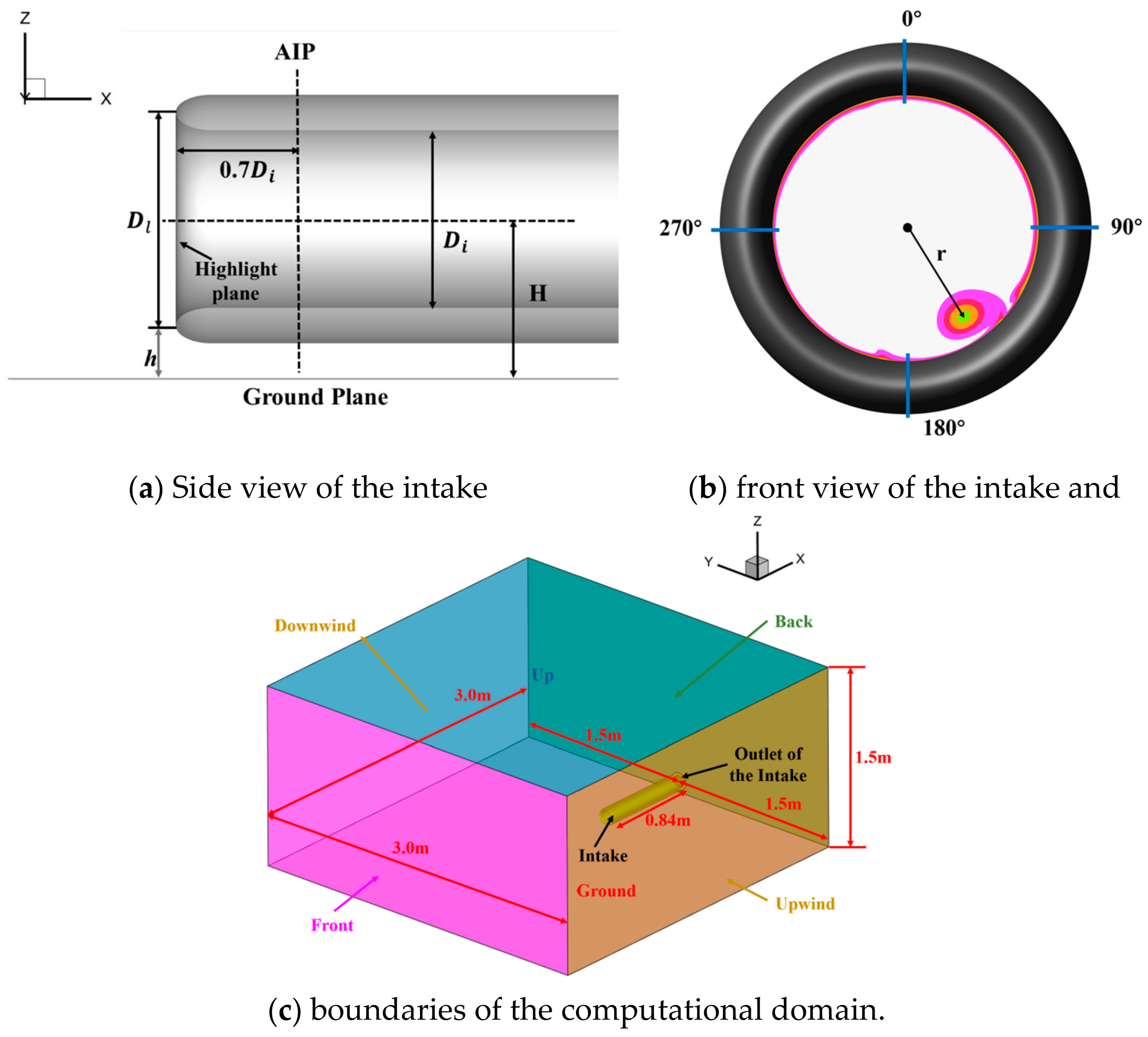
2. Case Setup

The ground vortex case supplied by the AIAA Propulsion Aerodynamic Workshop [26] is chosen in the current research. The experiments were carried out in the Cranfield University low-speed wind tunnel [10]. The working section of the wind tunnel is 2.4 m × 1.8 m. An axisymmetric and cylindrical intake model without any centre body is adopted in the experiments. The height of the lower lip is $h/D_l=0.25$. The inner diameter $D_i$ is 0.1 m, and the outer diameter $D_l$ is 0.12 m. The total pressure rakes inside the intake are placed at the AIP, which is 0.7 $D_i$ from the highlight plane. This is the nominal fan face location. The measurements include the total pressure at the AIP and the wall static pressure inside the intake, where the parameter may have the most important influence on the engine performance. Stereoscopic Particle Image Velocimetry (SPIV) is used to acquire the three components of the flow velocity (u, v, w) of the ground vortex in the plane, which is around 10 mm above the ground surface. The air speed in the working section can be adjusted from 10 m/s to 50 m/s. The thickness of the boundary layer in the test section is adjustable with the suction slots upstream of the intake. The intake is connected to a large vacuum tank through a shutter valve. The air is sucked into the intake once the shutter is opened. During the experiments with crosswind, the maximum mass flow is 1.46 kg/s and the intake Mach number is 0.55. Detailed introductions of the experimental approach and methodology can be found in [10].

The computational domain provided by the workshop committee is shown in Figure 1. One of the meshes provided by the workshop has 44 million cells composed of tetraheda, prisms, pyramids and hexahedra (named as Mesh A). The initial wall spacing of the intake surface and the ground plane is 1.27 × 10⁻³ mm and 6 × 10⁻³ mm, respectively. This ensures that the $y^{+}$ value is less than one for the first layer near wall mesh. The growth rate of the boundary layer mesh is 1.16. The grid is gradually coarsened in the regions away from the intake. More information about the grid can be found in [22]. The second one (named as Mesh B) is generated with a refinement for the region with ground vortex, which will be introduced later.

In the simulation, the crosswind enters the domain along the Y direction. The axial centreline of the intake is along X direction. To describe the location of vortex core at the AIP surface, the circumferential angle $\theta$ and the radius $r$ of the vortex core are defined in Figure 1c. In the test matrix, the mass flow through the intake is fixed and the amplitude of the crosswind is changed. In this study, four different crosswind velocities (Ui/U_∞ = 18.3, 9.2, 6.1 and 5.2) are simulated. The velocity profile at the upwind is defined as

$$U_y=U_{\infty }\times {(y/0.104)}^{1/8.28}.$$

The free stream total pressure and total temperature at the upwind surface in the domain are tabulated in

Table 1. Test matrix of the ground vortex simulation.

Case	Pt (Pa)	Tt (K)	${\mathit{U}}_{\mathit{\infty }}$ (m/s)	Ui/U∞	${\dot{\mathit{m}}}_{\mathit{i}}(\mathbf{k}\mathbf{g}/\mathbf{s})$
1	100,880	290	9.92	18.3	1.46
2	100,910	290	20.0	9.1	1.46
3	100,970	290	30.2	6.1	1.46
4	101,000	290	35.4	5.2	1.46
5	101,000	290	39.0	4.6	1.43
6	101,000	290	45.0	4.0	1.42

. The pressure-outlet boundary condition is used at the downwind surface to obtain the prescribed $U_{\infty }$ at the upwind surface. At the exit surface of the intake, the static pressure is adjusted to obtain the prescribed mass flow through the intake (1.46 kg/s). Unless otherwise specified, all the other surfaces of the domain are set as viscous adiabatic walls.

The solver used in this study is Ansys Fluent. An implicit, density-based scheme is used to solve the three-dimensional conservation equations as the maximum Mach number in the flow field can exceed 0.88. The continuity equation for mass conservation is given by

$${\displaystyle \frac{\partial \rho }{\partial t}}+\nabla ·\left(\rho \overrightarrow{u}\right)=0$$

where ρ is density, and $\overrightarrow{u}$ denotes the velocity. The momentum equation is described as

$${\displaystyle \frac{\partial \left(\rho \overrightarrow{u}\right)}{\partial t}}+\nabla ·\left(\rho \overrightarrow{u}\overrightarrow{u}\right)=-\nabla p+\nabla ·\left(\stackrel{̿}{\tau }\right)+\rho \overrightarrow{g}$$

where p is the static pressure, and $\rho \overrightarrow{g}$ is the gravitational force, respectively. The $\stackrel{̿}{\tau }$ is the viscous stress tensor:

$$\stackrel{̿}{\tau }=\mu [\left(\nabla \overrightarrow{u}+\nabla {\overrightarrow{u}}^T\right)-{\displaystyle \frac{2}{3}}\nabla ·\overrightarrow{u}I]$$

where $\mu$ is the molecular viscosity, and I is the unit tensor.

The energy equation is given by

$${\displaystyle \frac{\partial \left(\rho E\right)}{\partial t}}+\nabla ·\left(\overrightarrow{u}\left(\rho E+p\right)\right)=\nabla ·\left(k_{eff}\nabla T+\stackrel{̿}{{\tau }_{eff}}·\overrightarrow{u}\right)+S$$

where E is the total energy; k_eff and T are the effective thermal conductivity and temperature; $\stackrel{̿}{{\tau }_{eff}}$ is the viscous dissipation; and S is the heat source.

Three different turbulence models, namely, $k-\omega$ SST, realisable $k-ϵ$ with enhanced wall function, Spalart–Allmaras (SA) turbulence model and delayed detached eddy simulation (DDES) are tested in this paper [27]. These methods are the most widely adopted in the industrial application and academic investigations.

2.1. Spalart–Allmaras Model

The Spalart–Allmaras model is a one-equation model, in which a modelled transport equation for the kinematic eddy viscosity is solved. It is specially designed for aerospace simulations. The transport equation for the eddy viscosity $\tilde{v}$ is

$${\displaystyle \frac{\partial \left(\rho \tilde{v}\right)}{\partial t}}+\nabla ·\left(\rho \tilde{v}\overrightarrow{u}\right)=G_v+{\displaystyle \frac{1}{{\sigma }_{\tilde{v}}}}\left[\nabla ·\left\{\left(\mathsf{\mu }+\mathsf{\rho }\tilde{v}\right)\nabla \tilde{v}\right\}+C_{b2}\rho {\left(\nabla \tilde{v}\right)}^2\right]-Y_v+S_{\tilde{v}}$$

where $G_v$ represents the production of turbulent viscosity, and $Y_v$ denotes the destruction of turbulent viscosity in the near-wall region. The ${\sigma }_{\tilde{v}}$ and $C_{b2}$ are constants. $S_{\tilde{v}}$ is a source term that can be defined.

2.2. Realisable $k-\epsilon$ Model

The modelled transport equations for $k$ and $\epsilon$ in the realisable $k-ϵ$ model are

$${\displaystyle \frac{\partial \left(\rho k\right)}{\partial t}}+\nabla ·\left(\rho k\overrightarrow{u}\right)=\nabla ·\left[\left(\mu +{\displaystyle \frac{{\mu }_t}{{\sigma }_k}}\right)\nabla k\right]+G_k+G_b-\rho \epsilon -Y_M+S_k$$

and

$${\displaystyle \frac{\partial \left(\rho \epsilon \right)}{\partial t}}+\nabla ·\left(\rho \epsilon \overrightarrow{u}\right)=\nabla ·\left[\left(\mu +{\displaystyle \frac{{\mu }_t}{{\sigma }_{\epsilon }}}\right)\nabla \epsilon \right]+\rho C_1\mathit{S}\epsilon -\rho C_2{\displaystyle \frac{{\epsilon }^2}{k+\sqrt{v\epsilon }}}+C_{1\epsilon }{\displaystyle \frac{\epsilon }{k}}{C}_{3\epsilon }{G}_b+S_{\epsilon }$$

where

$$C_1=\max \left[0.43,{\displaystyle \frac{\eta }{\eta +5}}\right], \eta =S{\displaystyle \frac{k}{\epsilon }}, \mathit{S}=\sqrt{2S_{ij}{S}_{ij}}$$

In the above equations, $G_k$ and $G_b$ are the generation terms of turbulence kinetic energy due to the mean velocity gradients and buoyancy, respectively. $Y_M$ denotes the contribution of the fluctuating dilatation in compressible turbulence to the overall dissipation rate. $C_2$ and $C_{1\epsilon }$ are constants. ${\sigma }_k$ and ${\sigma }_{\epsilon }$ represent the turbulent Prandtl numbers for $k$ and $\epsilon$, respectively. $S_k$ and $S_{\epsilon }$ are source termed, which can be defined by the users.

2.3. Shear Stress Transport $k-\omega$ Model

The Shear Stress Transport (SST) $k-\omega$ Model is a two-equation eddy viscosity model. The turbulence kinetic energy, $k$, and the specific dissipation rate, $\omega$, are solved from the following transport equations:

$${\displaystyle \frac{\partial \left(\rho k\right)}{\partial t}}+\nabla ·\left(\rho kv\right)=\nabla ·\left({\Gamma }_k\nabla k\right)+G_k-Y_k+S_k+G_b$$

and

$${\displaystyle \frac{\partial \left(\rho \omega \right)}{\partial t}}+\nabla ·\left(\rho \omega v\right)=\nabla ·\left({\Gamma }_{\omega }\nabla \omega \right)+G_{\omega }-Y_{\omega }+S_{\omega }+G_{\omega }$$

In these equations, $G_k$ is the production of turbulence kinetic energy owing to mean velocity gradients. $G_{\omega }$ represents the production of $\omega$. The ${\Gamma }_k$ and ${\Gamma }_{\omega }$ denote the effective diffusivity of $k$ and $\omega$, respectively. $Y_k$ and $Y_{\omega }$ represent the dissipation of $k$ and $\omega$ due to turbulence. $S_k$ and $S_{\omega }$ account for user-defined source terms. $G_b$ and $G_{\omega }$ are buoyancy terms.

The effective diffusivities for the $k-\omega$ model are represented by

$$\begin{array}{c}{\Gamma }_k=\mu +{\displaystyle \frac{{\mu }_t}{{\sigma }_k}}\\ {\Gamma }_{\omega }=\mu +{\displaystyle \frac{{\mu }_t}{{\sigma }_{\omega }}}\end{array}$$

where ${\sigma }_k$ and ${\sigma }_{\omega }$ are the turbulent Prandtl numbers for $k$ and $\omega$, respectively. The turbulent viscosity ${\mu }_t$ is obtained by combining $k$ and $\omega$ as follows:

$${\mu }_t={\alpha }^{\ast }{\displaystyle \frac{\rho k}{\omega }}{\displaystyle \frac{1}{\max [\frac{1}{{\alpha }^{\ast }},\frac{S{F}_2}{{\alpha }_1\omega }]}}$$

where the coefficient ${\alpha }^{\ast }$ damps the turbulent viscosity due to a low Reynolds number correction. S is the strain rate magnitude. $F_2$ is computed by

$$\begin{array}{c}{F}_2=\tanh \left({\mathsf{\Phi }}_2^2\right)\\ {\mathsf{\Phi }}_2=\max [2{\displaystyle \frac{\sqrt{k}}{0.09\omega y}},{\displaystyle \frac{500\mu }{\rho y^2\omega }}]\end{array}$$

where y is the distance to the next surface.

The DDES approach adopts the unsteady RANS in the boundary layer, while the large eddy simulation (LES) treatment is employed in the separated regions. It is achieved by revising the dissipation of $k$, which is given by

$$Y_k=\rho {\beta }^{\ast }{f}_{{\beta }^{\ast }}k\omega F_{DDES}$$

The $F_{DDES}$ blending function is given by

$$F_{DDES}=tanh\left[{\left(C_{d1}{r}_d\right)}^{C_{d2}}\right]$$

where $C_{d1}=20$, $C_{d2}=3$ and

$$r_d={\displaystyle \frac{v_t+v}{{\kappa }^2{y}^2\sqrt{0.5·(S^2+{\mathsf{\Omega }}^2)}}}$$

where $\mathsf{\Omega }$ is the magnitude of vorticity tensor, $y$ is the wall distance and $\kappa =0.41$.

When the speed of the crosswind is low, the flow field around the ground vortex is relatively steady, though unsteadiness can become significant when the crosswind is very strong. For the first three turbulence models, steady Reynolds-averaged Navier–Stokes (RANS) simulations are performed. The mass flow at the exit surface of the intake is monitored. Convergence of the simulation is achieved while the mass flow across the intake remains unchanged. For the cases with DDES, the dual-time stepping, unsteady simulations are conducted with a time step size of 2.0 × 10⁻⁴ s. In the experimental study [10], the sampling frequency of PIV snapshot is 600 Hz. Therefore, a frequency of 5000 Hz of the CFD should be able to capture the main flow phenomenon in the test. For each case, 20,000 time steps are performed, and the results in the last 4 s are time-averaged to compare against the experimental data. To achieve faster convergence, the computations with crosswind start from the lowest crosswind speed (Case 1 in Table 1), and the converged results are used as the initial solution for the higher crosswind condition.

3. Data Post-Processing

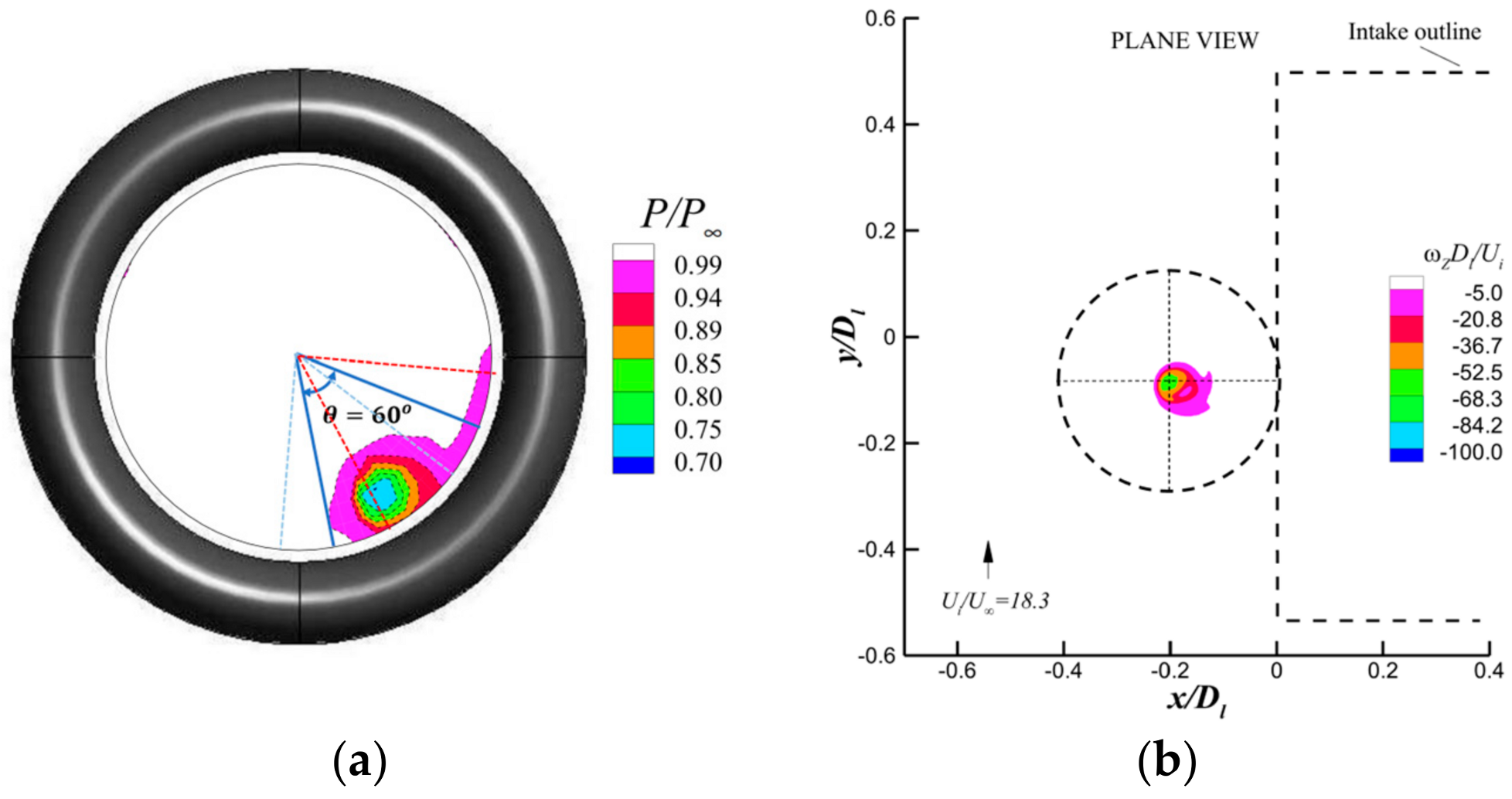
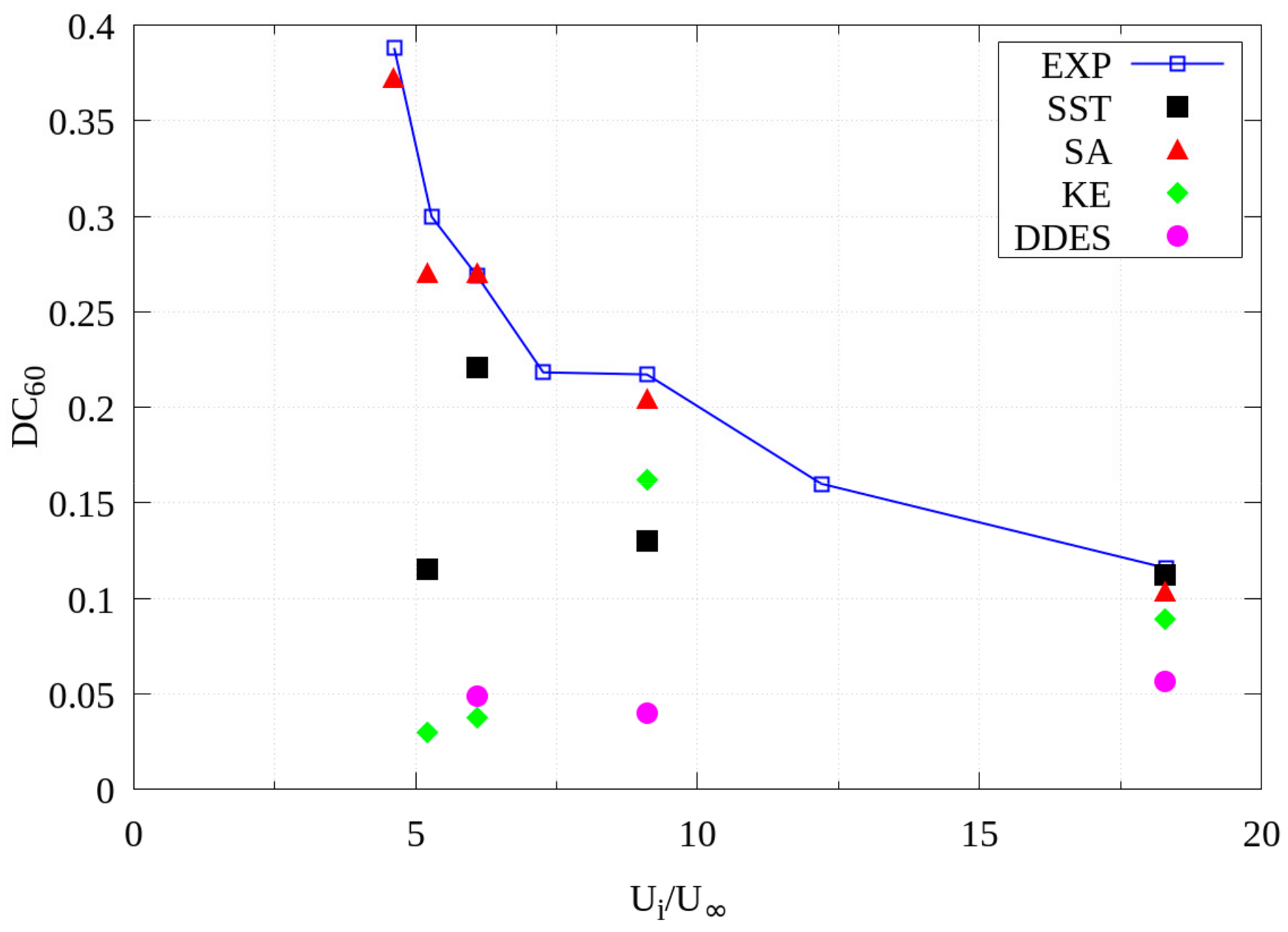
3.1. DC60

DC60 is a distortion index used to evaluate the total pressure loss ahead of the engine. It is defined as the difference between the area-averaged total pressure ${\overline{P}}_{t,AIP}$ and the area-averaged total pressure ${\overline{P}}_{t,60}$ within the worst 60-degree circumferential sector normalised by the average dynamic head ${\overline{P}}_f$ at the AIP, as shown in Figure 2a.

$$DC60={\displaystyle \frac{{\overline{P}}_{t,AIP}-{\overline{P}}_{t,60}}{{\overline{P}}_f}}$$

The quest of the worst 60-degree circumferential sector is implemented by trial and error, as indicated by the dashed line in Figure 2a. This sector has to cover the vortex core, though the largest total pressure loss can occur away from the vortex core when the crosswind speed is stronger.

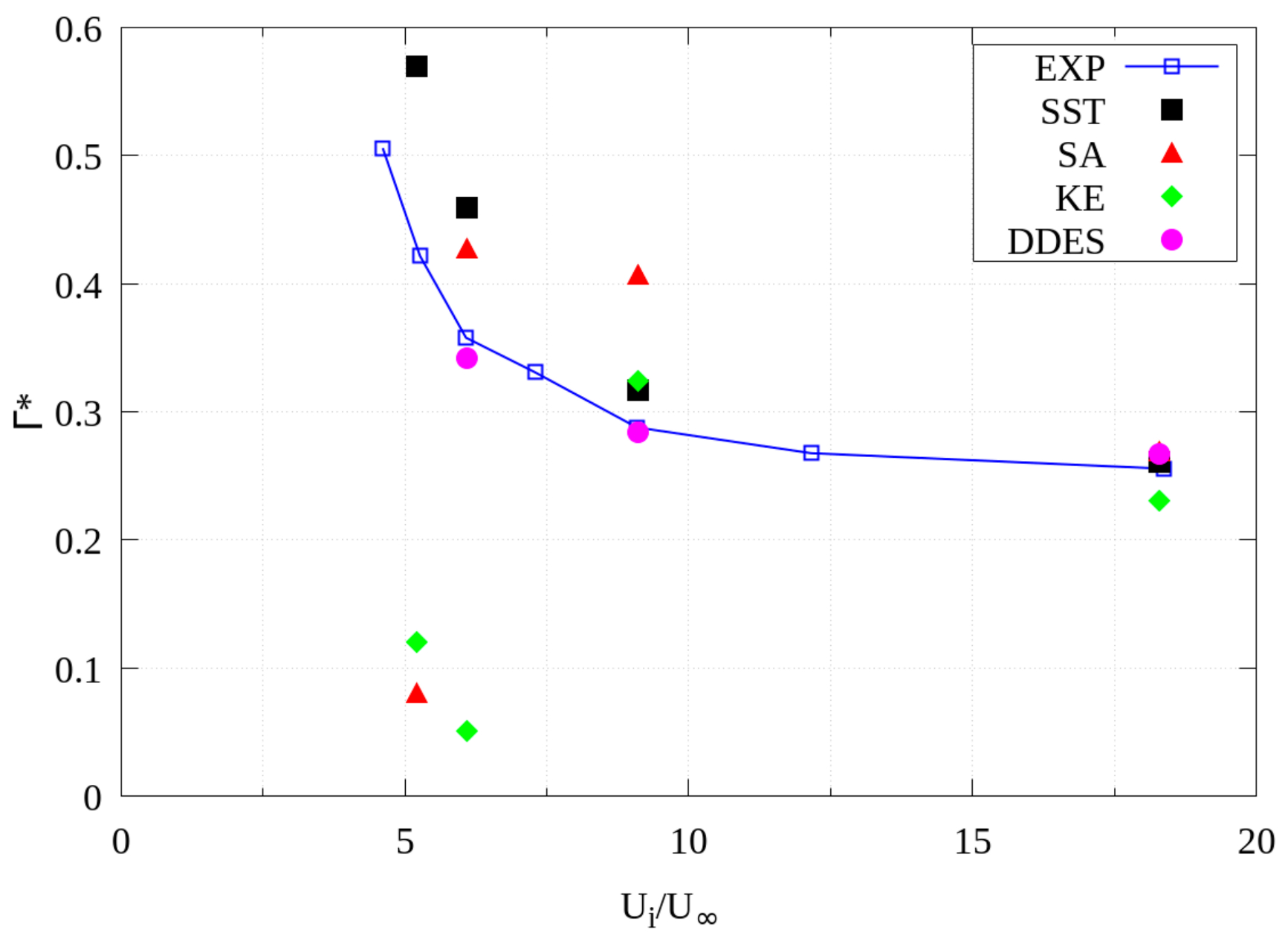
3.2. Circulation

To calculate the circulation of the ground vortex at the PIV measurement surface, a circle centred at the minimum point of the ${\omega }_z$ with a radius of 0.025 m is used to integrate the vorticity, as shown in Figure 2b.

$$\Gamma =\int {\omega }_{z}d{A}_c$$

where $A_c$ is the area of the circle. Since the vorticity is negative within the vortex core, only the negative value of ${\omega }_z$ is integrated. The total average non-dimensional vortex strength ${\Gamma }^{\ast }$ is obtained by dividing $\Gamma$ with the intake velocity $U_i$ and the diameter of the intake $D_l$. Further details about the computational procedure can be found in [10].

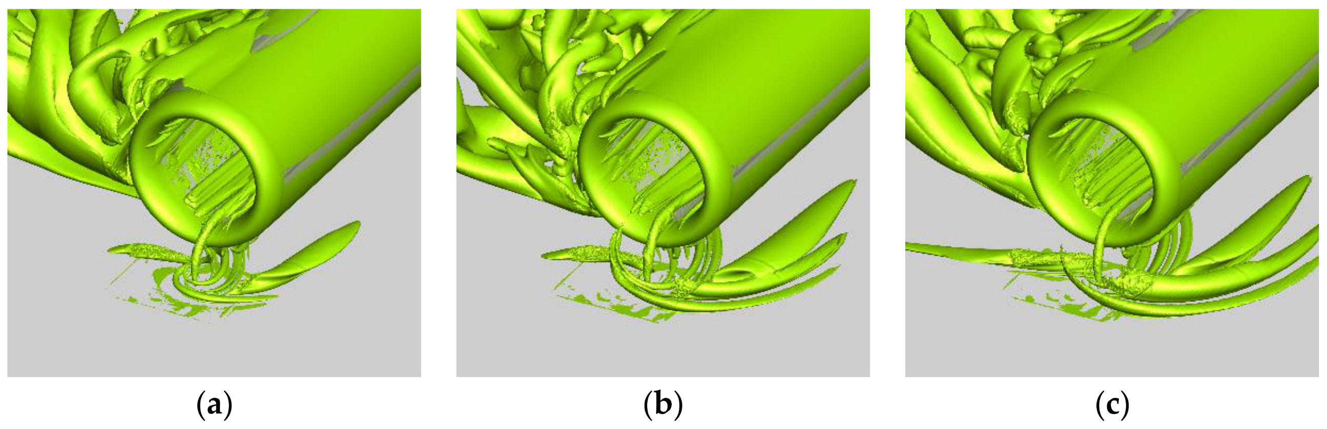
3.3. Q-Criterion

The value of Q of the flow field is computed using the following formula [28]:

$$Q={\displaystyle \frac{1}{2}}({\left|\mathsf{\Omega }\right|}^2+{\left|\mathrm{S}\right|}^2)$$

where $\mathsf{\Omega }$ and $S$ are the anti-symmetric and symmetric components of the velocity gradient tensor. In this work, the iso-surface of Q = 20,000 is used to identify the outline of the ground vortex unless otherwise stated. Figure 3 shows the contour of the ground vortex with the k—ω SST turbulence model for the velocity ratio $U_i/U_{\mathrm{\infty }}=18.3$. The trailing vortex at the leeward side of the intake and a ground vortex can be distinguished. The rotational direction of the vortex is clockwise when looking from top. The diameter of the ground vortex becomes larger when it is ingested from the ground surface into the intake.

4. Case Validation

4.1. Mesh Resolution

4.1.1. Mesh A

In this section, the simulated results with Mesh A are plotted against the experimental data to evaluate the performance of the CFD. Figure 4 displays the computed and measured normalised total pressure contours at the AIP for different crosswind speeds. These plots illustrate that the position of the vortex core at the AIP is at a more upwind position relative to the intake centreline due to the vortex–intake interaction. In the experiments, the vortex is pushed downwards as the crosswind speed becomes stronger. The total pressure loss caused by the ground vortex is also larger in terms of the range and amplitude. For the velocity ratio of $U_i/U_{\infty }=9.1$, the total pressure loss is trivial on the windward side of the intake while significant flow separation occurs at the condition $U_i/U_{\infty }=6.1$. The flow separation becomes more severe at higher crosswind speed. Affected by the ground vortex, the flow separation near the intake lip does not sit near the circumferential position $\theta =90$ but shifts along the anti-clockwise direction.

For the velocity ratio from 18.3 to 6.1, the computed pattern of the total pressure is very similar to those in the experiments. The pre-cited circumferential and radial position of the vortex also agree well with the measured data. However, the CFD results substantially underpredict the total pressure loss caused by the ground vortex at the AIP for all four conditions. The flow separation near the intake lip is also less for $U_i/U_{\infty }=6.1$. The ground vortex in the CFD is even blown away when the velocity ratio increases to $U_i/U_{\infty }=5.2$. However, the total pressure loss near the windward lip is overpredicted. For this case, a possible reason is that the CFD fails to present the strong velocity gradient for the ground vortex. With the absent of the ground vortex, to reach the same mass flow, the separation region near the windward lip becomes larger to account for the mass flow loss caused by the vortex. Another interesting observation is that the shape of the vortex core is more oval than that in the experiments.

The simulated average vector field and the non-dimensional out-of-plane vorticity (${\omega }_z{D}_l/U_i$) for four different velocity ratios are compared against the experimental data in Figure 5. In the experiments, it can be seen that the foot of the vortex on the ground plane shifts downwind as the crosswind blows harder and the vorticity at the vortex core becomes larger. Though the diameter of the vortex at the AIP expands with increased crosswind speed (Figure 4), it is not sensitive to the crosswind strength near the ground plane. The distance along the X direction between the vortex core and the intake outline in the experiments gradually increases with the crosswind speed. This trend is also captured by the CFD. However, neither the position or the vorticity strength of the ground vortex is accurately reproduced. The computed vortex diameter slightly increases and the vorticity of the vortex core is basically unchanged.

4.1.2. Mesh B

A further inspection of the mesh indicates that the spatial resolution is insufficient to resolve the large velocity gradient within the ground vortex. The grid of the PIV measurement plane is shown in Figure 6a. To remedy this problem, Mesh B is generated based on a posteriori knowledge from the experimental results: the region where the vortex may appear for different crosswind speeds is specifically refined. Structured mesh is generated near the boundary layer, and unstructured mesh is used to fill the region in front of the intake highlight plane. The comparison of Mesh B at the PIV measurement plane with Mesh A is shown in Figure 6. The grid size of Mesh A in this region is 4 mm × 4 mm and 0.35 mm × 0.35 mm in Mesh B. The node number at the AIP surface in Mesh B is 5.5 times that of Mesh A. To keep the element number the same with Mesh A, the far-field region is further coarsened especially the mesh above the intake along the Z direction.

With Mesh B, the computations are carried out again with exactly the same numerical strategies (Figure 7). It can be seen that for the lowest crosswind case $U_i/U_{\infty }=18.3$, the match between the CFD and EXP is significantly improved than that with Mesh A. The size of the region with total pressure loss ($P/P_{\infty }<0.99$) can be used to depict the diameter of the ground vortex at the AIP. Compared with the results obtained with Mesh A, it can be seen that the ground vortex is slimmer with Mesh B. The total pressure of the vortex core is still higher than the measured data though the simulated result has already been ameliorated. The position of the vortex at the AIP is nearer to the centreline than the experimental data. The position of the ground vortex at the PIV measurement plane is accurately captured for the case of $U_i/U_{\infty }=18.3$. For velocity ratio of $U_i/U_{\infty }=9.1$ and $U_i/U_{\infty }=6.1$, the vortex gradually moves downwind but less than the measured results. However, for the velocity ratio of $U_i/U_{\infty }=5.2$, the foot of the vortex moves upwind and shifts to a location similar to that of $U_i/U_{\infty }=9.1$. The distance between the vortex core and the intake outline along the X direction is accurately represented for all crosswind speeds. The pressure loss near the windward lip is still underpredicted for $U_i/U_{\infty }=6.1$ and overpredicted for $U_i/U_{\infty }=5.2$. The out-of-plane vortex strength for the case of $U_i/U_{\infty }=18.1$ is satisfactory in the simulation. For higher crosswind cases, the vortex strength is still underpredicted though they have been improved. For the case $U_i/U_{\infty }=4.6,$ the vortex is pushed to the leeward lip of the intake (Figure 8). The strength of the total pressure loss at the AIP as well as the non-dimensional out-of-plane vorticity has a large deviation from the measured data. No ground vortex is observed in the CFD with the $k-\omega$ SST model for higher crosswind speed.

Though it has been widely known that the mesh resolution is an important factor in order to enhance the numerical prediction capability, the mesh refinement seems to be invalid with high crosswind speed using $k-\omega$ SST turbulence model. In the following part, different turbulence models will be attempted.

It is worth mentioning that moving the downwind surface further downstream (extending the domain along Y direction) can improve the computed results to acquire better comparisons at a stronger crosswind speed [22]. This is not validated in the currently work; but, generally, a larger computational domain can reduce the influence of the downstream boundary condition on the concerned flow field.

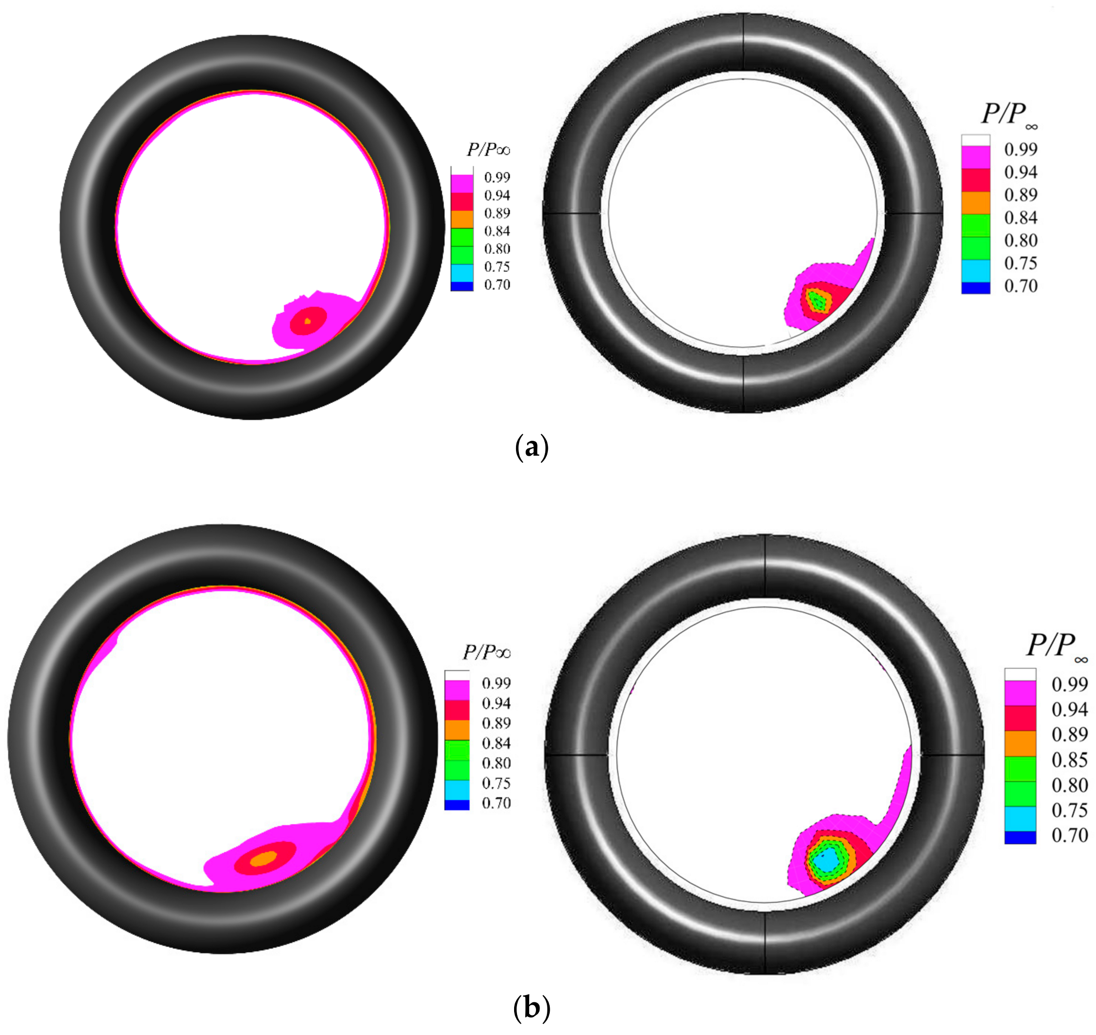
4.2. Turbulence Model

In this section, different turbulence models are tested. Firstly, the SA turbulence model is adopted with Mesh B and all other setup remains the same. The performance of the SA model is shown in Figure 9. The results with the SA turbulence model share some common features with the $k-\omega$ SST model: the predicted total pressure loss at the AIP surface is still less than the experimental data. The location of the vortex foot is almost the same as the $k-\omega$ SST model while the strength of the vorticity is obviously lower. For higher crosswind speeds from $U_i/U_{\infty }=5.2$, the vortex foot moves upwind and deviates from the measured scene. The separation-induced total pressure deficit is larger than the measured data. The results with SA model are less satisfactory than the $k-\omega$ SST model in terms of the total pressure and vorticity. The size of the vortex is also larger with the SA turbulence model. However, a noteworthy advantage of the SA turbulence model is its capability to maintain the ground vortex with very high crosswind speed. The vorticity at the PIV measurement plane generally remains the same with the increase in the crosswind speed. The position of the vortex core at the AIP surface is further from the centreline than the measured results. When the crosswind increases further to $U_i/U_{\infty }=4.0$, the ground vortex is finally blown away, as shown in Figure 9f. This prediction agrees well with the empirical value in the vortex formation map (vortex is not formed when $U_i/U_{\infty }<4.4 at{\displaystyle \frac{h}{Dl}}=0.25$) [7,14].

In fact, for the large crosswind speed, the steady simulation cannot lead to a converged solution. The mass flow across the intake has a relatively large oscillation due to the interaction between the ground vortex and the lip separation. The position and the strength of the ground vortex become unsteady, which are strengthened with the increase in the crosswind. Such unsteadiness behaviour of the ground vortex has been discussed in [4,23].

Figure 10 shows the simulated result with the $k-\epsilon$ turbulence model. Its poor performance in the prediction of the total pressure can clearly be seen and the ground vortex is missing when the crosswind speed is larger than $U_i/U_{\infty }=6.1$.

In the DDES computations, the $k-\omega$ SST turbulence model is used for the RANS calculation. It is considered that the for the crosswind speed less than 30 m/s, $k-\omega$ SST can obtain better prediction results. The flow field for the DDES is time-averaged, and the results are shown in Figure 11. Limited by the computational resource, no simulation higher than $U_i/U_{\infty }=6.1$ is conducted. It can be seen that the peak total pressure loss in the vortex core at the AIP and the vorticity strength prediction have been improved by the DDES computation. The vorticity for $U_i/U_{\infty }=18.3$ is even higher than the experimental value in the core region. The radius of the vortex is generally unchanged at different crosswind speeds and it is smaller than the measured data. Another discrepancy from the measured results is that the position of the vortex at the AIP surface. It is driven to the leeward side for the case $U_i/U_{\infty }=6.1$.

To further validate and evaluate the performance of the different turbulence models, the total pressure predictions at the AIP for three different crosswind speeds are compared against the experimental data at a fixed radial position, which pass through the peak loss point in the core, as shown in Figure 12. This plot clearly demonstrates the circumferential position and the total pressure distribution of the vortex in both experiments and simulations. It can be seen again that for $U_i/U_{\infty }=18.3,$ DDES simulation can acquire better prediction results regarding to the peak total pressure loss and the circumferential position of the vortex. But, the circumferential range of the vortex with DDES is smaller than the experimental data. For the velocity ratio of $U_i/U_{\infty }=9.1$, the simulation with SA model can obtain better prediction of the vortex position while DDES still works better in the prediction of peak total pressure loss than the others. At the condition of $U_i/U_{\infty }=5.2$, the $k-\omega$ SST model outperforms the other turbulence models and exaggerates the lip flow separation due to the crosswind.

A summary of the DC60 and circulation for different crosswind speeds simulated with different turbulence models is plotted in Figure 13 and Figure 14, which can provide an intuitive picture of their performance. It is concluded that none of the models can accurately reproduce both parameters. It can be seen that the circulation computed with the DDES turbulence model matches better with the measurement data than the $k-\omega$ SST model. The SA turbulence model can obtain a fairly favourable distortion index even at the high crosswind speed. At the lower crosswind speed conditions, almost all turbulence models can obtain good prediction results. The challenge comes from the simulations with larger crosswind.

The configurations of the ground vortex with different turbulence models for $U_i/U_{\infty }=9.1$ are shown in Figure 15. The $k-\omega$ SST and DDES provide more flow details especially near the ground surface (e.g., the approaching boundary layer, the rotational direction of the vortex and the edge of the sucked streamtube) than the other two. The flow field with SA and $k-\epsilon$ seems to be more diffused and smeared. Again, the vortex diameter is more “slender” with $k-\omega$ SST and DDES, as displayed in Figure 7 and Figure 11.

Here, another validation of the CFD is presented regarding the circulation of the ground vortex. Experimental study has found that the circulation of the ground vortex equals to that of the trailing vortex. While the measurement of the circulation can be a cumbersome process, CFD provides a more convenient choice. Figure 16 shows the result of $U_i/U_{\infty }=18.3$ computed with $k-\omega$ SST model. Two rectangular slices are created. Slice A is set at Y = 0.08 m, and the Y component of the vorticity is integrated. Only the negative value is included as the vorticity of the trailing vortex is negative. The Z component of the vorticity on slice B is integrated, and only the negative vorticity is integrated. The ${\Gamma }^{\ast }$ of the ground vortex is −0.261, and the circulation of the trailing vortex is 0.264. It can be seen that the absolute value of the circulation for both vortices is almost the same. This verifies the findings in [7] and enhances the confidence that the simulations can accurately capture the physical phenomena at relative low crosswind speeds.

4.3. Inflow Turbulence Strength

The influence of the inflow turbulence strength is tested with the $k-\omega$ SST model for the condition of $U_i/U_{\infty }=18.3$. The normalised thickness of the boundary layer $\delta /D_l$ is 0.03 for all computations. The DC60 and ${\Gamma }^{\ast }$ for various turbulence strength are listed in

Table 2. DC60 and ${\Gamma }^{\ast }$ for various turbulence strengths.

Turbulence Strength	0.1%	1.0%	5.0%	10.0%
DC60	0.102	0.085	0.094	0.08
${\Gamma }^{\ast }$	0.296	0.292	0.284	0.289

. The results imply that ${\Gamma }^{\ast }$ remains unchanged with different turbulence strengths. However, the DC60 decreases with the increase in the turbulence strength.

4.4. Thickness of the Inflow Boundary Layer

As it is widely accepted that the startup of the ground vortex with crosswind is not directly related to the approaching vorticity, it is assumed that the strength of the ground vortex is insensitive to the inflow boundary layer thickness. Three different values of boundary layer thickness are tested in the DDES computations. The velocity profile at the upwind surface is plotted in Figure 17 where h means the height from the ground plane. The thickness of the boundary layer is denoted with $\delta /D_l=$ 0.12, 0.45 and 1.03.

The Q-criterion plot in Figure 18 clearly shows that the thickness of the approaching boundary layer is indicated by the vortex size just underneath the intake. As shown by the data in

Table 3. DC60 and ${\Gamma }^{\ast }$ for various boundary layer thicknesses.

$\mathbf{Boundary} \mathbf{Layer} \mathbf{Thickness} \mathit{\delta }/{\mathit{D}}_{\mathit{l}}$	0.12	0.45	1.03
DC60	0.0393	0.0407	0.0364
${\Gamma }^{\ast }$	0.268	0.281	0.270

, the DC60 at the AIP and circulation on the ground surface varies randomly when the thickness of the boundary layer varies, and basically the difference among them is very small. This finding agrees well with the observations in [8,10], and it further confirms that the strength of the ground vortex is irrelevant to the thickness of the approaching boundary layer. Nevertheless, the startup process of the ground vortex may be affected by the boundary layer.

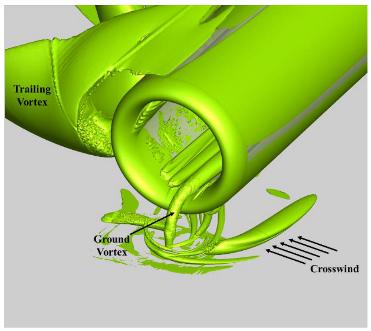
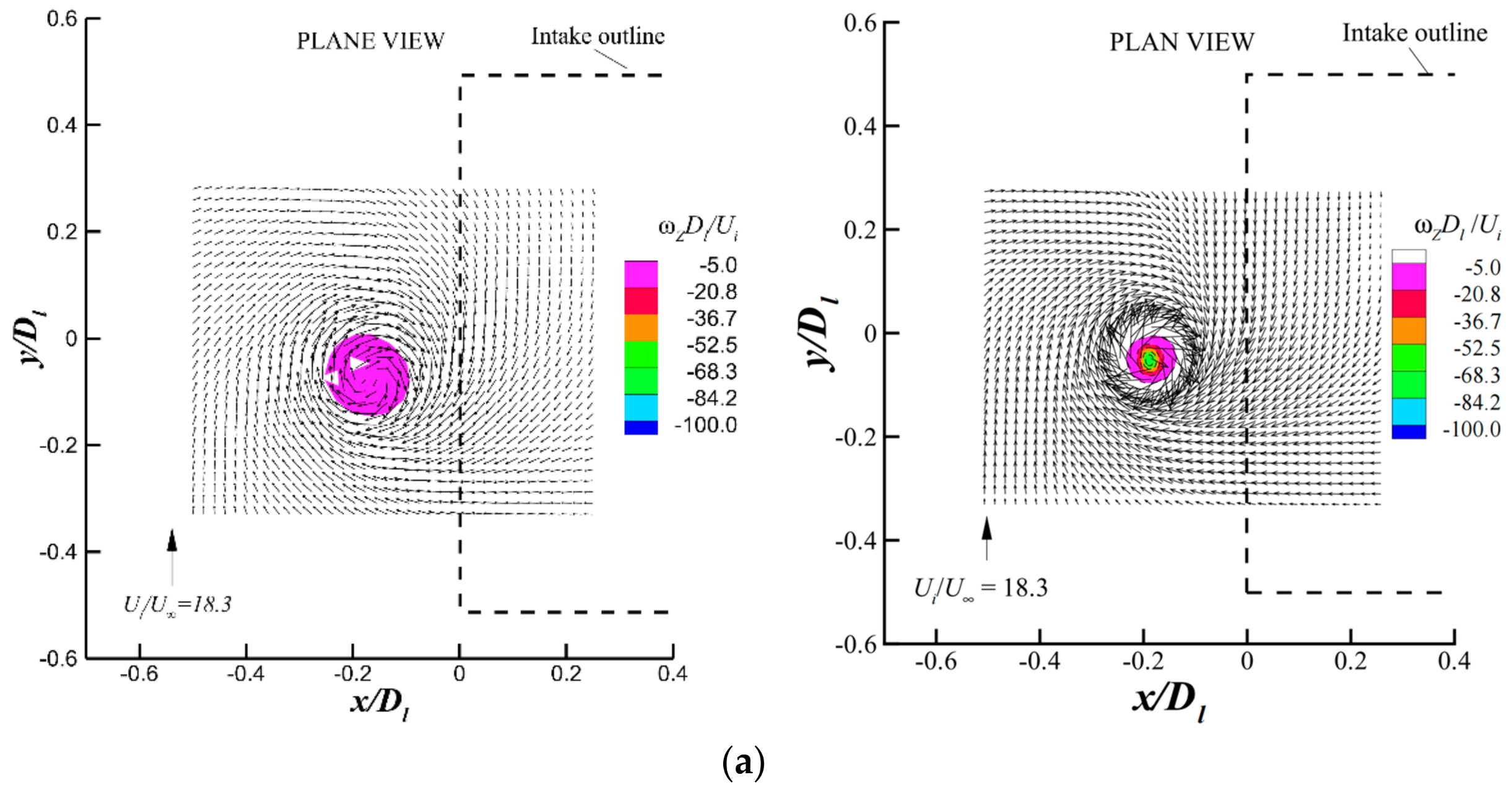
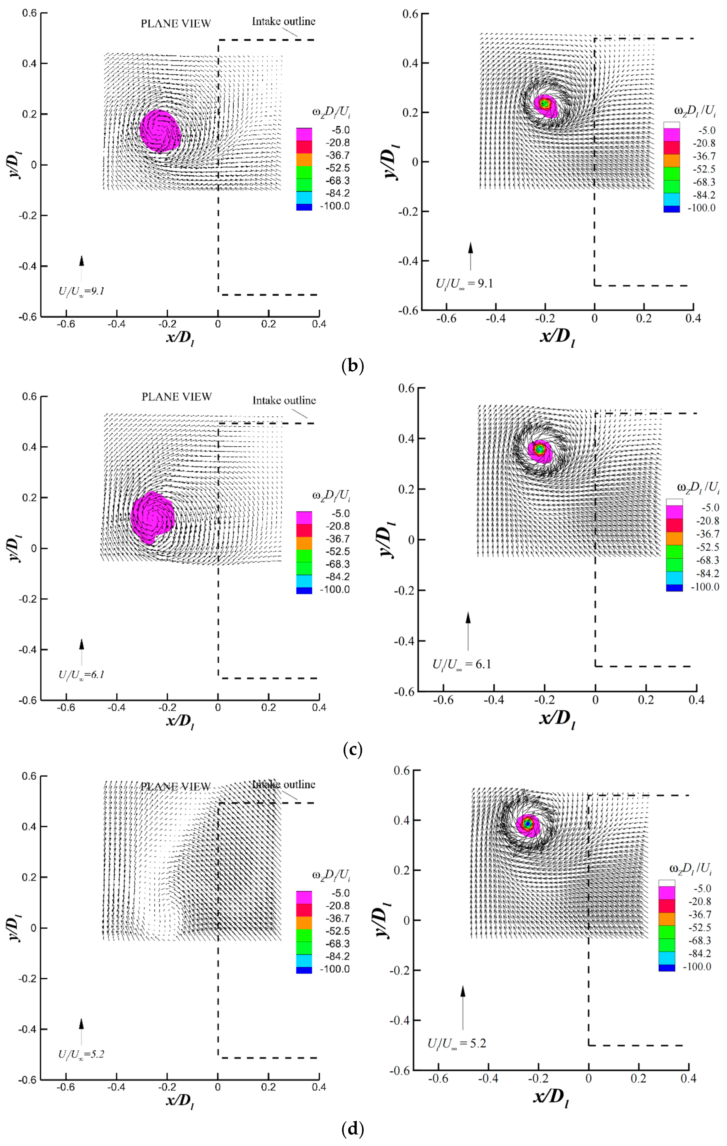
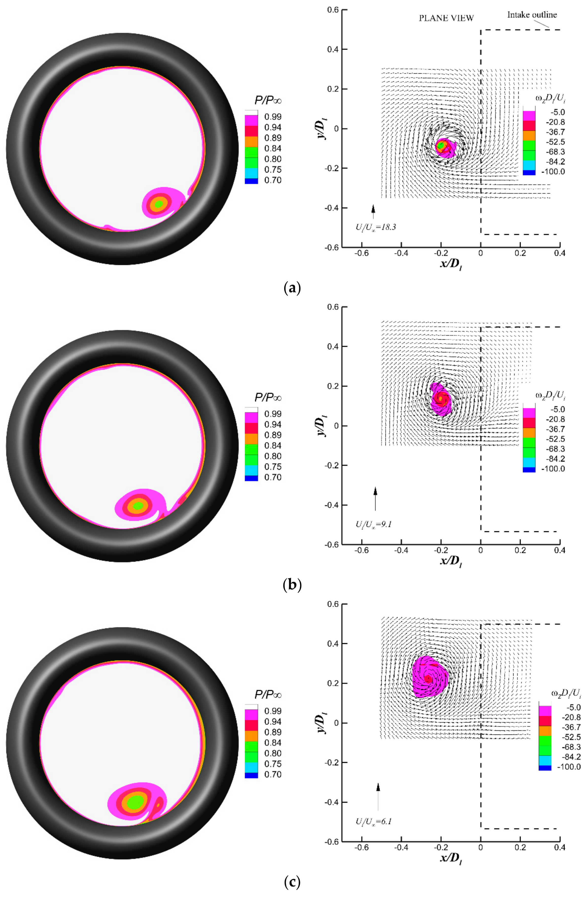
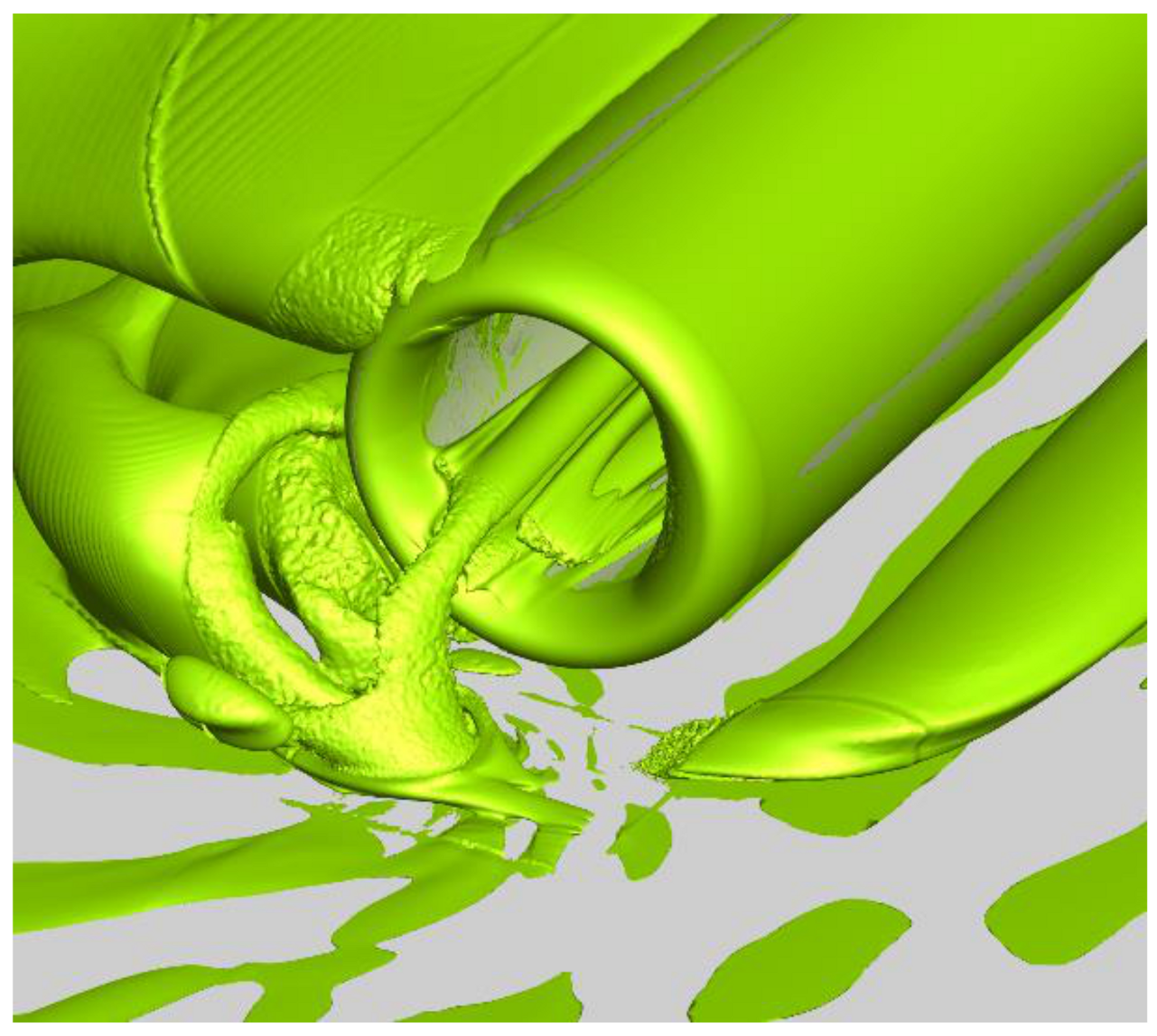
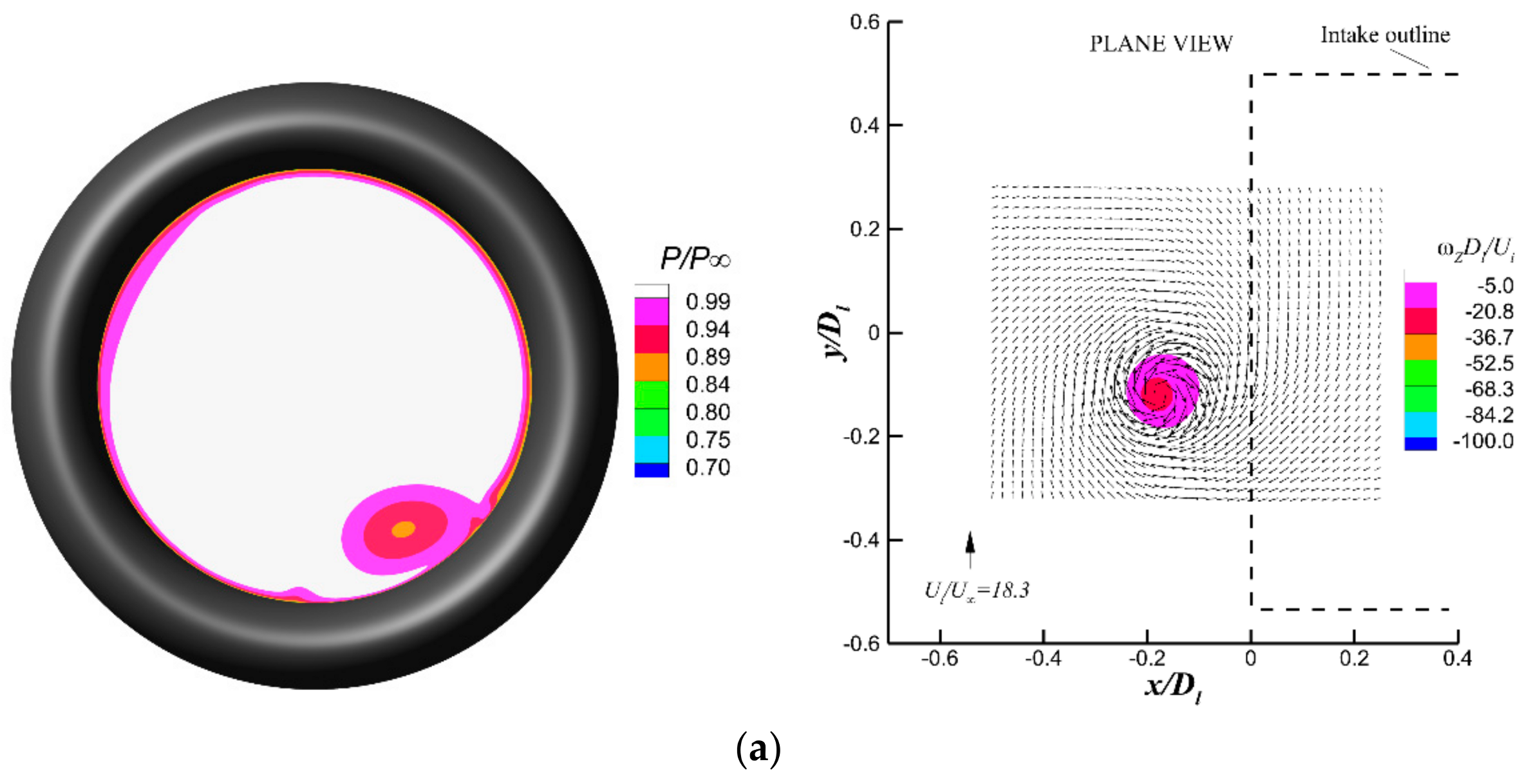
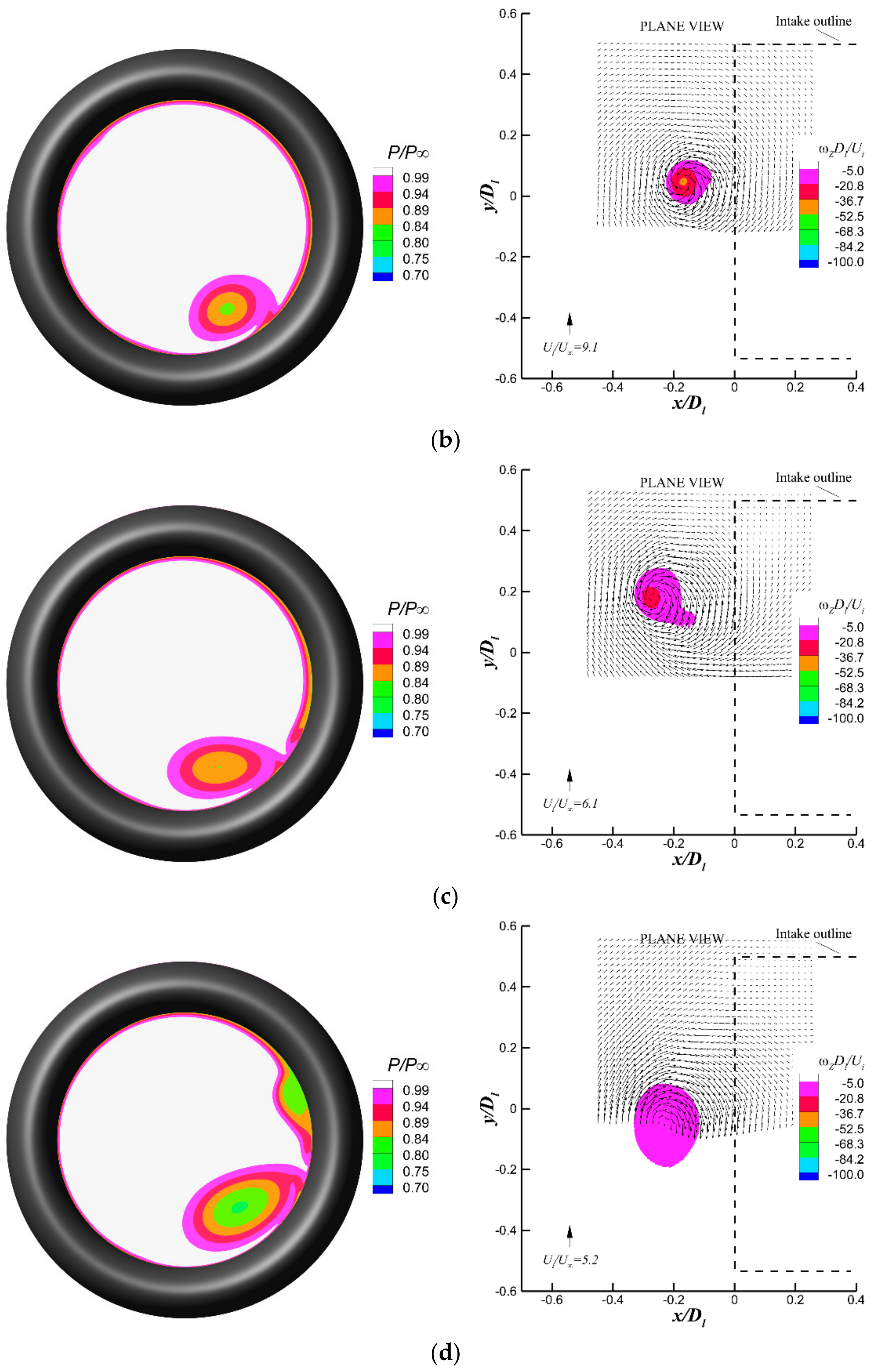
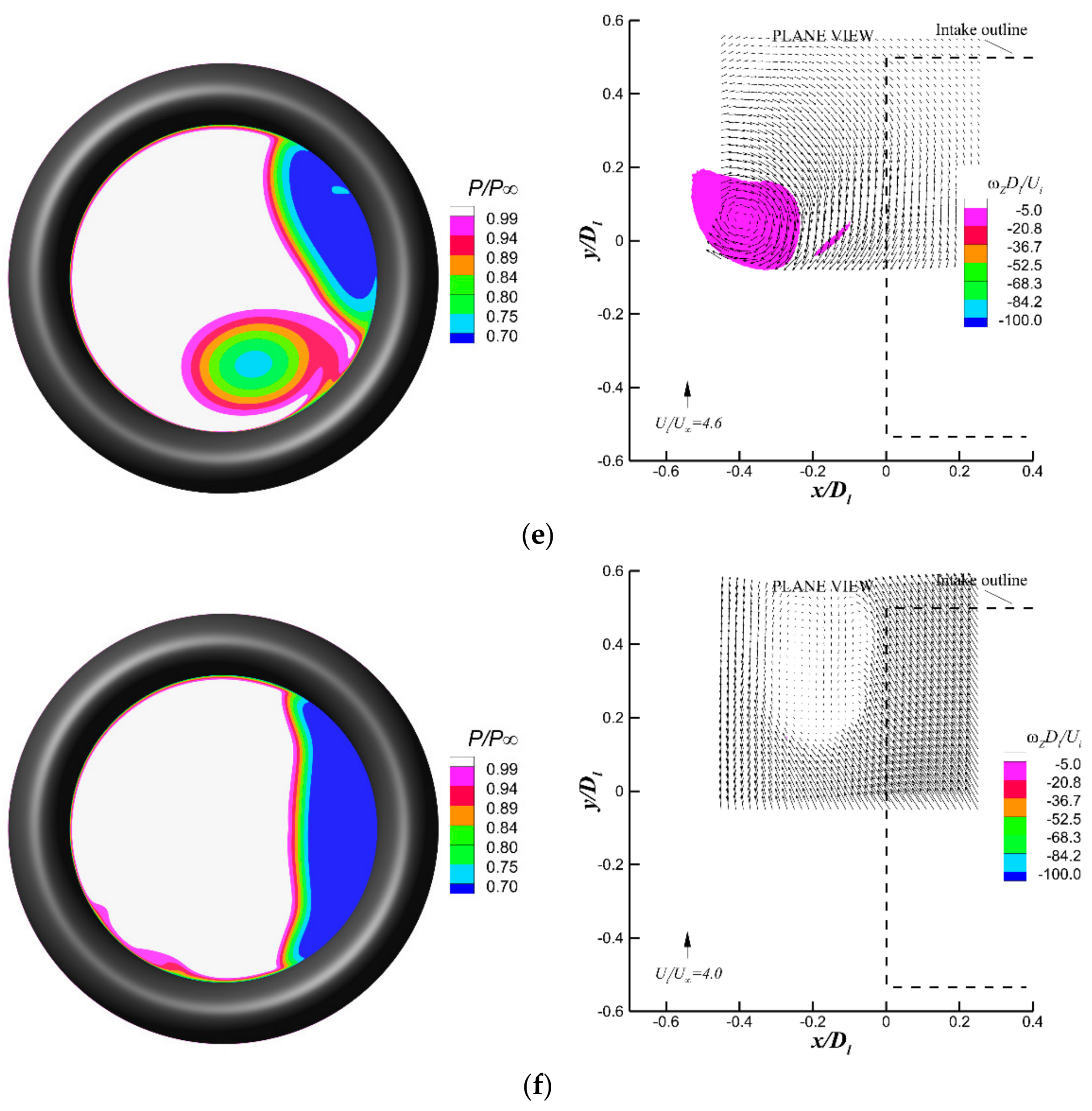
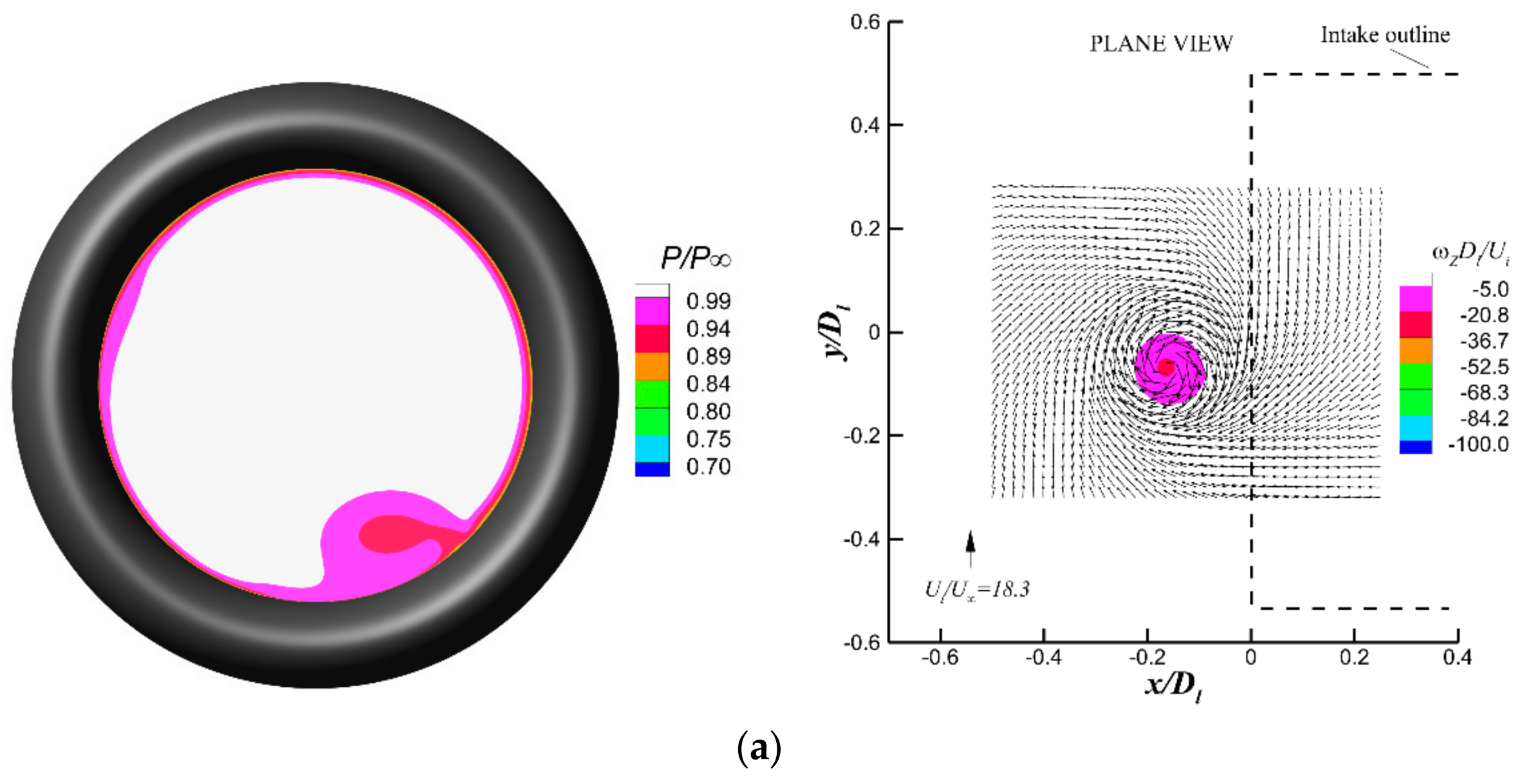
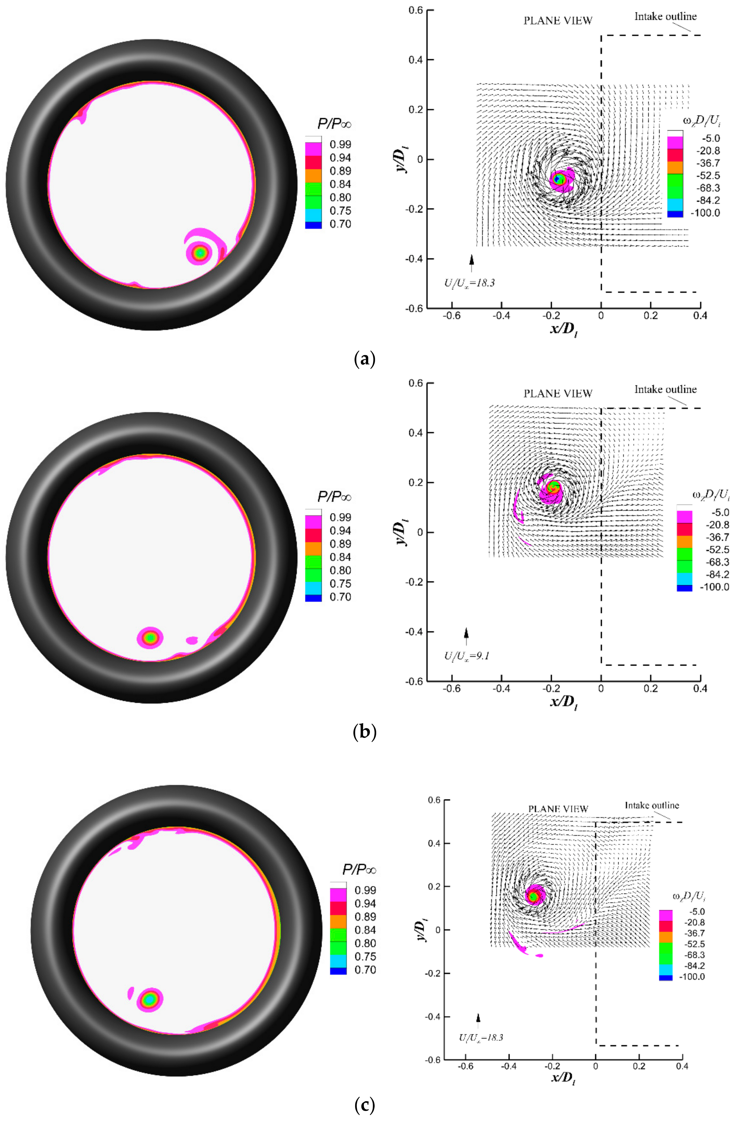
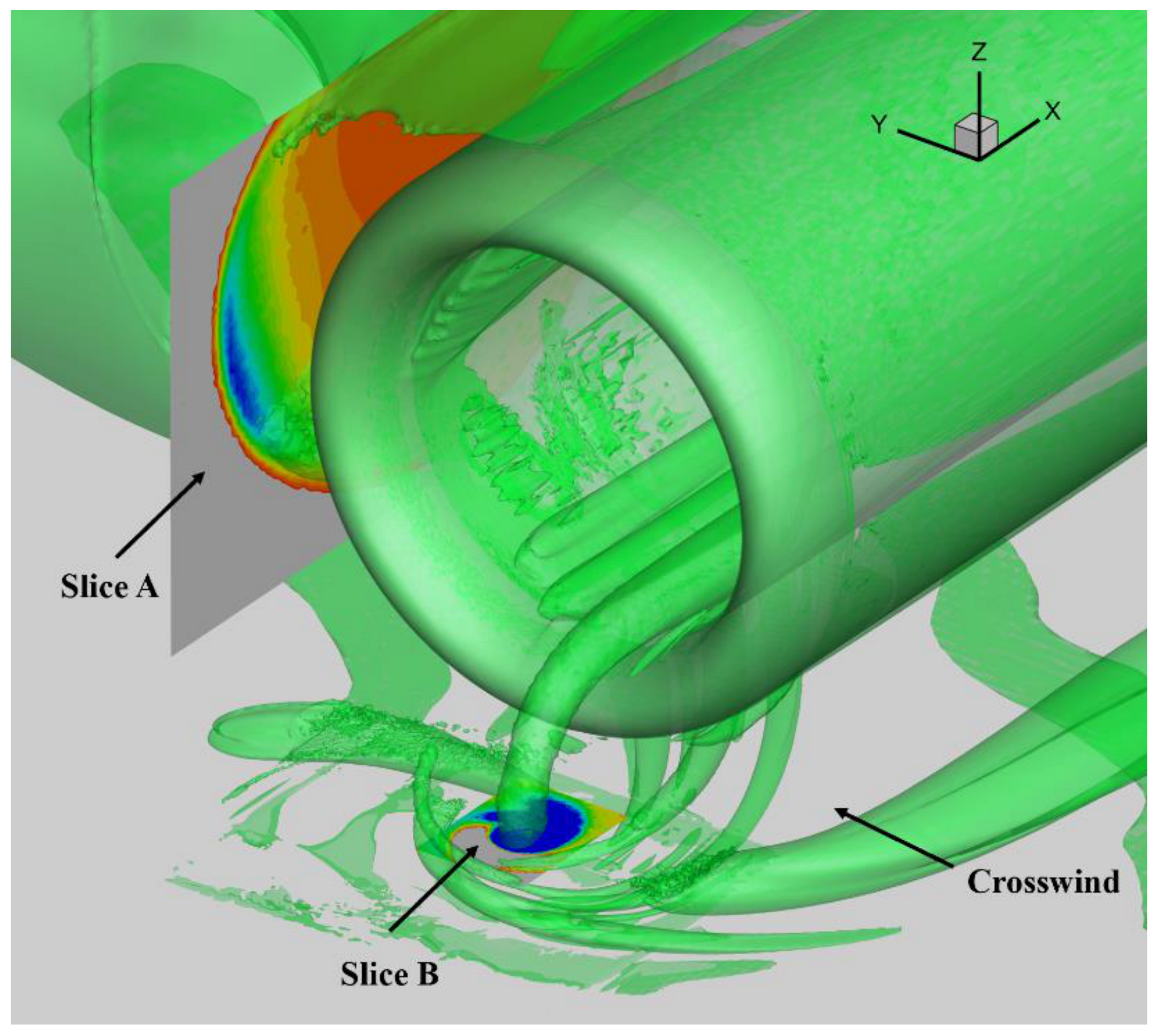
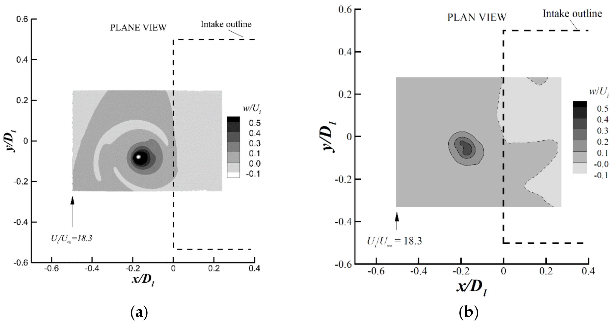
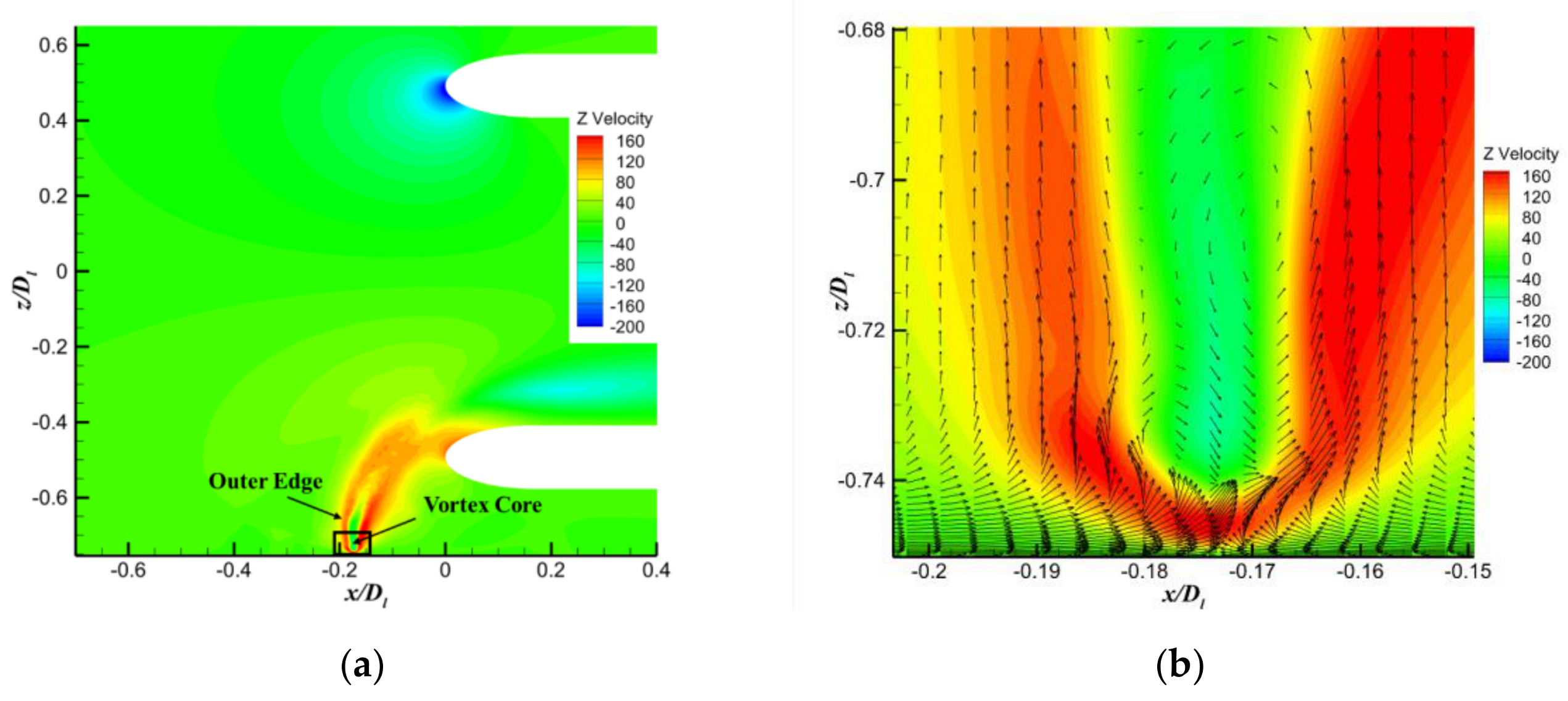
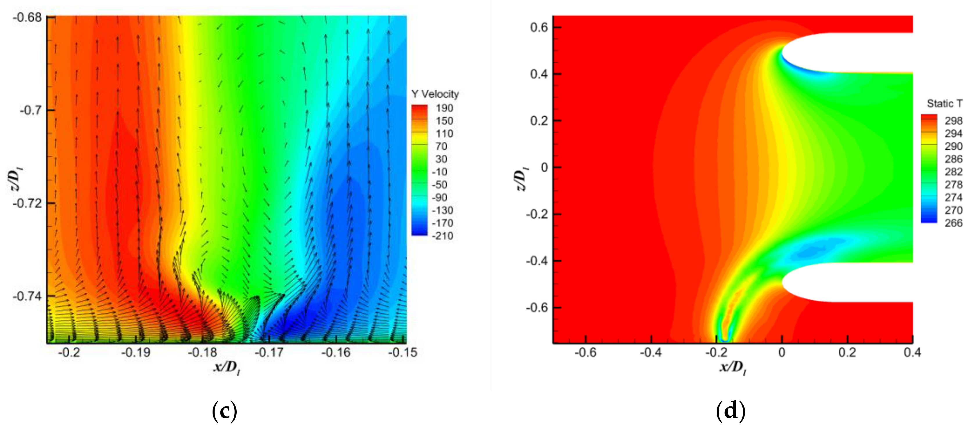
5. Flow Structure of the Ground Vortex

In this section, the structure of the ground vortex system with crosswind is further investigated. Figure 19a shows a zoomed view of the fully established vortex for the condition of $U_i/U_{\infty }=18.3$ with DDES simulation. The instantaneous streamlines into the intake are shown. The black streamlines denote the trace of the upper trailing vortex, which is formed when the shedding flow from the upper shell of the intake is ingested back into the tube. The blue ones represent the flow within the vortex core. The purple streamlines demonstrate the helical structure of the flow around the vortex core. The simulation captures the helical path of the streamlines around the vortex core observed in the experiments [29], as marked with the black arrow in Figure 19b. The red one denotes the lower trailing vortex, which starts from the lower shell of the intake. The yellow ones denote the flow sucked into the intake with no vorticity.

The surface streamline at the PIV measurement surface with the vortices is demonstrated in Figure 19c. The ground vortex is accompanied with the near-ground shear vortices, which are caused by the interactions between the suction flow into the intake and the main stream (i.e., the crosswind). The surface streamline on Slice A (Y = 0.025) in Figure 19b shows the reverse flow within the near-ground shear vortex. Another slice, Slice B cuts through the vortex core along the X direction, which will be discussed later. The lower tailing vortex has shifted its position and no longer hangs on the leeward side of the intake. In the flow field with a mature ground vortex, another near-ground shear vortex exists underneath the intake, which marks the boundary between the clockwise-rotating stream driven by the suction of the ground vortex and the main stream.

Figure 20 shows the simulated vertical velocity at the PIV measurement plane against the optical measurements. The figure shows that a white hole exists in the vortex core centre where the vertical velocity is very small. The measured velocity contour, however, is quit uniform inside the vortex core. As has been mentioned, such a discrepancy may come from the low-PIV resolution, which is not adequate to capture the inner flow pattern of the vortex core. Slice B in Figure 19b is generated to cut through the ground vortex. The vertical velocity on the slice is shown in Figure 21a. At the outer edge of the vortex, the vertical velocity is large as shown in the zoomed plot (Figure 21b). Such a flow pattern is just analogous to a tornado vortex [30,31,32], in which the vertical velocity is very low at the core region especially near the ground surface.

In the experimental study, it has been observed that most particles or pebbles [29,33] exposed on a flat ground surface will be moved away when the ground vortex passes by, and only a small portion will be lifted into the air. Even for the pebbles projected into the air by the vortex, they did not follow the path of the vortex core. Such a phenomenon can be explained with the flow structure shown in Figure 21b in this study. At the core region, the weak vertical velocity can hardly raise the peddles into the air; at the outer edge of the vortex, the vertical velocity increases, but the tangential velocity (i.e., Y velocity, Figure 21c) is even stronger, which generates a centrifugal force on the peddles and pushes the peddles out. The accurate prediction of the flow field with ground vortex is indispensable for the prediction of the movement of the foreign object inhalation. Figure 21d shows the temperature contour for the vertical slice. Significant flow acceleration happens above the lower lip of the intake with a large drop in the static temperature. In such a low temperature region, ice may be formed in the engine inlet when the vortex strength is sufficient to condense atmospheric moisture [29].

6. Discussions and Conclusions

In this paper, the numerical simulations of the ground vortex with crosswind are conducted and compared against the available experimental data. To tackle the challenge that the CFD fails to predict the flow field with the large crosswind speed, different numerical setups are tested to reduce discrepancies between the computations and experimental results. A recommended strategy to resolve the flow field with the ground vortex is to refine the mesh ahead of the intake, where the ground vortex exists. RANS computations are preferred for a time-averaged simulation. While DDES can obtain better prediction results at low crosswind speed, it consumes much longer CPU hours and is only suggested for the investigation of the basic flow mechanisms. Thereafter, the detailed flow structure of the ground vortex is demonstrated, which offers explanations for the experimental observations. The principles and conclusions of this work are summarised as follows:

• Mesh density is important for the simulation to accurately capture the total pressure loss and vorticity of the ground vortex as well as its position from the ground to the AIP surface. It is found that the mesh refinement is more remarkable for the cases with lower crosswind speed. In addition, it is considered that high-order schemes can also improve the CFD results and obtain better matches with the experimental data.
• Three most commonly used turbulence models with RANS are tested to demonstrate their performance. The computations with $k-\omega$ SST model can provide more detailed flow structures than the other two; though, the predictions of the total pressure loss at the AIP and the circulation near the ground for all three models are almost the same. SA turbulence model can reproduce the ground vortex with large crosswind speed and accurately predict the DC60. If the lowest total pressure value at the AIP is of interest, DDES with $k-\omega$ SST turbulence model should be used. In addition, DDES can obtain better prediction results in terms of the ground vortex circulation.
• The thickness of the boundary layer has almost no influence on the strength of the ground vortex in the simulation, and this further confirms the observation in the experiments. The circulation of the ground vortex seems to be unrelated to the turbulence strength. However, the distortion index decreases with the increment of the turbulence strength.
• The circulation of the trailing vortex and the ground vortex is equal, which further validates the finding in the experiments.
• The flow field with ground vortex is analysed to show the complex vortex system. Near-ground vortices are formed due to the interactions among the intake, crosswind and the ground vortex. The slice through the ground vortex indicates that its structure is similar to a tornado, where the vertical speed is very weak within the vortex core. The centre temperature of the vortex core can flow a lot due to the air acceleration.

References

- Johns, C. The aircraft engine inlet vortex problem. In Proceedings of the AIAA’s Aircraft Technology, Integration, and Operations (ATIO) 2002 Technical Forum, Los Angeles, CA, USA, 1–3 October 2002. [Google Scholar]
- Motycka, D.L. Ground Vortex–Limit to Engine/Reverser Operation. J. Eng. Power 1976, 98, 258–263. [Google Scholar] [CrossRef]
- Liu, K.; Sun, Y.; Zhong, Y.; Zhang, H.; Zhang, K.; Yang, H. Numerical investigation on engine inlet distortion under crosswind for a commercial transport aircraft. In Proceeding of the 29th Congress of the International Council of the Aeronautical Sciences, St. Petersburg, Russia, 7–12 September 2014. [Google Scholar]
- Wang, Z.; Chen, Y.; Ouyang, H.; Wang, A. Investigation on the Dynamic Response of a Wide-Chord Fan Blade Under Ground Vortex Ingestion. Int. J. Aeronaut. Space Sci. 2019, 20, 405–414. [Google Scholar] [CrossRef]
- di Mare, L.; Simpson, G.; Sayma, A.I. Fan forced response due to ground vortex ingestion. In Turbo Expo: Power for Land, Sea, and Air; American Society of Mechanical Engineers: New York, NY, USA, 2006; Volume 42401. [Google Scholar]
- Bissinger, N.C.; Braun, G.W. On the Inlet Vortex System. No. NASA-CR-140182. 1974. Available online: https://ntrs.nasa.gov/citations/19740027081 (accessed on 26 July 2024).
- Shin, H.W.; Greitzer, E.M.; Cheng, W.K.; Tan, C.S.; Shippee, C.L. Circulation measurements and vortical structure in an inlet-vortex flow field. J. Fluid Mech. 1986, 162, 463–487. [Google Scholar] [CrossRef]
- De Siervi, F.; Viguier, H.C.; Greitzer, E.M.; Tan, C.S. Mechanisms of inlet-vortex formation. J. Fluid Mech. 1982, 124, 173–207. [Google Scholar] [CrossRef]
- Brix, S.; Neuwerth, G.; Jacob, D. The inlet-vortex system of jet engines operating near the ground. In Proceedings of the 18th Applied Aerodynamics Conference, Denver, CO, USA, 14–17 August 2000. [Google Scholar]
- Murphy, J. Intake Ground Vortex Aerodynamics. 2008. Available online: https://dspace.lib.cranfield.ac.uk/items/4c4fe0c5-2aea-4237-bf76-2d2f65205047 (accessed on 26 July 2024).
- Murphy, J.P.; MacManus, D.G. Ground vortex aerodynamics under crosswind conditions. Exp. Fluids 2011, 50, 109–124. [Google Scholar] [CrossRef]
- Murphy, J.P.; MacManus, D.G.; Sheaf, C.T. Experimental investigation of intake ground vortices during takeoff. AIAA J. 2010, 48, 688–701. [Google Scholar] [CrossRef]
- Nichols, D.A.; Vukasinovic, B.; Glezer, A.; Rafferty, B. Formation of a Nacelle Inlet Ground Vortex in Crosswind. In Proceedings of the AIAA SCITECH 2022 Forum, San Diego, CA, USA, 3–7 January 2022. [Google Scholar]
- Liu, W.; Greitzer, E.M.; Tan, C.S. Surface static pressures in an inlet vortex flow field. J. Eng. Gas Turbines Power 1985, 107, 387–393. [Google Scholar] [CrossRef]
- Shmilovich, A.; Yadlin, Y. Engine ground vortex control. In Proceedings of the 24th AIAA Applied Aerodynamics Conference, San Francisco, CA, USA, 5–8 June 2006. [Google Scholar]
- Chen, J.; Wu, Y.; Hua, O.; Wang, A. Research on the ground vortex and inlet flow field under the ground crosswind condition. Aerosp. Sci. Technol. 2021, 115, 106772. [Google Scholar] [CrossRef]
- Zantopp, S.; MacManus, D.; Murphy, J. Computational and experimental study of intake ground vortices. Aeronaut. J. 2010, 114, 769–784. [Google Scholar] [CrossRef]
- Yadlin, Y.; Shmilovich, A. Simulation of vortex flows for airplanes in ground operations. In Proceedings of the 44th AIAA Aerospace Sciences Meeting and Exhibit, Reno, NV, USA, 9–12 January 2006. [Google Scholar]
- Karlsson, A.; Fuchs, L. Time evolution of the vortex between an air inlet and the ground. In Proceedings of the 38th Aerospace Sciences Meeting and Exhibit, Reno, NV, USA, 10–13 January 2000. [Google Scholar]
- Sylvain, R.; Costa, R.M.E.; Dupuy, F.; Becerril, C. Capturing intake ground vortex periodic patterns with affordable CFD simulations. In Proceedings of the 56th 3AF International Conference on Applied Aerodynamics, Toulouse, France, 28–30 March 2022. [Google Scholar]
- Rao, A.N.; Sureshkumar, P.; Stapelfeldt, S.; Lad, B.; Lee, K.B.; Rico, R.P. Unsteady analysis of aeroengine intake distortion mechanisms: Vortex dynamics in crosswind conditions. J. Eng. Gas Turbines Power 2022, 144, 121005. [Google Scholar] [CrossRef]
- Babcock, D.A.; Tobaldini Neto, L.; Davis, Z.; Karman-Shoemake, K.; Woeber, C.; Bajimaya, R.; MacManus, D. Summary of the 5th Propulsion Aerodynamics Workshop: Inlet Cross-Flow Results. In Proceedings of the AIAA SCITECH 2022 Forum, San Diego, CA, USA, 3–7 January 2022. [Google Scholar]
- Piovesan, T.; Wenqiang, Z.; Vahdati, M.; Zachos, P.K. Investigations of the Unsteady Aerodynamic Characteristics for Intakes at Crosswind. In Turbo Expo: Power for Land, Sea, and Air; American Society of Mechanical Engineers: New York, NY, USA, 2022; Volume 86113. [Google Scholar]
- Costa, R.M.E.; Millot, G.; Raynal, S.; Bouchet, J.P.; Courtine, S. Unsteady simulation of intake ground vortex ingestion in real wind tunnel conditions. In Proceedings of the 55th 3AF International Conference, Virtual, 12–14 April 2021. [Google Scholar]
- Secareanu, A.; Moroianu, D.; Karlsson, A.; Fuchs, L. Experimental and numerical study of ground vortex interaction in an air-intake. In Proceedings of the 43rd AIAA Aerospace Sciences Meeting and Exhibit, Reno, NV, USA, 10–13 January 2005. [Google Scholar]
- Available online: https://paw.larc.nasa.gov/paw5-inlet-test-case/ (accessed on 12 July 2022).
- Fluent, A. Ansys Fluent Theory Guide; Ansys Inc.: Canonsburg, PA, USA, 2021; pp. 41–158. [Google Scholar]
- Joeong, J.H. On the identification of a vortex. J. Fluid Mech. 1995, 285, 69–94. [Google Scholar] [CrossRef]
- Rodert, L.A.; Garrett, F.B. Ingestion of Foreign Objects into Turbine Engines by Vortices. No. NACA-TN-3330. 1955. Available online: https://ntrs.nasa.gov/api/citations/19930084118/downloads/19930084118.pdf (accessed on 26 July 2024).
- Nolan, D.S.; Farrell, B.F. The structure and dynamics of tornado-like vortices. J. Atmos. Sci. 1999, 56, 2908–2936. [Google Scholar] [CrossRef]
- Nolan, D.S.; Dahl, N.A.; Bryan, G.H.; Rotunno, R. Tornado vortex structure, intensity, and surface wind gusts in large-eddy simulations with fully developed turbulence. J. Atmos. Sci. 2017, 74, 1573–1597. [Google Scholar] [CrossRef]
- Snow, J.T. A review of recent advances in tornado vortex dynamics. Rev. Geophys. 1982, 20, 953–964. [Google Scholar] [CrossRef]
- Glenny, D.E.; Pyestock, N.G.T.E. Ingestion of Debris into Intakes by Vortex Action. 1970. Available online: https://reports.aerade.cranfield.ac.uk/handle/1826.2/1127 (accessed on 26 July 2024).