A Peak-Finding Siamese Convolutional Neural Network (PF-SCNN) for Aero-Engine Hot Jet FT-IR Spectrum Classification

Abstract

Aiming at solving difficulties related to aero-engine classification and identification, two telemetry Fourier transform infrared spectrometers are utilized to measure the infrared spectra of six types of aero-engine hot jets, and create a spectral data set, which is divided into a training set (80%), a validation set (10%), and a prediction set (10%). A peak-finding Siamese convolutional neural network (PF-SCNN) is used to match and classify the spectral data. During the training stage, the Siamese convolutional neural network (SCNN) is designed to extract spectral features and calculate the distance similarity. In order to improve the efficiency of the SCNN, a peak-finding method is introduced to extract the spectral peaks, which are used to train the model instead of the original spectral data. During the prediction stage, the trained model is used to calculate the similarity between the prediction set and the combined set of the training set and validation set, and the label of the most similar training data in each prediction set is used as the prediction label. The performance measures of the classification results include accuracy, precision, recall, confusion matrix, and F1-score. The experimental results show that the PF-SCNN can achieve a high classification accuracy rate of 99% and can complete the task of classifying the infrared spectra of aero-engine hot jets.

1. Introduction

The categorization features of aero-engines are frequently connected to the fuel type, combustion mode, and emission characteristics. Varied types of aero-engines will create varied gas compositions and emissions during combustion. Specific infrared absorption and emission spectra are formed through the vibrations and rotations of these molecules. Infrared spectroscopy [1,2,3] is a technique employed for the purpose of detecting the molecular structure and chemical composition of substances. Infrared spectroscopy determines the wavelength and intensity of absorbed or emitted light by measuring the energy-level transitions of substance molecules under infrared radiation. It constructs a spectrum to analyze the molecular structure and determines the type and content of substances. The Fourier transform infrared spectrometer (FT-IR spectrometer) [4] provides a significant means for the measurement of an infrared spectrum. The interferometer is used to acquire an interferogram, while the interferogram is transformed into a spectrogram through the Fourier transform. The passive FT-IR spectrometer is frequently employed for the detection of air pollutants, offering omnidirectional data collection capabilities and enabling continuous, long-range, and real-time monitoring as well as rapid target analysis. This method is more appropriate for the measurement of the aero-engine’s hot jet spectrum.

When the aero-engine hot jet spectrum data set is established, the rapid classification of unknown spectrum data becomes the focus of our research. Current research primarily focuses on classifying hyperspectral images using spectral and spatial features, while the classification of higher resolution infrared spectra is in its early stages. This paper aims to investigate infrared spectrum classification. The hyperspectral image classification (HSIC) method provides us with the classification idea of the FT-IR spectra. The classical method of HSIC for spectrum classification is to extract spectrum features by dimensionality reduction methods such as PCA [5], ICA [6], and LDA [7]. The spectrum features are combined with SVM [8], XGBoost [9], Random Forests [10], neural networks [11] and other classifiers to complete the classification task [12]. Similarly, HSIC also uses deep learning methods for feature extraction, such as AE [13], RNN [14], CNN [15], Transformer [16], Siamese network [17], etc. A Siamese network is a specific network architecture utilized for assessing data similarity, which is achieved through the implementation of weight sharing between two networks. It is often used in target tracking [18,19], change detection [20], image registration [21], and other fields. There are three structures of the Siamese network [22], including the Siamese network in which two branches share weights, pseudo- Siamese networks in which two branches have independent weights, and two-channel networks in which two inputs are superimposed. Huang [23] uses the two-branch Siamese network to perform feature extraction and calculate feature similarity on the metric layer. JIA [17] and Miao [24] combine AE with the Siamese network, and Nanni [25] uses K-means clustering to extract barycenter input to the Siamese network and combine SVM to complete the classification. Liu [26] used a Siamese convolutional neural network (SCNN) to extract features and combined it with SVM to complete the classification. The FT-IR spectroscopic method employed in this paper diverges from conventional hyperspectral technology. Hyperspectral technology utilizes the dispersive spectrometer to collect the continuous narrow-band spectrum, generally measuring the band from visible light to the near-infrared region, while the FT-IR spectrometer collects the complete interferogram of the infrared region and converts it into the spectrum without imaging. Using a FT-IR spectrometer allows for the acquisition of detailed molecular-level spectral features, which provide the infrared characteristics of molecules and aid in their classification. Given the unique characteristics of FT-IR spectra, we have applied the spectral classification method from the HSIC [27,28] to develop a classification network for FT-IR spectra. The Siamese network [29,30,31] enables efficient feature extraction and simultaneous support without requiring an extensive amount of labeled data, making it the preferred approach in this study.

The SCNN is employed to perform spectrum matching similarity for the purpose of training and validating the data set. In the prediction process, predicted data are combined with the trained data, and a trained network is used to determine the similarity of data pairs. Subsequently, the labels of the prediction set are determined by associating them with the training set labels that exhibit maximum similarity, thereby completing the prediction process. To enhance the operational efficiency of the SCNN, a peak-finding (PF) method is introduced for spectrum peak extraction through peak-finding and counting high-frequency peak positions. The extracted peak data are then utilized instead of the original data for both training and prediction. Following the evaluation of the experimental results, the PF-SCNN designed in this paper achieves an accuracy rate of 99%, indicating promising prospects for application in spectrum classification and recognition.

The paper’s contributions can be summarized in three aspects:

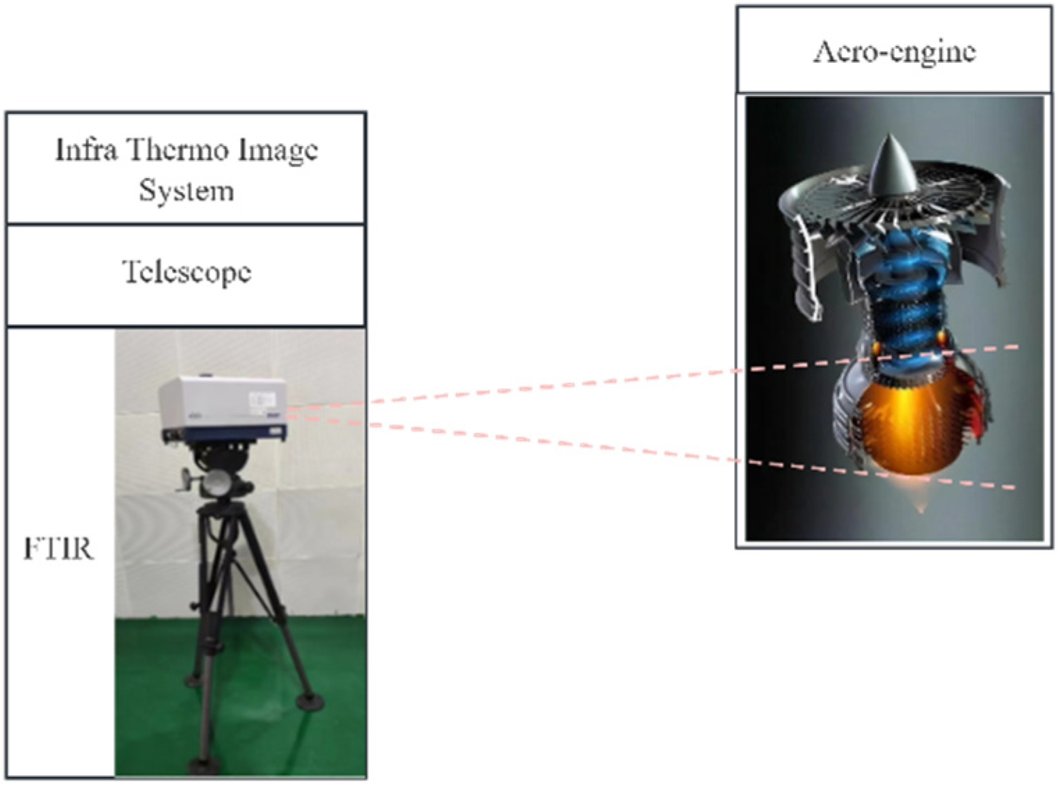
• To achieve the classification of aero-engines, this paper employs an infrared spectroscopy detection method to measure the spectra of aero-engines’ hot jets, which are significant sources of aero-engines’ infrared radiation, using an FT-IR spectrometer. The infrared spectra measured using the FT-IR spectrometer offers characteristic molecular-level information about substances, thereby enhancing the scientific basis for classifying aero-engines based on their infrared spectra.
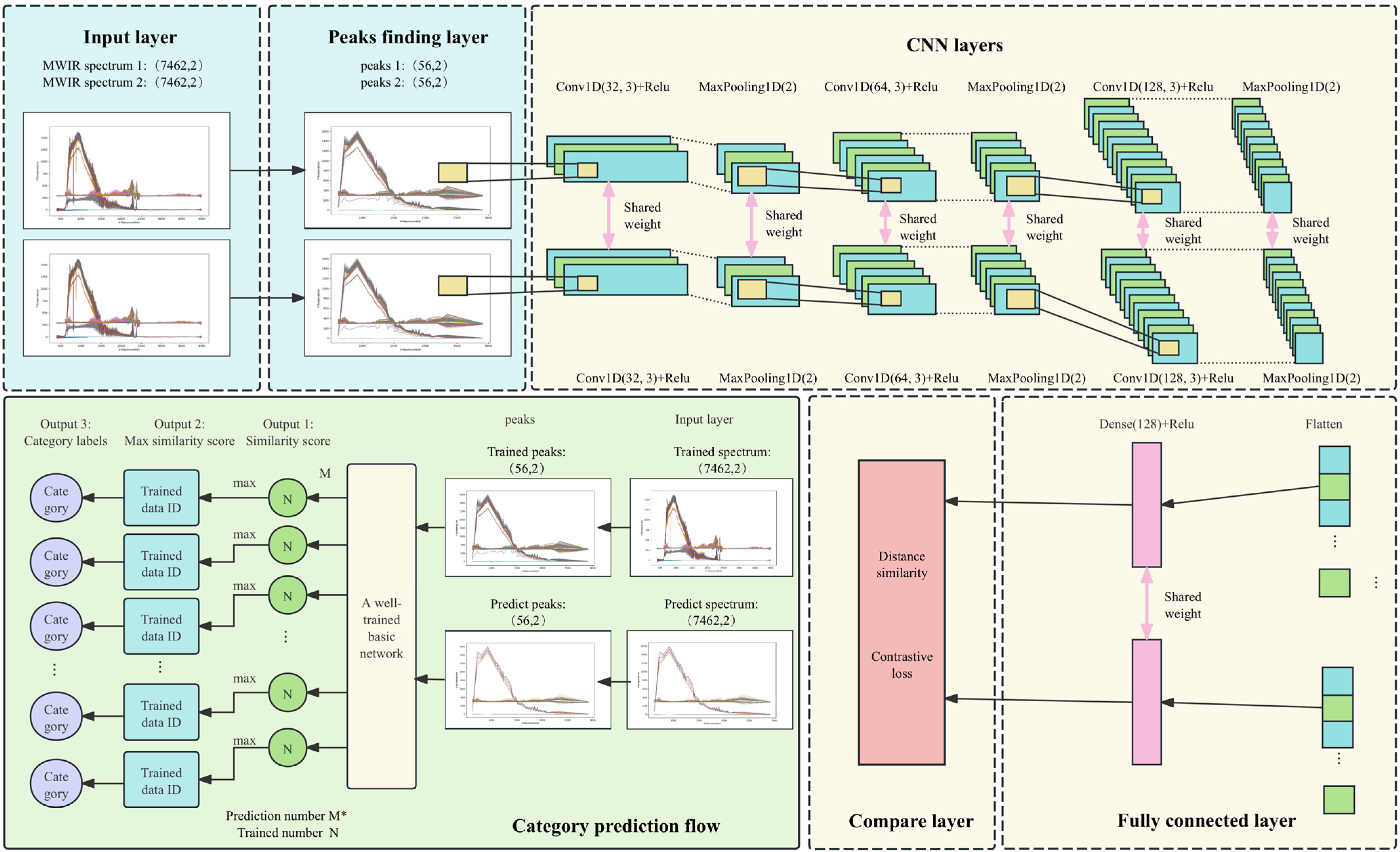
• This paper presents a SCNN for classifying the hot jet spectra of aero-engines using a data matching method. The network is based on 1DCNN, and feature similarity is calculated using the Euclidean distance metric. Subsequently, a spectral comparison method is employed for the purpose of performing spectrum classification.
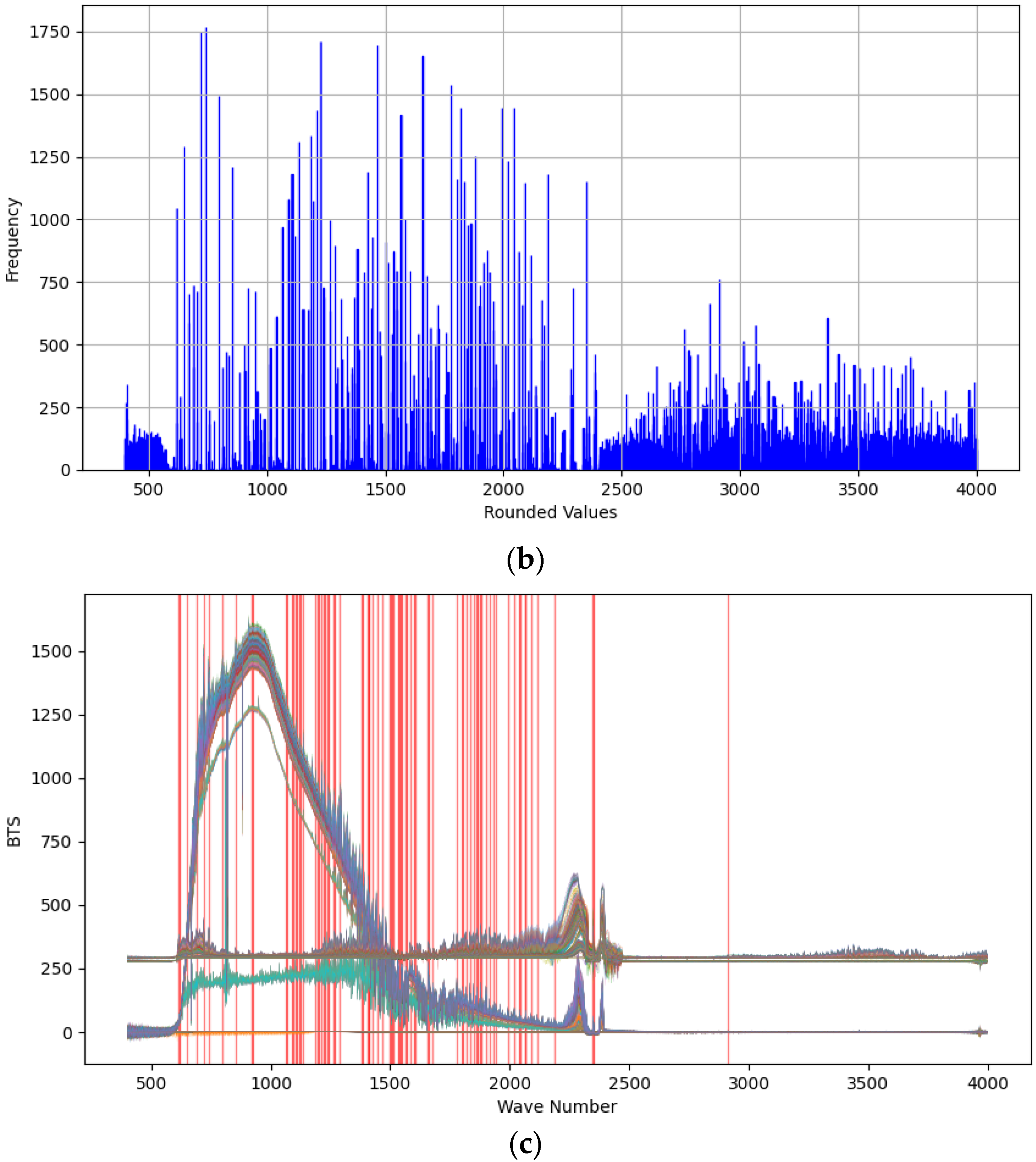
• The objective of this paper is to propose an algorithm for identifying peaks that will optimize the training and prediction speed of the SCNN. The algorithm identifies the peak value in the mid-infrared spectrum data and quantifies the high-frequency peaks, which are subsequently employed as input for the SCNN.

The paper is divided into five sections: Section 1 provides the research background, summarizes the current status of spectrum classification methods and Siamese networks, and briefly outlines the method, contributions, and structure of the paper. In Section 2, detailed descriptions are provided for the experiment on the aero-engine hot jet spectrum measurement design, data preprocessing, and spectrum data set production. Section 3 covers the PF-SCNN, encompassing the overall network design, base network design, peak-finding algorithm, and network training method. Section 4 analyzes the experiments and results, including performance measures and experiment outcomes, as well as the CO₂ feature vector classifier classification methods and ablation experiment analysis. Section 5 presents a summary of this paper.

2. Experimental Design and Data Set Production for Hot Jet Infrared Spectrum Measurement of Aero-Engines

The aero-engine hot jet infrared spectrogram measurement experiment and data set production are described in this section, which consists of the aero-engine spectrum measurement experiment design, spectrum data preprocessing, and data set production.

2.1. Aero-Engine Spectrum Measurement Experiment Design

Initially, we employed the outfield measurement method to gather infrared spectrum data of six types of aero-engine hot jets. The specific parameters of the two telemetry FT-IR spectrometers utilized in the experiment are detailed in

Table 1. Parameters of the FT-IR spectrometers used for the aero-engine hot jet measurement outfield experiment.

Name	Measurement Pattern	Spectral Resolution (cm−1)	Spectral Measurement Range (μm)	Full Field of View Angle
EM27	Active/Passive	Active: 0.5/1 Passive: 0.5/1/4	2.5~12	30 mrad (no telescope) (1.7°)
Telemetry Fourier Transform Infrared Spectrometer	Passive	1	2.5~12	1.5°

:

The experimental site layout is depicted in Figure 1:

The environmental parameters during the aero-engine hot jet measurement outfield experiment are presented in

Table 2. Environment parameters of the aero-engine hot jet measurement outfield experiment.

Aero-Engine Serial Number	Environmental Temperature	Environmental Humidity	Detection Distance
Engine 1 (Turbofan)	19 °C	58.5% Rh	5 m
Engine 2 (Turbofan)	16 °C	67% Rh	5 m
Engine 3 (Turbojet)	14 °C	40% Rh	5 m
Engine 4 (Turbojet UAV)	30 °C	43.5% Rh	11.8 m
Engine 5 (Turbojet UAV with propeller at tail)	20 °C	71.5% Rh	5 m
Engine 5 (Turbojet)	19 °C	73.5% Rh	10 m

:

The primary constituent of an aero-engine’s hot jet is the mixed gas, and its spectrum is contingent upon both the radiation emitted by the mixed gas itself and the combined influence of numerous intricate factors including pressure, temperature, humidity, and measurement distance. The performance of experiments affected by environmental factors is reflected in the following aspects: environmental temperature affects the spectrometer’s response, while environmental humidity influences the spectrum intensity. Additionally, the observed distance reflects the absorption and attenuation of the spectrum due to atmospheric transport along the measurement path.

At present, the experimental distance is relatively close, and the temperature of the mixed gas is also 300–400 °C, which is very different from the background temperature; so, the atmospheric and environmental impact can be temporarily ignored.

2.2. Spectrum Data Preprocessing and Data Set Production

The Brightness Temperature Spectrum [32] (BTS) is a widely used technology in passive FT-IR gas detection. The Brightness Temperature [K] of the actual object is equivalent to the temperature of the blackbody when the intensities of spectra are identical at the same wavelength.

The radiosity spectrum is equivalent to the BTS, which is represented by T(v), and can be obtained from the following formula:

$$T(v)={\displaystyle \frac{hcv}{k\ln \left\{\right[L(v)+2h{c}^2{v}^3]/L(v)\}}}$$

(1)

In the given expression, $v$ represents the wave number and the unit of wave number in cm⁻¹, while $L(v)$ pertains to the radiosity associated with wave number v. The $h=6.625\times {10}^{23} \mathrm{J}·\mathrm{S}$ denotes the Planck’s constant, $k=1.380649\times {10}^{-23} \mathrm{J}/\mathrm{K}$ stands for the Boltzmann constant, and $c=2.998\times {10}^8 \mathrm{m}/\mathrm{s}$ represents the speed of light.

The experimentally measured BTS after the conversion of the aero-engine hot jet is depicted in Figure 2, with the wave number on the horizontal axis and Kelvin temperature on the vertical axis. Additionally, key components of the hot jet are annotated in the figure.

The experimentally measured BTS after the conversion of the aero-engine hot jet is shown in Figure 2, where the horizontal coordinate is the wave number, and the vertical coordinate is the Kelvin temperature. Meanwhile, we have marked the important components of the hot jet in the figure.

Based on the outfield experiment and preprocessing, we acquire a spectrum data set, as illustrated in

Table 3. Data set of hot jet BTS from six types of aero-engines.

Number	Type	Number of Data Pieces	Number of Error Data	Full Band Data Volume	Mid-Infrared Range Data Volume
1	Engine 1 (Turbojet UAV)	193	0	16,384	7464
2	Engine 2 (Turbojet UAV with propeller at tail)	48	0	16,384	7464
3	Engine 3 (Turbojet)	202	3	16,384	7464
4	Engine 4 (Turbofan)	792	17	16,384	7464
5	Engine 5 (Turbofan)	258	2	16,384	7464
6	Engine 6 (Turbojet)	384	4	16,384	7464

:

There are 1851 valid spectrum data in the data set. In accordance with the principles of deep learning partitioning, we allocate the data into training, validation, and prediction sets at an 8:1:1 ratio. The training set includes 10,000 positive and 10,000 negative sample pairs selected randomly, while the validation set contains 1000 positive and 1000 negative sample pairs.

3. Architectural Design of Peak-Finding Siamese Convolutional Neural Network

In this section, the PF-SCNN is presented for classifying infrared spectra, comprising four key components: overall network structure design, base network architecture, peak-finding algorithm, and network training methodology.

3.1. Overall Network Structure Design

The Siamese network for data classification comprises three essential modules: feature extraction, sample comparison, and classification decision. The Siamese network diagram of this paper is depicted in Figure 3:

According to the SCNN module design above, the detailed PF-SCNN structure is designed as demonstrated in Figure 4. The PF-SCNN consists of three main parts: the peak-finding module, base network module, and classification prediction module.

During the training stage, positive and negative sample pairs are created with corresponding label sets. If the categories are the same, a label value of 1 is assigned; otherwise, a value of 0 is assigned. The mid-infrared spectrum peaks are extracted and detected in the peak-finding module. The input data and peak-finding module are shown in the blue background in the figure.

The base network layer is shown in the figure as the part with a yellow background color, consisting of the CNN layer, FC layer, and compare layer. It extracts features of data pairs, outputs distance similarity, and approximates the predicted labels of the training set to true labels through a comparison function, thus completing model training.

The classification prediction module is represented with a green background. At this stage, a data pair is established between the predicted data and all the trained data. The similarity score for each piece of predicted data in relation to all the trained data is computed by inputting it into the trained network. The maximum similarity score for each piece of predicted data is selected, and then the corresponding trained data number and category labels are utilized to finalize the prediction.

3.2. Base Network Architecture

The base network module is used to train the positive and negative sample pairs, complete the feature extraction of the above network, and compare the content of the two modules with the samples. The base network part consists of convolution layers, maximum pooling layers, a flattening layer, a fully connected layer, and a self-defined Lambda layer.

3.2.1. One-Dimensional Convolutional Layer (Cov1D Layer)

The convolutional layer extracts features, while the Cov1D layer performs linear and translation-invariant operations through convolution. This enhances signal characteristics and reduces noise.

The convolution between two functions, in terms of a mathematical expression, can be defined as $f,g:{\mathbb{R}}^d\to \mathbb{R}$:

$$(f\ast g)(\mathit{x})=\int f(\mathit{z})g(\mathit{x}-\mathit{z})d\mathit{z}$$

(2)

Convolution is the result of overlapping two functions, where one function is flipped and shifted by $\mathit{x}$. In the case of two-dimensional tensors, convolution can be represented as follows:

$$(f\ast g)(i,j)=\sum _a\sum _{b}f(a,b)g(i-a,j-b)$$

(3)

In the expression, $(a,b)$ is the index of $f$ and $(i-a,j-b)$ is the index of $g$.

3.2.2. Maximum Pooling Layer (MaxPool Layer)

The MaxPool layer, a component of the CNN, serves as a method for downsampling by reducing data processing while preserving essential information. Operations such as the convolution layer, pooling layer, and activation function layer can be interpreted as mapping original data to the feature space of hidden layers.

3.2.3. Flattening Layer

The flattening layer, positioned between the Cov1D and FC layers, converts the feature map from the former into one-dimensional feature vectors for input into the latter. This transformation is essential as it enables the fully connected layer to process one-dimensional input using the dot product of the weight matrix and input vector to compute output.

3.2.4. Fully Connected Layer (FC Layer)

The FC layer translates the learned distributed feature representation into the sample label space, combining and outputting them as a single value to reduce the impact of the feature position on the classifier.

3.2.5. Comparison Layer

Keras provides Lambda functions for creating a dedicated layer to apply function transformations to the data, in the form of a Lambda layer. Depending on our data comparison requirements, we can choose a distance function to compare two feature vectors. In data comparison, distance is commonly used as a constraint method for evaluating the similarity between two feature vectors. The distances of vectors typically include the Euclidean distance (L2 norm), Manhattan distance, Cosine similarity, Chebyshev distance, Hamming distance, Jaccard similarity, Pearson correlation coefficient, and others. We choose Euclidean distance, which can be expressed as follows:

$$(X_1,X_2)={\parallel X_1-X_2\parallel }_2={(\sum _{i=1}^P{(X_1^i-X_2^i)}^2)}^{{\displaystyle \frac{1}{2}}}$$

(4)

where $X_1$ and $X_2$ are two feature vectors. $P$ represents the number of feature vectors.

3.3. Peak-Finding Algorithm

The molecular structure of the substance has a direct influence on the intensity, frequency, and shape of the infrared spectrum, which is reflected in the number, position, shape, and intensity of the infrared spectrum. The important means of the infrared spectrum analysis involve analyzing the position, intensity, and shape of characteristic peaks; so, we construct a peak-finding algorithm to find the peaks [33].

The sliding window method is a commonly used method to find extreme values, which is mainly used to solve the problem of subsequences in arrays or linked lists. The basic idea is to find the desired extreme value by maintaining a window (that is, a continuous sequence of subsequences in an array or linked list) and dynamically adjusting the size and position of the window during sliding.

The formula for local maximum retrieval using the sliding window method is as follows:

$$x_i>x_{i-k},\dots ,x_{i-1} and{ x}_i>x_{i+1},\dots ,x_{i+k}$$

(5)

where $i$ is the current sequence number, $k$ represents the window threshold, and the window range is from $i-k$ to $i+k$.

The local minimum search formula is as follows:

$$x_i<x_{i-k},\dots ,x_{i-1} and x_i<x_{i+1},\dots ,x_{i+k}$$

(6)

The index of the local extremum $I_{max} and I_{min}$ can be found by using the following formula:

$$I_{max}=i\mid x_i>x_{i-1} and x_i>x_{i+1},1\le i\le n-2$$

(7)

$$I_{min}=i\mid x_i<x_{i-1} and x_i<x_{i+1},1\le i\le n-2$$

(8)

We use the peak-finding algorithm in the mid-infrared region and illustrate the operational flow of the algorithm using the following pseudo-code Algorithm 1:

Algorithm 1: Peak-Finding and Peak Statistics Algorithm

Input: Spectrum data

Output: Peak data

➀ Crop the mid-infrared band (400–4000 cm−1) of spectrum data. ➁ Execute data smoothing. ➂ Set the parameters of the sliding window peak-finding algorithm. ➃ Count the wavenumber position of each peak. ➄ Identify the wave number positions associated with high frequency by applying threshold value proportions. ➅ Extract the points near each data point as the peak data points according to the peak wave number position. ➆ Output peak data for each spectrum data.

3.4. Network Training Methodology

3.4.1. Optimizer

The optimizer method is a method for finding the optimal solution of a model. Commonly used optimizers include the gradient descent and the adaptive learning rate optimization algorithms. The former includes the standard gradient descent (GD), stochastic gradient descent (SGD), and batch gradient descent (BGD). The disadvantage of the GD method is the slow training speed and sensitivity to local optimal values. The latter includes the Adaptive Gradient (AdaGrad), Root Mean Square Propagation (RMSProp), Adaptive Moment Estimation (Adam), and Adaptive Delta (AdaDelta). Among them, the RMSProp optimizer with an adaptive learning rate adjustment has been chosen for this paper.

The RMSProp optimizer [34] is an optimization algorithm that adjusts the learning rate adaptively based on the moving average of the gradient square, providing different learning rates for each parameter and solving the problem of overly large or small learning rates in the SGD algorithm effectively. It uses the exponential decay average of historical gradients to adaptively adjust the learning rate.

The second-order momentum of the RMSProp V_t is calculated as follows:

$$V_t\leftarrow \beta \ast V_{t-1}+(1-\beta )g_t\odot g_t$$

(9)

where $t$ is a time step, $V_t$ is the second-order momentum of the current time step, and $V_{t-1}$ is the second-order momentum of the previous time step. $\beta$ is the decay rate of the historical second-order momentum, which is generally set to 0.9 and is used to control the decay rate of historical information, while $g_t$ is the gradient. $V_t$ pays more attention to the recent gradient and does not superimpose to infinity.

The learning rate of each element in the objective function argument is re-adjusted by the element operation, and then the formula of $w_t$ is updated as follows:

$$w_t\leftarrow w_{t-1}-{\displaystyle \frac{\eta }{\sqrt{V_t+ϵ}}}\odot g_t$$

(10)

where $\eta$ is the learning rate, $ϵ$ is a constant added to maintain numerical stability and the value is usually set to 10⁻⁶, and $\odot$ stands for the product of elements; the calculation method is $(A\odot B{)}_{ij}=(A{)}_{ij}(B{)}_{ij}$.

The RMSProp optimizer excels in handling large-scale non-convex optimization and deep learning problems by adaptively adjusting the learning rate to prevent it from vanishing. However, it suffers from hyperparameter dependence, as the choice of the attenuation factor and other parameters can significantly impact its performance.

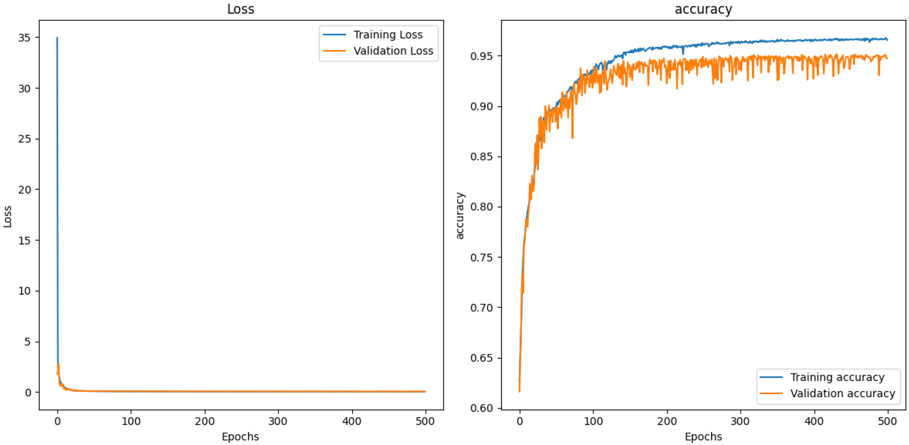
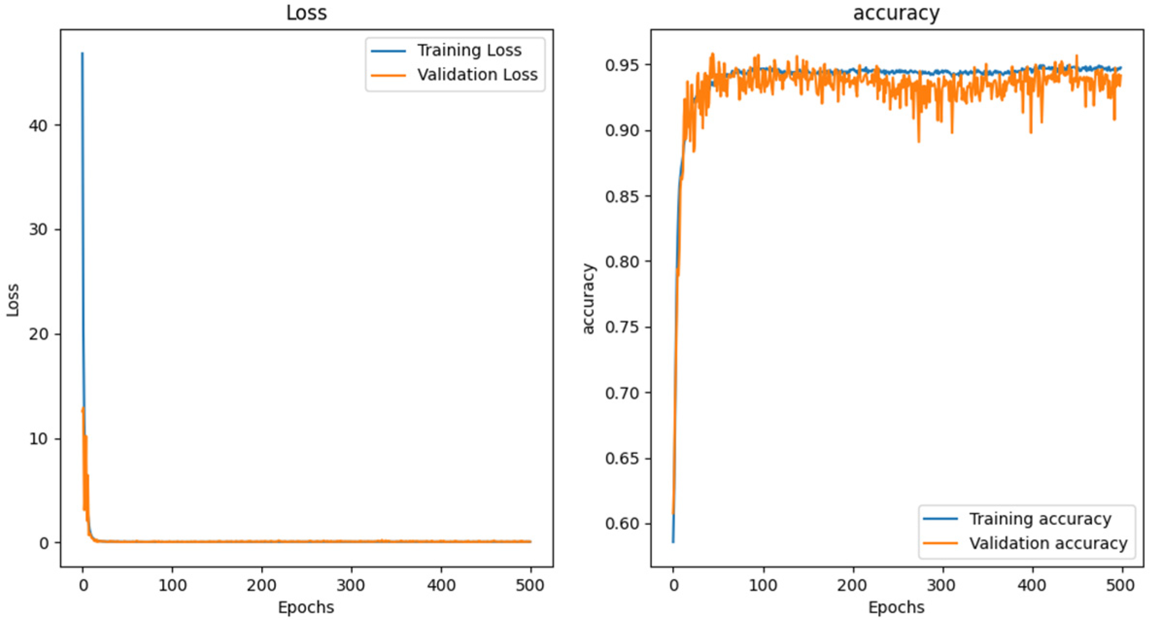
3.4.2. Loss Function and Classification Accuracy

When using the SCNN for data comparison, the model’s predicted value needs to be compared with the true label. During training, positive samples should exhibit a higher similarity, while negative samples should have as low a similarity as possible. The contrastive loss function [33] is commonly used in Siamese networks to guide meaningful feature representation learning by comparing similarities between positive and negative sample pairs. The ${\mathrm{L}\mathrm{o}\mathrm{s}\mathrm{s}}_{\mathrm{c}\mathrm{o}\mathrm{n}\mathrm{t}\mathrm{r}\mathrm{a}\mathrm{s}\mathrm{t}\mathrm{i}\mathrm{v}\mathrm{e}}$ can be expressed as follows:

$${\mathrm{L}\mathrm{o}\mathrm{s}\mathrm{s}}_{\mathrm{c}\mathrm{o}\mathrm{n}\mathrm{t}\mathrm{r}\mathrm{a}\mathrm{s}\mathrm{t}\mathrm{i}\mathrm{v}\mathrm{e}}\left(y,d\right)={\displaystyle \frac{1}{2N}}\sum _{i=1}^N(y_i\cdot d_i^2+(1-y_i)\cdot \mathit{max}(0,margin-d_i{)}^2))$$

(11)

where $y$ represents the true label (positive sample pair labeled as 1, negative sample pair as 0) and $d$ denotes the predicted distance. Meanwhile, $margin$ is a constant determining the separation between different classes of elements, usually set to 1, and $N$ stands for the number of samples.

When the true label $y=1$ represents a positive sample, the loss function is $d^2$, signifying the square of the predicted distance. The loss function promotes similarity by minimizing the distance between their feature representations. When the true label $y=0$, represents a negative sample, the loss function is $max(0,margin-d{)}^2$, namely when predicting a small $margin$ or loss of $(margin-d{)}^2$; otherwise, the loss is 0. Contrastive loss promotes the reduction of similarity by minimizing the square of their distance from the $margin$.

Subsequently, the classification accuracy rate is established and utilized in conjunction with the contrastive loss function:

$$Accuracy={\displaystyle \frac{1}{N}}\sum _{i=1}^N(y_{true,i}=round(y_{pred,i}))$$

(12)

where $N$ is the number of samples, $y_{true,i}$ is the actual label of the i sample, $(y_{pred,i})$ is the prediction probability label for the i sample, the $round$ function maps the probability to the nearest integer (0 or 1).

3.4.3. Similarity Score Function

The similarity score function is determined by the following Euclidean distance metric:

$$similarity scores={\displaystyle \frac{1}{1+e^{k\cdot \frac{distances}{d_{max}}}}}$$

(13)

where $distances$ represents the Euclidean distance between the true label and the model’s prediction. $k$ is the parameter that controls the slope and is usually set to 1. $d_{max}$ is the maximum distance value and is used for normalization, and ${\displaystyle \frac{distances}{d_{max}}}$ is a normalized distance. When two data pieces are closer, the normalization distance is closer to 0, and the similarity score is closer to 0.5. This function is a monotonically decreasing function; so, we can use the maximum similarity score as the criterion for the similarity of two data pieces.

4. Experiments and Results

Section 4 encompasses the execution of experiments and the evaluation of results. Initially, the performance measures for the classification algorithm and the experimental results from classifying the network designed in this paper using the spectrum data set are presented. Subsequently, we discuss the experiment results of the CO₂ feature vector-based classifier method and direct the input of the mid-infrared spectrum into the SCNN. Finally, ablation experiments are provided to compare the effectiveness of peak features, the SCNN model, optimizer selection, learning rate selection, and running time.

4.1. Performance Measures and Experiment Results

Based on the evaluation criteria for data classification tasks, the performance measures of the PF-SCNN for aero-engine hot jet include accuracy, precision, recall, F1-score, and confusion matrix. An instance is classified as a positive class and predicted to be positive, resulting in a True Positive (TP); if it is classified as negative but predicted as positive, it becomes a False Negative (FN); conversely, if the instance is a negative class and predicted to be positive, it results in a False Positive (FP), while predicting negative correctly leads to a True Negative (TN). Based on these assumptions, the evaluation criteria such as accuracy rate, recall rate, F1 value, and confusion matrix are defined as follows:

Accuracy: the accuracy is the ratio of correctly classified samples to the total number of samples.

$$Accuracy={\displaystyle \frac{TP+TN}{TP+TN+FP+FN}}$$

(14)

Precision: the precision is the ratio of correctly predicted positive samples to all predicted positive samples.

$$Precision={\displaystyle \frac{TP}{TP+FP}}$$

(15)

Recall: the recall is the ratio of the number of samples correctly predicted to be positive to the number of samples that are actually positive.

$$Recall={\displaystyle \frac{TP}{TP+FN}}$$

(16)

F1-score: the F1-score is a composite measure of precision and recall, which considers both aspects to evaluate the overall performance of the model.

$$F1-score={\displaystyle \frac{2^{\ast }{P}^{\ast }R}{P+R}}$$

(17)

where $P$ stands for $Precision$, and $R$ stands for $Recall$.

Confusion matrix: the confusion matrix presents the classification results of various categories by the classifier, encompassing TP, FP, TN, and FN. It visually demonstrates the disparity between actual and predicted values, with the diagonal elements indicating the number of accurate predictions for each category made by the classifier.

Table 4. Confusion matrix.

		Forecast Results
		Positive Samples	Negative Samples
Real results	Positive samples	TP	TN
	Negative samples	FP	FN

offers a detailed breakdown of each component in the confusion matrix.

To validate the algorithm’s effectiveness, training and prediction experiments were conducted on a data set comprising six types of aero-engine spectra. The experiments took place on a Windows 10 workstation equipped with 32 GB of RAM, an Intel Core i7–8750H processor, and a GeForce RTX 2070 graphics card.

Table 5. PF-SCNN model parameter information table.

Methods	Parameter Settings
PF-SCNN	Conv1D (32, 3), Conv1D (64, 3), Conv1D (128, 3), activation = ‘relu’
	MaxPooling1D (2) (x)
	Dense (128, activation = ‘relu’)
	Optimizers = RMSProp, (learning_rate = 0.0001)
	Loss = contrastive_loss, metrics = [accuracy]
	Epochs = 500

provides detailed parameters for the PF-SCNN:

According to the parameters in Table 5, we conducted training and label prediction on the data set, and obtained experimental results, as shown in

Table 6. Experiment results of the spectrum matching classification network PF-SCNN.

Evaluation Criterion	Accuracy	Precision	Recall	Confusion Matrix	F1-Score
Data set	99.46%	99.77%	99.56%	[27  0  0  0  0  0] [ 0 72  0  0  0  0] [ 0  0 21  0  0  0] [ 0  1  0 37  0  0] [ 0  0  0  0 20  0] [ 0  0  0  0  0  6]	99.66%

and Figure 5.

The PF-SCNN, as designed in this paper, effectively classifies the spectrum data set of the six types of aero-engine hot jets with a 99.46% accuracy. The model demonstrates high precision (99.77%) and recall (99.56%) values, accurately predicting both positive classes and actual positive samples. The confusion matrix provides insights into prediction performance for each class. The analysis of the F1-score (99.66%) shows a strong balance between accuracy and recall, while loss and accuracy converge rapidly within 500 training sessions—taking 2757.8 s for training and 71 s for label prediction per data point. The accuracy of the model exceeded 90% within 100 epochs, and the classification accuracy of the subsequent training set still increased and exceeded 95%. The validation set showed slight fluctuations, but the classification accuracy also approached 95%.

Despite encountering special cases such as aero-engine failure during the experiment, our PF-SCNN demonstrates robustness with minimal impact on the overall classification accuracy when handling error data within the spectrum data set.

4.2. The Traditional Method Classifies and Compares Experimental Results

The hot jet comprises mixed gases such as oxygen (O₂), nitrogen (N₂), carbon dioxide (CO₂), steam (H₂O), and carbon monoxide (CO), among others. To facilitate comparison with classical classifier methods, the main components of the aero-engine hot jet were analyzed, and a CO₂ feature vector was designed. In the experiment, four characteristic peaks in the mid-infrared region of the BTS from the aero-engine hot jet were selected to construct the spectrum feature vector. These peaks corresponded to wave numbers 2350 cm⁻¹, 2390 cm⁻¹, 720 cm⁻¹, and 667 cm⁻¹, respectively; their positions are illustrated in Figure 6:

The peak differences between 2390 cm⁻¹ and 2350 cm⁻¹, as well as between 719 cm⁻¹ and 667 cm⁻¹, form a single spectral feature vector $a=[a_1,a_2]$:

$$\begin{array}{c}{a}_1=T_{v=2390{cm}^{-1}}-T_{v=2350{cm}^{-1}}\\ a_2=T_{v=719{cm}^{-1}}-T_{v=667{cm}^{-1}}\end{array}$$

(18)

Due to environmental influences, the peak positions of the selected characteristic peaks may shift. The experimentally measured infrared spectrum data’s maximum and minimum peaks at 2350 cm⁻¹, 2390 cm⁻¹, 720 cm⁻¹, and 667 cm⁻¹ are extracted within a specified region to form the spectrum feature vector. The specific threshold range is detailed in

Table 7. Value range of the characteristic peak threshold.

Characteristic Peak Type	Emission Peak (cm−1)			Absorption Peak (cm−1)
Standard feature peak value	2350	2390	720	667
Feature peak range value	2350.5–2348	2377–2392	722–718	666.7–670.5

:

The feature vector needs to be combined with the classifier to test the classification effect. We select commonly used classifiers such as SVM, XGBoost, CatBoost, AdaBoost, Random Forest, LightGBM, and the neural network algorithm and combine them with the CO₂ feature vector for the aero-engine hot jet spectrum classification task.

Table 8. Parameters of CO₂ feature vector classifier methods.

Methods	Parameter Settings
SVM	decision_function_shape = ‘ovr’, kernel = ‘rbf’
XGBoost	objective = ‘multi:softmax’, num_classes = num_classes
CatBoost	loss_function = ‘MultiClass’
Adaboost	n_estimators = 200
Random Forest	n_estimators = 300
LightGBM	objective’: ‘multiclass’, ‘num_class’: num_classes
Neural Network	hidden_layer_sizes = (100), activation = ‘relu’, solver = ‘adam’, max_iter = 200

provides the parameter settings of the classifier algorithms:

In order to compare with the deep learning method, we combine the training set with the validation set, set the training set and the prediction set with a ratio of 9:1, and obtain the experiment results, as shown in

Table 9. Experiment results of CO₂ feature vector classifier methods on spectrum data set.

	Evaluation Criterion	Accuracy	Precision Score	Recall	Confusion Matrix	F1-Score
Classification Methods
CO2 feature vector + SVM		59.78%	44.15%	47.67%	[ 8  0  3  0  0  0] [ 0  3  0  0  0  0] [ 9  1 12  0  0  0] [ 0  3  1 84 22 33] [ 0  0  0  0  0  0] [ 0  0  0  0  0  0]	42.38%
CO2 feature vector + XGBoost		94.97%	92.44%	93.59%	[15  0  3  0  0  0] [ 0  7  0  0  0  0] [ 2  0 13  0  0  0] [ 0  0  0 83  3  0] [ 0  0  0  1 19  0] [ 0  0  0  0  0 33]	92.95%
CO2 feature vector + CatBoost		94.41%	90.35%	93.52%	[15  0  2  0  0  0] [ 0  6  0  0  0  0] [ 2  0 14  0  0  0] [ 0  0  0 83  4  0] [ 0  1  0  1 18  0] [ 0  0  0  0  0 33]	91.81%
CO2 feature vector + AdaBoost		79.89%	63.66%	71.49%	[17  5  6  0  0  0] [ 0  2  0  0  0  0] [ 0  0 10  0  0  0] [ 0  0  0 84 18  3] [ 0  0  0  0  0  0] [ 0  0  0  0  4 30]	62.56%
CO2 feature vector + Random Forest		94.41%	91.40%	92.70%	[15  0  4  0  0  0] [ 0  7  0  0  0  0] [ 2  0 12  0  0  0] [ 0  0  0 83  3  0] [ 0  0  0  1 19  0] [ 0  0  0  0  0 33]	91.91%
CO2 feature vector + LightGBM		94.41%	90.68%	92.40%	[14  0  2  0  0  0] [ 0  6  0  0  0  0] [ 3  0 14  0  0  0] [ 0  0  0 82  2  0] [ 0  1  0  2 20  0] [ 0  0  0  0  0 33]	91.42%
CO2 feature vector + Neural Networks		84.92%	76.79%	76.57%	[17  0  2  0  0  0] [ 0  6  0  0  0  0] [ 0  0 12  0  0  0] [ 0  0  2 84 18  0] [ 0  1  0  0  0  0] [ 0  0  0  0  4 33]	76.02%

:

Based on the analysis of the experimental results for the CO₂ feature vector classifier methods, it is observed that the overall performance of the SVM algorithm in the classification task is suboptimal. AdaBoost exhibits poor prediction performance with consistently low indices. while the neural networks also underperform. Conversely, XGBoost, CatBoost, Random Forest, and LightGBM demonstrate strong classification capabilities with an excellent predictive accuracy, a positive instance capture, and a balanced accuracy rate and recall rate. However, they still have some distance from our high-precision recognition. This distance is reflected in the limitation of a single feature vector to the feature representation of data. In complex experimental scenarios, it is not enough to use CO₂ as a single spectrum feature to represent the spectrum characteristics, and more features should be explored to describe our spectrum data.

4.3. Ablation Experiment Analysis

4.3.1. Peak Feature Effectiveness

Integrating peak features with traditional classifiers validates their impact on algorithm enhancement for classification. We identified peaks in our data set and obtained experimental results, as depicted in Figure 7:

In Figure 7a,c, the curves represent all the spectra in the data set. In Figure 7a, the red points represent all peak points identified by the peak-finding algorithm; in Figure 7b, the blue histogram illustrates the distribution of these peak positions within the data set; and in Figure 7c, the red line denotes the wavenumber position of the high-frequency peak, and its intersection with the spectral curve corresponds to the peak point. Following a comprehensive statistical analysis of these peak positions, a total of 56 peaks were identified. Subsequently, data corresponding to these 56 peak positions from each data set were computed, and a classification experiment was conducted using SVM and XGBoost classifier methods as part of our previous study, resulting in detailed classification results, which are presented in

Table 10. Experiment results of peak-seeking classifier on spectral data set.

Methods	Accuracy	Precision	Recall	Confusion Matrix	F1-Score	Running Time
Peaks + SVM	58.15	48.09	43.58	[ 0  0  0  0  0  0] [13 42  0  0  0  0] [ 0  0 20  0 13  6] [14 30  0 38  0  0] [ 0  0  1  0  7  0] [ 0  0  0  0  0  0]	41.02	0.54
Peaks + XGBoost	98.91	96.78	99.01	[27  0  0  0  0  0] [ 0 72  0  1  0  0] [ 0  0 21  0  0  1] [ 0  0  0 37  0  0] [ 0  0  0  0 20  0] [ 0  0  0  0  0  5]	97.76	1.27

:

Comparing the data in Table 9, the peak and SVM classification results are similar to CO₂, while the peak improves the classification accuracy of XGBoost. It can be said that the peak is helpful for improving the classification results. The experimental findings suggest that feature extraction using the peak-finding algorithm is highly effective for classification tasks.

4.3.2. SCNN Model

We use the same parameters of the PF-SCNN model to input data in the mid-infrared region into the SCNN for training and prediction, and obtain

Table 11. Experiment results of spectrum matching classification SCNN model.

Evaluation Criterion	Accuracy	Precision	Recall	Confusion Matrix	F1-Score
Data set	99.46%	99.24%	99.56%	[27  0  0  0  0  0] [ 0 72  0  0  0  0] [ 0  0 21  0  0  0] [ 0  0  1 37  0  0] [ 0  0  0  0 20  0] [ 0  0  0  0  0  6]	99.39%

and Figure 8:

The SCNN performs well on all evaluation metrics, but its precision and F1-score are slightly lower compared to the PF-SCNN model. From the confusion matrix analysis, there is a misclassification in category 4. However, it is unsatisfactory that the training time of the SCNN model is 19,103.60 s when using the entire mid-infrared spectrum as the input. In terms of model training, the model can achieve a classification accuracy of 90% within 100 epochs, and the loss function converges quickly. Although there is a slight fluctuation in the validation set, the training set curve changes very stably. Compared to the training performance of the PF-SCNN, the SCNN is slightly inferior, but overall it performs very well. It is evident that the SCNN model can achieve commendable accuracy in both training and prediction. However, owing to data quantity issues, the SCNN model demands substantial computing resources and time.

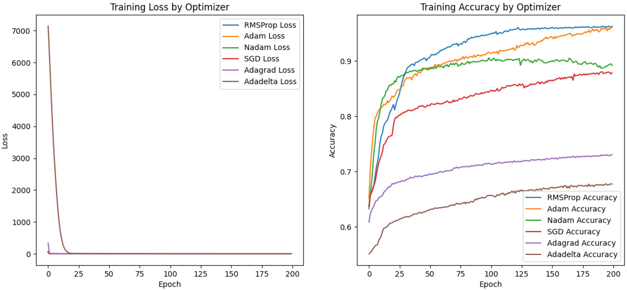
4.3.3. Optimizer Selection

In deep learning network training, we input commonly used optimizers such as RMSProp, Adam, Nadam, SGD, Adagrad, and Adadelta into the base network model for comparison on the spectrum data used in this paper to determine the most suitable optimizer. The optimizer parameters are shown in

Table 12. Optimizer parameters information.

Methods	Parameter Settings
RMSProp	learning rate = 0.0001, clipvalue = 1.0
Adam	learning rate = 0.0001, clipvalue = 1.0
Nadam	learning rate = 0.0001, clipvalue = 1.0
SGD	learning rate = 0.0001, clipvalue = 1.0
Adagrad	learning rate = 0.0001, clipvalue = 1.0
Adadelta	learning rate = 0.0001, clipvalue = 1.0

:

We conducted 200 training tests on the peak data of the spectrum data set using various optimizers on the base network, and the results are shown in

Table 13. Experiment results of different optimizers.

Optimizers	Prediction Accuracy	Training Time/s
RMSProp	96%	1180.96
Adam	96%	1014.82
Nadam	89%	1523.14
SGD	88%	1101.65
Adagrad	73%	1021.90
Adadelta	68%	991.90

and Figure 9:

RMSProp and Adam perform the best in terms of prediction accuracy, and Adam has the shortest training time, thus achieving a good balance between prediction accuracy and training time. Although Nadam has a slightly lower prediction accuracy, it takes the longest training time, which may indicate that it requires more iterations during the training process. The prediction accuracy and training time of the SGD are both at a moderate level. Adagrad and Adadelta perform poorly in terms of prediction accuracy, especially Adadelta, but their training time is relatively short. As depicted in the graph, both RMSProp and Adam exhibit rapid convergence on the loss function curve and accuracy curve after 200 iterations of model training, leading to high prediction accuracy. Under the premise of prioritizing prediction accuracy, RMSProp is a more suitable choice for the model in this article.

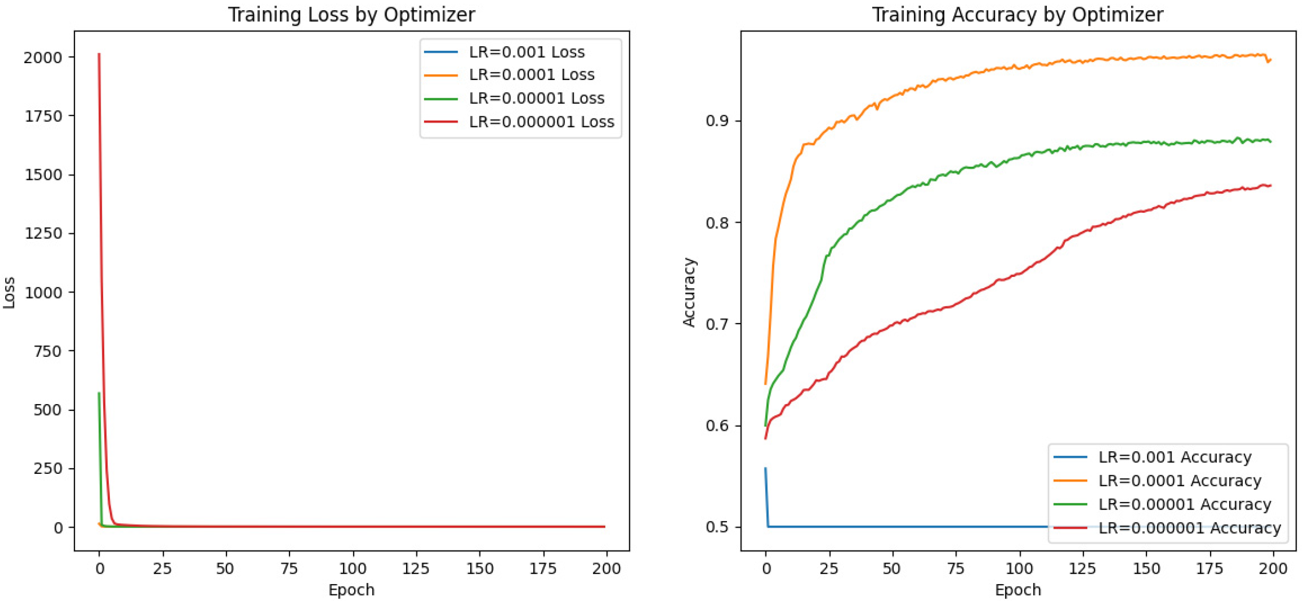
4.3.4. Learning Rate Selection

The choice of the learning rate is a crucial step in training a neural network. In our experiments, we tried different learning rate values and observed their impact on the model’s performance. Starting from 0.001, we gradually increased the learning rate using a power of 10. In this way, we obtained a series of results and summarized them in

Table 14. Experiment results of RMSProp optimizer in different learning rate.

Learning Rate	Prediction Accuracy	Training Time/s
0.001	0.50	1283.49
0.0001	0.96	1252.83
0.00001	0.88	1171.39
0.000001	0.84	1193.72

and Figure 10 for a detailed comparison and analysis. This helps us to find the optimal learning rate value that best fits the data set and model architecture, thereby improving training efficiency and model performance:

When the learning rate is 0.001, the prediction accuracy is the lowest, only 0.50. As the learning rate decreases (0.0001), the prediction accuracy significantly improves to 0.96. Further reducing the learning rate (0.00001 and 0.000001) resulted in a decrease in prediction accuracy, with values of 0.88 and 0.84, respectively. This indicates that the choice of the learning rate has a significant impact on the prediction accuracy of the model. An excessively high learning rate may cause the model to fail to converge, while an excessively low learning rate may result in a slow update speed when approaching the optimal solution, thereby affecting the final prediction accuracy. In terms of time, this indicates that a decrease in the learning rate typically reduces the training time, but a learning rate that is too low may lead to an increase in training time, as the model requires more iterations to converge.

Based on the variations in the loss function and accuracy curves for a given optimizer under different learning rates, as well as considering the final accuracy value, it is apparent that RMSProp demonstrates optimal performance on the spectrum data set when utilizing a learning rate of 0.0001. This is consistent with the learning rate we have adopted.

4.3.5. Running Time

Deep learning methods necessitate longer model training times due to their typical utilization of large data sets and complex network structures. In contrast to traditional classifier methods, deep learning algorithms require more iterations for parameter adjustment and model optimization in order to achieve a higher accuracy and generalization capability. In practical applications, we conducted a detailed comparison of prediction times for different methods on data sets and compiled the results into a test time comparison table, as shown in

Table 15. Prediction time comparison.

Methods	Prediction Time
PF-SCNN	71 s Each data; 3:44:17 total
SCNN	79 s Each data; 4:30:45.78 total
CO2 feature vector + SVM	0.12 s
CO2 feature vector + XGBoost	0.30 s
CO2 feature vector + CatBoost	4.74 s
CO2 feature vector + AdaBoost	0.39 s
CO2 feature vector + Random Forest	0.56 s
CO2 feature vector + LightGBM	0.44 s
CO2 feature vector + Neural Networks	0.85 s

. These data clearly illustrate the differences in prediction times required by various algorithms when processing the same data set, providing valuable references for further analysis and evaluation:

The data in Table 15 indicate that CO₂ feature vector classifiers exhibit fast running times. However, the PF-SCNN does not offer significant advantages in terms of running time, as it requires matching prediction data with trained data during the network’s prediction stage, resulting in the substantial consumption of computing time and memory. Although introducing peak values significantly enhances algorithmic speed compared to only using the SCNN model for prediction, the one-to-one matching method still demands considerable computing time. Based on these findings regarding running times, our future research will focus on extracting stable and distinct features from each type of aero engine’s hot jet spectrum to reduce the predicted data volume and prediction time.

In summary, the CO₂ feature vector can achieve a high classification accuracy with excellent classification algorithms such as XGBOOST, Random Forest, and LightGBM, and complete the classification task in a short time. However, the stability of spectral classification for aviation engines based on single features is questionable in the face of complex environmental factors. In comparison, the PF-SCNN has a greater potential to tackle spectral classification problems in complex environments, but the disadvantage is that the prediction stage chose a strategy of matching one by one, resulting in a longer prediction time. For this problem, the focus of future research will be on the study of the features of each type of aero-engine, deeply mining the potential features of each type of aero-engine, and preparing for the subsequent spectral data of more types of aero-engines.

5. Conclusions

The PF-SCNN with a dual-branch structure proposed in this paper is designed for matching and classifying spectrum data. It utilizes the peak-finding algorithm to extract spectrum peak values, which are then input to the SCNN for spectrum feature extraction and distance similarity calculation. The experimental results demonstrate a high prediction accuracy of 99%, validating the effectiveness of the PF-SCNN in achieving good matching with the spectrum data set and its successful application in classifying the hot jet spectra of aero-engines. However, the method’s approach of individually matching each test data with all trained data during the prediction stage leads to significant time and computational costs. Future iterations of this algorithm should prioritize extracting representative characteristic peaks from each type of aero-engine’s hot jet spectrum data and identifying prominent features within each category. Subsequently, the PF-SCNN can be employed to compare predicted data with representative characteristic peak data, thereby enhancing classification accuracy and matching rates.

References

1. Rozenstein, O.; Puckrin, E.; Adamowski, J. Development of a new approach based on midwave infrared spectroscopy for post-consumer black plastic waste sorting in the recycling industry. Waste Manag. 2017, 68, 38–44. [Google Scholar] [CrossRef] [PubMed]
2. Hou, X.; Lv, S.; Chen, Z.; Xiao, F. Applications of Fourier transform infrared spectroscopy technologies on asphalt materials. Measurement 2018, 121, 304–316. [Google Scholar] [CrossRef]
3. Ozaki, Y. Infrared Spectroscopy—Mid-infrared, Near-infrared, and Far-infrared/Terahertz Spectroscopy. Anal. Sci. 2021, 37, 1193–1212. [Google Scholar] [CrossRef]
4. Jang, H.-D.; Kwon, S.; Nam, H.; Chang, D.E. Semi-Supervised Autoencoder for Chemical Gas Classification with FTIR Spectrum. Sensors 2024, 24, 3601. [Google Scholar] [CrossRef]
5. Uddin, M.P.; Mamun, M.A.; Hossain, M.A. PCA-based Feature Reduction for Hyperspectral Remote Sensing Image Classification. IETE Tech. Rev. 2021, 38, 377–396. [Google Scholar] [CrossRef]
6. Xia, J.; Bombrun, L.; Adali, T.; Berthoumieu, Y.; Germain, C. Spectral–Spatial Classification of Hyperspectral Images Using ICA and Edge-Preserving Filter via an Ensemble Strategy. IEEE Trans. Geosci. Remote Sens. 2016, 54, 4971–4982. [Google Scholar] [CrossRef]
7. Jia, S.; Zhao, Q.; Zhuang, J.; Tang, D.; Long, Y.; Xu, M.; Zhou, J.; Li, Q. Flexible Gabor-Based Superpixel-Level Unsupervised LDA for Hyperspectral Image Classification. IEEE Trans. Geosci. Remote Sens. 2021, 59, 10394–10409. [Google Scholar] [CrossRef]
8. Zhang, Y.; Li, T. Three different SVM classification models in Tea Oil FTIR Application Research in Adulteration Detection. In Journal of Physics: Conference Series; IOP Publishing: Bristol, UK, 2021; Volume 1748, p. 022037. [Google Scholar]
9. Chen, T.; Guestrin, C. XGBoost: A scalable tree boosting system. In Proceedings of the 22nd Acm Sigkdd International Conference on Knowledge Discovery and Data Mining, San Francisco, CA, USA, 13–17 August 2016; pp. 785–794. [Google Scholar]
10. Breiman, L. Random Forests. Mach. Learn. 2001, 45, 5–32. [Google Scholar] [CrossRef]
11. Kumaravel, A.; Muthu, K.; Deenadayalan, N. A View of Artificial Neural Network Models in Different Application Areas. E3S Web Conf. 2021, 287, 03001. [Google Scholar]
12. Li, X.; Li, Z.; Qiu, H.; Hou, G.; Fan, P. An overview of hyperspectral image feature extraction, classification methods and the methods based on small samples. Appl. Spectrosc. Rev. 2021, 58, 367–400. [Google Scholar] [CrossRef]
13. Chen, Y.; Lin, Z.; Zhao, X.; Wang, G.; Gu, Y. Deep Learning-Based Classification of Hyperspectral Data. IEEE J. Sel. Top. Appl. Earth Obs. Remote Sens. 2014, 7, 2094–2107. [Google Scholar] [CrossRef]
14. Zhou, W.; Kamata, S.-I.; Wang, H.; Xue, X. Multiscanning-Based RNN–Transformer for Hyperspectral Image Classification. IEEE Trans. Geosci. Remote. Sens. 2023, 61, 1–19. [Google Scholar] [CrossRef]
15. Hu, H.; Xu, Z.; Wei, Y.; Wang, T.; Zhao, Y.; Xu, H.; Mao, X.; Huang, L. The Identification of Fritillaria Species Using Hyperspectral Imaging with Enhanced One-Dimensional Convolutional Neural Networks via Attention Mechanism. Foods 2023, 12, 4153. [Google Scholar] [CrossRef] [PubMed]
16. Ma, Y.; Lan, Y.; Xie, Y.; Yu, L.; Chen, C.; Wu, Y.; Dai, X. A Spatial–Spectral Transformer for Hyperspectral Image Classification Based on Global Dependencies of Multi-Scale Features. Remote Sens. 2024, 16, 404. [Google Scholar] [CrossRef]
17. Jia, S.; Jiang, S.; Lin, Z.; Xu, M.; Sun, W.; Huang, Q.; Zhu, J.; Jia, X. A Semisupervised Siamese Network for Hyperspectral Image Classification. IEEE Trans. Geosci. Remote. Sens. 2021, 60, 1–17. [Google Scholar] [CrossRef]
18. Ondrasovic, M.; Tarabek, P. Siamese Visual Object Tracking: A Survey. IEEE Access 2021, 9, 110149–110172. [Google Scholar] [CrossRef]
19. Xu, T.; Feng, Z.; Wu, X.-J.; Kittler, J. Toward Robust Visual Object Tracking With Independent Target-Agnostic Detection and Effective Siamese Cross-Task Interaction. IEEE Trans. Image Process. 2023, 32, 1541–1554. [Google Scholar] [CrossRef]
20. Wang, L.; Wang, L.; Wang, Q.; Atkinson, P.M. SSA-SiamNet: Spectral–Spatial-Wise Attention-Based Siamese network for Hyperspectral Image Change Detection. IEEE Trans. Geosci. Remote Sens. 2022, 60, 1–18. [Google Scholar] [CrossRef]
21. Melekhov, I.; Kannala, J.; Rahtu, E. Siamese network features for image matching. In Proceedings of the 2016 23rd International Conference on Pattern Recognition (ICPR), Cancun, Mexico, 4–8 December 2016. [Google Scholar]
22. Li, Y.; Chen, C.L.P.; Zhang, T. A Survey on Siamese network: Methodologies, Applications, and Opportunities. IEEE Trans. Artif. Intell. 2022, 3, 994–1014. [Google Scholar] [CrossRef]
23. Huang, L.; Chen, Y. Dual-Path Siamese CNN for Hyperspectral Image Classification With Limited Training Samples. IEEE Geosci. Remote Sens. Lett. 2021, 518–522. [Google Scholar] [CrossRef]
24. Miao, J.; Wang, B.; Wu, X.; Zhang, L.; Hu, B.; Zhang, J.Q. Deep Feature Extraction Based on Siamese network and Auto-Encoder for Hyperspectral Image Classification. In Proceedings of the IGARSS 2019—2019 IEEE International Geoscience and Remote Sensing Symposium, Yokohama, Japan, 28 July–2 August 2019. [Google Scholar]
25. Nanni, L.; Minchio, G.; Brahnam, S.; Maguolo, G.; Lumini, A. Experiments of Image Classification Using Dissimilarity Spaces Built with Siamese Networks. Sensors 2021, 21, 1573. [Google Scholar] [CrossRef]
26. Liu, B.; Yu, X.; Zhang, P.; Yu, A.; Fu, Q.; Wei, X. Supervised Deep Feature Extraction for Hyperspectral Image Classification. IEEE Trans. Geosci. Remote Sens. 2017, 56, 1909–1921. [Google Scholar] [CrossRef]
27. Rao, M.; Tang, P.; Zhang, Z. A Developed Siamese CNN with 3D Adaptive Spatial-Spectral Pyramid Pooling for Hyperspectral Image Classification. Remote Sens. 2020, 12, 1964. [Google Scholar] [CrossRef]
28. Kruse, F.A.; Kierein-Young, K.S.; Boardman, J.W. Mineral mapping at Cuprite, Nevada with a 63-channel imaging spectrometer. Photogramm. Eng. Remote Sens. 1990, 56, 83–92. [Google Scholar]
29. Bromley, J.; Bentz, J.W.; Bottou, L.; Guyon, I.; LeCun, Y.; Moore, C.; Sackinger, E.; Shah, R. Signature Verification using a "Siamese" Time Delay Neural Network. Int. J. Pattern Recognit. Artif. Intell. 1993, 7, 669–688. [Google Scholar] [CrossRef]
30. Thenkabail, P.; GangadharaRao, P.; Biggs, T.; Krishna, M.; Turral, H. Spectral Matching Techniques to Determine Historical Land-use/Land-cover (LULC) and Irrigated Areas Using Time-series 0.1-degree AVHRR Pathfinder Datasets. Photogramm. Eng. Remote Sens. 2007, 73, 1029–1040. [Google Scholar]
31. Sohn, K. Improved deep metric learning with multi-class N-pair loss objective. In Advances in Neural Information Processing Systems; MIT Press: Cambridge, MA, USA, 2016; pp. 1857–1865. [Google Scholar]
32. Homan, D.C.; Cohen, M.H.; Hovatta, T.; Kellermann, K.I.; Kovalev, Y.Y.; Lister, M.L.; Popkov, A.V.; Pushkarev, A.B.; Ros, E.; Savolainen, T. MOJAVE. XIX. Brightness Temperatures and Intrinsic Properties of Blazar Jets. Astrophys. J. 2021, 923, 67. [Google Scholar] [CrossRef]
33. Zhou, W.; Zhang, J.; Jie, D. The research of near infrared spectral peak detection methods in big data era. In Proceedings of the 2016 ASABE International Meeting, Orlando, FL, USA, 17–20 July 2016. [Google Scholar]
34. Tieleman, T.; Hinton, G. Lecture 6.5-rmsprop: Divide the gradient by a running average of its recent magnitude. Coursera Neural Netw. Mach. Learn. 2012, 4, 26–31. [Google Scholar]
Figure 1. Aero-engine hot jet infrared spectrum measurement experiment site layout diagram.
Aerospace 11 00703 g001
Figure 2. Experiment measurement of infrared spectra of aero-engine hot jets: the red box represents carbon dioxide, the gray box represents steam and the blue box represents carbon monoxide.
Aerospace 11 00703 g002
Figure 3. Spectrum classification Siamese network infrastructure.
Aerospace 11 00703 g003
Figure 4. Detailed drawing of the aero-engine hot jet infrared spectrum classification network PF-SCNN.
Aerospace 11 00703 g004
Figure 5. PF-SCNN spectrum matching classification experiment results, where the left figure is the loss function transformation curve, the right figure is the correct rate transformation curve, the blue line is the training data, and the orange line is the verification data.
Aerospace 11 00703 g005
Figure 6. The position diagram of the four characteristic peaks of the measured aero-engine.
Aerospace 11 00703 g006
Figure 7. Experimental results of peak-finding and high frequency peak statistics: (a) visualization of peak-finding, (b) statistics of peak frequency, and (c) visualization of peak position.
Aerospace 11 00703 g007aAerospace 11 00703 g007b
Figure 8. SCNN spectrum matching classification experiment results, where the (left) figure is the loss function transformation curve, the (right) figure is the correct rate transformation curve, the blue line is the training data, and the orange line is the verification data.
Aerospace 11 00703 g008
Figure 9. Network training and validation of loss function and accuracy variation curves on spectrum data set by different optimizers: RMSProp in blue, Adam in orange, Nadam in green, SGD in red, Adagrad in purple, and Adadelta in brown.
Aerospace 11 00703 g009
Figure 10. Network training and validation of RMSProp with different learning rates on spectrum data sets loss function and accuracy change curve: Among them, blue represents the learning rate of 0.001, orange represents the learning rate of 0.0001, green represents the learning rate of 0.00001, and red represents the learning rate of 0.000001.
Aerospace 11 00703 g010