Abstract
Runway Safety Assistant Foreseeing Excursions (RUNSAFE) is a complete embedded system solution, that predicts a potential runway overrun of a civil aviation aircraft during takeoff and landing. This work examines the feasibility of such a system, through the algorithms and computations that predict the overruns. The system executes both static and dynamic calculations, with the former being dependent on and the latter independent to the user’s inputs. Their outcomes and the runway’s length are compared in real time to assess if the process will end up in an overrun. All inputs are specifically selected to either be available to the pilots or be retrieved from the existing avionics systems of the cockpit. A performance evaluation is conducted on both static and dynamic calculations, and metrics unveil the accuracy of the predictions and the time needed to converge to a reliable result. The solution is adapted for a Boeing 737-800 aircraft with CFM56-7B engines, but the calculations also apply for similar aircraft equipped with tricycle landing gear and turbofan engines, namely the whole Boeing 737 family, the Airbus A320 family, etc. The system is aligned with current standards and certification specifications, where applicable.
1. Introduction
The most critical stages during a flight are takeoff and landing, as extremely large changes in the kinetic energy of the aircraft happen during these times. The constraints that the length of the runway sets, as well as the existing environmental conditions, make the task even more difficult for the operators, where they have to cope with them, occasionally without alternatives. One of the types of accidents that occurs in these stages leads to exceeding the length of the runway, a type of accident with a low mortality rate. However, it leads to passenger confusion, temporary unavailability of the runway, damage to the aircraft and/or the runway itself, defamation of the airline, and more. Runway overrun incidents in civil aviation occupied the first place in runway-related incidents during the 2010–2014 period [1].
Since the human factor is the leading cause of aviation accidents [2], there should be a system that supports and warns the operators in cases of a potential runway overrun. That way, the risk and occurrences of such incidents can be decreased.
1.1. Calculation of Critical Speeds
Before starting any takeoff or landing procedure, and based on a number of factors, some critical speeds (V1,V2 and VR for takeoff, Vapp and Vref for landing) are derived. Their calculation is performed through the flight manuals of the respective aircraft and recently through software solutions (e.g., Flysmart+ [3]). The first ones produce approximate calculations with large margins of error, while software calculations are more precise, including safety margins. The scope of these speed indicators is to complete each process with safety and prevent the airplane from overshooting the runway. At the same time, acceleration and deceleration rates that occur prevent the straining of the aircraft’s mechanisms and provide comfort to the passengers.
1.2. Motivation
The motivation for developing the RUNSAFE system arises from the need to address significant safety concerns in civil aviation, particularly related to runway overruns during takeoff and landing. Runway overruns, although generally having a low mortality rate, can lead to severe consequences, including aircraft damage, operational disruptions, and economic losses. This issue has been highlighted in the European Union Aviation Safety Agency’s (EASA) research agenda for 2022–2024, which specifically calls for innovations to assist flight crews in preventing runway overruns and managing aircraft energy during critical flight phases [4] (LOC-03).
Recent statistics show that runway overruns were the most common runway-related incident in civil aviation between 2010 and 2014 [1]. Given the high frequency and potential impact of these incidents, there is a clear and urgent need for systems that can provide real-time predictive warnings to pilots. The RUNSAFE. system is designed to fulfill this need by offering a decision support tool that can dynamically calculate and predict the likelihood of a runway overrun, thereby enhancing safety and reducing the risk of such incidents. By developing this system, we aim to contribute to the broader goal of improving runway safety and aligning with EASA’s research priorities.
1.3. Assumptions
The statically calculated critical speeds assume the smooth development of the procedures. In particular, it is assumed that during takeoff the engines perform at 100%. Also, during landing, it is assumed that the aircraft comes in contact with the ground before a certain point, and that the friction between the wheels and the runway is exactly as predicted. Although major deviation factors are easily observable by operators (e.g., engine loss, flat tire), others are not that obvious (e.g., reduced engine performance due to need for regular maintenance, worn tires), while in other cases operators misjudge the capabilities of the aircraft.
This is due to the inherent inability of predicting anomalies during the evolution of the process, such as those mentioned above. This also leads to the second cause, which is that values extracted from the static calculations correspond to velocities, while the main limiting factor is the length of the runway. Even though an aircraft’s instruments indicate the aircraft’s speed accurately, there is no indication of its position relative to the runway, and the crew can only derive conclusions by the visual contact they have with it. This is where the experience of the pilots must contribute to assessing whether the remaining runway is sufficient to bring the aircraft to a full stop. However, such a thing is practically impossible to calculate precisely.
1.4. System Specifications
Based on the above, it is understandable that there is a need for an auxiliary decision support system that belongs in the aircraft’s cockpit and is able to calculate the point at which critical speeds are attained on the runway, the most important being the point at which the aircraft is expected to come to a full stop. The system must be able to perform two different calculations, a static and a dynamic one.
The static calculation is based excursively on users’ inputs and aims to calculate the distance needed in each procedure. For takeoff, the Accelerate Stop Distance Required (ASDR) is calculated, while during landing the corresponding distance is the Landing Distance Required (LDR). Such calculations cannot take into account real-world interference, thus, no matter how precise the calculation is, it is not able to predict unexpected events and/or the actual deviation. This is why real-time/online algorithms are a necessity.
The dynamic calculation starts when the acceleration of the aircraft is initiated during takeoff and at a certain height in the case of landing. The calculations are based solely on factors other than user inputs, such as acceleration, velocity, height from the ground, etc.
1.5. Obtaining Necessary Data
All the static calculations mentioned previously require data regarding the aerodynamic characteristics of the aircraft, the performance of the engines, and the interaction with the surrounding environment. Few to no data are available online concerning the aircraft and, even if there are, data verification is required. For this purpose, the flight simulator X-Plane 11 is used, which provides both the necessary data and the verification framework for the correct operation of the system. This particular simulator is chosen based on its ability to represent the real world as closely as possible to the laws of physics.
To interact and retrieve these values from the simulator, a suitable code has been developed in Python 3.11.2. The integrated UDP sends the user-selected information in packets. These packets are sent on every new calculation the simulator makes, i.e., every new frame. The data are either processed or stored, depending on the use for which they are intended. The data fields sampled from the simulator can be found analytically in Appendix A.
2. State of the Art
The specifications of a Takeoff Performance Monitoring System (TOPMS) were defined for the first time in August of 1987, in the AS-8044 standard (Aerospace Standard 8044), and were modified in 2007 and 2020 [5]. Three types of such systems are defined, depending on their function. These are:
- Type 1: non-predictive systems, only compare actual to expected performance;
- Type 2: prediction of the takeoff distance;
- Type 3: prediction of the takeoff distance and braking distance in case of abort.
Although a TOPMS prototype has been developed by NASA [6] and other organizations, there is no system widely used in aviation. EASA took the initiative to set up a study group (Working Group 88), exclusively for the study of TOPMS, which in 2017 concluded that such systems are unfeasible due to limitations in technology and data [7].
A recent proposal for a TOPMS came from the Netherlands Aerospace Centre (NLR), in the Takeoff Performance Alerting Program (TOPAP). It only detects and notifies for major errors in the expected and actual acceleration during takeoff, which signifies differences in the actual and given weight during the necessary pre-takeoff calculations and the weight input in the Flight Management System (FMS) [8].
On the other hand, runway excursion alerting systems for landing have been developed and used for more than a decade in commercial aviation. Since 2020, all new aircraft must be equipped with a Runway Overrun Awareness and Alerting System (ROAAS), in order to comply with EASA’s CS-25 Amendment 24 (Certification Specifications for Large Aeroplanes). The two largest aircraft manufacturers, Airbus and Boeing, have developed their own solutions named the Runway Overrun Prevention System (ROPS) and Runway Awareness and Advisory System (RAAS), respectively.
EASA explicitly defines that “The ROAAS shall reduce the risk of a longitudinal runway excursion during landing by providing alert, in flight and on ground, to the flight crew when the aeroplane is at risk of not being able to stop within the available distance to the end of the runway.
- During approach (from a given height above the selected runway) and landing, the ROAAS shall perform real-time energy-based calculations of the predicted landing stopping point, compare that point with the location of the end of the runway, and provide the flight crew with:
- (a)
- in-flight, timely, and unambiguous predictive alert(s) of a runway overrun risk, and
- (b)
- on-ground, timely, and unambiguous predictive alert(s) of a runway overrun risk. At the option of the applicant, the ROAAS may also provide an automated means of deceleration control that prevents or minimizes runway overrun during landing.
- The ROAAS shall at least accommodate dry and wet runway conditions for normal landing configurations [9].
The landing mode of the RUNSAFE system was developed in compliance with the ROAAS definition, apart from Item 1.b of the definition; hence, new aircraft can be equipped with the system, or it can be installed in older aircraft in order to be up to date with the newer regulations. A full adaption to an aircraft will also be able to satisfy Item 1.b, accessing control to automated means of deceleration.
Current runway safety systems, such as the Runway Overrun Prevention System (ROPS), Runway Awareness and Advisory System (RAAS), and Takeoff Performance Monitoring System (TOPMS), have made significant advances but are limited by their reliance on static, pre-calculated data and insufficient integration of real-time environmental and aircraft-specific factors. These limitations hinder their ability to provide accurate and timely predictions of runway excursions, especially under rapidly changing conditions [10]. Additionally, these systems lack the adaptability needed to function effectively across different aircraft models and varying operational scenarios [11,12].
The RUNSAFE system is designed to address these gaps by providing a robust, real-time predictive model that continuously integrates both static and dynamic data to foresee potential runway overruns. Unlike existing systems, RUNSAFE is adaptable to various aircraft models, including the Boeing 737-800, and can be customized for different runway conditions, for both the landing and takeoff procedures. By using real-time inputs such as aircraft acceleration, speed, and environmental conditions, the system dynamically predicts the likelihood of an overrun, offering timely alerts to the flight crew. This unified system represents a significant advancement over existing ones.
3. Takeoff Procedure
Takeoff is defined as the phase during which the aircraft aims to obtain a certain speed that makes it capable of flying under its own lift. However, there are cases where the aircraft encounters problems during this process, leading to potential overruns, if handled with a rejected takeoff (RTO). Factors that can lead to these situations include technical problems with the aircraft’s systems, adverse weather conditions, deficiencies in the execution of takeoff procedures by the crew, and factors affecting runway availability.
In the case of an RTO, the crew must follow certain procedures that aim to stop the aircraft with safety, although at times the overestimation of the crew’s and the aircraft’s abilities can often lead to a runway overrun.
Currently, the standard term that prevents a runway overrun during takeoff is the V1 speed (also referred to as decision speed). This critical speed marks the point beyond which the pilot no longer has the capability to cancel the takeoff procedure, as the remaining length of the airport runway is not sufficient to safely abort the takeoff [13]. Both static and dynamic calculations, executed by the system, estimate the distance needed to accelerate to V1 and then decelerate to a full stop.
3.1. Static Calculations
The fundamental principle for statically calculating distance during the accelerating and the decelerating phases of a rejected takeoff is Newton’s second law, in which the sum of the forces acting on a body is equal to the rate of change of the body’s momentum:
Therefore, by modeling all the forces that act on the aircraft parallel to its longitudinal axis, with sufficient accuracy, its acceleration can be calculated at any given moment. Acceleration’s first integral is velocity, hence the bounds of the integral (time frame) of the accelerating and decelerating part can be found. By integrating once more, within the same bounds, we find the distance covered.
The algorithm that implements this double integral is based on the Riemann sum, in which the definite integral, S, of a function, f, is computed as a sum of area of parallelograms, with the variable of integration, in this case, being time t:
with .
Figure 1 exhibits the algorithm that calculates the distance required to attain a certain speed, that being V1 for acceleration and 0 for deceleration. The velocity and distance variables are initialized to v_init (0 for acceleration and V1 for deceleration) and 0, respectively. For each repetition of the loop, we firstly calculate the sum of forces acting on the axis parallel to the runway, , and we divide with the mass to find acceleration . The following two commands essentially implement a right Riemann sum, and update the values for speed and distance. The loop exits when the final speed is reached.
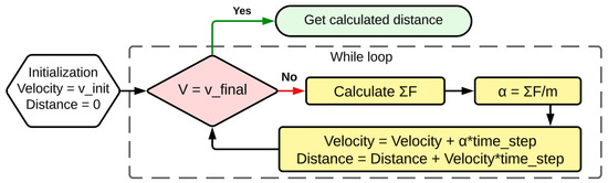
Figure 1.
While loop for calculating distances.
The division (time step) used directly affects the accuracy of the result. By reducing the time step, the accuracy increases as well as the operations needed. For this particular implementation, the golden medium between the two was found to be at 0.05 s, as it leads to instant calculations without sacrificing the accuracy (deviation less than 1 m).
As far as the right Riemann sum is concerned, we found that the time step is of such a scale that switching between the right, left, and middle Riemann sum does not lead to a notable difference to the final result. Hence, the right is chosen, since it needs fewer calculations and the algorithm will be embedded into a resource-limited device.
3.1.1. Forces Acting on the Aircraft
The forces acting on the aircraft, which are parallel to the runway, are those that change the speed of the aircraft. These are the thrust of the engines, , the aerodynamic drag, , the friction between the tires and the runway, , and the component of the weight on the axis of the runway, , which depends on its slope, , as shown in Figure 2.

Figure 2.
Forces acting on the aircraft while on the runway.
Each of the forces is studied separately in the following paragraphs.
Engine Thrust
The Boeing 737-800 has two turbofan CFM56–7B26 type engines. Turbofan engines have expected performance characteristics that depend on altitude and airspeed [14] (p. 592). The diagram for the aircraft’s engines is available in the simulator, as depicted in Figure 3. The produced thrust in the diagram refers to thrust production at 100% N1.
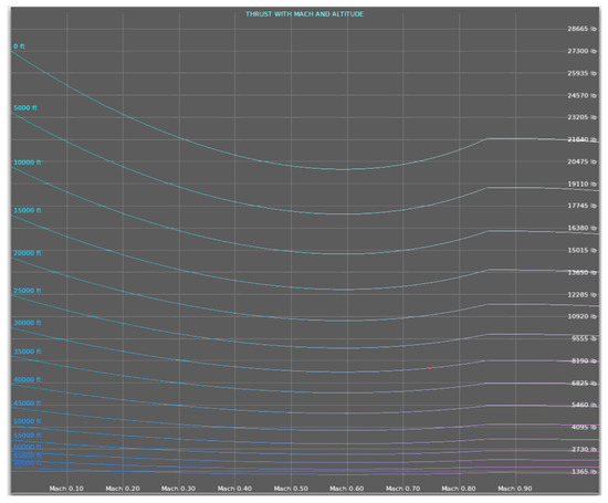
Figure 3.
CFM56-7B26 thrust production. Exported from the aircraft’s characteristics in the X-Plane 11 simulator.
In order to make use of the information in the diagram, the thrust that is in pounds has to be converted into Newtons, and the altitude to the corresponding air density. Taking into account that the X-Plane simulator uses the International Standard Atmosphere (ISA), the air density on the surface of the sea is exactly 1.225 kg/m3, with the temperature being at 15 °C and the pressure at 1013.25 hPa. The corresponding densities at the heights of 5000 ft, 10,000 ft, and 15,000 ft are 1.055 kg/m3, 0.904 kg/m3, and 0.771 kg/m3, respectively.
Only a certain range of data is extracted from the diagram of Figure 3, which contains the first four altitude lines of 0 ft, 5000 ft, 10,000 ft, and 15,000 ft, and velocities from 0 up to 0.3 Mach (198 Knots), with a step of 0.01 mach, with a total of 124 data points being collected. This certain range was selected because the calculations should be applicable to any airport in the world, with the highest being Daocheng Yading in China at an altitude of 14,471 ft, while the speed of 0.3 mach (198 Knots) is way greater than the V1 speed for this certain aircraft, in any possible configuration.
Based on these data and a polynomial fit, a function is generated that exports the thrust at any density and airspeed, within range. The following polynomial is used to fit the data to.
The selection of this quadratic function in two variables, with cross terms, is done for three reasons. Each altitude line can be described by a second degree polynomial. Additionally, the distance between each altitude line decreases as the height increases, which also signifies a second degree relation between the thrust and the altitude. Finally, the cross terms (those that contain both x and y variables), are used as they are necessary for an accurate fit of this complex correlation.
Subsequently, the selected velocities and densities construct the meshgrid A, containing 124 rows (all the combinations of 31 velocities in four different densities) and nine columns (as many as the terms of Equation (3)). Each row represents different combinations of x and y, i.e., velocities and densities.
Columns include the results of the variable-related part of the terms of Equation (3). The first column contains all ones, as there it is a non-variable related term. The second column contains only the x (velocity) related to that row. The eighth column contains the product of the row’s velocity multiplied by the square of the row’s density, and so forth.
Column B contains the samples of all 124 points of the diagram. The problem can be solved as a linear system, , in which x is the coefficients A,B,…I of Equation (3). The solution is calculated by solving through the least squares method. The Mean Absolute Error for the solution found is 7.005 Newtons.
The optical representation of the retrieved data and the fitted polynomial is depicted in Figure 4.
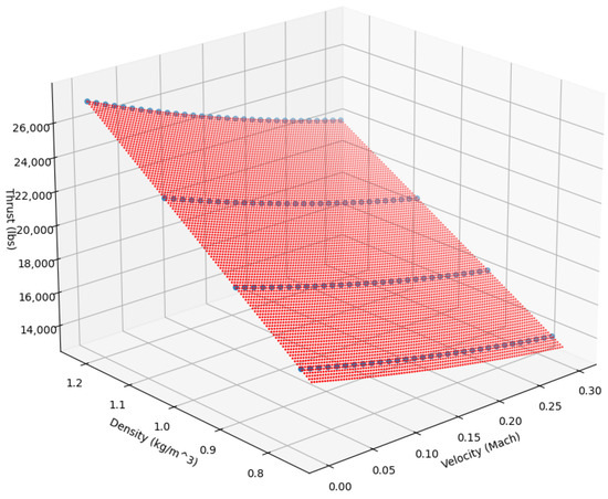
Figure 4.
Polynomial fit (red plane) and actual thrust data (blue dots).
Friction between the Runway and the Tires
When the aircraft is on the runway, the only points that interact with the runway are the tires, between which friction forces are being developed. They may be almost negligible during the acceleration, especially when comparing them with the thrust produced by the engines, but the aircraft’s braking system is the main stopping mean when decelerating. This makes its modeling vital.
The friction, , produced is calculated as the total force acting vertically on the tire, , multiplied by a friction coefficient, , as shown in Equation (4).
For simplicity reasons and as no significant deviation emerges from it, the force is considered to be a point force. Hence, based on Figure 2, the friction force is expressed as:
in which is the aerodynamic lift produced by the wings of the aircraft. The above equation makes the modeling of the produced by the wings mandatory.
Lift and Drag
The two forces produced by the interaction of the body with the surrounding air are the and . Calculated by similar equations, these can be expressed as:
in which:
- : aerodynamic lift;
- : aerodynamic drag;
- : lift coefficient;
- : drag coefficient;
- : air density;
- A: the projected area of the body vertical to the force;
- V: the airspeed of the aircraft.
It is well established that the lift and drag coefficients are heavily depended on the Angle of Attack (AoA), which is the angle difference between the airflow and the lateral axis that passes through the nose and the tail of the aircraft. Both lift and drag coefficients have typical curves, similar to these in Figure 5.

Figure 5.
Lift coefficient, CL, and drag coefficient, CD, of the NREL S809 airfoil [15].
While on the runway, the AoA is close to zero, with deviations of ±1.5 degrees as found through various tests in the simulator. Based on the typical curves, a strongly positive correlation is expected between the lift coefficient and the AoA, while on the other hand no correlation is expected between the drag correlation and the AoA.
The necessary code is developed that retrieves the lift and drag forces, the air density, and the velocity of the aircraft of each frame of the simulation, and calculates the coefficients through reverse engineering.
The crew of the aircraft has a set of flap settings to choose from. This aircraft’s set includes the settings notated as 0, 1, 5, 10, 15, 25, 30, 40. For each of these settings, flaps extend progressively more and achieve higher lift coefficients and therefore higher lift forces at the same speed. The counterbalance of these higher lift coefficients is also progressively higher drag coefficients for each of the settings. The five most common settings during takeoff and those modeled for the system are 1, 2, 5, 10, and 15. Similar methods can be used to model all the flap settings.
Weight Component
One of the characteristics of the runway is its slope. This is described as the height difference between the start and the end of the runway divided by its , and is expressed as a percentage (Equation (10)).
In order to transform the slope percentage to degrees (), the inverse tangent is used, as in Equation (11).
Given the angle , the gravitational force can be analyzed the in x- and y-axes, with one being perpendicular and the other being vertical to the aircraft’s axis of movement:
in which m is the total aircraft’s mass, g is the gravitational acceleration, and is the slope of the runway in degrees. Depending on the runway slope, either contributes or resists the achievement of a desired velocity, while is needed to calculate the total weight acting on the wheels.
3.1.2. Calculating Forces While Accelerating
There are two subsections about calculating the forces during a takeoff. Since the system aims to calculate the distance that will be covered by the aircraft in the case of a rejected takeoff (RTO) at speed V1, there are different calculations for the accelerating and the decelerating part of the procedure. The discrepancy between the two aims to the minimize the computations, and hence the time, needed to provide a result, without sacrificing its accuracy.
Engine Thrust
To calculate the thrust of the engines, a function is used to calculate the thrust based on density and airspeed. This output refers to the thrust produced by one engine at 100% N1, and is hence multiplied by two, which equals the number of engines.
Depending on the selected by the pilots’ N1 (primary thrust indicator), which may occasionally exceed 100%, the result has to be multiplied by the equivalent fraction. However, the relation between the N1 setting and the thrust produced is not linear, and hence the result cannot be multiplied by the N1’s percentage. The X-Plane simulator provides the mapping between the N1 and the produced thrust, which can be used to calculate the actual thrust in relation to the N1. For simplicity reasons and since this paper aims to prove the feasibility of such a system, it is considered that a constant N1 of 104% should be used. This N1 setting corresponds to 101.5% of the maximum thrust produced.
Additionally, the engines have a spoolup time that is needed to reach the desired maximum thrust. This time is calculated to be 7.5 s for this type of engine. The modeling of this transition utilizes a rational function with the general form of:
Then, the appropriate coefficients a,b,c,d,e,f are found, which describe the thrust for these 7.5 s as a fraction of the engine’s final thrust, in relation to the elapsed time (seconds), since the setting of the engine levers. The results of the actual and calculated spoolup thrusts are presented in Figure 6 and Figure 7. The mean difference is approximately 361 Newtons, which is negligible and not able to affect the final result.
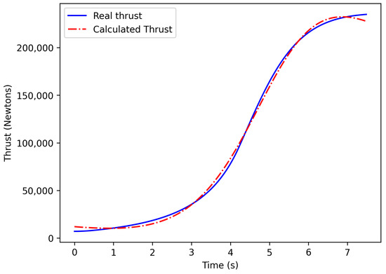
Figure 6.
Actual and calculated thrusts during spoolup.

Figure 7.
Difference between actual and calculated thrusts during spoolup.
Lift and Drag Coefficients, and Friction through Lift
The horizontal stabilizer is set based on the weight and the center of gravity of the aircraft. This provides aerodynamic stability around the lateral axis, both on the ground and in the air.
The abovementioned setting ensures that the AoA of the aircraft throughout the takeoff is around 0 degrees, with minor fluctuations of ±1 degree, as it is observed through testing. The lift coefficient faces big changes in this range. On the other hand, the friction force, which depends on the lift force, is multiplied by the rolling friction coefficient that is equal to or less than 0.025, on any runway condition, throughout acceleration. To this end, for simplification reasons and only for the accelerating part of the takeoff, it is concluded that a mean lift coefficient can be used for each of the flap settings. On the other hand, the drag coefficient faces little to no changes within this range, as seen through the typical graphs, and hence the mean value for each flap setting can also be used without heavily affecting the final result.
Weight Component
The weight component is calculated once, through the angle (as described before in Section 3.1.1), and is used as a steady force in the calculations.
3.1.3. Calculating Forces during Deceleration
Equally, if not more, important than the aircraft’s ability to attain speed is the ability to reduce it. As a structure that weighs between 52,000 kg and 78,000 kg [16], the aircraft is quipped with a number of means that can reduce the kinetic energy, those being brakes, spoilers, and thrust reversers.
The aircraft’s braking system works under the same principles as in cars, meaning that it transforms kinetic energy to thermal energy through friction. The overheating of the braking system leads to reduced performance and this is the reason that more than one stopping mean is mandatory for modern medium- and large-size aircraft. The second stopping mean is the wing’s spoiler. Placed on top of the wing, it differs from speedbrakes, as it not only increases the drag coefficient, but also disrupts lift production. Last are the thrust reversers, moving surfaces that divert the engine’s exhaust airflow, resulting in forces opposite to the aircraft’s moving direction.
The aircraft also has a number of options for the autobrakes, those being named RTO, 1, 2, 3, MAX. The last four selections concern the landing of the aircraft and aim to achieve certain deceleration rates. The RTO selection though is used in the case of a rejected takeoff and applies full pressure to the aircraft’s braking system, enabling the anti-skid system, until the full stop.
The calculation principle in the case of deceleration is common to that of the acceleration, meaning that the distance is calculated as a sum of parallelograms that derive from the acceleration’s double integral.
Engine Thrust
When decelerating, there are practically three modes for the engines to work in. The one is the idle thrust, in which the engine produces the minimum thrust pushing the plane forward, the reversers in idle thrust, which produce the minimum reverse thrust, and the reversers at the maximum setting. Apart from calculating the thrust produced in each setting as a fraction of the maximum produced thrust, the transitions to each one of the abovementioned states is also modeled using the rational function used to model the spoolup transition (Equation (13)). Indicatively, the modeled and actual transitions from full throttle to full reverse throttle can be seen in Figure 8.
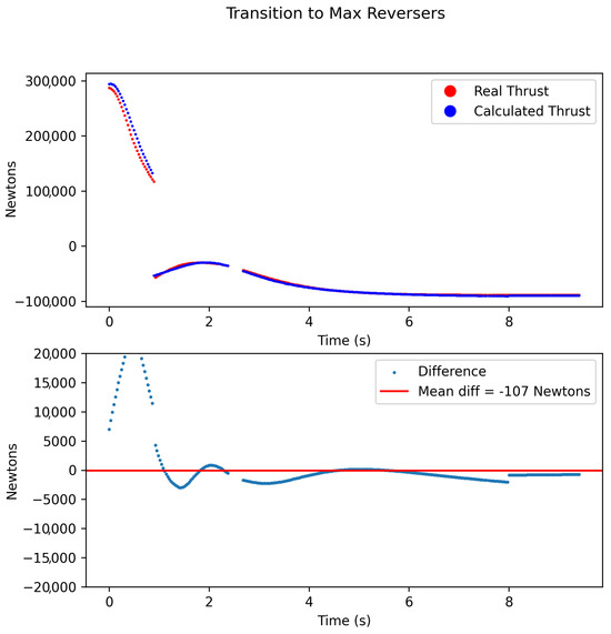
Figure 8.
Modeled transition to max reversers and actual transition.
Lift and Drag Coefficients
Throughout acceleration, the friction force is orders of magnitude smaller than those of deceleration. Using mean lift and drag coefficients in this case leads to fault propagation and inevitably to unrealistic deviations in terms of distance.
A more elaborate modeling of the lift and drag coefficients is performed by applying a least squares first degree polynomial fit to the collected data. In Figure 9, the data for flaps setting 1 are presented, along with the resulting fitted line. The linear behavior of the lift and drag coefficients in this range of Angle of Attack (AoA) is already established.
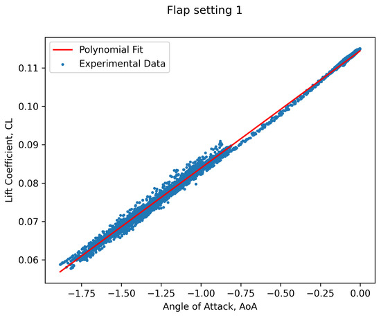
Figure 9.
Lift coefficient, CL, graph for flaps setting 1.
The lift coefficient for each of the flap settings can now be expressed through this general form equation:
In Figure 10, there are the fitted lines for all five of the modeled flap settings. It is clearly visible and expected that higher flap settings offer higher lift coefficients.
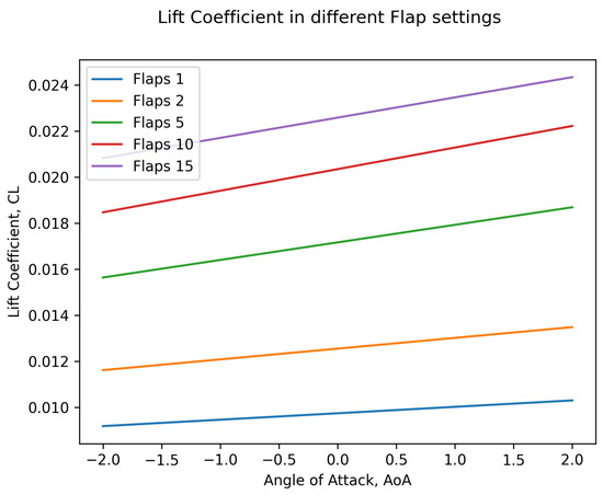
Figure 10.
Lift coefficients for each of the flap settings.
Each of the flap settings is also modeled with the spoilers deployed. Thus, any possible configuration can be predicted. The exact same process for both deployed and undeployed spoilers is used to model the drag coefficient in each one of the flap settings, as presented in Figure 11.
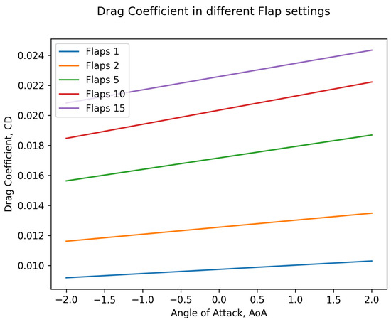
Figure 11.
Drag coefficients for each of the flap settings.
Angle of Attack
The modeling of AoA is now required in order to calculate the lift and drag coefficients. The factors affecting the AoA are divided in two categories, named primary and secondary. The primary factors include:
- Flap setting;
- Runway condition;
- Total aircraft weight;
- Ground Speed.
While the secondary factors include:
- Ambient temperature;
- Usage of speedbrakes;
- Thrust mode.
Regarding the primary set of factors, the first two are described by discrete values. The flap setting can be 1, 2, 5, 10, or 15, and the runway conditions can be dry, wet, or damp, as in the simulator. The last two though are described by continuous values. In order to model the AoA, the weight spectrum is sampled at seven values. Two of them are the minimum and maximum weight of the aircraft (51,860 kg and 79,091 kg). The range in between is sampled at 56,662 kg (5000 kg payload, 2 h normal cruise worth of fuel), 60,463 kg (7500 kg payload and two and a half hours autonomy), 64,495 kg (10,000 kg payload and 3 h of flight autonomy), 70,641 kg (15,000 kg payload and 3 h of fuel autonomy), and 75,826 kg (17,000 kg payload and 4 h of fuel autonomy). These weights are selected to represent possible flight configurations for short or longer range routes. The interval between each two weights is about 5000 kg, as it was noticed that there are no notable differences between smaller intervals.
Two runs are recorded for all the possible combinations between aircraft weight, flap setting, and runway condition. A common V1 speed of 70 m/s (136 knots) is selected among all runs on which the RTO is initiated, as all runs must contain similar data so they can be further analyzed. This speed is the minimum allowable speed among the configurations that will not lift the aircraft off the ground. During the deceleration, the speed and AoA are recorded. A total of 210 decelerations are executed in this experiment, for 105 different combinations of conditions.
Then, the processing procedure initially includes the fitting of the data for each couple of runs to a second degree function, using the least squares method. Figure 12 presents the data of AoA, as well as the fitted second degree function. The figure refers to a experimental configuration of 51,860 kg, flap setting 1, and a dry runway.
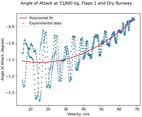
Figure 12.
Fitting of second degree function on the collected data for AoA and velocity. Experiment configuration 51,860 kg, flap setting 1, and a dry runway.
The following step includes the scaling of the modeling on the collected data. As previously mentioned, the primary factors of weight and velocity are continuous, and thus the same practice as in thrust calculation can be used. The data combination and results of flap setting 15 and a dry runway can be seen in Figure 13. More precisely, the blue lines represent the fitted second degree functions on the data of all seven different weight settings, run with a flap setting of 15 and on a dry runway. Then, these results are fitted to form a plane (seen in red dots), as in the thrust modeling. A total of 15 planes (for all possible combinations of five flap settings and three runway conditions) are constructed this way.
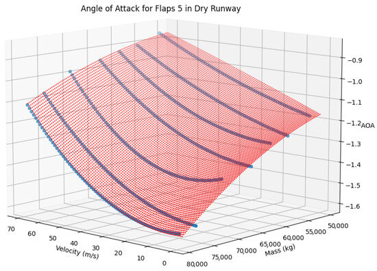
Figure 13.
Fitted plane of AoA on the continuous variables of velocity and weight. Results for flap setting 15 and a dry runway.
The secondary factors that affect the AoA are put in this category as they affect the whole plane equally on the vertical axis. Thus, a correction factor has to be added to the output of the corresponding plane. For example, negative temperatures affect the friction between the tires and the runway, as water and vapor turn into ice, which leads to reduced maximum braking capability and thus Angles of Attack closer to 0. Deployed spoilers are found to have the least affect on the AoA, but not at a negligible scale. The third and last secondary factor, which concerns the thrust mode (idle, reverse idle, and reverse max), is found to have quite a noticeable impact on the AoA while decelerating, but still only on the vertical axis.
A total of 36 correcting factors are calculated for each of the combinations between temperature (positive or negative), the three possible conditions of the runway, and the three possible thrust states. They are organized in two-dimension arrays and integrated into the AoA calculating function.
Tire Friction While Braking
The RTO setting of the autobrakes system applies full pressure to the pads, activating the anti-skid braking system of the aircraft. This leads to fluctuations in the actual friction force between the tires and the runway. The maximum force that can be applied before the tire starts skidding actually depends on two factors: the vertical force applied on the tires and the friction coefficient, . This coefficient describes the maximum ratio between the friction force, T, and the vertical force acting on the wheel, N, without loosing grip.
The friction coefficient, , depends on many factors, such as the type of the runway and its condition, the temperature, and the tire condition, pressure, and deformation. Since it is hard to determine tire-related factors in real world, the factors considered to affect the friction coefficient are the temperature (above or below 0 °C, the freezing point of water), and the runway condition (dry, damp, or wet). The only type of runway that commercial aircraft use are pavement runways, and thus this is the only type of runway examined.
The friction coefficient on pavement usually has values between 0.1 and 0.8 [17], depending on the condition of the runway and the ambient temperature. In order to take into consideration the anti-skid braking system of the aircraft, meaning the time intervals during which the pressure is released for the tire to roll and regain grip, the mean values of the coefficients are calculated.
More precisely, a plethora of tests are conducted in the whole range of available temperatures of the simulator (−24 °C–+52 °C), in all available runway conditions (dry, damp, and wet). We conclude that temperature only affects the friction coefficient depending on whether it higher or lower than 0 °C, which is the freezing point of water. Thus, it is expected to observe smaller friction coefficients at negative temperatures, as well as when the runway is wet.
The total combinations for the three runway conditions and the two temperature states (positive or negative) are six, as many as the output friction coefficients. They can be seen collectively in Figure 14. Hence, these are the friction coefficients that are used while braking in the RTO autobrakes setting, which takes into account the anti-skid braking system.
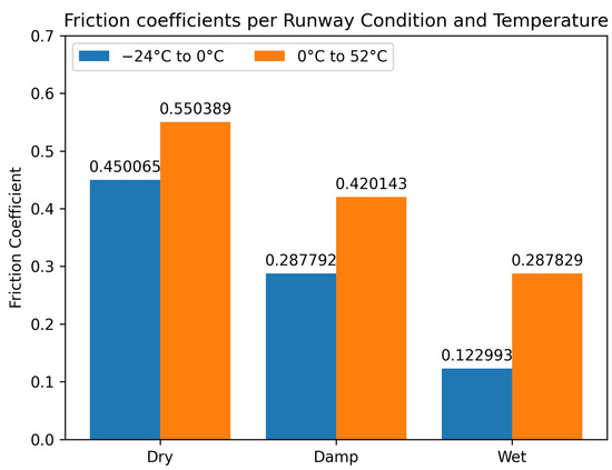
Figure 14.
Mean friction coefficients at different temperatures and in different runway conditions. Data from X-Plane 11 simulator, graph made by the authors.
Weight Component
The weight component is calculated once, through the angle (as described before in Section 3.1.1) and is used as a steady force for the calculations.
3.1.4. Additional Necessary Calculations/Conversions
Air Density
Air density plays a significant role in the aerodynamic calculations as well as the engine thrust. To calculate the air density, only two variables are necessary, those being the ambient temperature and the barometric pressure on the runway, named QFE.
The input variables are in degrees Celsius for the temperature and in hecto Pascals for the pressure. The way to convert them into air density is through the ideal gas law:
In which is the barometric pressure and RD = 287.05 Jkg−1K−1 is the gas constant for dry air.
Headwind Calculation and Boundary Layer
All takeoff and landing procedures are preferably and usually executed with a headwind instead of a tailwind for safety reasons, as this allows for greater air speeds in comparison with ground speeds.
To find the relation between the two speeds, the wind is analyzed in horizontal and vertical components to the runway axis. The only data needed are the heading of the wind and the heading of the runway. The forming angle between the two, noted as in Figure 15, is used to find the headwind component. In particular:
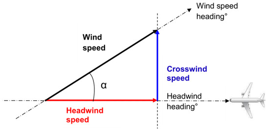
Figure 15.
Wind component analysis [18].
Then the wind speed can be multiplied by the cosine of , to find the headwind component:
The input and the output share the same measurement unit. Such data are available to the pilots via the control tower.
The boundary layer that is formed close to the ground, which reduces the speed of the air, has to be taken into account as well. Various tests with different wind speeds and directions unveil that the wind’s speed can be calculated if multiplied by coefficient . Hence, the headwind on the runway is expressed as:
Velocity Conversion
Avionics offers a variety of information including the Indicated Air Speed (IAS), the True Air Speed (TAS), and the Ground Speed (GS). The IAS is displayed in the primary flight display of the aircraft and is the speed that V1, VR, and V2 refer to, as well as VApp and VRef for the landing procedure. The conversion from IAS to GS is required to find the covered distance.
The different states followed to convert IAS to GS can be seen in Figure 16. The first step converts IAS to the Calibrated Air Speed (CAS). Systems onboard the aircraft add an error to the actual speed of the aircraft. A collection of values for both IAS and CAS indicates that the relation between the two is expressed as in Equation (20).
Figure 16.
Speed conversion states.
The Calibrated Air Speed refers to the speed in ISA (International Standard Atmosphere) conditions, which means that the ambient temperature and the barometric pressure are not taken into consideration. For given conditions of temperature and pressure, the air density can be found, and the conversion to True Air Speed is performed through Equation (21).
in which is the ISA conditions air density of 1.225 kg/m3, and is the actual air density.
The last step is to subtract the headwind from the TAS, as in Equation (22), in which all speeds refer to knots.
3.1.5. Overall Calculation of ASD Required
Since all the forces are modeled, it is possible to calculate the Accelerate Stop Distance Required (ASDR). The aggregate of inputs needed includes:
- The externally calculated V1 speed, in knots;
- Wind direction, in degrees;
- Wind speed, in knots;
- Ambient temperature, in degrees Celsius;
- Ambient Atmospheric Pressure on Elevation, QFE, in hPa;
- Flap setting;
- Total aircraft mass, in kg;
- Runway slope (as percentage);
- Runway condition
There is also the capability of calculating the distances when either using or not the spoilers, as well as when selecting different modes in engines during an RTO. When aborting a takeoff though, the pilots use all the braking means available, which means that they make use of the spoilers and the engines are set to the maximum reverse thrust. This is why these options do not necessarily have to be given as inputs.
Initially, the steady factors are calculated, those being the air density, the lift and drag coefficients during accelerating, the weight component, the headwind, and the friction coefficient while decelerating. Then, the algorithm executes the two while loops to calculate the acceleration and deceleration distances, with a top speed of V1, respectively. In each iteration of the two loops, the rest of the calculations (such as aerodynamic forces) are performed based on the current airspeed or Ground Speed of the aircraft.
As mentioned, the V1 speed is given by the user. A minor modification in the calculations and the additional input of the runway’s length, would allow for the calculation of the V1 speed by the system. In reality though, the majority of runways allow the attainment of the VR speed (speed at which the nose of the aircraft is lifted and the actual takeoff takes place), long before the aircraft is in danger of overrunning the runway. Additionally, the relations between the critical speeds of the aircraft are explicitly stated in EASA’s CS-25 file [9], and declare that the VR speed may not be less than the V1 speed.
In this condition, the strict definition of the V1 speed is abolished and the system is unable to calculate the correct speed. Furthermore, discrepancies between the system’s and other systems’ outputs (those that are exclusively made to calculate the critical speeds), would create confusion to the pilots, which should be avoided.
In addition to the previous calculations, a distance equivalent to two seconds at speed V1 is added on top of the previous result. This is considered to be the reaction time in case an engine failure happens at speed V1. It is an indivisible part of the Accelerate Stop Distance calculations, as CS-25 [9] states.
3.2. Dynamic Distance Calculations
Static calculations depend on many different factors and assume a smooth run in each process. However, one of the main and essential functions of the system is the prediction of distances in real time, in the event that the takeoff or landing of the aircraft does not run as predicted.
The dynamic calculations performed during takeoff are not based on any of the inputs mentioned in the static calculations. The only input they rely on is the acceleration (or deceleration) of the aircraft. In this context, it is necessary to analyze the data as well as the theory, to find a computationally efficient method capable of coping in real time, taking measurements of the acceleration at regular time intervals and performing the appropriate calculations.
3.2.1. Acceleration
Figure 17 shows a typical acceleration graph of a Boeing 737-100, which was modified and used by NASA (National Aeronautics and Space Administration). It is clearly visible that after spoolup (that usually lasts less than ten seconds, depending on the engine), there is a linear decrease in acceleration. This is because, as the speed increases, the produced thrust of the engines decreases and the aerodynamic resistance increases. At the same time, the friction between the wheels and the ground is reduced, but is the force with the least impact.

Figure 17.
Typical acceleration graph during a takeoff procedure. Boeing 737-100, modified by NASA [6].
After collecting data for the Boeing 737-800 on three random configurations, a corresponding graph was constructed. The expected linear relation after the spoolup is visible in all three configurations of Figure 18. More precisely, after the 7.5 s period that the engines need to reach full power, the acceleration rate decreases linearly with time.
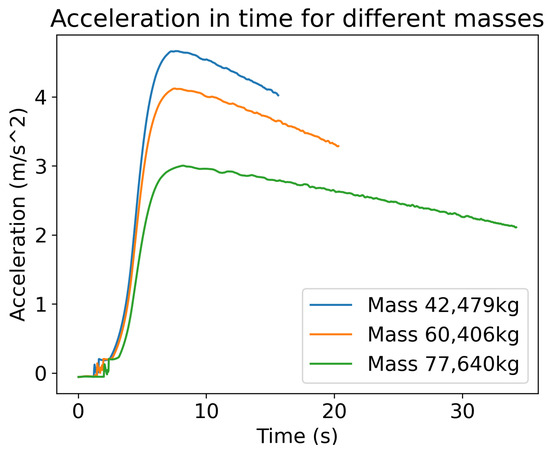
Figure 18.
Acceleration graph during a takeoff procedure in X-Plane 11, graph made by the authors. Boeing 737-800 in three different mass configurations.
Calculation of the Remaining Distance
To calculate the distance needed to achieve a certain velocity, we find the and coefficients that apply to the linear part of acceleration, when expressing it as one:
Then, by integrating Equation (23), the velocity equation derives:
where , are the same coefficients as in Equation (23), and is the already attained speed. Practically, it is the speed that the aircraft has achieved during the spoolup, right up to the start of the linear part. Since the speed that needs to be achieved is already known (speed V1), the time needed can be found by the solutions to this quadratic equation:
Taking into consideration Equation (25) and its coefficients, its discriminant is:
While the solutions are:
The coefficient always has a negative value, as the acceleration rate tends to decrease during the procedure, while the coefficient always has a positive value, representing the maximum achieved acceleration rate immediately after the completion of the spoolup. Hence, by projecting the accelerating function over time, the function will eventually be led to negative values. Then, the velocity starts to decrease due to the negative acceleration. This means that the solutions to the quadratic function, if any, will refer to the moments when V1 has been achieved, with positive acceleration values and negative acceleration values. The only real solution though is always the first of the two.
It is easily understood that there will always be solutions to satisfy the equation. No solutions would mean that the aircraft is not able to attain a speed equal to V1. In addition, the linearity of the acceleration function ceases to be in effect when it becomes close to 0, as the aircraft becomes closer to its terminal velocity.
Based on the above, the solution will always lie in the first of the two solutions. More precisely, based on Equation (27), the solution is:
Having found tV1 attainment, it is also possible to find the distance that is covered during this time as well. By integrating the velocity function, we obtain the distance function over time:
in which and are the coefficients from Equation (23), is the speed immediately after the completion of the spoolup, and is the distance already covered at t = 0. By replacing t with tV1 attainment, the distance is calculated.
Approximation of Acceleration and Factors
An equally important feature is the approximation of the and coefficients for the acceleration equation. Firstly, the nonlinear data of the spoolup’s 8 s (Figure 18) are not taken into consideration.
The next 3.5 s worth of data (time and acceleration) are used in a linear regression in order to determine the gradient of the function. The intercept is determined by the first collected value. These two values are used as seeds for the next algorithm.
Theoretically, all the samples that we obtain later than the 11th second can be saved in constantly increasing arrays and then processed by a linear regression algorithm. However, this solution is not efficient for a real-time system due to the exponential complexity of the algorithm. Instead, the Recursive Least Squares (RLS) filter is used, which uses the weighted least squares method to approximate coefficients and , without having to execute increasingly more calculations for every incoming measurement of acceleration. The RLS is used to approximate optimal coefficients of linear equations, structured like:
The algorithm also has an exponential complexity but the simplicity of the system, consisting of only two coefficients, keeps the total calculations at a consistent low number for each incoming data package. The linear equation that describes the acceleration over time can be also expressed as:
The RLS algorithm can be tuned through the forgetting factor, , which sets the significance of older samples. In this configuration, the forgetting factor is set to 1, as all the samples need to be of the same significance in order to output an accurate result and in order to converge faster.
3.2.2. Deceleration
The decelerating part of a rejected takeoff also has to be calculated dynamically. The RTO setting of the autobrakes though leads to fluctuating braking forces and thus fluctuating accelerations. The RLS filter can also be used to calculate the distance, but not with an identical structure. The alterations in measurements set the convergence to be impossible.
Calculation of the Remaining Distance
Due to the above reasons, the speed and the quadratic relationship approach that describes it are used instead of the acceleration. The quadratic equation that describes velocity over time is:
in which are the coefficients of the equation and t the time. Similarly, as before, the solutions to the quadratic equation can determine the moment in time at which the aircraft has zero velocity. The two solutions to the equation being zero, the final desirable speed and in correspondence to the coefficients of the previous equation are:
The deceleration rate during this procedure is not steady. The more the velocity drops, the more the lift force is reduced. This leads to greater vertical forces on the wheels, and thus the capability to apply more braking force before the tire starts skidding. Based on this observation, it can be determined that the coefficient of the velocity function will always be negative and will certainly be negative.
Based on the above ( being equal to to the speed of the aircraft), the equation has an inverted bell shape, whose maximum value lies above the horizontal axis. The graph meets the axis at two points, one ata negative t values and one at positive. The solution that is of interest to us is the latter one.
Since the signs of the and coefficients are both negative, the solution is found when subtracting the square root of the derivative:
Then, the ttill stop can be applied to the integral of the velocity function and the distance can be found. Thus, the distance is found through:
The constant term, , that results from the integral is equal to the distance that has been covered before the start of the dynamic calculations and after the initiation of the rejected takeoff.
Approximation of Velocity Coefficients
A rejected takeoff is considered to start when the throttle levers are pulled back. The duration of the pull back is approximately 0.8 s. During the next four seconds, many changes happen to the aircraft. The deployment of the spoilers and the spooldown of the engines affect the deceleration rate in nonlinear ways, and thus these four seconds of data are discarded. The next two seconds’ worth of velocity and time data are gathered and used in a least squares polynomial fit, in order to calculate the seeds of the last algorithm used. These seeds consist of three coefficients, , and , in correspondence to Equation (32).
Then, once again the Recursive Least Squares filter is used, with a slightly different configuration. The filter now tries to converge to three coefficients, instead of two, while the problem can be described as a linear equation like:
Once again, the forgetting factor, , is set to 1, as all the samples are of equal importance.
4. Landing Procedure
Landing is the most critical part of a flight and it includes a heavy workload by the pilots, as technical and aerodynamic configurations have to be taken into account, as well as the ambient conditions at the landing site. The accuracy and efficacy of the crew’s actions directly affect the passengers’ convenience and safety.
The most common type of accident during landing is the runway overrun [1], with causing factors including high approach and touchdown speeds, insufficient use of the reversers, etc. [19].
4.1. Velocities and Parts of Landing
Before the landing procedure starts, two critical velocities are calculated, those being VApp and VRef, based on a number of factors similar to those of takeoff. VApp is the speed at which the aircraft approaches the airport, while, for the final part, this speed is reduced down to VRef. This is practically the stall speed multiplied by a safety factor of 1.23, as CS-25 defines. This ensures a safe landing along with a minimum landing distance requirement.
The landing procedure can be divided into four stages: approach, flare, free roll, and braking, as Figure 19 indicates.

Figure 19.
Stages of landing.
The approach phase starts at the threshold of the runway at which supposedly the plane is at a height of 50 ft and a speed equivalent to VRef. The glide path followed may vary depending on limitations in the landscape around the runway, but it is 3 degrees (or less) for the vast majority of cases. Then, the flare phase starts at 20–30 ft above the runway, depending on the aircraft itself. This maneuver aims to reduce the vertical speed from ≈700 ft/min down to 60–180 ft/min, so that the aircraft can touch down smoothly. Elongated or early initiation of the maneuver can set the procedure in danger of a runway overrun, as the aircraft may be found hovering above the runway, wasting meaningful meters.
Immediately after touching the runway, the free roll stage begins. It lasts about 2 to 4 s, and aims to lower the nose of the aircraft, so that all wheels are in contact with the ground before applying any of the braking means. Last, but not least, the braking stage utilizes at least one of the decelerating means, till the aircraft comes to a full stop or it attains a taxiing speed of 20–30 knots. Since the system must be able to foresee an overrun, it calculates the distance needed to come to a full stop.
4.2. Static Calculations
The static calculations are performed after the user has given all the inputs needed to predict the total Landing Distance Required (LDR). Each part is estimated separately, in ways described in the following paragraphs.
All tests and modeling for the landing phase are executed using the autopilot function of the aircraft, on a Instrument Landing System (ILS) CAT-III equipped runway. In each part, there is a tendency for a slight overestimation (5–15%) by using mean-to-upper factors where applicable, as a safety measure, in case the system fails to estimate the LDR accurately.
4.2.1. Approach
The usual approach glide path for commercial aircraft stands at 3 degrees. Additionally, through simulations, it is concluded that the optimal height to initiate a flare for the Boeing 737-800 is at 30 ft. This means that the height difference between the two stages is 20 ft.
In Figure 20, the velocity component analysis for this specific glide path is shown, separating Vref into its vertical and horizontal components.
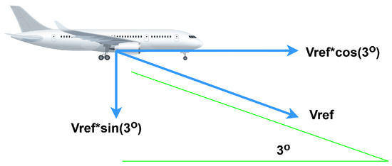
Figure 20.
Velocity component analysis on a 3 degree glide path during approach.
The time it takes for the aircraft from 50 ft to 30 ft is:
where refers to seconds and VRef is converted to feet per second. The distance covered during that time is:
where refers to feet and is converted to feet per second.
The overestimation alterations for this stage include the reduction of the theoretical glide path to 2.86° and the disposal of cos(3°) for calculating the horizontal speed. Thus:
4.2.2. Flare
Modeling the flare maneuver through a rational function is considered to be meaningless, since two flares may differ vastly. Instead, numerous tests are executed in order to find the mean values that describe the outcome of the process. It is concluded that a flare lasts 4 to 8 s, with a tendency towards the lower limit. For the static calculations, it is considered to last 5.5 s, slightly more than the average time. The average velocity maintained during the flare is found to be 2.1% less that Vref. Hence, the distance covered during the flare is:
where DFlare and VRef are in feet and feet per second, respectively.
4.2.3. Free Roll
Through similar processes, it is concluded that there is an average loss of 7.5% off the Vref speed at the moment that the aircraft touches the ground, and it is considered to remain steady for the duration of this phase. Free roll lasts for 2 to 4 s, with the mean-to-upper value of 3.5 s being used for the static calculation. The free roll distance calculation is:
where DFree Roll and VRef are in feet and feet per second, respectively.
4.2.4. Braking
For the fourth and last part of landing, the pilots have the option to either use the braking system manually or use the autobrakes in one of the four available settings, 1, 2, 3, or MAX. The static calculations have to be done based on an expected behavior, so there is an input for the landing procedure with these settings available.
Each one of them achieves a certain deceleration rate during the braking stage, ranging from 1.2 m/s2 to 4.1 m/s2 [20]. Additionally, ranging temperatures have a minor impact on this rate, while thrust reversers add 0.05 m/s2 to 0.22 m/s2 to this rate.
Based on the expected deceleration rate, the braking distance is found. Velocity while braking can be expressed though this time function:
in which is the velocity over time t, is the velocity at t = 0, at which braking started, and acceleration is the expected acceleration rate.
Setting the final desired speed to 0 and solving for t, we obtain the time needed till the aircraft stops, :
By integrating the velocity function and replacing t with Ttill stop, we obtain the distance covered while braking, :
4.3. Dynamic Calculations
As in the takeoff procedure, dynamic algorithms are also developed for the landing procedure.
4.3.1. Pre-Approach
As EASA’s Certification Specifications describe, a ROAAS system must be able to inform the crew for a longitudinal excursion in flight (from a given height) and on the ground. For this reason, an extra stage named Pre-Approach is added to the dynamic calculations, starting at 330 feet above the runway level and ending at 50 ft.
The system in this stage saves the last 100 values of the vertical and horizontal speeds and calculates the moving average of both of them. The sensitivity of the system can be tuned by changing the number of the last values kept. Based on the data output rate of that the simulator produces, this setup leads to a moderate sensitivity (about 30 samples per second). Embedding the system to a real aircraft, would require tuning in regard to the data output rate to the aircraft’s avionics.
Based on the average vertical speed and the current altitude, the time needed to reach 50 ft is calculated. This time is multiplied by the average horizontal speed to find the distance that is covered for the aircraft to reach 50 ft of altitude above the runway.
4.3.2. Approach
Similarly, the moving average of both horizontal and vertical speeds is calculated, but for this part the algorithm is more sensitive, keeping the 80 last samples. The new threshold is now 30 ft above the ground, which is where the flare stage starts. Other than that, the calculations for the distance prediction are identical.
4.3.3. Flare
As previously mentioned, the flare maneuver cannot be modeled or predicted, and thus the same configuration is used with an even higher sensitivity, keeping only 50 of the last values. The threshold for the last airborne part of the landing is 0 ft. The calculations are identical to those of the previous two parts.
4.3.4. Free Roll
Immediately after touching down, the free roll stage starts. For the static and dynamic calculations, a duration of 3.5 s is considered.
Initially, the start time is saved to a variable, while the moving average of the last 40 values of horizontal speed in feet per second is calculated.
For every new sample, the past time from the start of the free roll is calculated:
Then, the time left to the 3.5 s of the considered duration is computed:
Using the moving average of the horizontal speed, the distance left till the end of the free roll is determined:
In case the braking distance is not initiated before the end of the 3.5 s, then the time left is considered to be 0.5 s and the distance left is given by:
The reaction time of 0.5 s is selected because it sets an additional safety distance in the calculations and thereby gives time for the pilots to initiate the braking. At the same time, it does not trigger the system unintentionally with an excessive overestimation.
4.3.5. Braking
The last part of landing, braking, is triggered when pressure is applied to the brakes either by the autobrake system or by the pilots. The values of initial time and velocity are saved for further use.
Again, the Recursive Least Squares algorithm is utilized, as in the deceleration of the aircraft during a rejected takeoff. The algorithm aims to minimize the sum of the squares of the difference between the approximated and the actual coefficients that describe the velocity as a second degree function:
The difference is that the deceleration in this case is overall steady with minor fluctuations. The seed value in this case is 0.005 for coefficient , the anticipated deceleration rate for , and the initial velocity at the start of deceleration for .
The reason for using an coefficient different from 0, as would be expected for a steady deceleration, lies in the way that the remaining distance is calculated. As a second degree function, the time at which the speed is eliminated can be found through the discriminant:
And the actual time:
By integrating the velocity function (Equation (50)) and using the time found through Equation (52), the distance needed till the aircraft comes to a full stop can be found:
The constant of integration that arises from the integral is practically zero, because the dynamic algorithm of this state starts after the initiation of braking.
4.3.6. Dynamic Calculation of LDR While Landing
The principle behind dynamically calculating the LDR is that the remaining distance for the current stage is calculated in real time and the static estimations for the rest of the process are summed to output a single result.
In Table 1, the current stage is presented in each line of the table, while the type of result (statically calculated or dynamically calculated) used in the sum is presented in the columns of the table.

Table 1.
Usage of statically and dynamically calculated results during the landing procedure.
The dynamic result has meaning only when compared with the position of the aircraft relative to the runway. For this reason, a data structure is made, including the coordinates of the thresholds of all runways, based on the simulator’s data. The input given by the user includes the ICAO code of the airport and the runway marking. The returned data are the elevation of the runway, its length, and the threshold’s geographical location. Equivalent aeronautical data, such as the FAA’s National Airspace System Resource (NASR) System [21], can be utilized for a real-world application.
Having the threshold’s and the aircraft’s geographical data, through the GPS system, their relative distance is calculated through the Haversine algorithm.
Let the absolute distance of the aircraft from the runway be and let the distance from the previous calculation be , we can find whether the aircraft has passed the threshold. If the sign of the subtraction is positive, this means that the newly calculated distance is smaller than the previous one, and thus the aircraft is still approaching the threshold. In the occasion that the sign is negative, then the aircraft is above the runway.
Let the be the dynamically calculated Landing Distance Required. If the aircraft has not passed the threshold, then:
If the aircraft is past the threshold, then:
Finally, since the length of the runway is already known, the comparison between the LDR and the length can determine whether the aircraft is in danger of overrunning the runway.
5. Performance Evaluation
The performance evaluation of a safety system is a crucial part of its development. This is why numerous tests have been designed and executed for the majority of the input parameters that a user can input into the system.
The only parameter that has not been taken into consideration, even though the system fully supports its input, is the runway gradient. This is for two reasons.
Firstly, the simulator has the option to either render the runway as a completely flat surface or add the gradient based on the surface characteristics. The latter creates unrealistic runway gradients, with steep bumps that often cause the aircraft to bounce on them. This creates misleading scenarios and the data collected from such runs are not of any use. This is why the former option was selected.
The second reason is that, even if a slope is rendered to be as realistic as possible, the gradient of a runway is calculated as the height difference between the two thresholds. Any height differences in between are practically not taken into consideration. This is an already discovered problem with such systems [22], while the best promising method would be to collect analytical data for the elevation across the runways.
The modeFRONTIER automation and design software [23] is used to design the experiments. More precisely, the software has a Design of Experiments (DoE) mode, in which all the independent parameters, their range, and the total desired number of experiments are entered. A set of experiments is exported based on a quasi random Sobol sequence, exploring the widest possible range of combinations.
A total of 200 experiments are designed for each procedure (takeoff and landing) and the corresponding data are collected and used to reproduce the results that the system would output, in both static and dynamic modes.
5.1. Takeoff Performance Evaluation
All the experimental runs consist of rejected takeoffs exactly at speed V1. The variables and the corresponding value range (or available options) can be seen in Table 2.
Table 2.
Variables and their ranges used in takeoff design of experiment.
Velocity V1 is practically a dependent variable, and thus a simplified equation is constructed to calculate the appropriate velocity for each of the runs. This equation is:
This simplified equation outputs a range of ’s from 112 knots to 138 knots depending solely on the weight of the aircraft. This aims to approximate the real V1 speed without coming close to the speed at which the plane would become airborne.
5.1.1. Static Takeoff Calculation Performance
The static calculations that the comparison is performed with do not include the 2 s at the V1 distance, which EASA’s regulations set as a reaction time and safety parameter. This aims to show the exact difference between the static and the dynamic calculations, without taking into consideration the human factor.
Three comparisons are performed to determine the accuracy of the system. The first is about the acceleration distance, seen in Figure 21. For each of the runs, the percentile deviation is calculated, while the results are presented in a histogram, along with the standard deviation and the mean value of these results. It is found that the average difference is −0.18%, with a standard deviation of 0.55%. This means that, for 95.5% of occasions, the difference is [−1.28%, +0.92%].
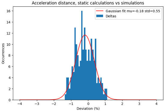
Figure 21.
Deviation of statically calculated acceleration distance and actual acceleration distance.
Similarly, regarding the deceleration distance, seen in Figure 22, the mean difference is +0.07%, with a standard deviation of 1.15%, due to the higher complexity of the calculations executed.

Figure 22.
Deviation of statically calculated deceleration distance and acceleration distance of the simulation.
Cumulatively, the ASDR distance is slightly underestimated by 0.02%, with a standard deviation of 0.73%, as Figure 23 indicates. This means that, for 99.7% of times, the static calculations differ by a percentage within [−2.21%, 2.17%].
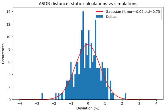
Figure 23.
Deviation of statically calculated ASDR and actual ASDR.
5.1.2. Dynamic Takeoff Calculation Performance
The performance of the dynamic calculations is evaluated in two ways, namely the time needed by the algorithm to converge and the deviation of the last prediction.
As seen in Figure 24, the first predictions of the algorithm, at 11 s, that derives from the seeds underestimates the distance needed to achieve V1. Half a second later, the mean prediction is at +2%, and 12 s after the initiation, the mean prediction is at +1%. It comes though with a high standard deviation (light-blue background that equals ), which sets the result to be non-utilizable.
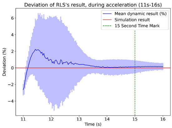
Figure 24.
Deviation of the RLS algorithm’s dynamic results from 11 s to 16 s since the takeoff’s initiation.
Instead, the 15 s time mark is set as the time after which the RLS’s mean result is close enough to a 0% deviation and the standard deviation is around 1%, with a tendency to decrease even more over time. Thus, the algorithm converges and the result can be safely compared with the statically calculated one.
Throughout the 200 runs, the last prediction of the dynamic algorithm has a mean difference of +0.29% when compared with the actual result, with a standard deviation of 0.26%. The histogram can be seen in Figure 25.

Figure 25.
Histogram and normal distribution of the RLS’s last prediction, before achieving velocity V1.
A similar evaluation is also performed for the decelerating part. In Figure 26, the mean estimation over time can be seen. At about 6.8 s after the initiation of a rejected takeoff, the first dynamic result is available. Initially, there is an underestimation of about 10%, but this changes rapidly. The mean overestimation peaks at about 2.5%, 8.5 s after the initiation, and then continuously converges to a 0% deviation.
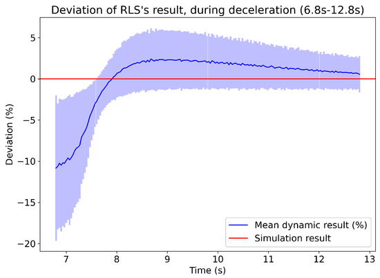
Figure 26.
Deviation of the RLS algorithm’s dynamic results from 6.8 s to 12.8 s since the beginning of an RTO (initiation of thrust reduction).
Since there is no heavy overestimation that can falsely trigger the system with a warning, there is not a time mark equivalent to the previous procedure’s. All the dynamic results produced by the RLS are treated equally and they are compared with the statically calculated ASDR, which also includes a distance equal to two seconds at speed V1.
The algorithm’s last prediction can be seen in Figure 27. The mean deviation stands at −0.02%, while the standard deviation is 1.28%. This proves that, up to the end of the deceleration, the algorithm converges realistically close to the actual distance. The outlier standing at −9% derives from an experiment with a strong tailwind (21 knots), a scenario that could not have occurred in an actual takeoff procedure.
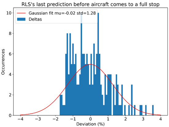
Figure 27.
Histogram and normal distribution of the RLS’s last prediction before the aircraft comes to a full stop.
5.2. Landing Performance Evaluation
Another 200 experiments are designed for the landing process through the same DOE generating software.
In Table 3, the corresponding variables and their ranges (or available options) can be seen. The maximum weight is adjusted to the maximum landing weight suggested by the manufacturer [16]. The settings for flaps used during landing are 30 and 40, and the autobrakes can be set at settings 1, 2, 3, or MAX, and so it is in the experiments.
Table 3.
Variables and their ranges used in landing’s design of experiment.
The output file is adjusted in certain ways. Specifically, all experiments that are executed with a tailwind greater than 10 knots are manipulated in their wind direction or wind speed. Landings with tailwinds are also avoided in real-world operations, for they enhance the danger of a runway excursion.
The Vref speed is calculated through a simplified algorithm, presented in Equation (57). It outputs a range of 129 to 143 knots in flap setting 40, and 136 to 150 knots in flap setting 30, based solely on the aircraft’s weight. This provides a rough approximation of the Vref speeds used in real-world procedures. Nevertheless, the output speeds are greater than the Vs0 (stall) speed in all cases.
5.2.1. Static Landing Calculation Performance
The results for the comparison between the static calculations and the actual distances per stage of landing, and for the total Landing Distance Required can be seen in Figure 28. All stages and the overall distance are slightly overestimated, except for the flare and free roll distances. Their mean deviation is around 25–30%, while they also have much larger standard deviations.
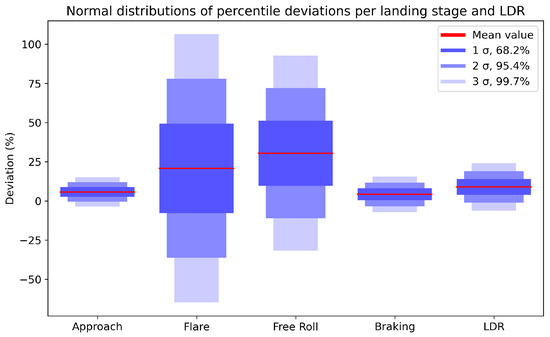
Figure 28.
Normal distribution of deviations per landing stage and for the total Landing Distance Required.
These data may at first sight be an issue for the performance of the system. However, as previously mentioned, flare is a hard to model and almost impossible to predict maneuver. An analysis between this stage and the free roll, which also has an even greater mean value, is conducted to reveal more insights about the two stages. Executing a linear regression between the data and visualizing it, as in Figure 29, it is obvious that there is a negative correlation between the deviations of the two stages. This means that the bigger the deviation is at the flare stage, the smaller it is in the next stage, that of the free roll, and vice versa.

Figure 29.
Correlation between the flare stage and the free roll stage of landing.
Finally, a more detailed look in the results of the statically calculated LDR distance reveals an average overestimation of 8.98% and a standard deviation of 5.05%. These results can be seen in Figure 30.
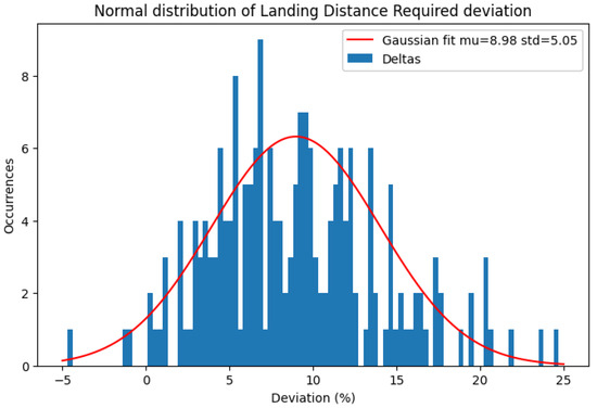
Figure 30.
Normal distribution of statically calculated Landing Distance Required and actual result.
As depicted in the diagram, there are instances where the overall LDR distance is underestimated (deviation < 0). However, upon individual examination of these instances, it becomes apparent that the disparity arises from the flare stage, which is underestimated by an average of 27% (Table 4).
Table 4.
Detailed results of landing experiments with a negative deviation.
Similarly, corresponding results arise from the examination of cases where the estimation exceeds the actual result by at least 20%. Most of the overestimation stems from the horizontal component (Table 5, study of three of the cases).
Table 5.
Detailed results of three of the landing experiments with a positive deviation.
5.2.2. Dynamic Landing Calculation Performance
The performance of most of the landing procedure’s dynamic stages cannot be represented collectively, due to the lack of a common basis for the data to be presented within. A common basis that could be used is time, but the varying and usually short duration of the stages sets a comparison devoid of revealing useful and insightful information.
The part that could be analyzed though, due to its greater duration, is that of braking, which utilizes the RLS algorithm. From the moment braking is initiated, the RLS is able to produce results, due to the almost complete absence of slope in the deceleration rate. Therefore, after processing the data from the 200 experiments, the average values and variances during the first 8 s of braking are obtained. As shown in Figure 31, initially there is a negative deviation in the result of approximately −7.5%. This changes at 4 s, reaching a maximum later, at 5.2%. From there on, the algorithm converges to 0%, with the prediction at 8 s having an average value of 0.13% and a standard deviation of 2.4%.
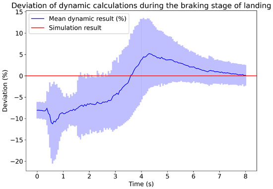
Figure 31.
Mean and standard deviation of landing procedure’s dynamic braking calculations.
6. Conclusions
The aim of the system is to predict runway overruns in real time for both takeoff and landing procedures. Two types of algorithms are developed, including static and dynamic calculations of the remaining distance needed by the aircraft to come to a stop. The algorithms are developed frugally in order to minimize complexity, without compromising in terms of accuracy. Additionally, the vast majority of affecting factors are taken into consideration in the widest range possible, so that the system is able to perform in any probable scenario with the same reliability.
All the system’s inputs are carefully selected, such that they are either available to the pilots or accessible through the aircraft’s avionics system. This results in a less complex embedding process, along with the reliability of the already developed systems and processes.
The results of the evaluation process provide sufficient evidence that the algorithms can be used in a real-time overrun avoiding system. Both procedures, takeoff and landing, can be predicted with adequate accuracy statically, while the dynamic algorithms are able to predict the distance needed based solely on the development of the process. Their comparison can provide a reliable result, evaluating the danger of an overrun, in the case that the takeoff or landing procedure is continued as is.
The results of the takeoff procedure indicate that a system that integrates static and dynamic calculations to assess the ASDR is feasible, which is a significant advance when compared with the existing TOPMS. The performance of the corresponding systems for the landing procedure (RAAS and ROPS) are not publicly available due to the proprietary nature of the data and their sensitivity within airline safety operations. The RUNSAFE system, though, offers unification of the takeoff and landing procedures, leading to a consolidated runway overrun prevention system. This enhances safety by providing a consistent operational interface, ensuring more reliable and straightforward decision-making during these critical flight phases.
The algorithms have also been embedded to a RaspberryPi 3b, with a 7 inch touch display and speakers for interaction purposes, to form a prototype system. The Raspbian operating system is used, while the application is developed through the Qt application development framework. All the algorithms are developed in C++, due to adaptability and performance reasons. The application has two modes, one for takeoff and one for landing, with the corresponding configuration screens. The procedure screen of both modes has a common structure, and the system displays and announces messages depending on the real-time result [24].
Future visions of the system include the adoption of the aircraft’s center of gravity in the static calculations, so that all factors are taken into consideration when calculating the Accelerate Stop Distance Required and the Landing Distance Required. Furthermore, it is vital that the system is also evaluated for the runway’s slope, an unweighted factor for reasons described in previous sections.
Another considered approach is to reproduce real runway overrun events, in order to assess whether the system and algorithms would be able to notify the pilots in sufficient time an the accident to be prevented.
Author Contributions
Conceptualization, G.A., I.K., A.K. and A.P.; methodology, G.A., I.K., A.K. and A.P.; software, G.A.; validation, G.A., I.K. and A.K.; writing—original draft preparation, G.A.; writing—review and editing, G.A., I.K., A.K. and A.P.; visualization, G.A.; supervision, V.K. All authors have read and agreed to the published version of the manuscript.
Funding
This research received no external funding.
Data Availability Statement
Dataset available on request from the authors.
Conflicts of Interest
The authors declare no conflicts of interest.
Abbreviations
| RUNSAFE | Runway Safety Assistant Foreseeing Excursions |
| ASD | Accelerate Stop Distance |
| ASDR | Accelerate Stop Distance Required |
| LDR | Landing Distance Required |
| ISA | International Standard Atmosphere |
| RTO | Rejected takeoff |
| AoA | Angle of Attack |
| QFE | Pressure at Field Elevation |
| IAS | Indicated Air Speed |
| TAS | True Air Speed |
| GS | Ground Speed |
| CAS | Calibrated Air Speed |
| NASA | National Aeronautics and Space Administration |
| EASA | European Aviation Safety Agency |
| FMS | Flight Management System |
| ROAAS | Runway Overrun Awareness and Alerting Systems |
| ROPS | Runway Overrun Prevention System |
| RAAS | Runway Awareness and Advisory System |
| TOPMS | Takeoff Performance Monitoring System |
| TOPAP | Takeoff Performance Alerting Program |
| IATA | International Air Transport Association |
| RLS | Recursive Least Squares algorithm |
Appendix A
The following datarefs were used from the X-Plane 11 simulator, during the development and validation of the system.
Table A1.
Datarefs used from the X-Plane 11 simulator.
Table A1.
Datarefs used from the X-Plane 11 simulator.
| Field Num. | Field Name | Field Description |
|---|---|---|
| 1 | Time | Time since last reset (seconds) |
| 3 | Ground Speed | Ground Speed (knots) |
| 3 | IAS | Indicated Air Speed (knots) |
| 3 | EAS | Equivalent Air Speed (knots) |
| 3 | TAS | True Air Speed (knots) |
| 4 | Speed | Speed (Mach) |
| 4 | VSI | Vertical speed indicator (ft/min) |
| 4 | Acceleration | Longitudinal acceleration (g) |
| 14 | Brakes | Brake usage (ratio 0–1) |
| 18 | AoA | AoA (degrees) |
| 20 | Longitude | Geographic coordinates (degrees) |
| 20 | Latitude | Geographic coordinates (degrees) |
| 21 | Distance | Distance covered since last reset (ft) |
| 25 | Throttle | Throttle usage ratio (0–1) |
| 35 | Thrust | Thrust produced by engines (lbs) |
| 64 | Lift | Total lift produced (lbs) |
| 64 | Drag | Total drag produced (lbs) |
| 137 | Friction force | Friction force with runway (lbs) |
References
- IATA. Runway Safety Accident Analysis Report; Technical Report; IATA: Montreal, QC, Canada, 2015. [Google Scholar]
- Kharoufah, H.; Murray, J.; Baxter, G.; Wild, G. A review of human factors causations in commercial air transport accidents and incidents: From to 2000–2016. Prog. Aerosp. Sci. 2018, 99, 1–13. [Google Scholar] [CrossRef]
- NAVBLUE. Flysmart+. Available online: www.navblue.aero/product/flysmart-plus/ (accessed on 28 July 2024).
- EASA. EASA Publishes Research Agenda 2022–2024; EASA: Cologne, Germany, 2022. [Google Scholar]
- SAE. AS8044A: Takeoff Performance Monitor (TOPM) System, Airplane, Minimum Performance Standard; SAE International: London, UK, 2020. [Google Scholar]
- Middleton, D.B.; Srivatsan, R.; Person, L.H., Jr. Flight Test of Takeoff Performance Monitoring System; Technical Report; National Aeronautics and Space Administration: Washington, DC, USA, 1994. [Google Scholar]
- EASA. Annual Safety Recommendations Review 2018; EASA: Cologne, Germany, 2018. [Google Scholar]
- Benard, B.; Nijhof, M.; Van Es, G. Take-Off performance incidents: Do we need to accept them or can we avoid them? In Proceedings of the ISASI Annual Seminar, Hague, The Netherlands, 1–6 September 2019.
- EASA. CS-25 Amendment 27—Review of Aeroplane Performance Requirements for Air Operations and Regular update of CS-25; EASA: Cologne, Germany, 2023. [Google Scholar]
- Heidt, A.; Helmke, H.; Kapolke, M.; Liers, F.; Martin, A. Robust runway scheduling under uncertain conditions. J. Air Transp. Manag. 2016, 56, 28–37. [Google Scholar] [CrossRef]
- Wagner, D.C.; Barker, K. Statistical methods for modeling the risk of runway excursions. J. Risk Res. 2014, 17, 885–901. [Google Scholar] [CrossRef]
- Gao, P.; Sun, Y.; Zhou, X.; Zhang, Y. Construction of Safety Constraint Model Based on STPA and Improved AHP for Runway Excursions. In Proceedings of the 2023 IEEE 5th International Conference on Civil Aviation Safety and Information Technology (ICCASIT), Dali, China, 11–13 October 2023; pp. 464–470. [Google Scholar]
- Melvin, W. Certification and application of rejected takeoff procedures. In Aircraft Design, Systems, and Operations Meeting; American Institute of Aeronautics and Astronautics: Reston, VA, USA, 2012. [Google Scholar] [CrossRef]
- Gudmundsson, S. General Aviation Aircraft Design: Applied Methods and Procedures, 2nd ed.; Butterworth-Heinemann: Oxford, UK; Cambridge, MA, USA, 2022. [Google Scholar]
- Spera, D. Models of Lift and Drag Coeffi cients of Stalled and Unstalled Airfoils in Wind Turbines and Wind Tunnels; NASA: Washington, DC, USA, 2008. [Google Scholar]
- Boeing Commercial Airplanes Company. 737 Airplane Characteristics for Airport Planning; Boeing Commercial Airplanes: Seattle, WA, USA, 2005. [Google Scholar]
- Novikov, A.; Novikov, I.; Shevtsova, A. Study of the impact of type and condition of the road surface on parameters of signalized intersection. Transp. Res. Procedia 2018, 36, 548–555. [Google Scholar] [CrossRef]
- IVAO. Crosswind and Headwind Calculation. Available online: https://wiki.ivao.aero/en/home/training/documentation/Crosswind_and_Headwind_calculation (accessed on 28 July 2024).
- Jenkins, M.; Aaron, R. Reducing Runway Landing Overruns. Aero Mag. 2012, 3, 14–19. [Google Scholar]
- Flaps2Approach. B737 Auto Brakes–Converting & Using a Genuine Auto Brake. Available online: www.flaps2approach.com/journal/2013/3/18/b737-auto-brakes-converting-using-a-genuine-auto-brake.html (accessed on 28 July 2024).
- FAA. 28 Day NASR Subscription. Available online: www.faa.gov/air_traffic/flight_info/aeronav/aero_data/NASR_Subscription/ (accessed on 28 July 2024).
- Foxworth, T.; Marthinsen, H. Another look at accelerate-stop criteria. In Proceedings of the AIAA Aircraft Design and Operations Meeting, Los Angeles, CA, USA, 14–16 July 1969; p. 772. [Google Scholar]
- modeFRONTIER. Simulation Automation and Design Optimization. Available online: https://engineering.esteco.com/modefrontier/ (accessed on 28 July 2024).
- Alogdianakis, G.; Katsidimas, I.; Kotzakolios, A.; Plioutsias, A.; Kostopoulos, V. An Embedded Decision Support System for Runway Safety and Excursion Avoidance. arXiv 2024, arXiv:2407.02504. [Google Scholar]

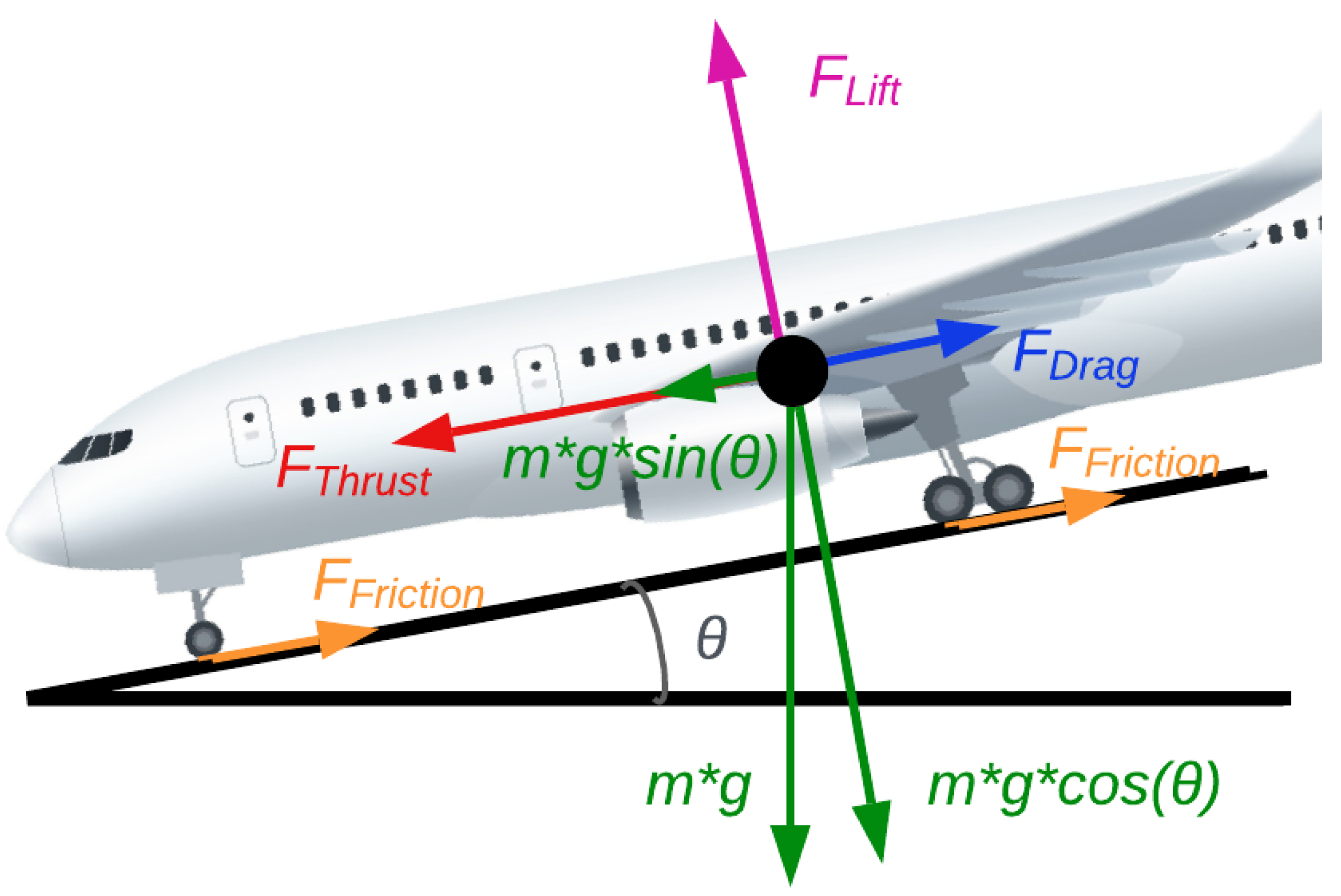
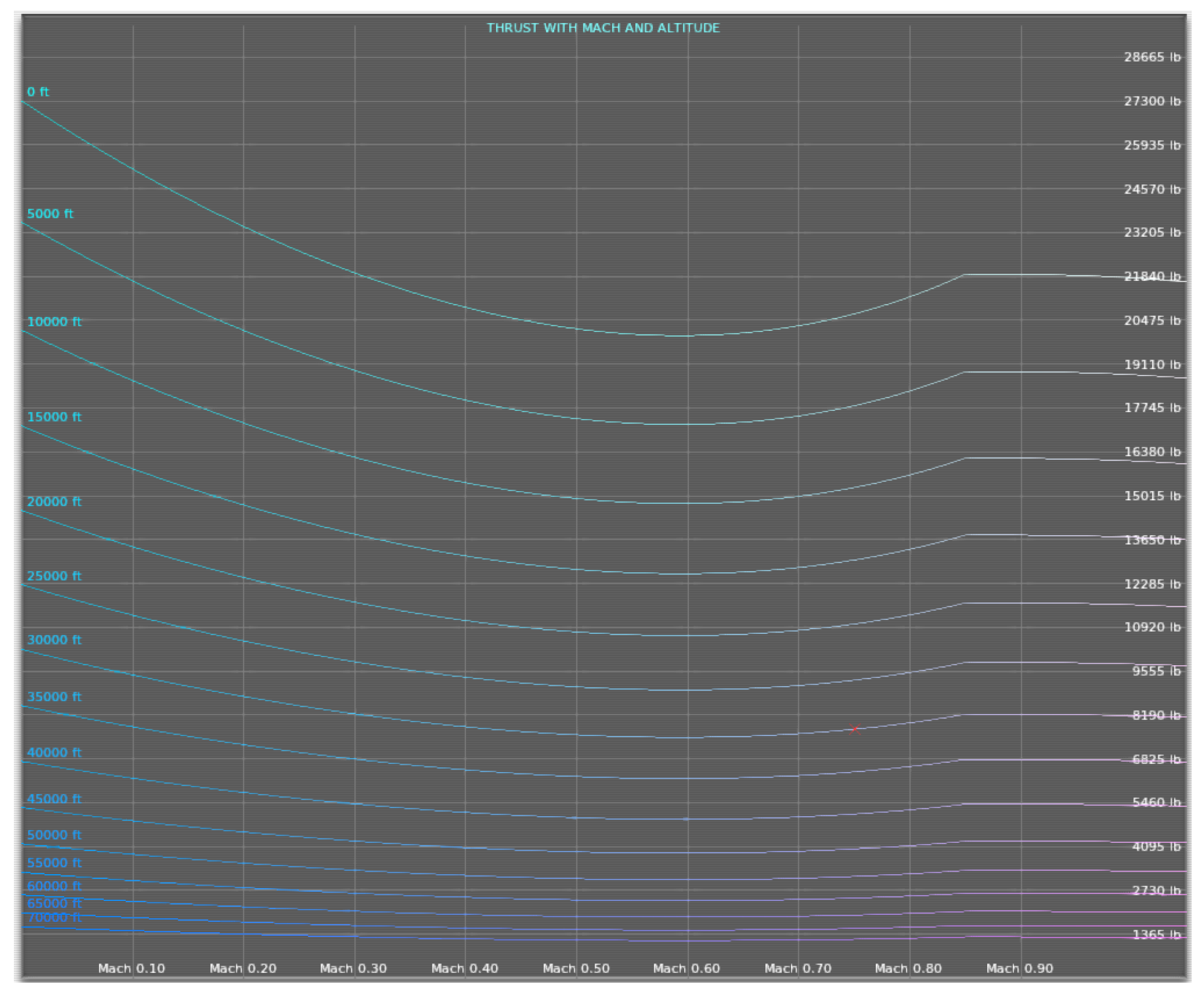

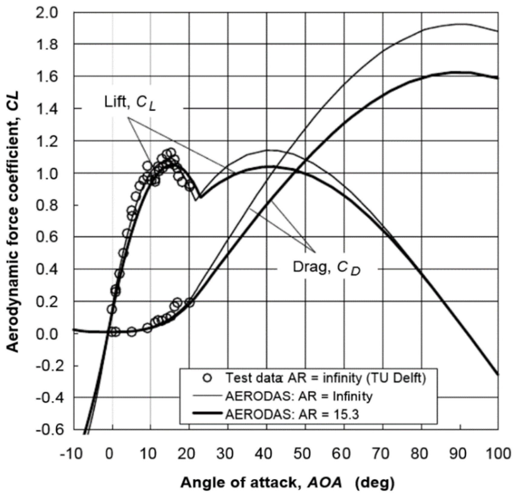
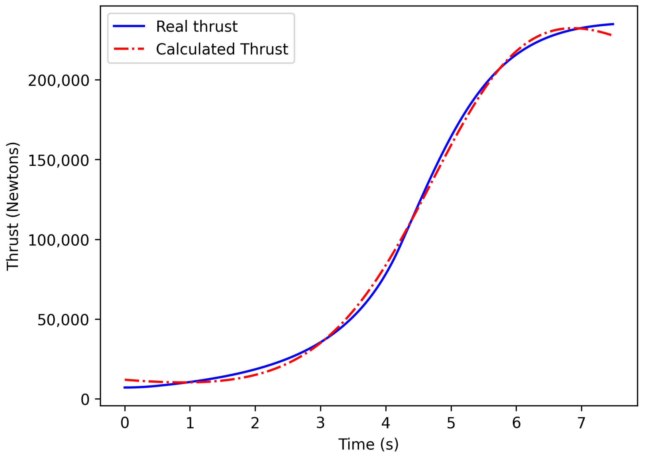
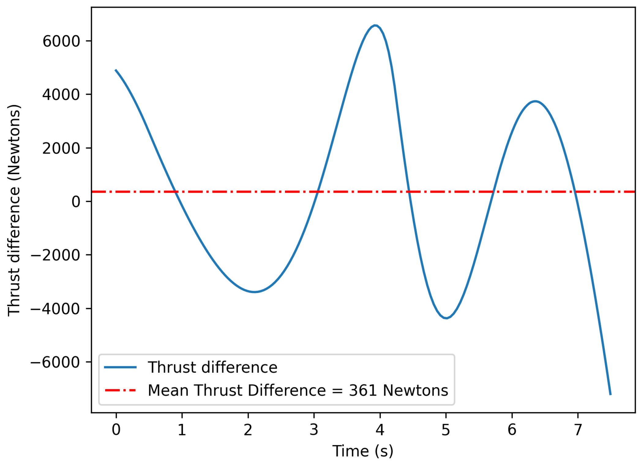
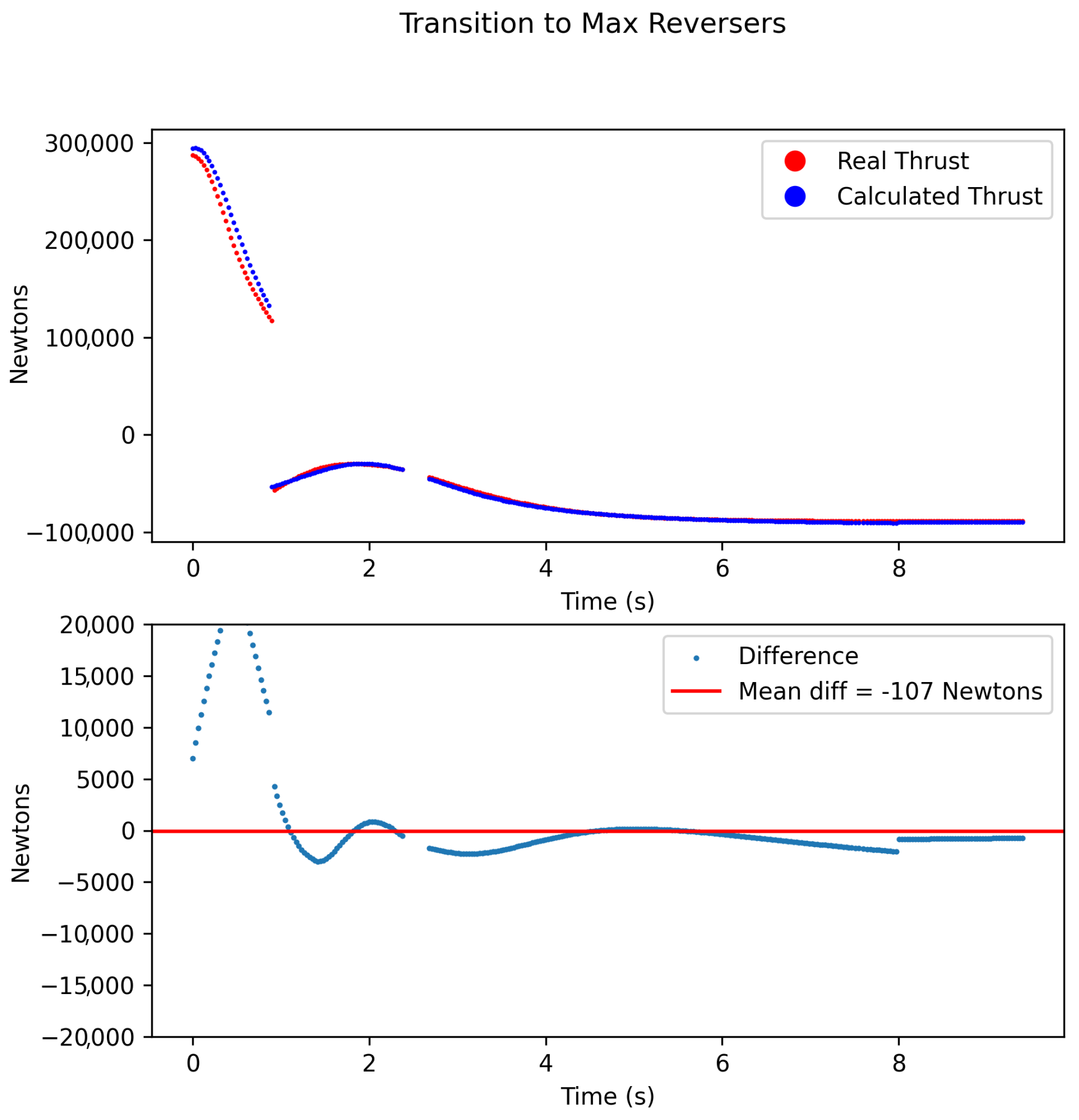
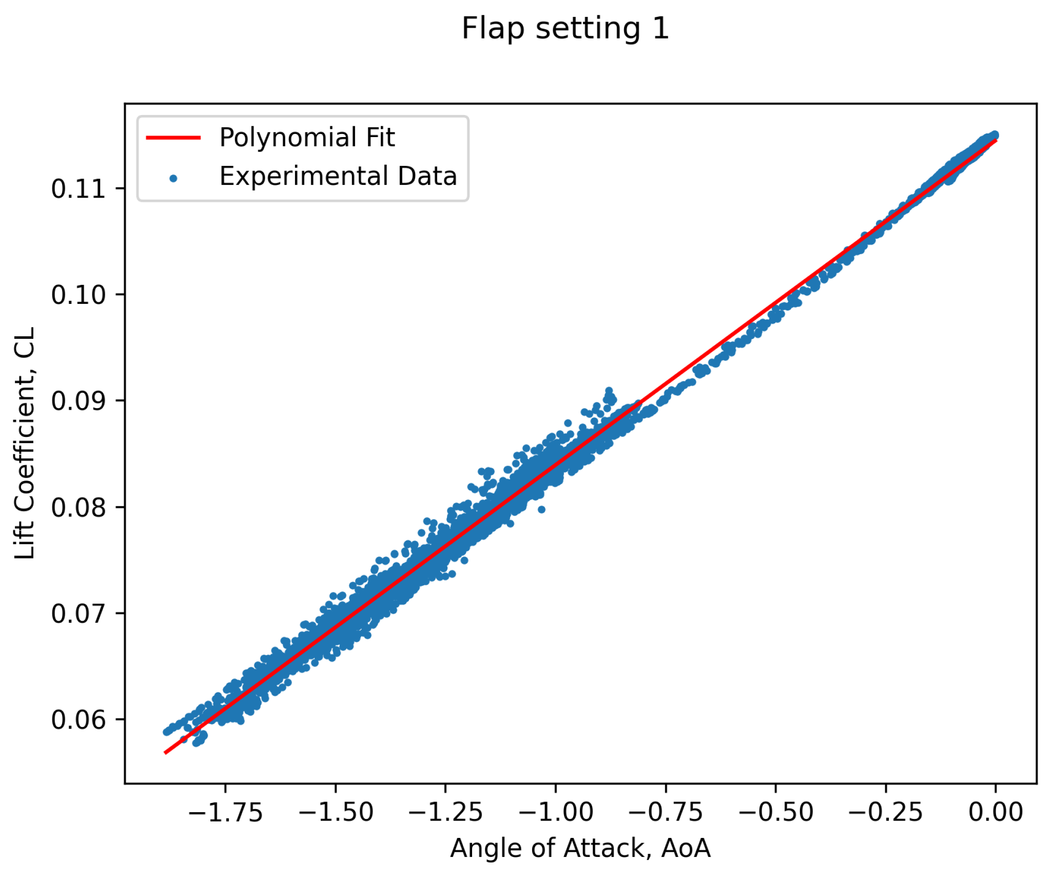
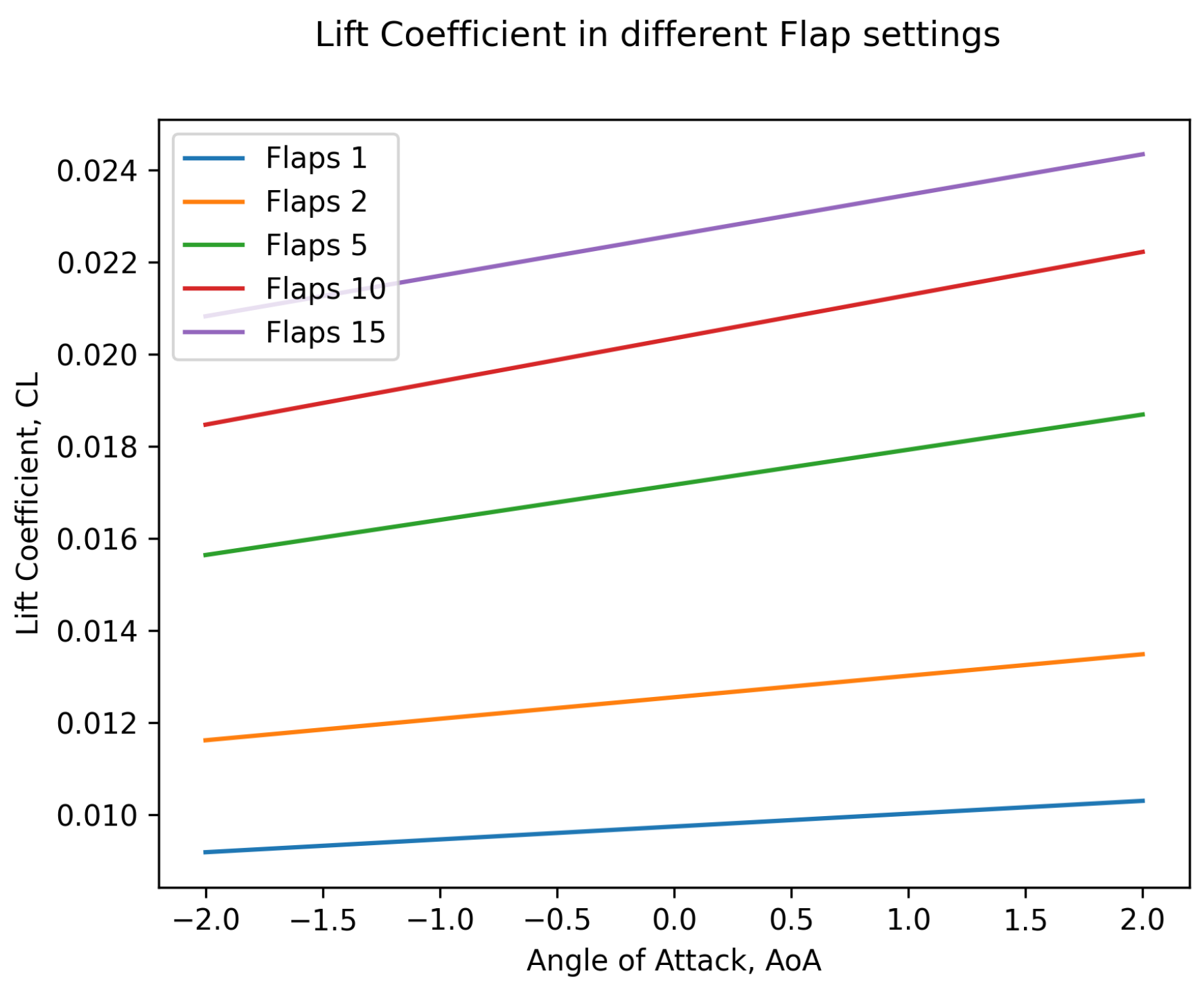
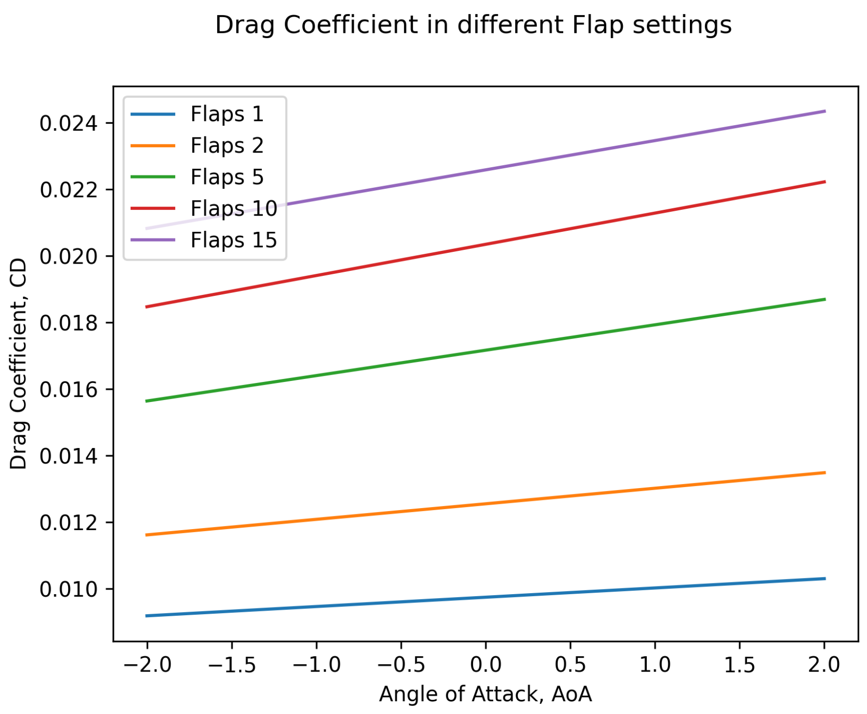
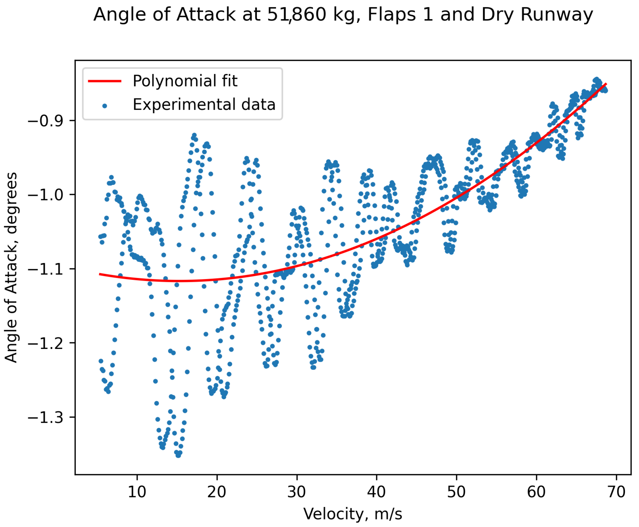

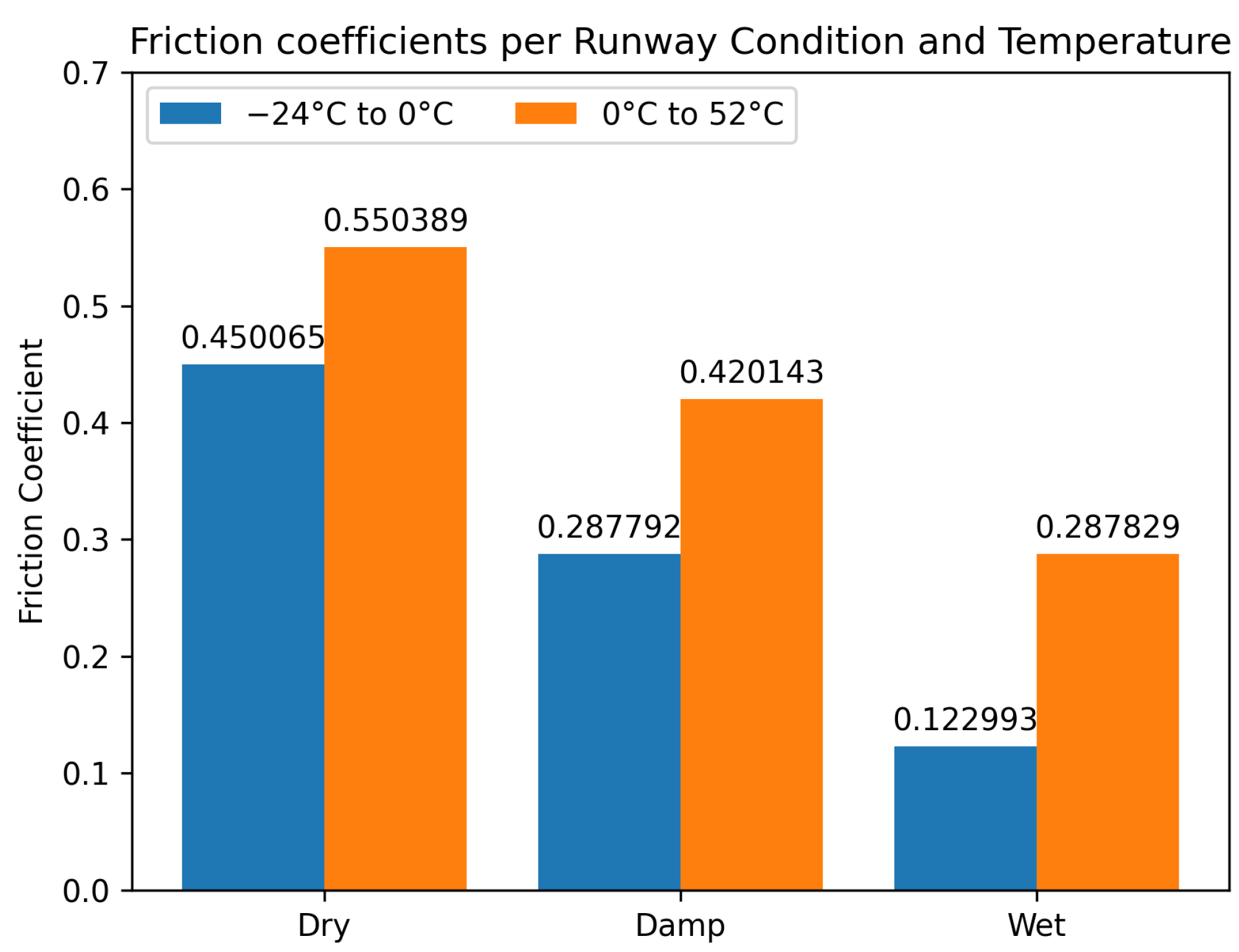
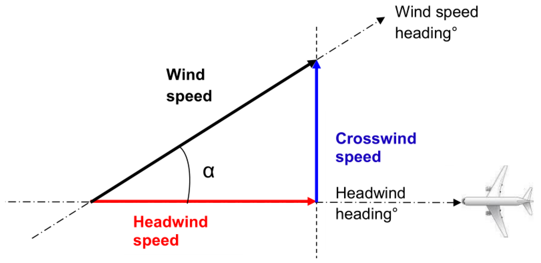
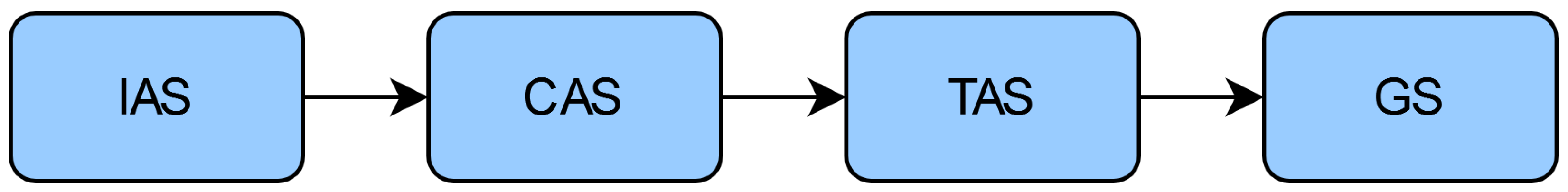
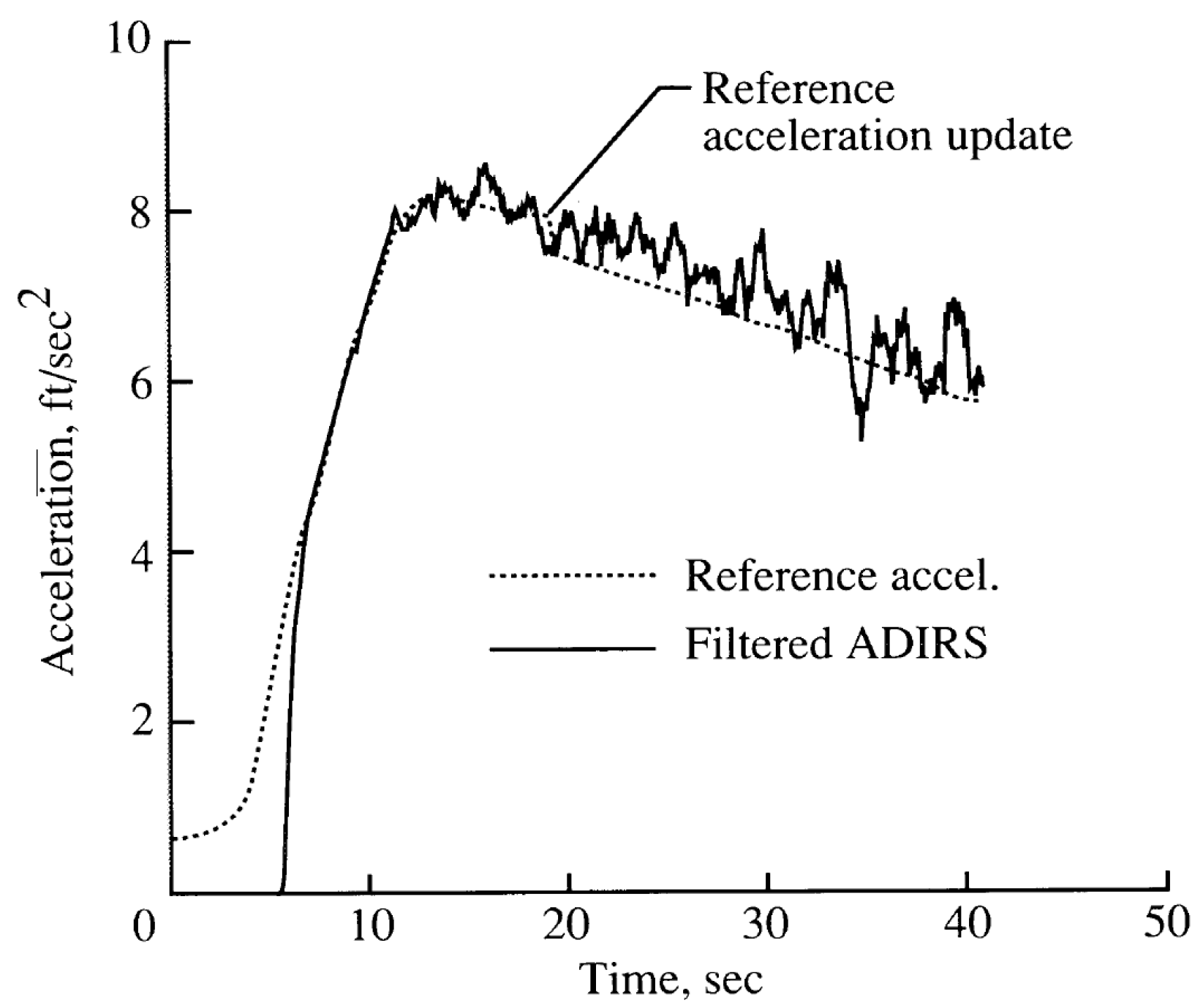
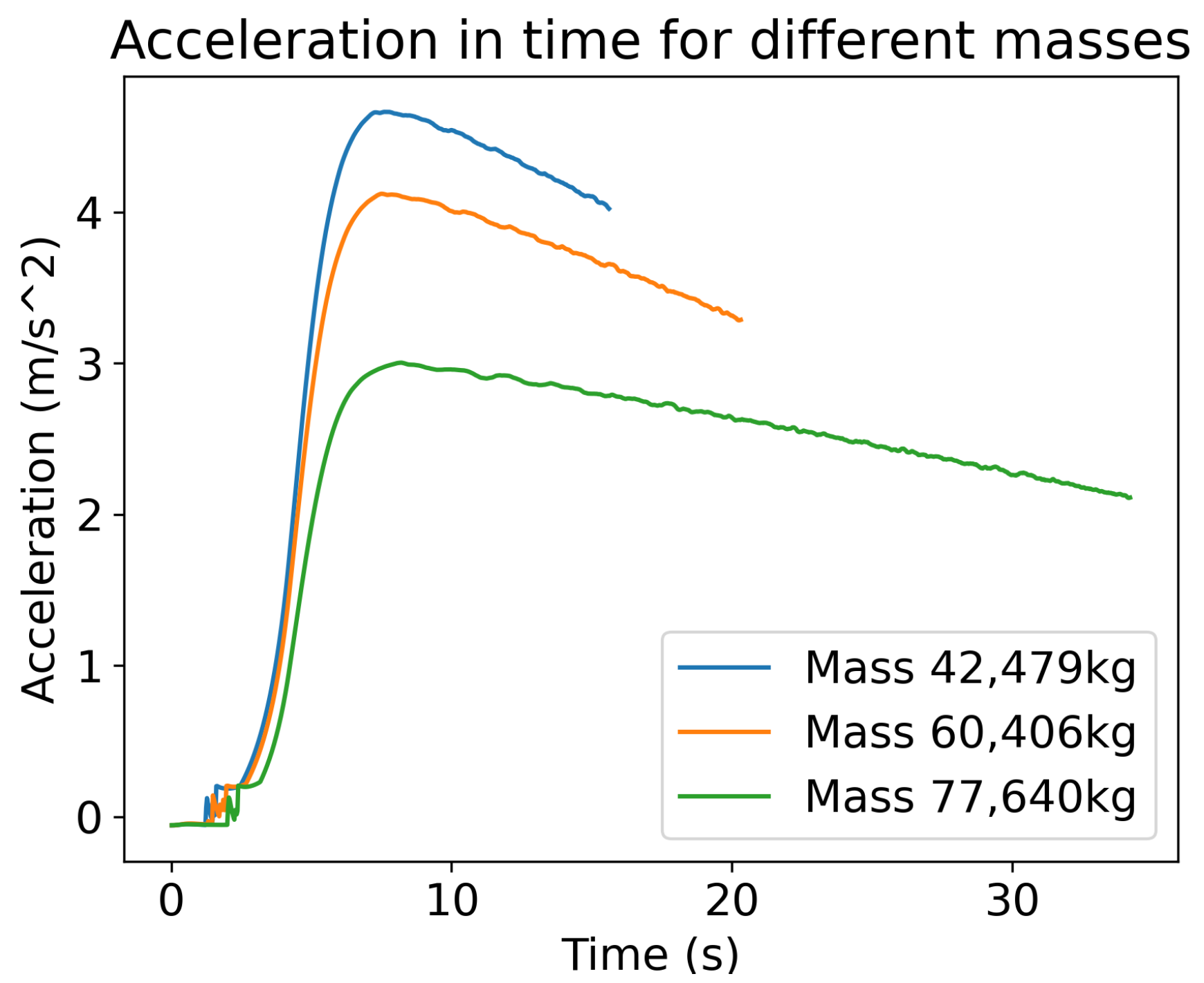
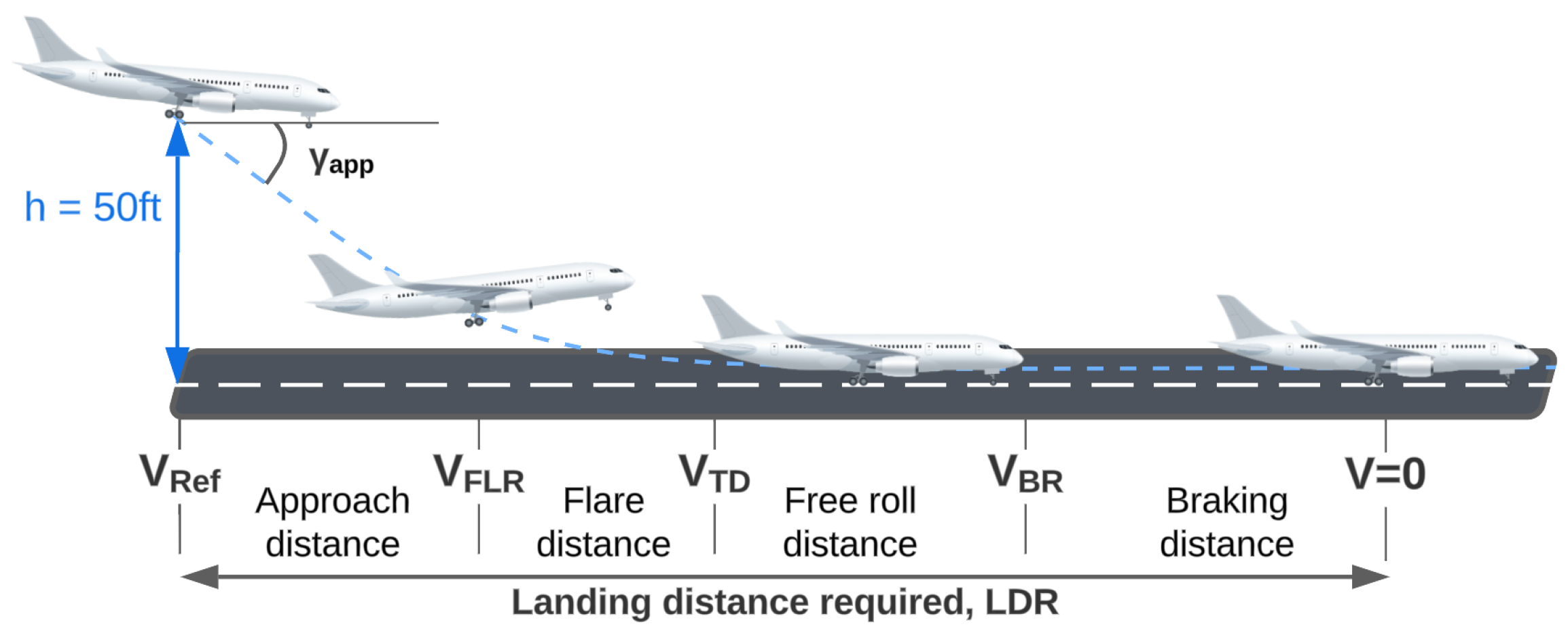
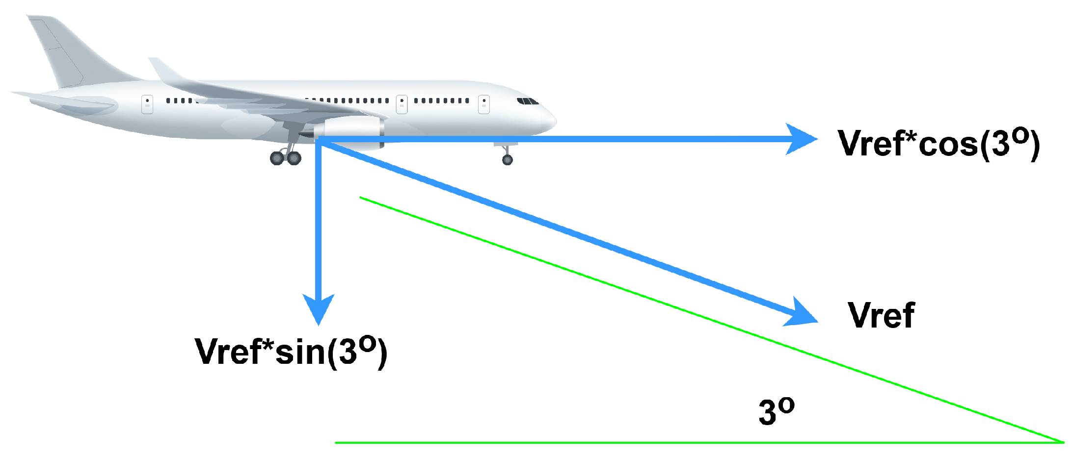

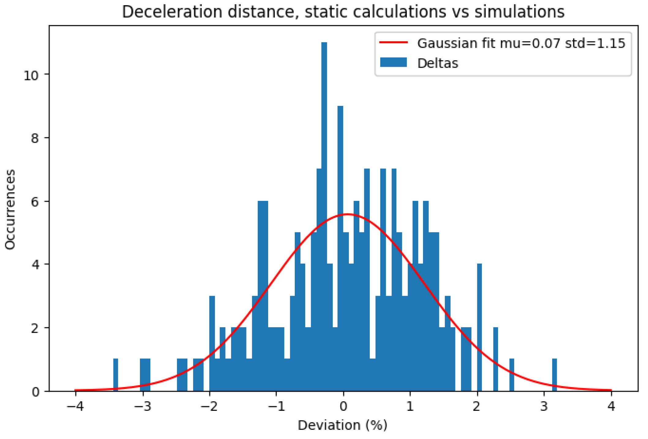
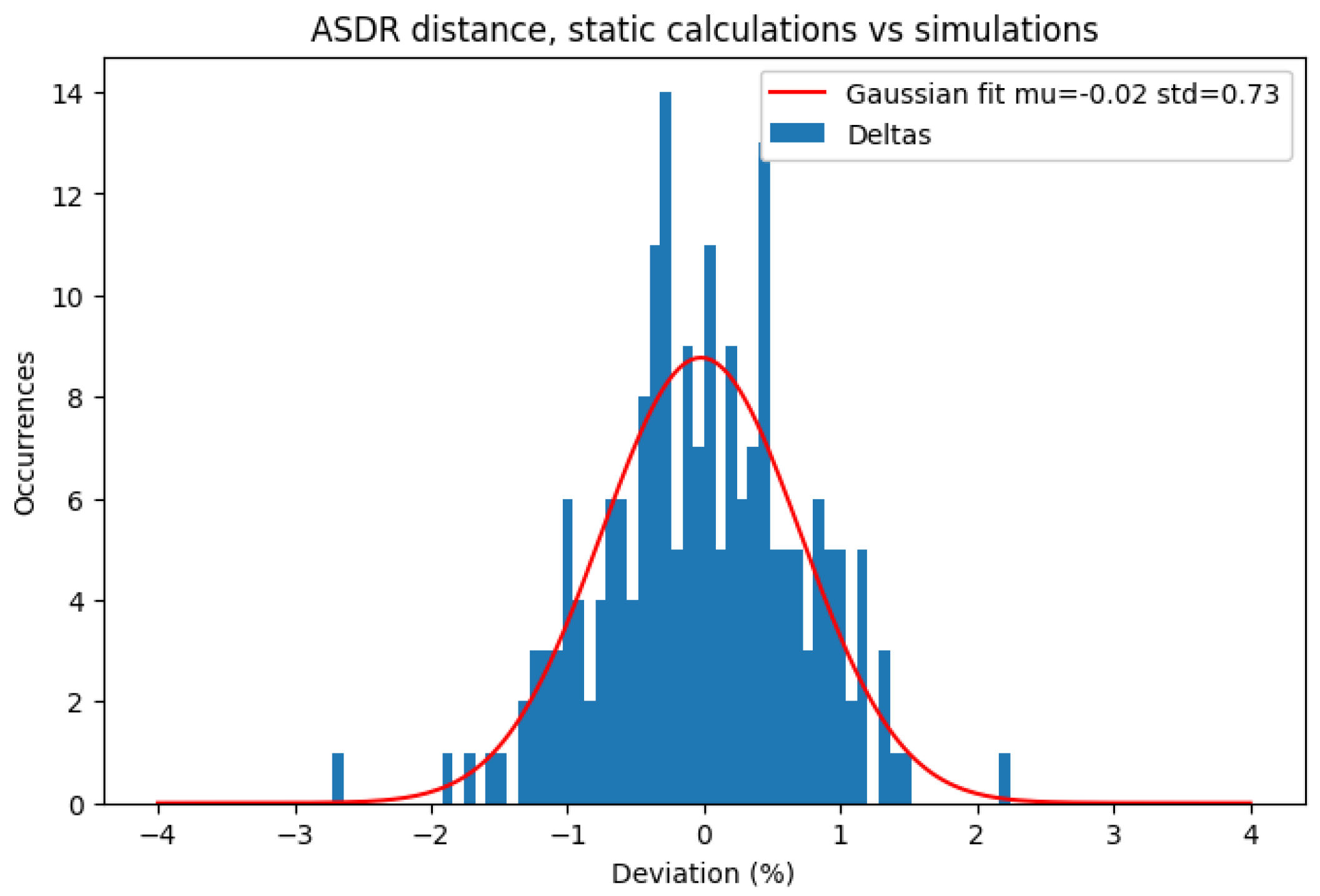
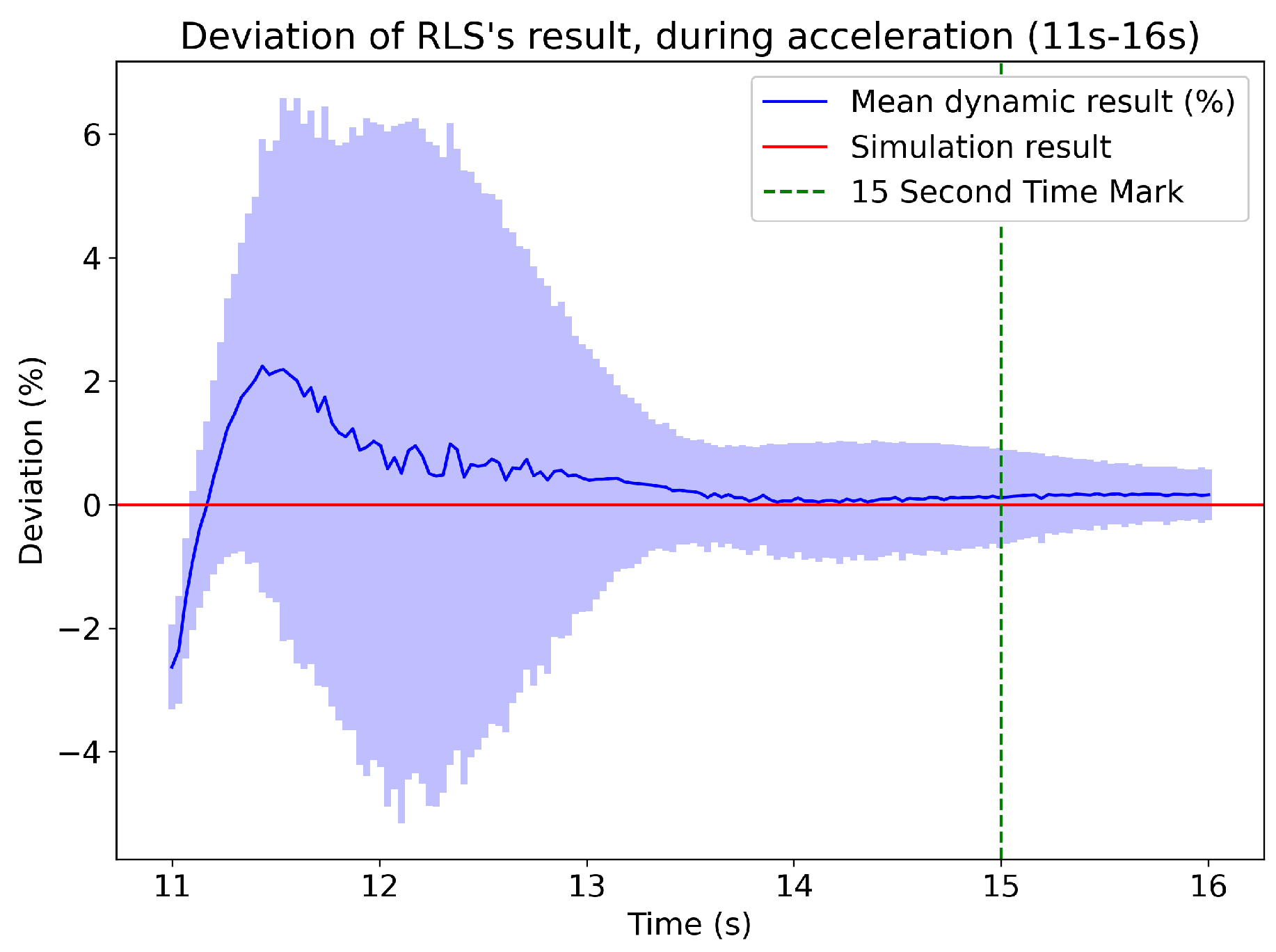
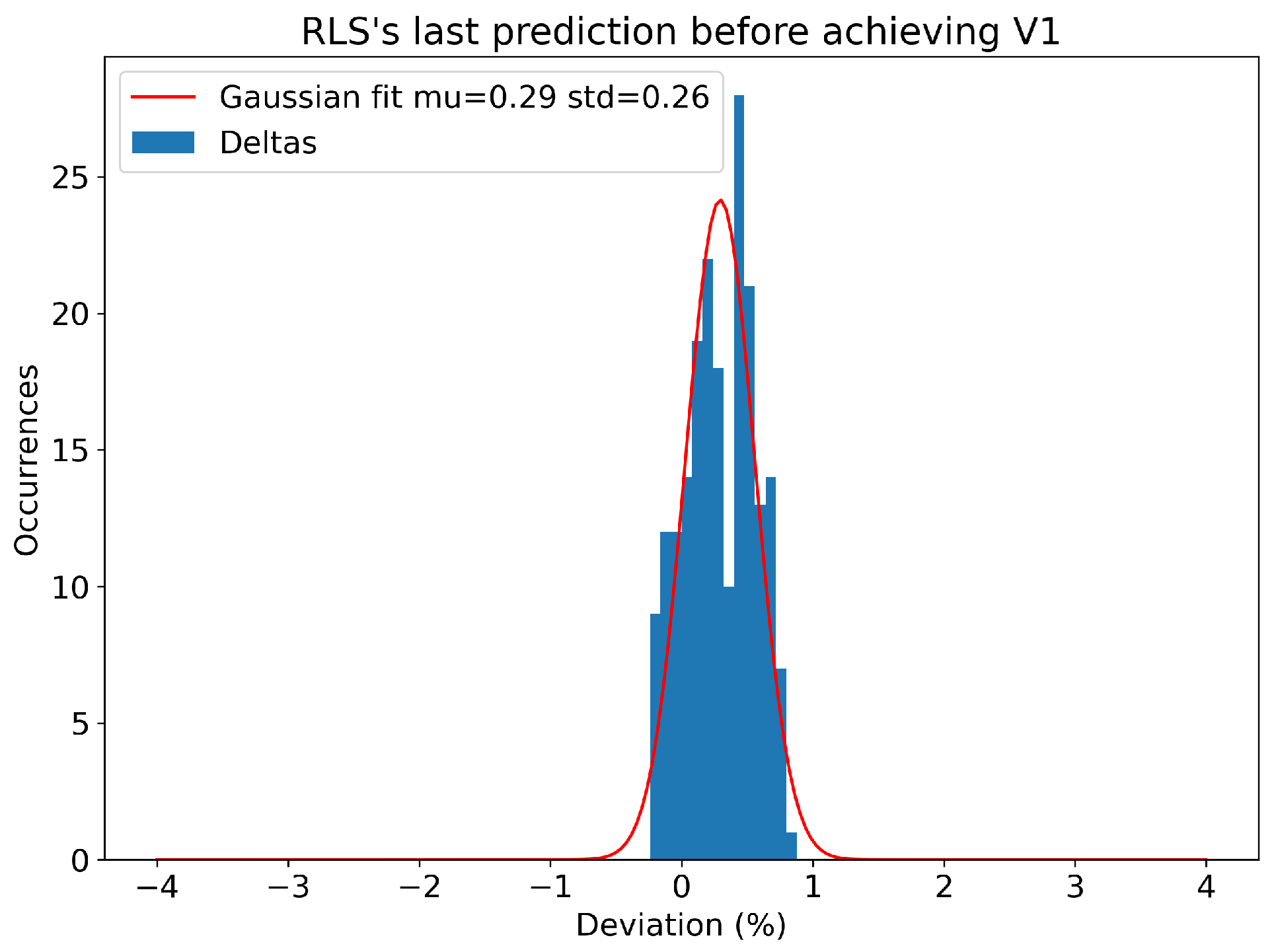
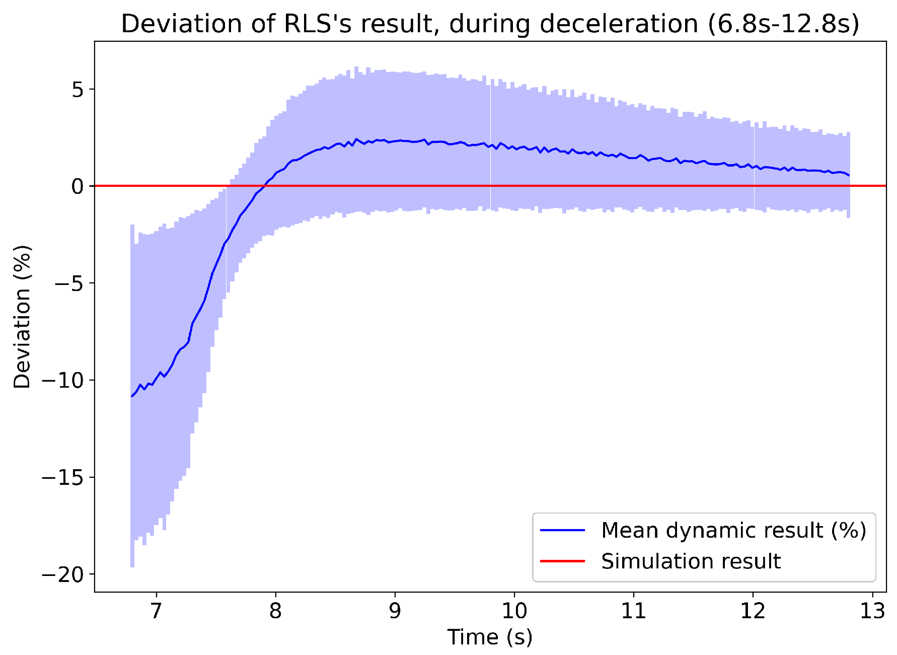


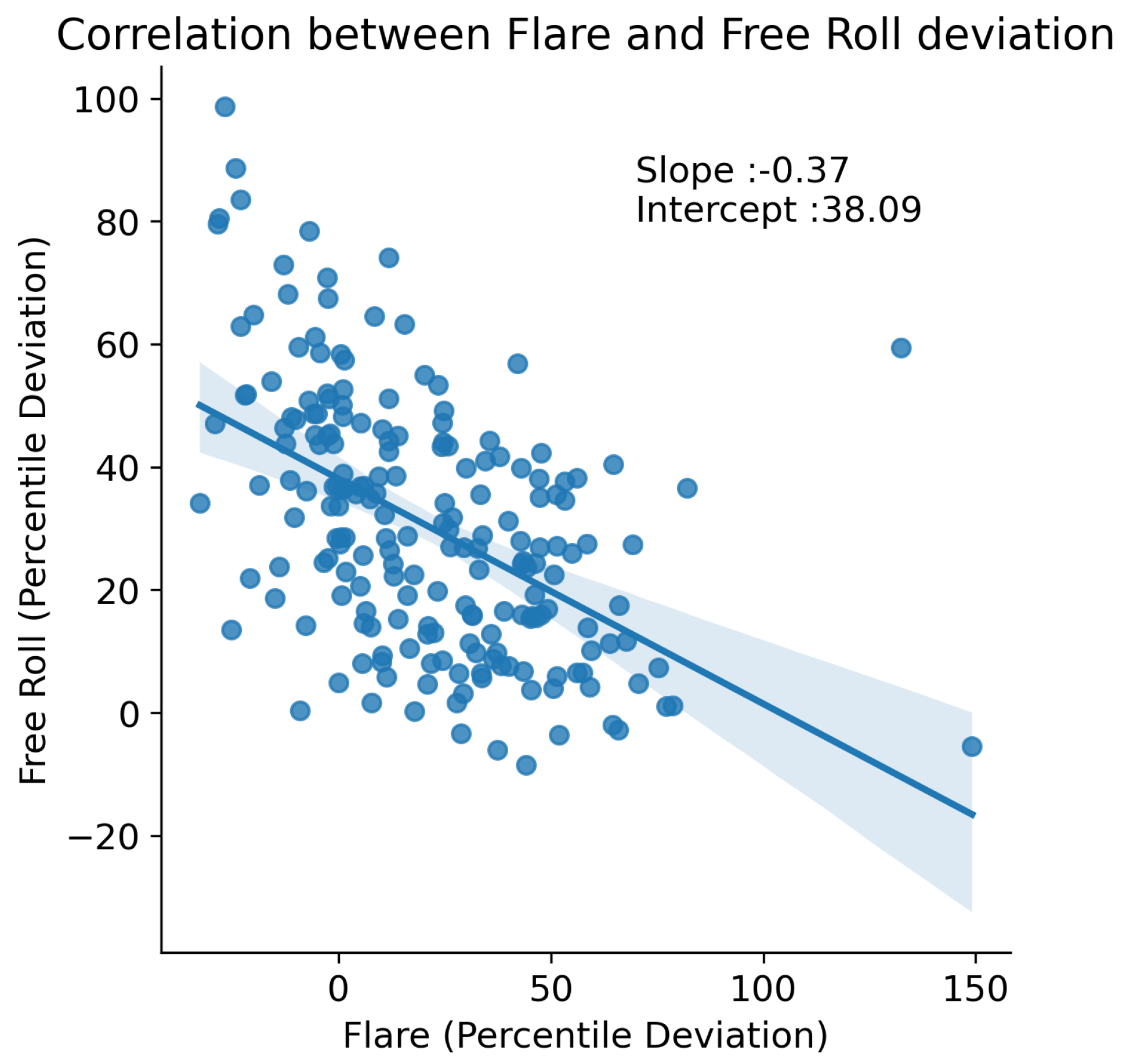
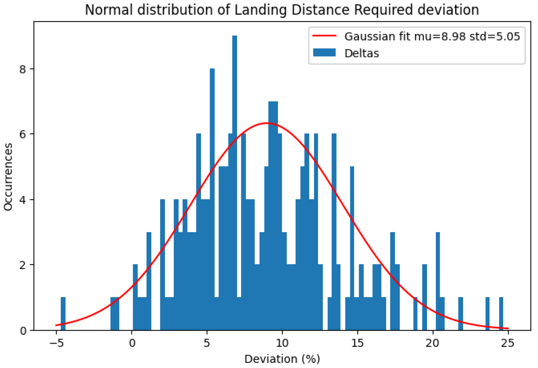
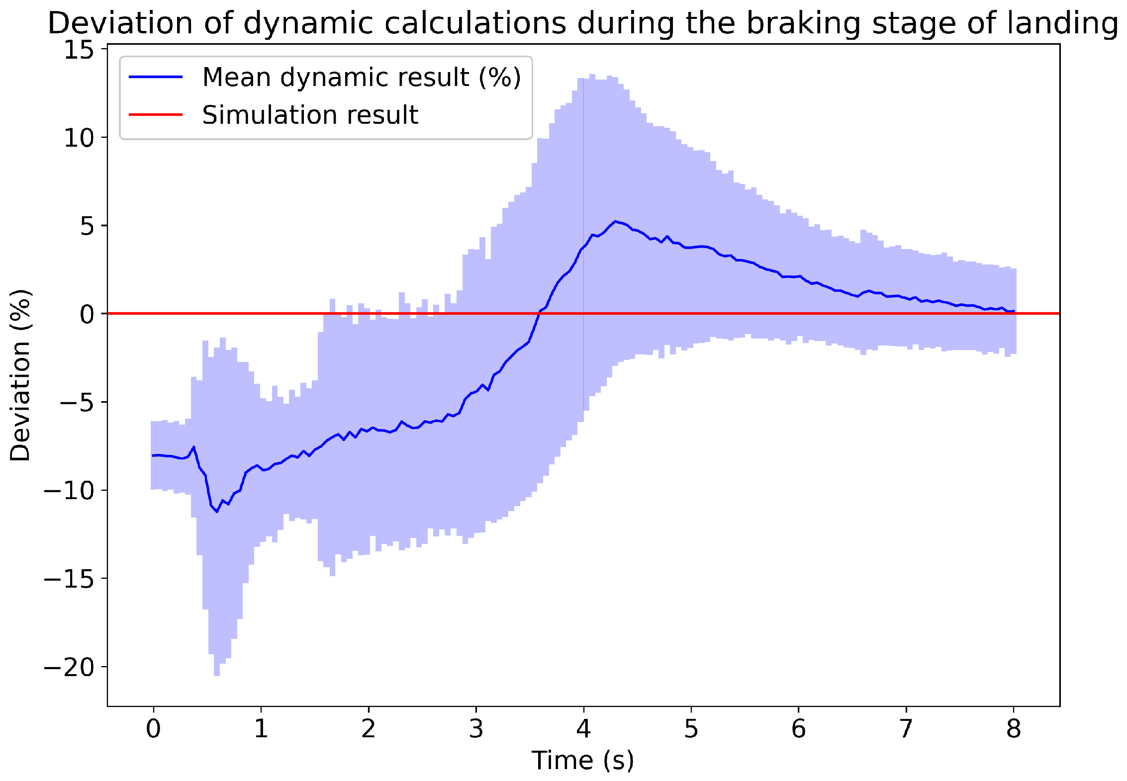
Disclaimer/Publisher’s Note: The statements, opinions and data contained in all publications are solely those of the individual author(s) and contributor(s) and not of MDPI and/or the editor(s). MDPI and/or the editor(s) disclaim responsibility for any injury to people or property resulting from any ideas, methods, instructions or products referred to in the content. |
© 2024 by the authors. Licensee MDPI, Basel, Switzerland. This article is an open access article distributed under the terms and conditions of the Creative Commons Attribution (CC BY) license (https://creativecommons.org/licenses/by/4.0/).