
Impact of Pitch Angle Limitation on E-Sail Interplanetary Transfers


Department of Civil and Industrial Engineering, University of Pisa, I-56122 Pisa, Italy
Aerospace 2024, 11(9), 729; https://doi.org/10.3390/aerospace11090729
Submission received: 7 August 2024
/
Revised: 3 September 2024
/
Accepted: 3 September 2024
/
Published: 6 September 2024
(This article belongs to the Special Issue Advances in CubeSat Sails and Tethers (2nd Edition))
Abstract
:The Electric Solar Wind Sail (E-sail) deflects charged particles from the solar wind through an artificial electric field to generate thrust in interplanetary space. The structure of a spacecraft equipped with a typical E-sail essentially consists in a number of long conducting tethers deployed from a main central body, which contains the classical spacecraft subsystems. During flight, the reference plane that formally contains the conducting tethers, i.e., the sail nominal plane, is inclined with respect to the direction of propagation of the solar wind (approximately coinciding with the Sun–spacecraft direction in a preliminary trajectory analysis) in such a way as to vary both the direction and the module of the thrust vector provided by the propellantless propulsion system. The generation of a sail pitch angle different from zero (i.e., a non-zero angle between the Sun–spacecraft line and the direction perpendicular to the sail nominal plane) allows a transverse component of the thrust vector to be obtained. From the perspective of attitude control system design, a small value of the sail pitch angle could improve the effectiveness of the E-sail attitude maneuver at the expense, however, of a worsening of the orbital transfer performance. The aim of this paper is to investigate the effects of a constraint on the maximum value of the sail pitch angle, on the performance of a spacecraft equipped with an E-sail propulsion system in a typical interplanetary mission scenario. During flight, the E-sail propulsion system is considered to be always on so that the entire transfer can be considered a single propelled arc. A heliocentric orbit-to-orbit transfer without ephemeris constraints is analyzed, while the performance analysis is conducted in a parametric form as a function of both the maximum admissible sail pitch angle and the propulsion system’s characteristic acceleration value.
1. Introduction
An interplanetary spacecraft equipped with an Electric Solar Wind Sail (E-sail) essentially consists of a large space structure made up of a series of long conducting tethers, which are capable of deflecting the charged particles of the solar wind through an artificial electric field that surrounds the vehicle [1]. The conducting tethers [2,3,4], which consist of a series of suitably interconnected metal wires [5,6], deploy from a central body [7,8,9,10] that contains the main subsystems of the spacecraft (such as the power generation system), including the payload whose mass affects the effective value of the available propulsive acceleration for an assigned total tether length [11]. Figure 1 shows the centrifugal deployment process [8] of an E-sail-propelled spacecraft, which is schematized by the main body, the conducting tethers, and the remote units at the very end of each cable. In particular, the deployment of the conducting tethers takes place substantially in a reference plane perpendicular to the direction of the spacecraft angular velocity vector (see the spin direction described by the curved orange arrows in the figure). That plane, which is indicated with a green shaded disk in Figure 1b, is the so-called “sail nominal plane”, which coincides with the plane that formally contains the conducting tethers during the interplanetary flight. Recall that the generic tether bends during flight [12,13], so the sail nominal plane must be considered a sort of reference plane useful for designing the guidance law required to complete the heliocentric transfer.
Over the years, the arrangement of the conducting tethers in a typical E-sail design has evolved from the grid configuration originally proposed by inventor Dr. Janhunen in his two seminal papers [14,15] that sparked the study of this fascinating propellantless propulsion system. In this regard, a review article by Bassetto et al. [16] describes the evolution of the E-sail concept (and the thrust vector mathematical model) up to the state of the art two years ago, while the more recent first edition of the special issue of the journal Aerospace entitled Advances in CubeSat Sails and Tethers [17] collects a series of interesting articles that provide a snapshot of the current state of scientific research regarding this advanced propulsion system, especially from the point of view of the (hopefully) upcoming flight tests [18,19,20]. In this context, Figure 2 shows an artistic impression of a single-tether E-sail that, after the first attempts unfortunately failed [21,22,23,24,25], could soon be used to achieve the first in situ evidence of the potentialities of this propulsion system concept through the use of a CubeSat [26,27,28] inserted in a high-elliptic lunar orbit, which allows the (single) conducting tether to interact with the solar wind flow [29,30]. Finally, from the point of view of the geometric arrangement of the E-sail conducting tethers, very recently, Bassetto et al. [31] analyzed the potentialities of a sort of “web-shaped” E-sail, in which a number of (closed) azimuthal conducting tethers connect the classical radial tethers deployed from the spacecraft central body. In particular, Ref. [31] analyzed the characteristics of the thrust vector of a web-shaped E-sail by using a semi-analytical approach, which allows the designer to evaluate the impact of the presence of the azimuthal tethers on the propulsive performance with a set of simple, closed-form equations.
An axially symmetric E-sail is theoretically able to generate an outward radial thrust, that is, a thrust vector directed along the Sun–spacecraft line, when the sail nominal plane is substantially perpendicular to the direction of the solar wind flow [32]. This type of Sun-facing orientation, which can be passively maintained by the axially symmetric E-sail, is modified when the desired steering law requires the presence of a transverse (i.e., a non-radial) component of the propulsive acceleration [33]. In fact, the presence of a transverse thrust component is a necessary condition to achieve a transfer between two heliocentric Keplerian orbits that do not share the same value of the semilatus rectum. In this context, the recent work of the author [34] analyzes the optimal performance of an E-sail facing the Sun in a two-dimensional transfer between a generic Keplerian elliptic orbit and a circular one whose radius, in fact, has a value equal to the semilatus rectum of the initial (elliptic) parking orbit. Figure 3 shows the case of a zero pitch angle (i.e., the Sun-facing configuration), and the more generic situation in which the pitch angle is different from zero. Note in Figure 3b as the E-sail-induced thrust vector lies between the Sun–spacecraft line and the direction perpendicular to the sail nominal plane in the case of a non-zero value of the sail pitch angle.
The generation of a transverse thrust component is strictly connected to the possibility of tilting the sail nominal plane with respect to the Sun–spacecraft (radial) line, in order to obtain a value of the sail pitch angle different from zero [35,36]. This variation in the inclination of the sail nominal plane with respect to the (passively stable) Sun-facing configuration requires a specific attitude control law whose performance, in terms of system settling time, depends directly on the desired (target) value of the sail pitch angle [37]. The thrust vectoring of a spinning E-sail-propelled spacecraft is, in fact, a complex task, which requires a precise design of the attitude control system as thoroughly discussed in the two interesting papers by Toivanen and Janhunen [38,39] that analyzed this specific important problem by using an elegant analytical approach. In this regard, the E-sail-related scientific literature contains more recent and useful works [40,41] which investigate the connection between a generic E-sail attitude maneuver and the spacecraft response from the structural viewpoint, taking the intrinsic flexibility of such a large space structure into account [42,43,44].
From the perspective of attitude control system design, a constrained (and generally small) value of the target sail pitch angle could improve the effectiveness of the maneuver for the variation in the inclination of the sail nominal plane at the expense, however, of a worsening of the orbital transfer performance in terms of the required total flight time [45]. The aim of this paper is to investigate the effects of a constraint on the maximum value of the sail pitch angle, on the performance of a spacecraft equipped with an E-sail propulsion system in a typical interplanetary mission scenario [46]. In particular, the spacecraft mission performance is evaluated in terms of the minimum flight time for an assigned value of the maximum admissible sail pitch angle. In this context, the spacecraft guidance law is determined in a classical optimization framework by considering a mission scenario which is consistent with a three-dimensional, E-sail-based, interplanetary transfer from Earth to one of the other three terrestrial planets [47]. In particular, a heliocentric orbit-to-orbit transfer without ephemeris constraints is analyzed, while the performance analysis is conducted in a parametric form as a function of both the maximum admissible sail pitch angle and the propulsion system’s characteristic acceleration value. During flight, the E-sail propulsion system is considered to be always on so that the entire transfer can be considered a single propelled arc without any coasting phases. This specific situation allows the designer to further simplify the (optimal) guidance law because, during the whole transfer, the spacecraft control vector is formed only by the components of the propulsive acceleration unit vector. In other words, the guidance law for interplanetary transfer requires the evaluation, at each instant of time, of two independent scalar terms, one of which is precisely the constrained value of the pitch angle of the sail nominal plane.
In this context, the minimum (constrained) flight time is compared with the truly optimal (unconstrained) transfer time in order to evaluate the relative impact of the presence of a sail pitch angle limitation on the mission performance. In particular, the truly optimal transfer times, which are calculated to provide a benchmark, extend the E-sail literature because they are evaluated considering a single propulsion arc during the flight, i.e., they are the output of a simplified steering law which can be used to reduce the size of the E-sail control vector. Starting from the elegant thrust vector model proposed by Huo et al. [48], and taking the results of the optimization process described in a companion paper by the author [49], Section 2 discusses the E-sail control law in the presence of the constraint on the sail pitch angle. Section 3 illustrates the corresponding numerical simulations and a set of suitable graphs which allows the designer to quickly estimate the (percentage) performance degradation in the three interplanetary scenarios considered in this work. Finally, Section 4 concludes this work by summarizing the main results obtained.
2. Mathematical Preliminaries and Thrust Vector Analytical Model
This section discusses the E-sail thrust vector model in the presence of (1) a constraint on the maximum value of the sail pitch angle along the transfer orbit, and (2) a single propelled arc during the interplanetary flight between two assigned (Keplerian) heliocentric orbits. Furthermore, this section briefly indicates the mathematical approach used to obtain the optimal (constrained) transfer trajectory in the generic, orbit-to-orbit, heliocentric mission scenario. In the latter case, we avoid describing in detail the mathematical model used in the optimization process, to streamline the discussion of the proposed model. In any case, a detailed indication of the recent literature where the interested reader can find the related mathematical model is included in the text.
2.1. Analytical Model of the Propulsive Acceleration Vector
The expression of the propulsive acceleration vector used in this work is a simplified version of the one obtained by Huo et al. in 2018 [48] using a geometric (and analytical) approach. In particular, the formula obtained by Huo et al. is able to relate the propulsive acceleration vector generated by the E-sail both to the Sun–spacecraft unit vector and to the attitude of the sail nominal plane with respect to a classical orbital reference frame. This attitude is essentially described by the unit vector normal to the sail nominal plane in the direction opposite to the Sun.
In fact, bearing in mind that the E-sail propulsion system is always switched on during the flight, the elegant and compact Equation (17) by Ref. [48] simplifies as
where r is the distance of the spacecraft from the Sun, is a reference distance, and is the E-sail typical performance parameter, i.e., the sail characteristic acceleration [50]. The latter is defined, borrowing the nomenclature used in the field of solar sails [51,52,53], as the maximum value of the magnitude of the vector when the distance of the probe from the Sun is one astronomical unit, that is, when . Note that, at an assigned distance from the Sun, the maximum magnitude of the propulsive acceleration vector is obtained if , i.e., if the E-sail orientation is Sun-facing; see Figure 3a. To be precise, it should be noted that the expression of the propulsive acceleration vector given by Equation (1) is strictly valid if the distance of the vehicle from the Sun is around one astronomical unit since the mathematical model that underlies this expression of is consistent with the discussion reported in Refs. [1,38,39]. However, in the absence of a more suitable thrust model and taking into account the simplicity of the one proposed by Huo et al. [48], in the remainder of this work, the expression of given by the previous equation will be considered valid even when the distance of the spacecraft from the Sun is considerably different from .
As expected, Equation (1) indicates that cannot be zeroed during the flight (recall that by assumption) except in the trivial case of . The dependence of from the sail pitch angle can be highlighted by introducing a typical Radial-Transverse-Normal reference frame (RTN), like that sketched in Figure 4 in which is the radial unit vector, is the transverse unit vector, and is the normal unit vector. This RTN reference system is quite conventional, but we point out that the origin of the frame coincides with the spacecraft’s center of mass , while coincides with the plane of the spacecraft osculating orbit during the interplanetary flight.
The propulsive acceleration vector can be written as a function of the sail pitch angle by using Equation (1) and the scheme of Figure 5, which shows the generic orientation of the normal unit vector in the RTN reference frame. In particular, Figure 5 indicates two important angles that define the E-sail control vector, namely, the (already defined) sail pitch angle and the sail clock angle , which gives the orientation of the projection of in the plane .
Accordingly, using Equation (1) to express vector and bearing in mind the scheme of Figure 5, one obtains the radial (), transverse (), and normal () components of the propulsive acceleration vector as
which can be more conveniently rewritten in a dimensionless form (the tilde superscript will be used in the rest of the paper to indicate the dimensionless version of a given term) as
In a typical unconstrained case, the sail pitch angle ranges from zero to , i.e., , so that the variation in the three dimensionless components of the propulsive acceleration vector gives the so-called “force bubble” [54] shown in Figure 6, that is, the bubble-shaped surface (in this specific case, it is a sphere) on which the tip of the dimensionless vector is constrained to lie. In particular, the force bubble drawn in Figure 6 refers to the special case where , while the presence of a solar distance different from does not modify the shape of the bubble. In Figure 6, recall that the direction of propagation of the solar wind coincides with the direction of the z-axis, that is, the Sun belongs to the vertical axis and is located in the negative half-space.
In a constrained case in which the sail pitch angle ranges in the interval , where is the assigned maximum value of the pitch angle, the shape of the force bubble changes with respect to the scheme of Figure 6. In particular, the reduction in the value of results in a reduction in the size of the force bubble as highlighted in Figure 7, which shows, for illustrative purposes, the four cases of . Note from Figure 7 that in the (rather limiting) case of , the force bubble becomes a small spherical cap, which indicates that, as expected, for a small value of , the propulsive acceleration vector is essentially radial with a very small transverse component. This last aspect, as discussed above, is a limiting factor in the heliocentric transfer between two orbits with different values of the semilatus rectum.
The constrained thrust vector model given by Equations (2)–(4) with and can be used to describe the influence of the E-sail-induced acceleration in an optimized (from the flight time point of view) interplanetary orbit transfer. In this regard, the recent literature already contains the complete (unconstrained) mathematical model for trajectory optimization in the heliocentric scenario. This latter model can be easily adapted to this constrained case as briefly discussed in the next section.
2.2. Brief Notes on Trajectory Optimization in Presence of Pitch Angle Constraint
The optimization of the three-dimensional transfer trajectory in the presence of a geometric constraint on the maximum value of the sail pitch angle can be studied by easily adapting the mathematical model illustrated by the author in an open-access companion paper [49] appearing in this same Special Issue.
More precisely, the very recent Ref. [49] analyzes the three-dimensional, heliocentric, rapid orbit cranking maneuver of an E-sail propelled spacecraft by assuming a circular parking and target orbit. In particular, the mathematical model proposed in [49] uses the dimensionless modified equinoctial orbital elements [55] to describe the spacecraft dynamics, a classical indirect approach [56,57] to obtain the rapid transfer trajectory, and the Pontryagin’s maximum principle [58] to derive the optimal guidance law during the interplanetary flight.
As regards the mathematical description of the E-sail-based spacecraft heliocentric dynamics, the model discussed in [49] can be applied directly with the only difference concerning the initial and final conditions, which, in the case treated in this paper, must be consistent with the specific interplanetary mission scenario analyzed. As discussed in the next section, the constrained thrust model is used here to analyze the E-sail performance in a set of interplanetary orbit-to-orbit transfers, in which the spacecraft parking (or final) orbit coincides with the heliocentric trajectory of the Earth (or the target planet). Accordingly, when the initial value of the time is set to zero, Equation (21) of Ref. [49] is substituted by
where are the five dimensionless modified equinoctial elements that define the shape and orientation of the Earth’s heliocentric orbit, while is the variable adjoint to the state L. In particular, the value of the set was obtained using the data retrieved from the well-known JPL Horizon system on 1 August 2024. Note that in Equation (8), the condition indicates that the starting point on the parking orbit is not constrained, and is an output of the optimization process. The spacecraft final conditions, that is, the conditions to be reached at the final time , which in Ref. [49] are given by Equations (33) and (34), are now expressed as
where depend on the orbital characteristics of the target planet (the values have been retrieved again from the JPL Horizon system on 1 August 2024), while is the final value of the Hamiltonian function. Even at the final time, the spacecraft angular position along the target orbit is left free [indeed, one has in Equation (9)] so that the interplanetary transfer is considered ephemeris-free.
The optimal control law is a simplified version of the one described in Ref. [49] because the E-sail propulsion system is always switched on during the transfer. In this case, in fact, we must determine the (optimal) time variation in the two control angles and , taking into account the constraint . As for the optimal value of the clock angle, the results of the unconstrained case are still valid, and one can directly take the value given by Equations (27) and (28) of Ref. [49]. On the other hand, the expression of the optimal pitch angle given by Equation (30) of Ref. [49] cannot be used in this context because it does not take into account the presence of the constraint on its maximum value. However, Equation (30) of Ref. [49] is still a good starting point to obtain the optimal sail pitch angle. In fact, the presence of the constraint gives the following expression of the optimal value of :
where is given by Equation (30) of Ref. [49]. The boundary value problem associated to the optimization procedure has been solved using a shooting method, in which the initial value of the unknown costates have been estimated by adapting the recent procedure proposed by the author in Ref. [59]. The numerical results, for the three mission scenario selected, are illustrated in the next section.
3. Orbital Simulations and Numerical Results
The impact of the constraint on the maximum value of the sail pitch angle is evaluated considering three interplanetary scenarios, namely, three-dimensional Earth–Mars, Earth–Venus, and Earth–Mercury transfers. The orbital elements of the four celestial bodies involved in the numerical analysis are summarized in Table 1. In all selected mission scenarios, the spacecraft has a canonical value of the characteristic acceleration, namely, = 1 mm/s, which corresponds to approximately of the gravitational acceleration of the Sun at one astronomical unit distance from the star. The procedure, of course, can be applied for a generic value of as will be discussed in the last part of this section.
The first step of this analysis is to determine the optimal transfer performance in the unconstrained case, which essentially corresponds to selecting in the automatic routines that optimize the constrained version of the interplanetary transfer. In this important case, the numerical results in terms of the minimum (unconstrained) flight time and the maximum (or minimum) value of the sail pitch angle reached during the orbit-to-orbit interplanetary transfer [or ] are summarized in Table 2. Recall that the propulsion system is always switched on during the flight.
The data reported in Table 2 are consistent with the graphs of Figure 8, Figure 9 and Figure 10, which show the time variation in the two control angles in the three selected interplanetary mission scenarios. The corresponding optimal transfer trajectory is reported (black line) in Figure 11, Figure 12 and Figure 13 by employing a typical heliocentric–ecliptic reference frame with the origin O in the center-of-mass of the Sun [60] and the distances of the axes expressed in astronomical units. Note that the z-axis in Figure 11, Figure 12 and Figure 13 is intentionally exaggerated to better highlight the three-dimensionality of the interplanetary transfer analyzed by the optimization routines. According to Figure 13, it is noted that, even with a medium-high value of the characteristic acceleration such as the one used in the simulations, the optimal transfer without constraints towards the orbit of Mercury is rather complex and requires more than two complete revolutions around the Sun before being completed. On the other hand, the corresponding optimal guidance law is rather simple, and during the flight, the (optimal) value of the sail pitch angle “oscillates” around the value that maximizes the non-radial component of the propulsive acceleration vector; see Equations (6) and (7).
The impact of a constraint on the maximum value of the sail pitch angle is analyzed by calculating the optimal (constrained) interplanetary transfers when the pitch angle ranges in the interval . Indeed, the limiting case of gives the same results as the unconstrained scenario, while a value of gives an extremely high flight time when compared to the one obtained in the unconstrained case. Note that the other limiting case of refers to a Sun-facing flight, where the propulsive acceleration vector is purely radial at every instant of time. In that case, interplanetary transfer is physically impossible because the Sun-facing flight preserves the value of the semilatus rectum, whose value coincides with that of the heliocentric parking orbit (i.e., of the Earth). In any case, an analytical study of the heliocentric motion of a Sun-facing E-sail is presented in Ref. [61].
The numerical results of the constrained optimization process are summarized in Figure 14 for the three interplanetary mission scenarios selected in this work.
In particular, the relative variation in the flight time with respect to the unconstrained case is evaluated by introducing a new dimensionless parameter D defined as
where is the minimum flight time obtained in the unconstrained case (the value of such time is summarized in Table 2), while is the value of the optimal flight time obtained in the constrained case as a function of . For example, a value of indicates that, for the selected value of , the constrained flight time is greater than the value obtained when the sail pitch angle is free to change during the transfer.
According to Figure 14, we note that the shape of the function is similar for the three orbit-to-orbit transfers, while the actual value of D for a given maximum sail pitch angle is strictly dependent on the specific scenario. More precisely, the value of D remains equal to zero until the value of becomes smaller than the value of given in Table 2. Indeed, from the numerical results viewpoint, a case in which is substantially unconstrained because the constraint is not active. On the other hand, we observe that when approaches the value of , the degradation of the transfer performance becomes very evident and the flight time increases by more than thirty percent in the Earth–Mars scenario, while D settles at about sixteen percent in the Earth–Mercury scenario.
For example, in the Earth–Mars scenario where the constrained minimum flight time is roughly when , the time variation in the two control angles is shown in Figure 15. Note that the sail pitch angle is equal to the maximum allowable value of throughout almost the entire interplanetary transfer (the to be right), while the clock angle varies over the entire allowable range during the flight. Similar considerations can be made for the other two mission scenarios considered in this work.
Numerical simulations also highlight that the worsening of the performance obtained in the passage from the unconstrained to the constrained model also depends on the value of the characteristic acceleration considered. This aspect is briefly illustrated in the next subsection.
Effect of the Value of the Characteristic Acceleration
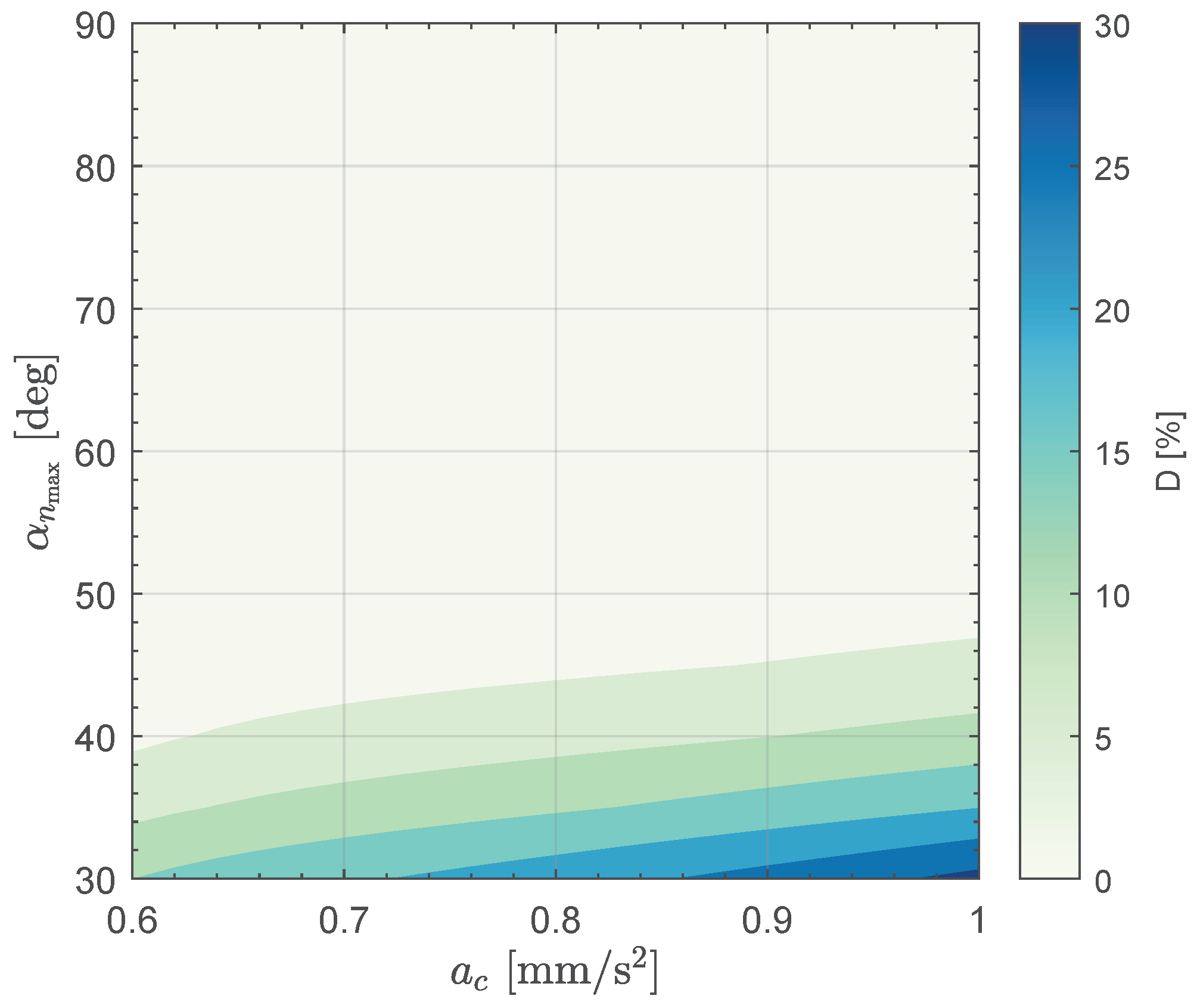
The value of the spacecraft characteristic acceleration influences the performance degradation (in terms of flight time) due to the presence of a constraint on the maximum sail pitch angle. To investigate this aspect, we use a parametric approach to study the Earth–Mars mission scenario, where both the maximum value of the sail pitch angle and the characteristic acceleration vary in the range and , respectively. Note that the case of corresponds to a decrease of from the value used in the simulations discussed in the first part of this section, i.e., = 1 mm/s.
The optimal flight time in the unconstrained case is a function of only, while in the constrained case is a function of both and . In other terms, the dimensionless performance parameter D defined by Equation (11) is now a function of the two terms , that is, one has . Accordingly, the function is a surface whose shape can be numerically obtained by solving a suitable number of optimization problems. The results of the numerical simulations of the optimal transfer trajectories are summarized in Figure 16 and Figure 17, where the dependence of the degradation parameter D on the value of (for an assigned ) can be observed.
4. Conclusions
The thrust vectoring of an interplanetary spacecraft whose primary propulsion system is an Electric Solar Wind Sail (E-sail) is obtained by changing the orientation of the sail nominal plane (i.e., the reference plane that ideally contains the conducting tethers) with respect to a classical orbital reference frame. In particular, a transverse thrust, that is, a component of the E-sail-induced thrust vector perpendicular to the radial direction, can be introduced in the spacecraft dynamics by tilting the sail nominal plane with respect to the Sun–vehicle line in order to reach a value of the sail pitch angle different from zero. This paper has discussed the impact of an active constraint on the maximum value of the sail pitch angle on the performance of an E-sail-propelled spacecraft in a set of typical heliocentric mission scenarios. In particular, using a classical indirect approach and taking into account the results of the recent literature on E-sail trajectory optimization, the minimum time transfers between Earth and one of the remaining terrestrial planets of the Solar System have been simulated by considering a typical orbit-to-orbit three-dimensional transfer without an ephemeris constraint. In this context, the E-sail propulsion system has been considered always switched on during the transfer that, in its turn, can be considered a single propelled arc without any coasting phases.
Numerical results obtained from orbital simulations show that the impact of a constraint on the maximum value of the sail pitch angle is not negligible, especially when the orbital transfer requires a considerable variation in the magnitude of the (specific) angular momentum vector. This is the case, for example, of an Earth–Mars or an Earth–Mercury interplanetary transfer in which the E-sail-powered spacecraft must significantly vary both the eccentricity and the semi-major axis of the osculating orbit during the heliocentric flight. Furthermore, in a given mission scenario, the actual impact of the sail pitch angle constraint on the transfer performance depends, in a rather complex way, on the selected value of the characteristic acceleration that defines the propulsive capabilities of the propellantless propulsion system installed on board. In this respect, the (constrained) optimal performance given by the orbital simulations gives a snapshot of the dependence of the minimum flight time on both the control law constraint and the propulsion system typical characteristics.
The obtained value of the minimum flight time is influenced by the hypothesis of the presence of a single propelled arc. In fact, if on one hand the absence of a switch function simplifies the optimal guidance law, then on the other hand, the absence of any coasting arcs (in general) worsens the transfer performance. In this sense, therefore, the evaluation of the minimum (constrained) flight time in the presence of a time-varying switching function, which allows the thrust vector to be set to zero during the transfer, appears to be the natural extension of this work.
Funding
This research received no external funding.
Data Availability Statement
Data are contained within the article.
Conflicts of Interest
The author declares no conflicts of interest.
References
- Janhunen, P.; Toivanen, P.K.; Polkko, J.; Merikallio, S.; Salminen, P.; Haeggström, E.; Seppänen, H.; Kurppa, R.; Ukkonen, J.; Kiprich, S.; et al. Electric solar wind sail: Toward test missions. Rev. Sci. Instrum. 2010, 81, 111301. [Google Scholar] [CrossRef]
- Sanmartin, J.R. A review of electrodynamic tethers for science applications. Plasma Sources Sci. Technol. 2010, 19, 034022. [Google Scholar] [CrossRef]
- Seppänen, H.; Rauhala, T.; Kiprich, S.; Ukkonen, J.; Simonsson, M.; Kurppa, R.; Janhunen, P.; Hæggström, E. One kilometer (1 km) electric solar wind sail tether produced automatically. Rev. Sci. Instrum. 2013, 84, 095102. [Google Scholar] [CrossRef] [PubMed]
- Rauhala, T.; Seppänen, H.; Ukkonen, J.; Kiprich, S.; Maconi, G.; Janhunen, P.; Hæggström, E. Automatic 4-wire Heytether production for the electric solar wind sail. In Proceedings of the International Microelectronics Assembly and Packing Society Topical Workshop and Tabletop Exhibition on Wire Bonding, San Jose, CA, USA, 22–23 January 2013. [Google Scholar]
- Forward, R.L.; Hoyt, R.P. Failsafe multiline Hoytether lifetimes. In Proceedings of the 31st Joint Propulsion Conference and Exhibit, San Diego, CA, USA, 10–12 July 1995. [Google Scholar] [CrossRef]
- Forward, R.L.; Hoyt, R.P.; Uphoff, C.W. Terminator Tether: A spacecraft deorbit device. J. Spacecr. Rockets 2000, 37, 187–196. [Google Scholar] [CrossRef]
- Fulton, J.; Schaub, H. Dynamics and control of the flexible electrostatic sail deployment. In Proceedings of the 26th AAS/AIAA Space Flight Mechanics Meeting, Napa, CA, USA, 14–18 February 2016. [Google Scholar]
- Fulton, J.; Schaub, H. Fixed-axis electric sail deployment dynamics analysis using hub-mounted momentum control. Acta Astronaut. 2018, 144, 160–170. [Google Scholar] [CrossRef]
- Li, G.; Zhu, Z.H.; Du, C. Stability and control of radial deployment of electric solar wind sail. Nonlinear Dyn. 2021, 103, 481–501. [Google Scholar] [CrossRef]
- Toivanen, P.K.; Janhunen, P. Electric Solar Wind Sail: Deployment, Long-Term Dynamics, and Control Hardware Requirements. In Proceedings of the Advances in Solar Sailing, Glasgow, UK, 11–13 June 2013; Macdonald, M., Ed.; Springer: Chichester, UK, 2014; pp. 977–987. [Google Scholar] [CrossRef]
- Janhunen, P.; Quarta, A.A.; Mengali, G. Electric solar wind sail mass budget model. Geosci. Instrum. Methods Data Syst. 2013, 2, 85–95. [Google Scholar] [CrossRef]
- Boni, L.; Bassetto, M.; Mengali, G.; Quarta, A.A. Electric sail static structural analysis with Finite Element approach. Acta Astronaut. 2020, 175, 510–516. [Google Scholar] [CrossRef]
- Pacheco-Ramos, G.; Garcia-Vallejo, D.; Vazquez, R. Formulation of a high-fidelity multibody dynamical model for an electric solar wind sail. Int. J. Mech. Sci. 2023, 256, 108466. [Google Scholar] [CrossRef]
- Janhunen, P. Electric sail for spacecraft propulsion. J. Propuls. Power 2004, 20, 763–764. [Google Scholar] [CrossRef]
- Janhunen, P.; Sandroos, A. Simulation study of solar wind push on a charged wire: Basis of solar wind electric sail propulsion. Ann. Geophys. 2007, 25, 755–767. [Google Scholar] [CrossRef]
- Bassetto, M.; Niccolai, L.; Quarta, A.A.; Mengali, G. A comprehensive review of Electric Solar Wind Sail concept and its applications. Prog. Aerosp. Sci. 2022, 128, 100768. [Google Scholar] [CrossRef]
- Slavinskis, A.; Janhunen, P. Advances in CubeSat Sails and Tethers. 2023. Available online: https://www.mdpi.com/journal/aerospace/special_issues/2319OV36DR (accessed on 28 April 2024).
- Iakubivskyi, I.; Ehrpais, H.; Dalbins, J.; Oro, E.; Kulu, E.; Kütt, J.; Janhunen, P.; Slavinskis, A.; Ilbis, E.; Ploom, I.; et al. ESTCube-2 mission analysis: Plasma brake experiment for deorbiting. In Proceedings of the 67th International Astronautical Congress, Guadalajara, Mexico, 26–30 September 2016. [Google Scholar]
- Ofodile, I.; Kutt, J.; Kivastik, J.; Nigol, M.K.; Parelo, A.; Ilbis, E.; Ehrpais, H.; Slavinskis, A. ESTCube-2 Attitude Determination and Control: Step Towards Interplanetary CubeSats. In Proceedings of the 2019 IEEE Aerospace Conference, Big Sky, MT, USA, 2–9 March 2019. [Google Scholar] [CrossRef]
- Dalbins, J.; Allaje, K.; Iakubivskyi, I.; Kivastik, J.; Komarovskis, R.O.; Plans, M.; Sünter, I.; Teras, H.; Ehrpais, H.; Ilbis, E.; et al. ESTCube-2: The Experience of Developing a Highly Integrated CubeSat Platform. In Proceedings of the 2022 IEEE Aerospace Conference (AERO), Big Sky, MT, USA, 5–12 March 2022; pp. 1–16. [Google Scholar] [CrossRef]
- Kulu, E.; Slavinskis, A.; Kvell, U.; Pajusalu, M.; Kuuste, H.; Sünter, I.; Ilbis, E.; Eenmäe, T.; Laizans, K.; Vahter, A.; et al. ESTCube-1 nanosatellite for electric solar wind sail demonstration in low Earth Orbit. In Proceedings of the 64th International Astronautical Congress, Beijing, China, 23–27 September 2013. [Google Scholar]
- Lätt, S.; Slavinskis, A.; Ilbis, E.; Kvell, U.; Voormansik, K.; Kulu, E.; Pajusalu, M.; Kuuste, H.; Sünter, I.; Eenmäe, T.; et al. ESTCube-1 nanosatellite for electric solar wind sail in-orbit technology demonstration. Proc. Est. Acad. Sci. 2014, 63, 200–209. [Google Scholar] [CrossRef]
- Slavinskis, A.; Pajusalu, M.; Kuuste, H.; Ilbis, E.; Eenmäe, T.; Sünter, I.; Laizans, K.; Ehrpais, H.; Liias, P.; Kulu, E.; et al. ESTCube-1 in-orbit experience and lessons learned. IEEE Aerosp. Electron. Syst. Mag. 2015, 30, 12–22. [Google Scholar] [CrossRef]
- Praks, J.; Mughal, M.R.; Vainio, R.; Janhunen, P.; Envall, J.; Oleynik, P.; Näsilä, A.; Leppinen, H.; Niemelä, P.; Slavinskis, A.; et al. Aalto-1, multi-payload CubeSat: Design, integration and launch. Acta Astronaut. 2021, 187, 370–383. [Google Scholar] [CrossRef]
- Mughal, M.R.; Praks, J.; Vainio, R.; Janhunen, P.; Envall, J.; Näsilä, A.; Oleynik, P.; Niemelä, P.; Nyman, S.; Slavinskis, A.; et al. Aalto-1, multi-payload CubeSat: In-orbit results and lessons learned. Acta Astronaut. 2021, 187, 557–568. [Google Scholar] [CrossRef]
- Pascoa, J.C.; Teixeira, O.; Filipe, G. A Review of Propulsion Systems for CubeSats. In Proceedings of the ASME 2018 International Mechanical Engineering Congress and Exposition, Pittsburgh, PA, USA, 9–15 November 2018. [Google Scholar] [CrossRef]
- Francisco, C.; Henriques, R.; Barbosa, S. A Review on CubeSat Missions for Ionospheric Science. Aerospace 2023, 10, 622. [Google Scholar] [CrossRef]
- O’Reilly, D.; Herdrich, G.; Kavanagh, D.F. Electric Propulsion Methods for Small Satellites: A Review. Aerospace 2021, 8, 22. [Google Scholar] [CrossRef]
- Palos, M.F.; Janhunen, P.; Toivanen, P.; Tajmar, M.; Iakubivskyi, I.; Micciani, A.; Orsini, N.; Kütt, J.; Rohtsalu, A.; Dalbins, J.; et al. Electric Sail Mission Expeditor, ESME: Software Architecture and Initial ESTCube Lunar Cubesat E-sail Experiment Design. Aerospace 2023, 10, 694. [Google Scholar] [CrossRef]
- Dalbins, J.; Allaje, K.; Ehrpais, H.; Iakubivskyi, I.; Ilbis, E.; Janhunen, P.; Kivastik, J.; Merisalu, M.; Noorma, M.; Pajusalu, M.; et al. Interplanetary Student Nanospacecraft: Development of the LEO Demonstrator ESTCube-2. Aerospace 2023, 10, 503. [Google Scholar] [CrossRef]
- Bassetto, M.; Quarta, A.A.; Mengali, G. Analytical Tool for Thrust Vector Description of a Web-Shaped E-Sail. IEEE Trans. Aerosp. Electron. Syst. 2024; in press. [Google Scholar] [CrossRef]
- Bassetto, M.; Mengali, G.; Quarta, A.A. Thrust and Torque Vector Characteristics of Axially-symmetric E-Sail. Acta Astronaut. 2018, 146, 134–143. [Google Scholar] [CrossRef]
- Du, C.; Zhu, Z.H.; Li, G. Analysis of thrust-induced sail plane coning and attitude motion of electric sail. Acta Astronaut. 2021, 178, 129–142. [Google Scholar] [CrossRef]
- Quarta, A.A.; Mengali, G.; Bassetto, M.; Niccolai, L. Optimal circle-to-ellipse orbit transfer for Sun-facing E-sail. Aerospace 2022, 9, 671. [Google Scholar] [CrossRef]
- Bassetto, M. Tracking and Thrust Vectoring of E-Sail-Based Spacecraft for Solar Activity Monitoring. In Handbook of Space Resources; Badescu, V., Zacny, K., Bar-Cohen, Y., Eds.; Springer International Publishing: Berlin/Heidelberg, Germany, 2023; Chapter 3; pp. 167–228. [Google Scholar] [CrossRef]
- Du, C.; Zhu, Z.H.; Kang, J. Attitude Control and Stability Analysis of Electric Sail. IEEE Trans. Aerosp. Electron. Syst. 2022, 58, 5560–5570. [Google Scholar] [CrossRef]
- Montalvo, C.; Wiegmann, B. Electric sail space flight dynamics and controls. Acta Astronaut. 2018, 148, 268–275. [Google Scholar] [CrossRef]
- Toivanen, P.; Janhunen, P. Spin Plane Control and Thrust Vectoring of Electric Solar Wind Sail. J. Propuls. Power 2013, 29, 178–185. [Google Scholar] [CrossRef]
- Toivanen, P.; Janhunen, P. Thrust vectoring of an electric solar wind sail with a realistic sail shape. Acta Astronaut. 2017, 131, 145–151. [Google Scholar] [CrossRef]
- Du, C.; Zhu, Z.H. Dynamic characterization and sail angle control of electric solar wind sail by high-fidelity tether dynamics. Acta Astronaut. 2021, 189, 504–513. [Google Scholar] [CrossRef]
- Du, C.; Zhu, Z.H.; Wang, C.; Li, A.; Li, T. Evaluation of E-sail parameters on central spacecraft attitude stability using a high-fidelity rigid–flexible coupling model. Astrodynamics 2024, 8, 271–284. [Google Scholar] [CrossRef]
- Du, C.; Zhu, Z.H.; Li, G. Rigid-flexible coupling effect on attitude dynamics of electric solar wind sail. Commun. Nonlinear Sci. Numer. Simul. 2021, 95, 105663. [Google Scholar] [CrossRef]
- Lillian, T.D. Modal Analysis of Electric sail. Acta Astronaut. 2021, 185, 140–147. [Google Scholar] [CrossRef]
- Zeng, S.; Fan, W.; Ren, H. Attitude control for a full-scale flexible electric solar wind sail spacecraft on heliocentric and displaced non-Keplerian orbits. Acta Astronaut. 2023, 211, 734–749. [Google Scholar] [CrossRef]
- Urrios, J.; Pacheco-Ramos, G.; Vazquez, R. Optimal planning and guidance for Solar System exploration using Electric Solar Wind Sails. Acta Astronaut. 2024, 217, 116–129. [Google Scholar] [CrossRef]
- Huo, M.; Mengali, G.; Quarta, A.A.; Qi, N. Electric sail trajectory design with Bezier curve-based shaping approach. Aerosp. Sci. Technol. 2019, 88, 126–135. [Google Scholar] [CrossRef]
- Ogihara, M.; Kokubo, E.; Suzuki, T.K.; Morbidelli, A. Formation of the terrestrial planets in the solar system around 1 au via radial concentration of planetesimals. Astron. Astrophys. 2018, 612, L5. [Google Scholar] [CrossRef]
- Huo, M.Y.; Mengali, G.; Quarta, A.A. Electric sail thrust model from a geometrical perspective. J. Guid. Control Dyn. 2018, 41, 735–741. [Google Scholar] [CrossRef]
- Quarta, A.A. Optimal guidance for heliocentric orbit cranking with E-sail-propelled spacecraft. Aerospace 2024, 11, 490. [Google Scholar] [CrossRef]
- Mengali, G.; Quarta, A.A.; Janhunen, P. Considerations of electric sailcraft trajectory design. JBIS-J. Br. Interplanet. Soc. 2008, 61, 326–329. [Google Scholar]
- McInnes, C.R. Solar Sailing: Technology, Dynamics and Mission Applications; Springer-Praxis Series in Space Science and Technology; Springer: Berlin/Heidelberg, Germany, 1999; Chapter 2; pp. 46–51. [Google Scholar] [CrossRef]
- Wright, J.L. Space Sailing; Gordon and Breach Science Publishers: Philadephia, PA, USA, 1992; pp. 223–233. [Google Scholar]
- Quarta, A.A.; Abu Salem, K.; Palaia, G. Solar sail transfer trajectory design for comet 29P/Schwassmann-Wachmann 1 rendezvous. Appl. Sci. 2023, 13, 9590. [Google Scholar] [CrossRef]
- Dachwald, B.; Seboldt, W.; Macdonald, M.; Mengali, G.; Quarta, A.; McInnes, C.; Rios-Reyes, L.; Scheeres, D.; Wie, B.; Görlich, M.; et al. Potential Solar Sail Degradation Effects on Trajectory and Attitude Control. In Proceedings of the AIAA Guidance, Navigation, and Control Conference and Exhibit, San Francisco, CA, USA, 15–18 August 2005. [Google Scholar] [CrossRef]
- Walker, M.J.H.; Ireland, B.; Owens, J. A set of modified equinoctial orbit elements. Celest. Mech. 1985, 36, 409–419, Erratum in Celest. Mech. 1986, 38, 391–392. [Google Scholar] [CrossRef]
- Bryson, A.E.; Ho, Y.C. Applied Optimal Control; Hemisphere Publishing Corporation: New York, NY, USA, 1975; Chapter 2; pp. 71–89. ISBN 0-891-16228-3. [Google Scholar]
- Stengel, R.F. Optimal Control and Estimation; Dover Books on Mathematics; Dover Publications, Inc.: New York, NY, USA, 1994; pp. 222–254. [Google Scholar]
- Ross, I.M. A Primer on Pontryagin’s Principle in Optimal Control; Collegiate Publishers: San Francisco, CA, USA, 2015; Chapter 2; pp. 127–129. [Google Scholar]
- Quarta, A.A. Warm start for optimal transfer between close circular orbits with first generation E-sail. Adv. Space Res. 2024; in press. [Google Scholar] [CrossRef]
- Bate, R.R.; Mueller, D.D.; White, J.E. Fundamentals of Astrodynamics; Dover Publications: New York, NY, USA, 1971; Chapter 2; pp. 58–61. [Google Scholar]
- Quarta, A.A.; Mengali, G. Analysis of Electric Sail Heliocentric Motion under Radial Thrust. J. Guid. Control Dyn. 2016, 39, 1431–1435. [Google Scholar] [CrossRef]
Figure 1.
Conceptual scheme of a centrifugal deployment of an E-sail-propelled spacecraft, in which the main central body, the conducting tethers, and the remote units are sketched. The conducting tethers deployment takes place substantially in the so-called “sail nominal plane”, which is indicated with a shaded green disk in the right part of the figure. (a) Centrifugal deployment of the E-sail, where the spin direction is indicated by curved orange arrows; (b) final (fully deployed) E-sail configuration.
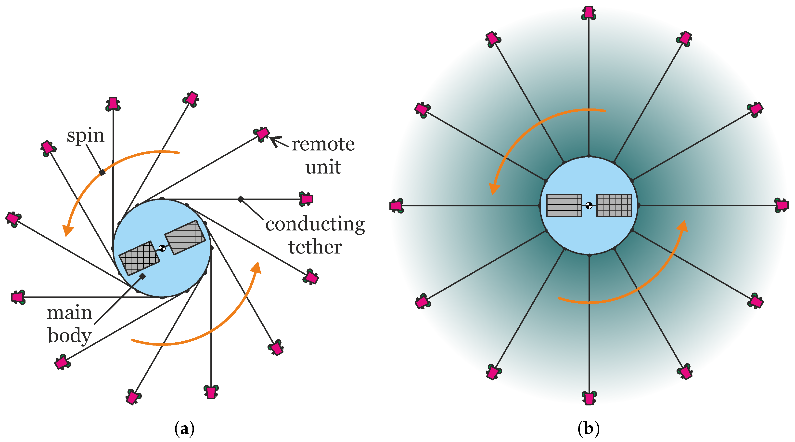
Figure 2.
Artistic impression of a CubeSat equipped with a spinning, single-tether E-sail, which can be used to obtain the first in situ measurement of the propulsive acceleration given by this fascinating propulsion system. In the artistic image, the CubeSat with a deployed (single) conducting tether covers a high-elliptic Lunar orbit which allows the vehicle to move outside Earth’s magnetosphere. Image courtesy of Mario F. Palos.
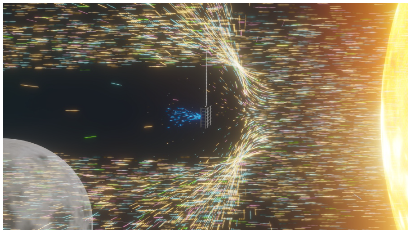
Figure 3.
Description of a Sun-facing configuration and a generic case in which the sail nominal plane is inclined with respect to the radial direction. (a) Sun-facing configuration in which the sail nominal plane is perpendicular to the Sun–spacecraft line; (b) case of a generic sail pitch angle different from zero, in which the E-sail-induced thrust vector has a non-zero transverse component.

Figure 4.
Radial-Transverse-Normal reference frame (RTN) of unit vector (radial), (transverse), and (normal). The plane coincides with the plane of the spacecraft osculating orbit, while the spacecraft inertial velocity vector has a positive component along the direction of .
Figure 4.
Radial-Transverse-Normal reference frame (RTN) of unit vector (radial), (transverse), and (normal). The plane coincides with the plane of the spacecraft osculating orbit, while the spacecraft inertial velocity vector has a positive component along the direction of .
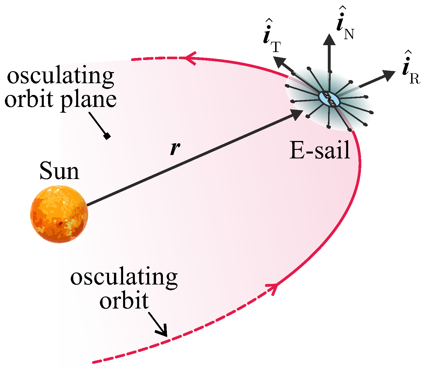
Figure 5.
Sketch of the normal unit vector and the propulsive acceleration vector in the RTN reference frame. The scheme introduces the sail pitch angle and the sail clock angle , which are the two (scalar) E-sail’s control terms.
Figure 5.
Sketch of the normal unit vector and the propulsive acceleration vector in the RTN reference frame. The scheme introduces the sail pitch angle and the sail clock angle , which are the two (scalar) E-sail’s control terms.

Figure 6.
Force bubble in the unconstrained case () when . The direction of propagation of the solar wind coincides with the direction of the z-axis, that is, the Sun belongs to the vertical axis.
Figure 6.
Force bubble in the unconstrained case () when . The direction of propagation of the solar wind coincides with the direction of the z-axis, that is, the Sun belongs to the vertical axis.

Figure 7.
Force bubble in the constrained case when and .
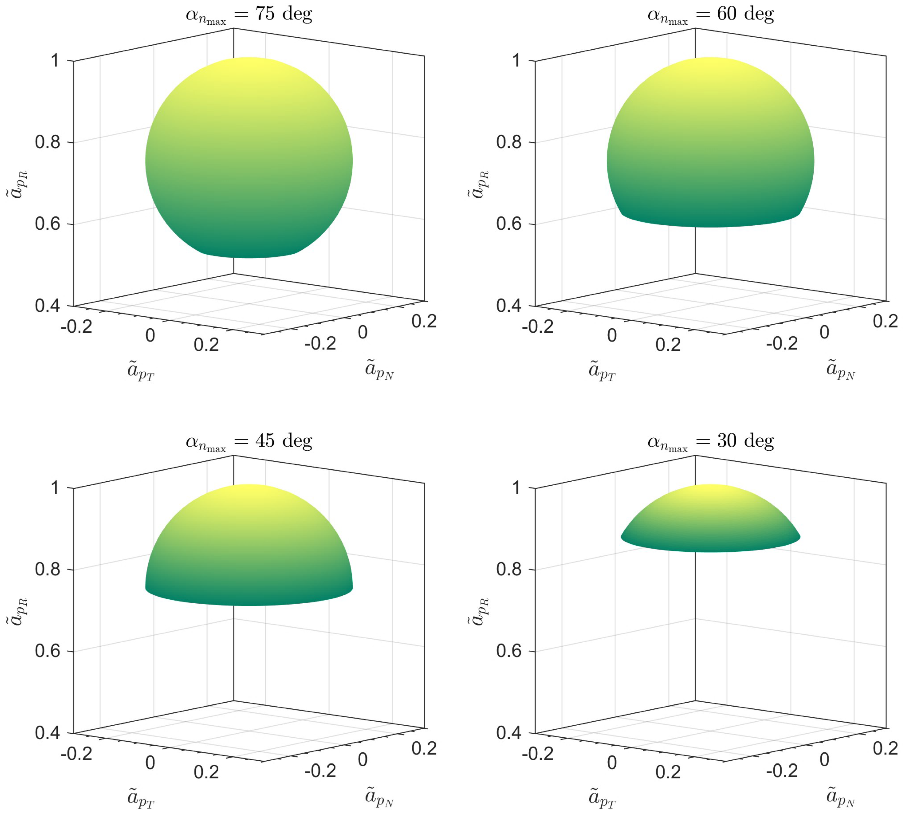
Figure 8.
Time variation in the control angles in an unconstrained Earth–Mars transfer with = 1 mm/s. Blue dot → starting point; red square → arrival point.
Figure 8.
Time variation in the control angles in an unconstrained Earth–Mars transfer with = 1 mm/s. Blue dot → starting point; red square → arrival point.
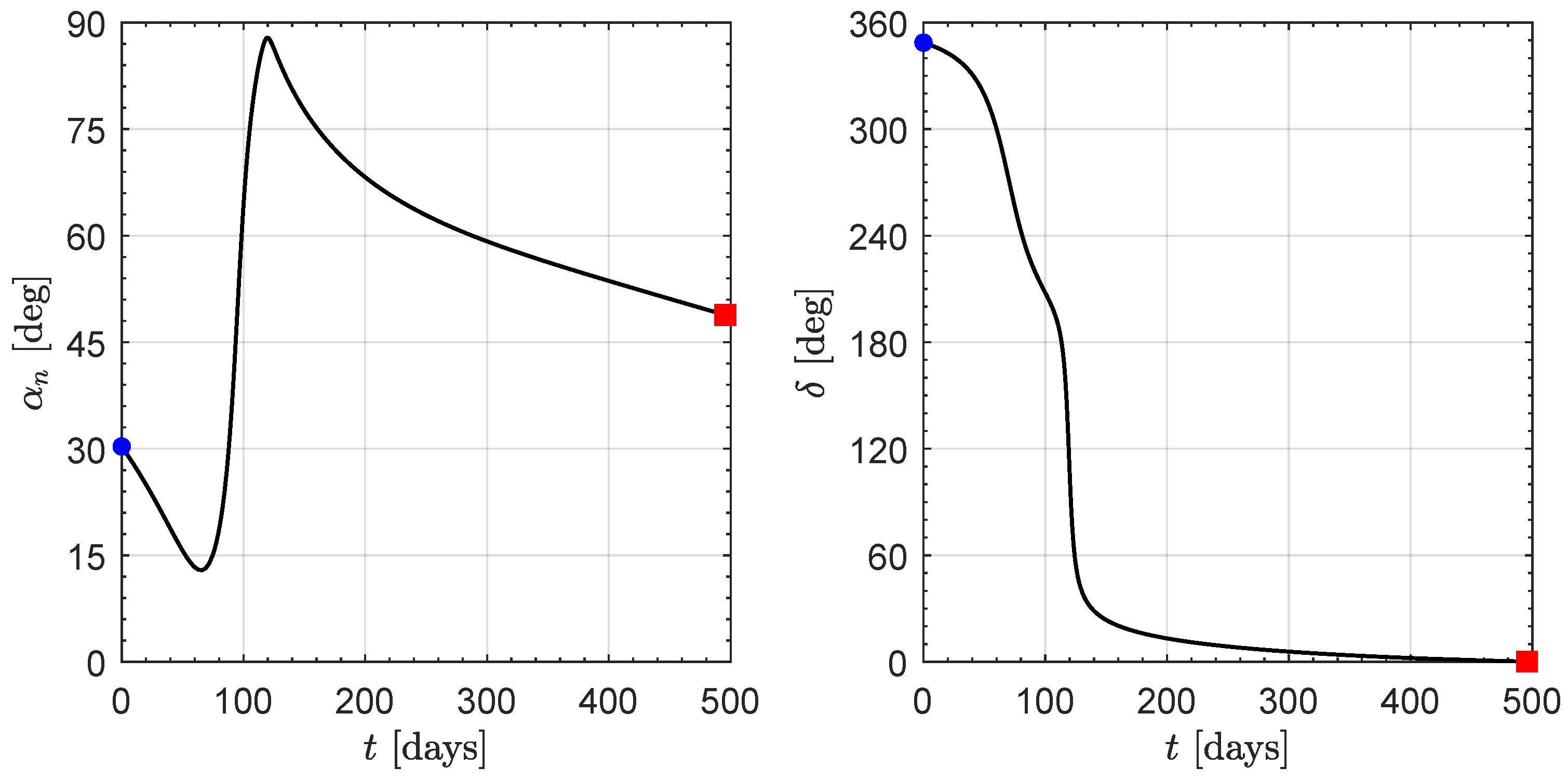
Figure 9.
Time variation in the control angles in an unconstrained Earth–Venus transfer with = 1 mm/s. Blue dot → starting point; red square → arrival point.
Figure 9.
Time variation in the control angles in an unconstrained Earth–Venus transfer with = 1 mm/s. Blue dot → starting point; red square → arrival point.
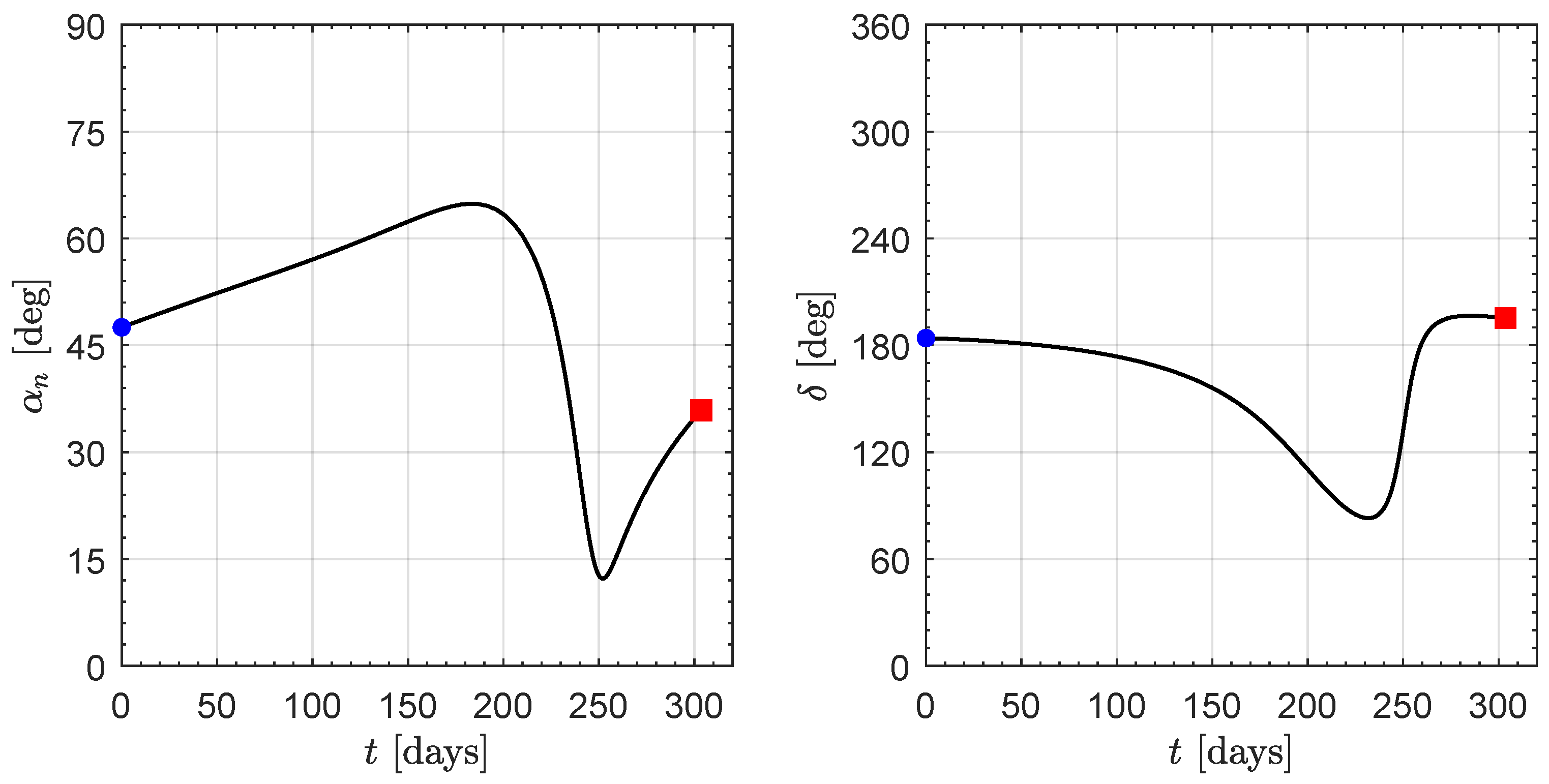
Figure 10.
Time variation in the control angles in an unconstrained Earth–Mercury transfer with = 1 mm/s. Blue dot → starting point; red square → arrival point.
Figure 10.
Time variation in the control angles in an unconstrained Earth–Mercury transfer with = 1 mm/s. Blue dot → starting point; red square → arrival point.
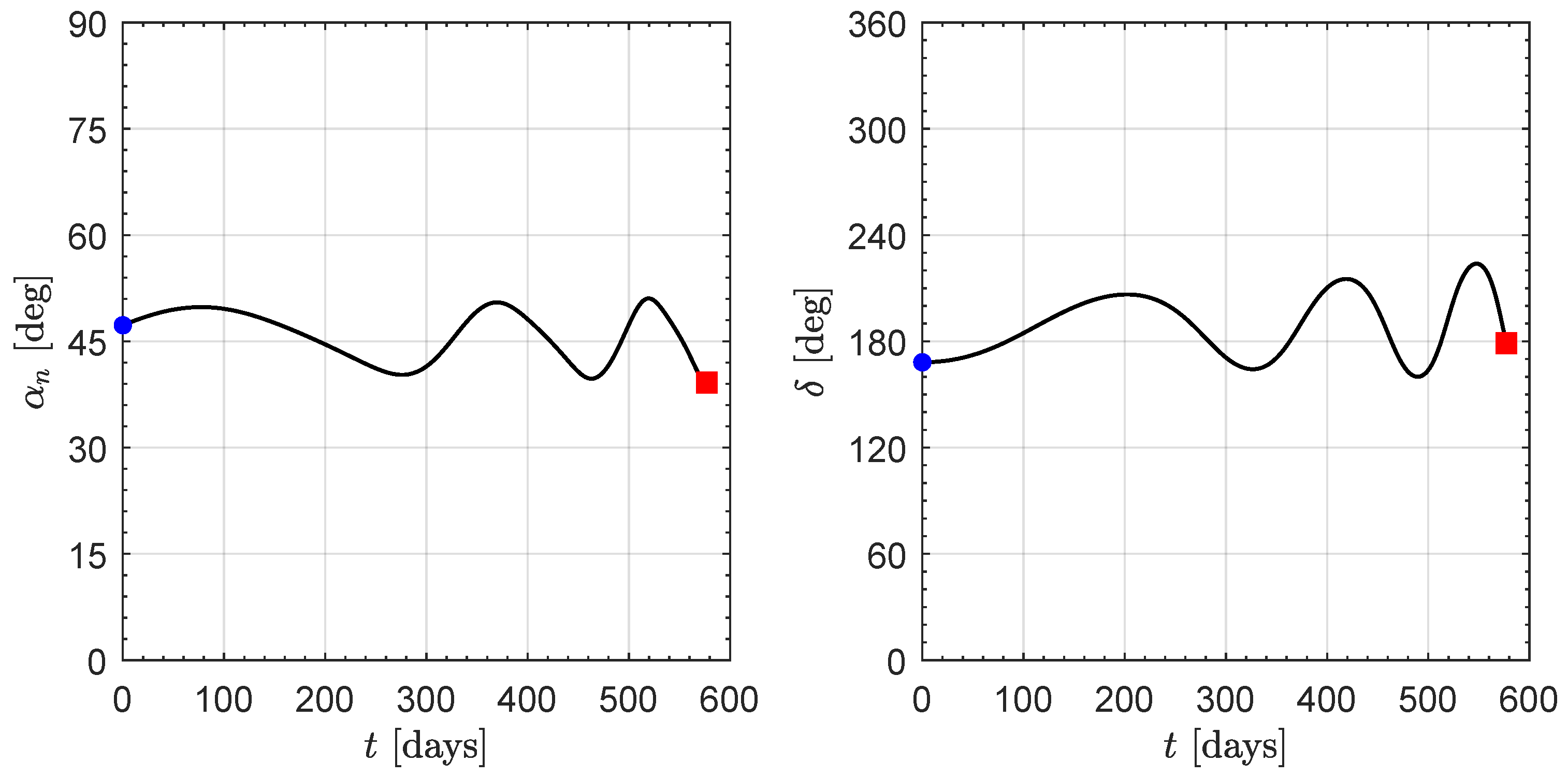
Figure 11.
Ecliptic projection and isometric view of the unconstrained optimal transfer trajectory in an Earth–Mars scenario with = 1 mm/s. Black line → optimal transfer trajectory; blue line → Earth’s orbit; red line → target planet’s orbit; filled star → planet’s perihelion; blue dot → starting point; red square → arrival point; orange dot → the Sun.
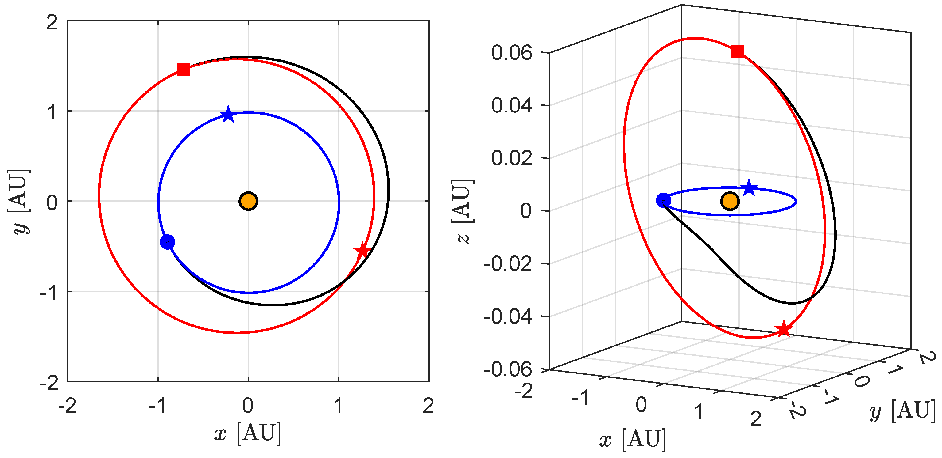
Figure 12.
Ecliptic projection and isometric view of the unconstrained optimal transfer trajectory in an Earth–Venus scenario with = 1 mm/s. See the caption of Figure 11 for the legend.
Figure 12.
Ecliptic projection and isometric view of the unconstrained optimal transfer trajectory in an Earth–Venus scenario with = 1 mm/s. See the caption of Figure 11 for the legend.
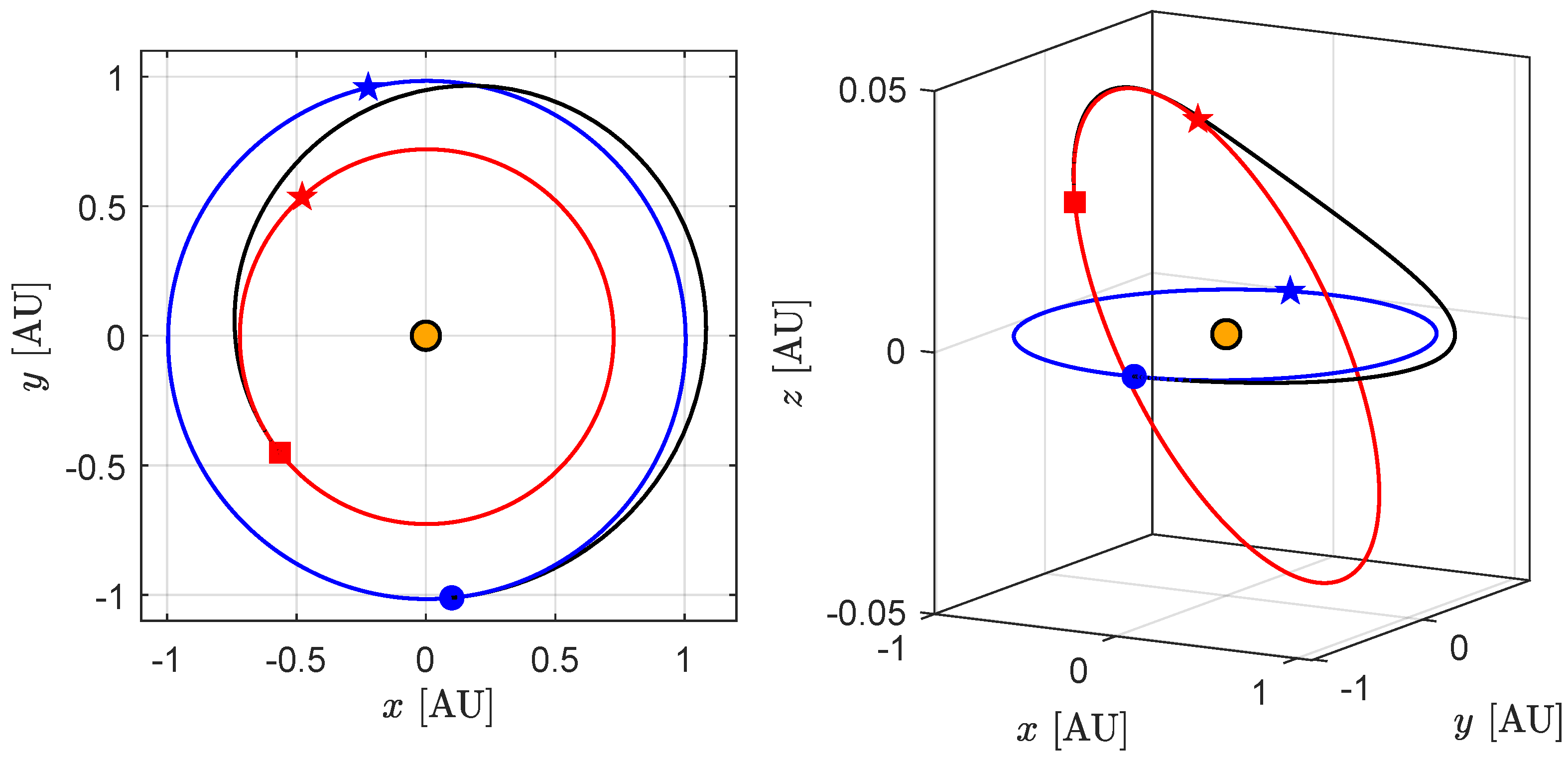
Figure 13.
Ecliptic projection and isometric view of the unconstrained optimal transfer trajectory in an Earth–Mercury scenario with = 1 mm/s. See the caption of Figure 11 for the legend.
Figure 13.
Ecliptic projection and isometric view of the unconstrained optimal transfer trajectory in an Earth–Mercury scenario with = 1 mm/s. See the caption of Figure 11 for the legend.
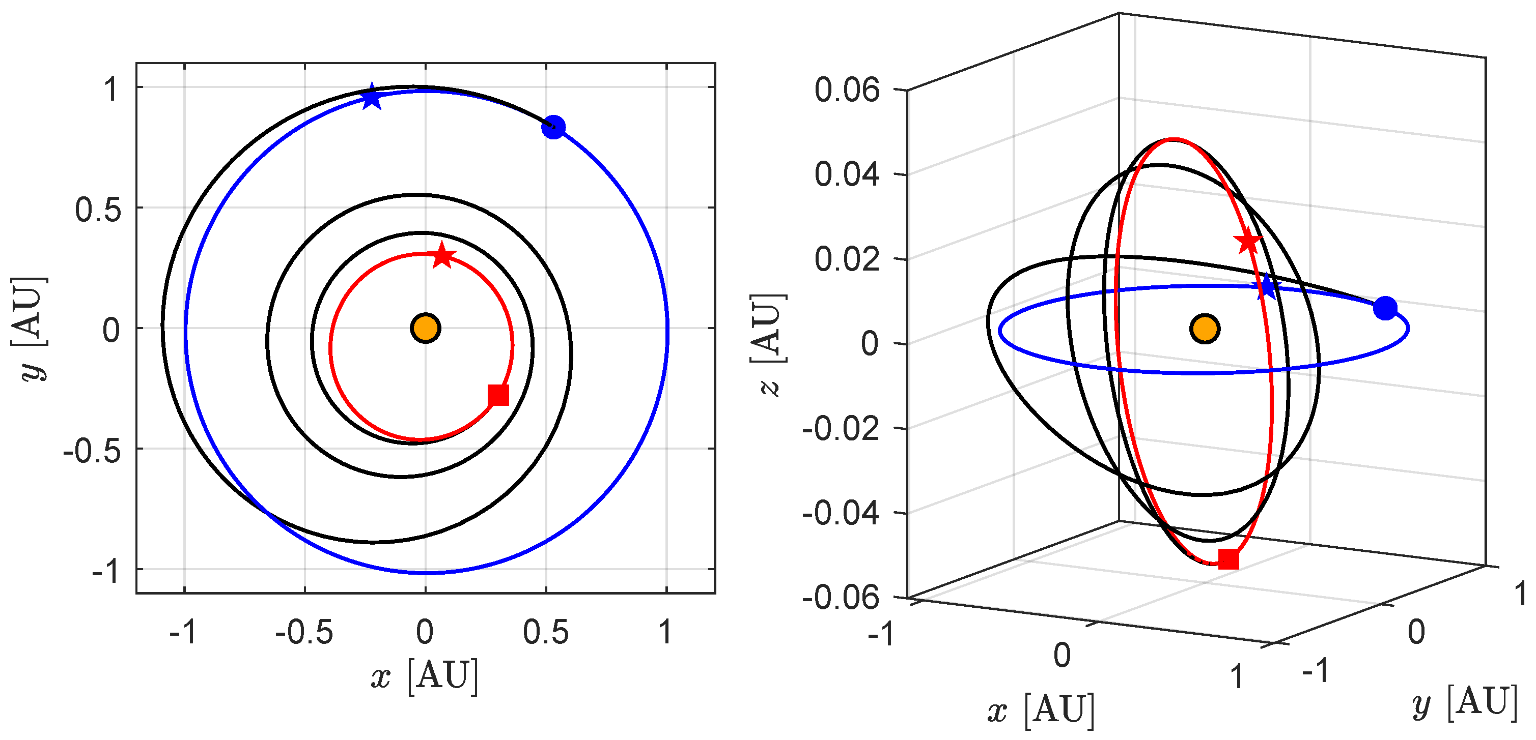
Figure 14.
Simulation results of the constrained case when = 1 mm/s. The dimensionless term D is defined in Equation (11). (a) Earth–Mars scenario; (b) Earth–Venus scenario; (c) Earth–Mercury scenario.
Figure 14.
Simulation results of the constrained case when = 1 mm/s. The dimensionless term D is defined in Equation (11). (a) Earth–Mars scenario; (b) Earth–Venus scenario; (c) Earth–Mercury scenario.

Figure 15.
Time variation in the control angles in a constrained Earth–Mars transfer with = 1 mm/s and . Blue dot → starting point; red square → arrival point.
Figure 15.
Time variation in the control angles in a constrained Earth–Mars transfer with = 1 mm/s and . Blue dot → starting point; red square → arrival point.
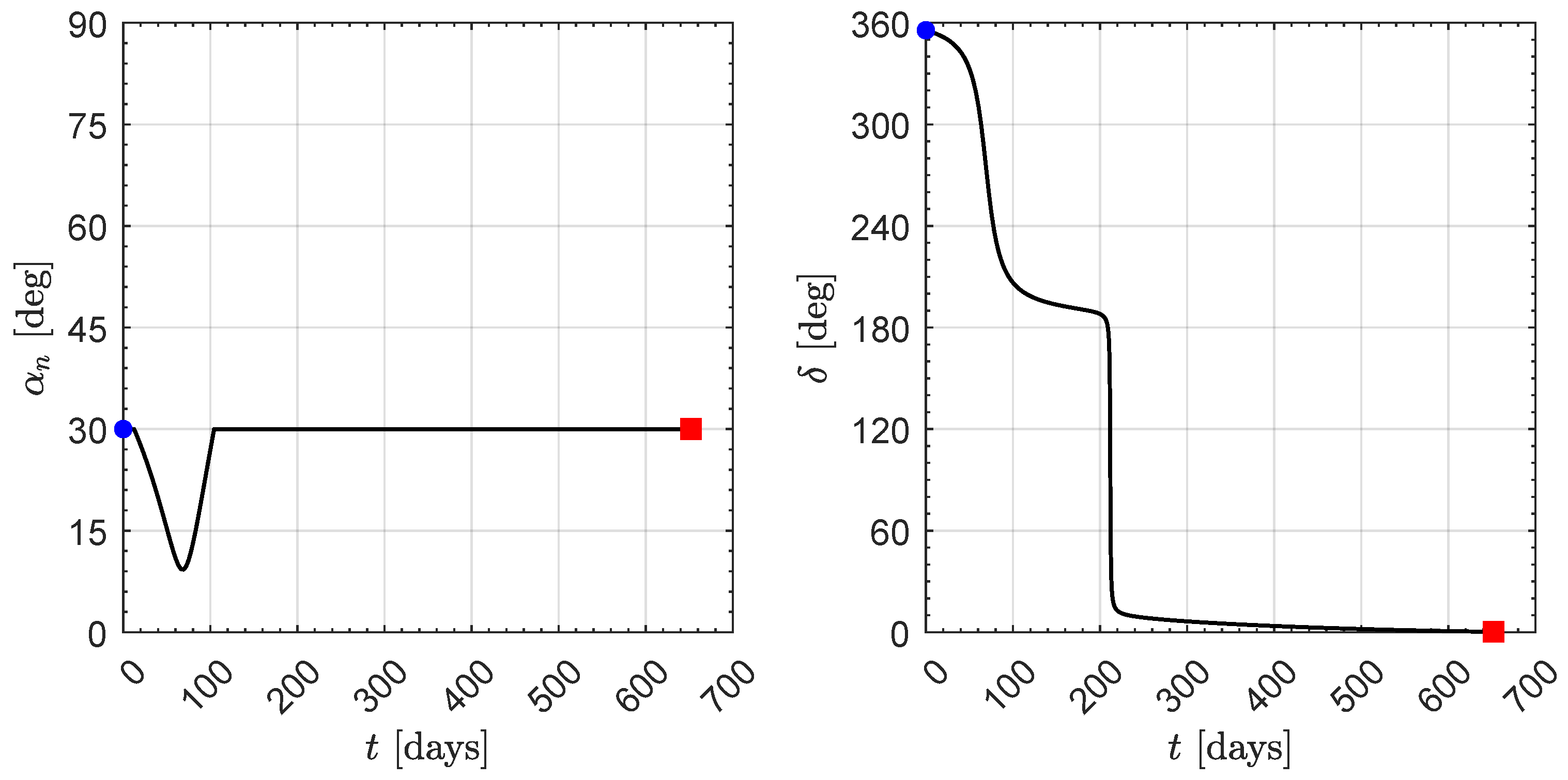
Figure 16.
Numerical results, in terms of minimum flight time , of the trajectory optimization in an Earth–Mars scenario, where and .
Figure 16.
Numerical results, in terms of minimum flight time , of the trajectory optimization in an Earth–Mars scenario, where and .

Figure 17.
Curve levels of the dimensionless parameter in an Earth–Mars scenario, where and .

Table 1.
Classical orbital elements of celestial bodies involved in interplanetary transfers analyzed in this section. The astronomical data were retrieved from the JPL Horizon system on 1 August 2024.
Table 1.
Classical orbital elements of celestial bodies involved in interplanetary transfers analyzed in this section. The astronomical data were retrieved from the JPL Horizon system on 1 August 2024.
| Planet | Semi-Major Axis | Eccentricity | Inclination | Argument of Perihelion | RAAN |
|---|---|---|---|---|---|
| Earth | |||||
| Mars | |||||
| Venus | |||||
| Mercury |
Table 2.
Simulation results for an unconstrained, three-dimensional, optimal orbit-to-orbit transfer when = 1 mm/s. The term is the minimum flight time, while [or ] is the maximum (or minimum) value of the sail pitch angle reached during the transfer. Recall that, by assumption, the propulsion system is always switched on during the flight, and the sail pitch angle is unconstrained.
| Scenario | |||
|---|---|---|---|
| Earth–Mars | |||
| Earth–Venus | |||
| Earth–Mercury |
Disclaimer/Publisher’s Note: The statements, opinions and data contained in all publications are solely those of the individual author(s) and contributor(s) and not of MDPI and/or the editor(s). MDPI and/or the editor(s) disclaim responsibility for any injury to people or property resulting from any ideas, methods, instructions or products referred to in the content. |
© 2024 by the author. Licensee MDPI, Basel, Switzerland. This article is an open access article distributed under the terms and conditions of the Creative Commons Attribution (CC BY) license (https://creativecommons.org/licenses/by/4.0/).
Share and Cite
MDPI and ACS Style
Quarta, A.A. Impact of Pitch Angle Limitation on E-Sail Interplanetary Transfers. Aerospace 2024, 11, 729. https://doi.org/10.3390/aerospace11090729
AMA Style
Quarta AA. Impact of Pitch Angle Limitation on E-Sail Interplanetary Transfers. Aerospace. 2024; 11(9):729. https://doi.org/10.3390/aerospace11090729
Chicago/Turabian StyleQuarta, Alessandro A. 2024. "Impact of Pitch Angle Limitation on E-Sail Interplanetary Transfers" Aerospace 11, no. 9: 729. https://doi.org/10.3390/aerospace11090729
Note that from the first issue of 2016, this journal uses article numbers instead of page numbers. See further details here.
Article Metrics
Article metric data becomes available approximately 24 hours after publication online.