A Zonal Detached Eddy Simulation of the Trailing Edge Stall Process of a LS0417 Airfoil

Abstract

A Zonal Detached Eddy Simulation (ZDES) based on the SST turbulence model is implemented to the numerical investigation of the trailing edge stall of a LS-0417 airfoil, which includes multiple DES modes for different classifications of flow separation and adopts the subgrid scale definition of ${\Delta }_{\omega }$. The entire stall process under a series of AOA is simulated according to the experiment condition. The performance of URANS and ZDES in the prediction of the stall flow field are compared. The results reveal that the stall point obtained through ZDES is consistent with the experiment; the deviation of the predicted maximum lift coefficient from the measured result is only 0.8%, while the maximum lift is overpredicted by both RANS and URANS. The high frequency fluctuations are observed in the time history of the lift in ZDES result during stall. With the increase in the AOA, a mild development of separation and a gradual decrease in leading edge peak suction are manifested in the ZDES result. The alternate shedding of shear layers and the interference between the leading edge and trailing edge vortices are illustrated through ZDES near the stall point; the corresponding turbulent fluctuations with high intensity are captured in the separation region, which indicates the essential difference in the prediction of stall process between URANS and ZDES.

1. Introduction

The trailing edge stall usually occurs on the airfoil with a relatively large thickness, which is characterized by the appearance of a separation point within the turbulent boundary layer and close to the trailing edge. The separation point moves towards the leading edge with the increase in the angle of attack (AOA) until the flow becomes massively separated. Compared with the leading edge separation or thin-airfoil separation, the change in the lift coefficient during the stall process is mild [1]; namely, the drop in the lift coefficient until full stall is very gradual and not sharp. Since the changes in separation location along the airfoil chord are driven by the pressure gradient, the precise prediction of the separation point movement is essential for the numerical simulation of this type of stall. Furthermore, under the stall process, the unsteady turbulent phenomena such as vortex generation and shedding will occur, which further enhance the difficulty of simulation. These characteristics bring a great challenge to the traditional Reynolds-Averaged Navier–Stokes (RANS) methods, especially in the prediction of stall points and shedding boundary layers [2].

In recent works, considering the simulation accuracy and efficiency of turbulence, DES (Detached Eddy Simulation)-type methods [3] are widely applied in the prediction of trailing edge stall or stall at large AOA. The capability of Large Eddy Simulation (LES) in the focus separation region and the feature of RANS in the attached boundary layers are integrated in the framework of DES-type methods. The NACA airfoils are usually chosen for the validation of DES. For the NACA 0012 airfoil, Shur [4] applied DES to the stall prediction at high AOA, Im [5] studied the stall through DDES (Delayed DES) [6] and DES, Yang [7] further carried out an IDDES (Improved DDES) [8] prediction of the stall and Wang [9] confirmed that the DES-type methods can satisfyingly simulate the nature fluctuations of stall. Furthermore, Gillings [10] used DES to simulate the trailing edge stall of the NACA0015 airfoil; the mildly separated flow was also investigated by Wang [11] with DES-type methods. Guo [12] numerically studied the flow around a NACA0018 airfoil at high incidences using RANS and DDES. DES was also used to analyze the aerodynamic characteristics of a NACA 633-018 airfoil by Li [13]. Moreover, other types of airfoils are also considered. Cokljat [14] conducted the simulation on the trailing edge separation of the A-airfoil with DES, and the performance of DES and DDES was compared by Durrani [15]. Low-Re separation flow around an NREL S826 blade profile was analyzed via DDES and SLA-DDES (Shear-Layer-Adapted DDES) [16] by Yalçın [17]. Compared with the URANS (Unsteady RANS), the results obtained with the DES-type methods are consistent with the experimental results in the statistics of stall features, while the description of the separation point and vortex behaviors are more precise.

However, for the traditional DES-type methods, the switch of the RANS and LES modes is based on the length scale which usually depends on the wall distance; then, in the so-called gray area [3] where the LES mode intrudes into the boundary layer, the undesirable phenomenon of modeled stress attenuation (MSD) and grid induced separation (GIS) might occur [6]. Though the delayed function in DDES protects the boundary layer from the LES mode, the excessive delay of the switch from RANS to LES is often observed in the simulation of mixing layers, which leads to the underprediction of the development of the shear layer instability. The flaw is mitigated in IDDES with a set of empirical formulas [8] while the modification of subgrid scales also contributes to the development of K-H instability [11]. But the complexity of method is also increased notably.

Another solution to eliminate the effects of gray area is to implement the ZDES [18]. The main idea of this method is to specify the RANS regions and the DES regions in the computational domain individually during simulation, so that the methods applied in each region are well defined and the gray area problem can be released to some extent. In addition, the approach allows multiple DES modes to operate in the same computational domain according to different separation types. Compared to the global DES-type methods, the approach provides more flexibility to the simulation. The capability of ZDES has been verified with the simulation of the unsteady turbulent flow around an OA209 airfoil [19] and a three-dimensional finite-span wing [20]. Furthermore, the hybrid length scale of ZDES provides the capability of simulating the second type II flow separation problem, where the separation is caused by the pressure gradient on a curved surface and the separation position is uncertain [18]. This feature of ZDES makes it appropriate for the prediction of a trailing edge stall.

In this paper, in order to the confirm the capability of ZDES in the prediction of a trailing edge stall, the numerical simulation on the stall process of a LS-0417 airfoil is performed with both URANS and ZDES, where the simulation is based on an in-house solver coupled with a finite volume method and multi-block structured grid. The calculation parameters are based on experimental conditions, with a Mach number of 0.15 for the incoming flow and a Reynolds number of 2.0 × 10⁶ based on the chord length c. The grid validation and the time step sensitivity analysis are carried out first. Then, the entire stall process under a series of AOA is simulated with the two methods. The performance in the prediction of flow field is comprehensively compared with both the time-averaged and the instantaneous results.

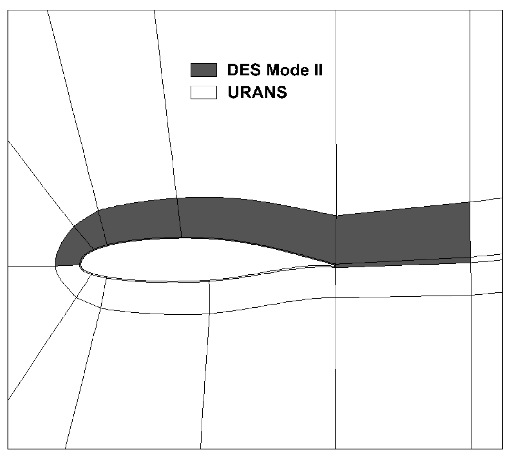
2. The Formulation of ZDES

2.1. The Definition of the Background Turbulence Model

The formulation of ZDES is based on the SST model of Menter [21], which is also the turbulence model employed in the URANS simulations. In the model, the conservation forms of the k equation and ω equation can be written as follows:

$${\displaystyle \frac{\mathsf{\partial }(\rho k)}{\mathsf{\partial }t}}+{\displaystyle \frac{\mathsf{\partial }(\rho u_{j}k)}{\mathsf{\partial }{x}_j}}=P-{\beta }^{*}\rho \omega k+{\displaystyle \frac{\mathsf{\partial }}{\mathsf{\partial }{x}_j}}\left((\mu +{\sigma }_k{\mu }_t){\displaystyle \frac{\mathsf{\partial }k}{\mathsf{\partial }{x}_j}}\right)$$

(1)

$$\begin{gathered} {\displaystyle \frac{\mathsf{\partial }(\rho \omega )}{\mathsf{\partial }t}}+{\displaystyle \frac{\mathsf{\partial }(\rho u_j\omega )}{\mathsf{\partial }{x}_j}}={\displaystyle \frac{\gamma }{{\nu }_t}}P-\beta \rho {\omega }^2+{\displaystyle \frac{\mathsf{\partial }}{\mathsf{\partial }{x}_j}}\left((\mu +{\sigma }_{\omega }{\mu }_t){\displaystyle \frac{\mathsf{\partial }\omega }{\mathsf{\partial }{x}_j}}\right) \\ +2(1-F_1){\displaystyle \frac{\rho {\sigma }_{\omega 2}}{\omega }}{\displaystyle \frac{\mathsf{\partial }k}{\mathsf{\partial }{x}_j}}{\displaystyle \frac{\mathsf{\partial }\omega }{\mathsf{\partial }{x}_j}} \end{gathered}$$

(2)

where ρ is the density, k is the turbulent kinetic energy, σ_k = 0.5, turbulent dynamic viscosity ${\nu }_t={\mu }_t/\rho$, μ is the molecular motion viscosity and d is the distance from the grid point to the wall.

The production term P can be written as follows:

$$P={\tau }_{ij}{\displaystyle \frac{\mathsf{\partial }{u}_i}{\mathsf{\partial }{x}_j}}$$

(3)

$${\tau }_{ij}={\mu }_t\left(2S_{ij}-{\displaystyle \frac{2}{3}}{\displaystyle \frac{\mathsf{\partial }{u}_k}{\mathsf{\partial }{x}_k}}{\delta }_{ij}\right)-{\displaystyle \frac{2}{3}}\rho k{\delta }_{ij}$$

(4)

$$S_{ij}={\displaystyle \frac{1}{2}}\left({\displaystyle \frac{\mathsf{\partial }{u}_i}{\mathsf{\partial }{x}_j}}+{\displaystyle \frac{\mathsf{\partial }{u}_j}{\mathsf{\partial }{x}_i}}\right)$$

(5)

The turbulent eddy viscosity coefficient μ_t is

$${\mu }_t={\displaystyle \frac{\rho a_{1}k}{\max (a_1\omega ,\Omega F_2)}}$$

(6)

The vorticity Ω is defined as follows:

$$\Omega =\sqrt{2W{ }_{ij}{W}_{ij}}$$

(7)

$$W_{ij}={\displaystyle \frac{1}{2}}\left({\displaystyle \frac{\mathsf{\partial }{u}_i}{\mathsf{\partial }{x}_j}}-{\displaystyle \frac{\mathsf{\partial }{u}_j}{\mathsf{\partial }{x}_i}}\right)$$

(8)

The parameters β, γ, σ_k and σ_ω can be written with ϕ:

$$\varphi =F_1{\varphi }_1+(1-F_1){\varphi }_2$$

(9)

where ϕ₁ and ϕ₂ represent the original coefficients of k-w model and the transformed model coefficients of k-ε model, respectively.

$$\left\{\begin{array}{l}{\gamma }_1={\displaystyle \frac{{\beta }_1}{{\beta }^{*}}}-{\displaystyle \frac{{\sigma }_{\omega 1}{\kappa }^2}{\sqrt{{\beta }^{*}}}}\\ {\sigma }_{k1}=0.85\\ {\sigma }_{\omega 1}=0.5\\ {\beta }_1=0.075\end{array}\right.$$

(10)

$$\left\{\begin{array}{l}{\gamma }_2={\displaystyle \frac{{\beta }_2}{{\beta }^{*}}}-{\displaystyle \frac{{\sigma }_{\omega 2}{\kappa }^2}{\sqrt{{\beta }^{*}}}}\\ {\sigma }_{k2}=1.0\\ {\sigma }_{\omega 2}=0.856\\ {\beta }_2=0.0828\end{array}\right.$$

(11)

where β* = 0.09, κ = 0.41, a₁ = 0.31.

The definitions of the hybrid functions F₁ and F₂ are as follows:

$$F_1=\tanh (ar{g}_1^4)$$

(12)

$$ar{g}_1=\min \left[\max \left({\displaystyle \frac{\sqrt{k}}{{\beta }^{*}\omega d}},{\displaystyle \frac{500\nu }{d^2\omega }}\right),{\displaystyle \frac{4\rho {\sigma }_{\omega 2}k}{C{D}_{k\omega }{d}^2}}\right]$$

(13)

$$C{D}_{k\omega }=\max \left({\displaystyle \frac{2\rho {\sigma }_{\omega 2}}{\omega }}{\displaystyle \frac{\mathsf{\partial }k}{\mathsf{\partial }{x}_j}}{\displaystyle \frac{\mathsf{\partial }\omega }{\mathsf{\partial }{x}_j}},{10}^{-20}\right)$$

(14)

$$F_2=\tanh (ar{g}_2^2)$$

(15)

$$ar{g}_2=\max \left(2{\displaystyle \frac{\sqrt{k}}{{\beta }^{*}\omega d}},{\displaystyle \frac{500\nu }{d^2\omega }}\right)$$

(16)

2.2. The Definition of the Hybrid Length Scale

Similar to the typical DES method, ZDES also requires the modifications of the destruction term in the turbulence model. After introducing the length scale of ${\tilde{l}}_{\mathrm{ZDES}}$, the transport equation of turbulent kinetic energy can be rewritten as follows:

$${\displaystyle \frac{\mathsf{\partial }(\rho k)}{\mathsf{\partial }t}}+{\displaystyle \frac{\mathsf{\partial }(\rho u_{j}k)}{\mathsf{\partial }{x}_j}}={\tau }_{ij}{\displaystyle \frac{\mathsf{\partial }{u}_i}{\mathsf{\partial }{x}_j}}-{\displaystyle \frac{\rho k^{3/2}}{{\tilde{l}}_{\mathrm{ZDES}}}}+{\displaystyle \frac{\mathsf{\partial }}{\mathsf{\partial }{x}_j}}\left((\mu +{\sigma }_k{\mu }_t){\displaystyle \frac{\mathsf{\partial }k}{\mathsf{\partial }{x}_j}}\right)$$

(17)

For the original SST turbulence model, the length scale values are set as follows:

$${\tilde{l}}_{\mathrm{ZDES}}=l_{\mathrm{SST}}={\displaystyle \frac{\sqrt{k}}{{\beta }^{*}\omega }}$$

(18)

For the global DES-type method, the RANS and the LES regions are determined through a hybrid function; however, the regions of RANS and DES can be specified independently as demanded in ZDES; namely, the different mixing length scales are defined based on the types of separated flow in the focus region, while RANS is applied in other regions [18].

In this paper, ZDES is realized under the structured multi-block grid, hence, with the definition of a parameter $ide{s}_n$ on the special block, the allocation of RANS/DES in corresponding regions of the computational domains can be specified as follows.

In a computational domain composed of N blocks, for the nth grid block (0 < n < N), when $ide{s}_n=0$, RANS is used in that region; when $ide{s}_n=1$, DES is used in that region. Thus, the hybrid length scale can be defined as follows:

$${\tilde{l}}_{ZDES}=(1-ide{s}_n)\times l_{RANS}+ide{s}_n\times l_{DES}^{\mathrm{I} \mathrm{or} \mathrm{II}}$$

(19)

The selection of $l_{DES}^{I or II}$ is specified through $imode$. When $imode=1$, it corresponds to the flow separation of type I. When $imode=2$, it corresponds to the type II.

$${\tilde{l}}_{\mathrm{ZDES},\mathrm{n}}=\left\{\begin{array}{l}{l}_{\mathrm{SST}},\mathrm{for} ide{s}_n=0\\ l_{\mathrm{DES}}^{\mathrm{I}},\mathrm{for} ide{s}_n=1_{ }\mathrm{and} imod{e}_n=1\\ l_{\mathrm{DES}}^{\mathrm{II}},\mathrm{for} ide{s}_n=1_{ }\mathrm{and} imod{e}_n=2\end{array}\right.$$

(20)

When $ide{s}_n=1$ and $imode=1$, the region corresponds to flow I.

$${\tilde{l}}_{\mathrm{ZDES},n}=l_{\mathrm{DES}}^{\mathrm{I}}=\min (l_{SST},C_{\mathrm{DES}}\Delta )$$

(21)

When $ide{s}_n=1$ and $imode=2$, the region corresponds to flow II.

$${\tilde{l}}_{\mathrm{ZDES},n}=l_{\mathrm{DES}}^{\mathrm{II}}=l_{\mathrm{SST}}-f_d\max (0,l_{\mathrm{SST}}-C_{\mathrm{DES}}\Delta )$$

(22)

The above two equations are similar to the original DES97 and DDES in terms of composition, while ZDES adopts a new subgrid scale Δ.

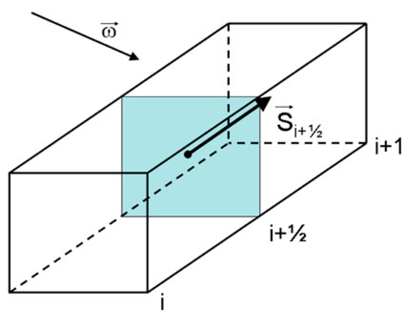
2.3. The Definition of the Subgrid Scale

To address the problem of traditional DES-type methods where the activation of LES mode is usually delayed in the resolving of mixing layer, Chauvent [22] proposed a new subgrid scale, which can be defined as follows:

$$\Delta ={\Delta }_{\omega }=\sqrt{{\overline{S}}_{\omega }}$$

(23)

where ${\overline{S}}_{\omega }$ is the specified cross-section area, the normal vector of the section is defined as the rotation axis of a local vortex.

For a cell of the structured grid in Figure 1, if $s_i$ and $s_{i+1}$ represent the areas of i and i + 1, respectively, the area of interface i + 1/2 can be defined as follows:

$$s_{i+1/2}={\displaystyle \frac{1}{2}}(s_i+s_{i+1})$$

(24)

The component of the unit vector of the rotation axis N of the vorticity $\omega$ in the i direction is

$$N_i={\displaystyle \frac{\left(\mathit{\omega }.\mathbf{i}\right)}{‖\mathit{\omega }‖}}$$

(25)

To avoid numerical errors, the equation is usually written in the following form:

$$\mathbf{N}={\displaystyle \frac{\mathit{\omega }+\mathbf{\epsilon }}{‖\mathit{\omega }+\mathbf{\epsilon }‖}}$$

(26)

$$\mathit{\epsilon }={\displaystyle \frac{\epsilon }{\sqrt{3}}}\left(\mathbf{i}+\mathbf{j}+\mathbf{k}\right)$$

(27)

Here, ε is a small quantity, which is usually taken as $\epsilon ={10}^{-8}$.

For the cell-centered finite volume method with structured grid, ${\Delta }_{\omega }$ can be written as follows:

$${\Delta }_{\omega }=\sqrt{{\overline{S}}_{\omega }}=\sqrt{{\displaystyle \frac{{‖N_i‖}^2}{s_{j+1/2}{s}_{k+1/2}}}+{\displaystyle \frac{{‖N_j‖}^2}{s_{k+1/2}{s}_{i+1/2}}}+{\displaystyle \frac{{‖N_k‖}^2}{s_{i+1/2}{s}_{j+1/2}}}}$$

(28)

For the length scale $l_{DES}^{II}$ corresponding to the type II flow separation, in order to ensure that the RANS mode can quickly switch to LES mode in the focus region, the delay function $f_d$ is applied. The value $f_{d0}$ is introduced to mark the outer edge of the boundary layer, which can be written as the following form:

$${\Delta }_{\mathrm{DES}}^{\mathrm{II}}=\left\{\begin{array}{l}{\Delta }_{\max }, \mathrm{if} f_d<f_{d0}\\ {\Delta }_{\omega }, \mathrm{if} f_d>f_{d0}\end{array}\right.$$

(29)

Here, the range of $f_{d0}$ is (0.75, 0.99). The minimum value of $f_{d0}$ is aimed at maintaining the original DDES behavior within the boundary layer, while the maximum value corresponds to the subgrid length scale ${\Delta }_{max}$. Therefore, as long as $f_d<f_{d0}$, the equation remains in DDES mode.

In summary, the subgrid scale of ZDES is defined as follows:

For the type I flow separation problem, where the separation positions are fixed, the subgrid length scale is

$${\Delta }_{\mathrm{DES}}^{\mathrm{I}}={\Delta }_{\mathsf{\omega }}$$

(30)

For the type II flow separation problem, where the separation positions are uncertain, the subgrid length scale is

$${\Delta }_{\mathrm{DES}}^{\mathrm{I}}=(0.5+\mathrm{sign}(0.5,f_d-f_{d0}))\times {\Delta }_{\max }+(0.5-\mathrm{sign}(0.5,f_d-f_{d0}))\times {\Delta }_{\mathsf{\omega }}$$

(31)

The sign function is defined as

$$\mathrm{sign}(a,b)=\left\{\begin{array}{l}+a,\mathrm{if} b\ge 0\\ -a,\mathrm{if} b<0\end{array}\right.$$

(32)

In the paper, ZDES is integrated in an in-house solver coupled with a finite volume method and multi-block structured grid; the DES capability of the code has been verified with a series of cases [23,24,25]. The fifth-order Roe-WENO scheme [26] is applied to enhance the resolution of spatial flow structures.

3. The Prediction of Stall

3.1. The Introduction of the Airfoil and the Experiment

The low-speed airfoil LS-0417 [27] is selected for the simulation with both URANS and ZDES. LS-0417 is a airfoil designed by NASA, with a design lift coefficient of 0.4 and a relative thickness of 17%. The airfoil is characterized by a curved upper surface, a flat lower surface and a large aft camber.

The aerodynamic forces were measured in the NASA Langley low-turbulence wind tunnel [28]. The tunnel is a closed-throat single return tunnel which can be operated at stagnation pressures ranging from 1 to 10 atm with tunnel-empty test-section Mach numbers up to 0.46 and 0.23, respectively. The maximum unit Reynolds number is about 49 × 10⁶ per meter at the Mach number of 0.23. The test section is 91.44 cm wide by 228.6 cm high. The airfoil model was machined from a solid aluminum billet and had a chord of 58.42 cm and a span of 91.44 cm to span the wind tunnel completely. The two-dimensional airfoil was attached through a two-component force balance at each end to circular end plates. The model was mounted with the quarter chord coincident with the rotational axis of the circular plates. The results were compared with a three-dimensional wind-tunnel and flight data. The lift-curve slopes of the corrected two-dimensional data were in good agreement with the lift-curve slopes obtained from the three-dimensional wind-tunnel and flight data [29]. The calculation conditions are based on the experiment, with a Mach number of 0.15 for the incoming flow and a Reynolds number of 2.0 × 10⁶ based on the chord length c.

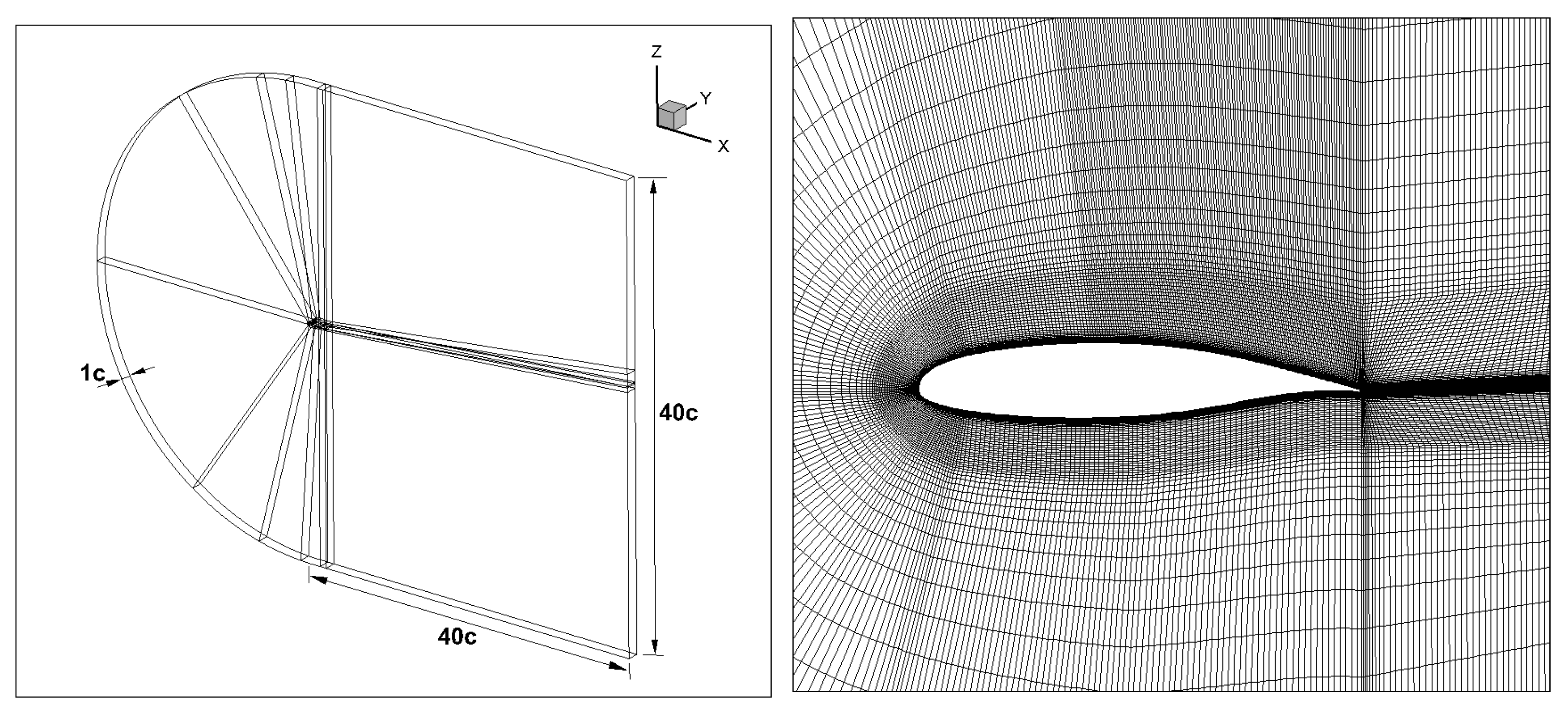
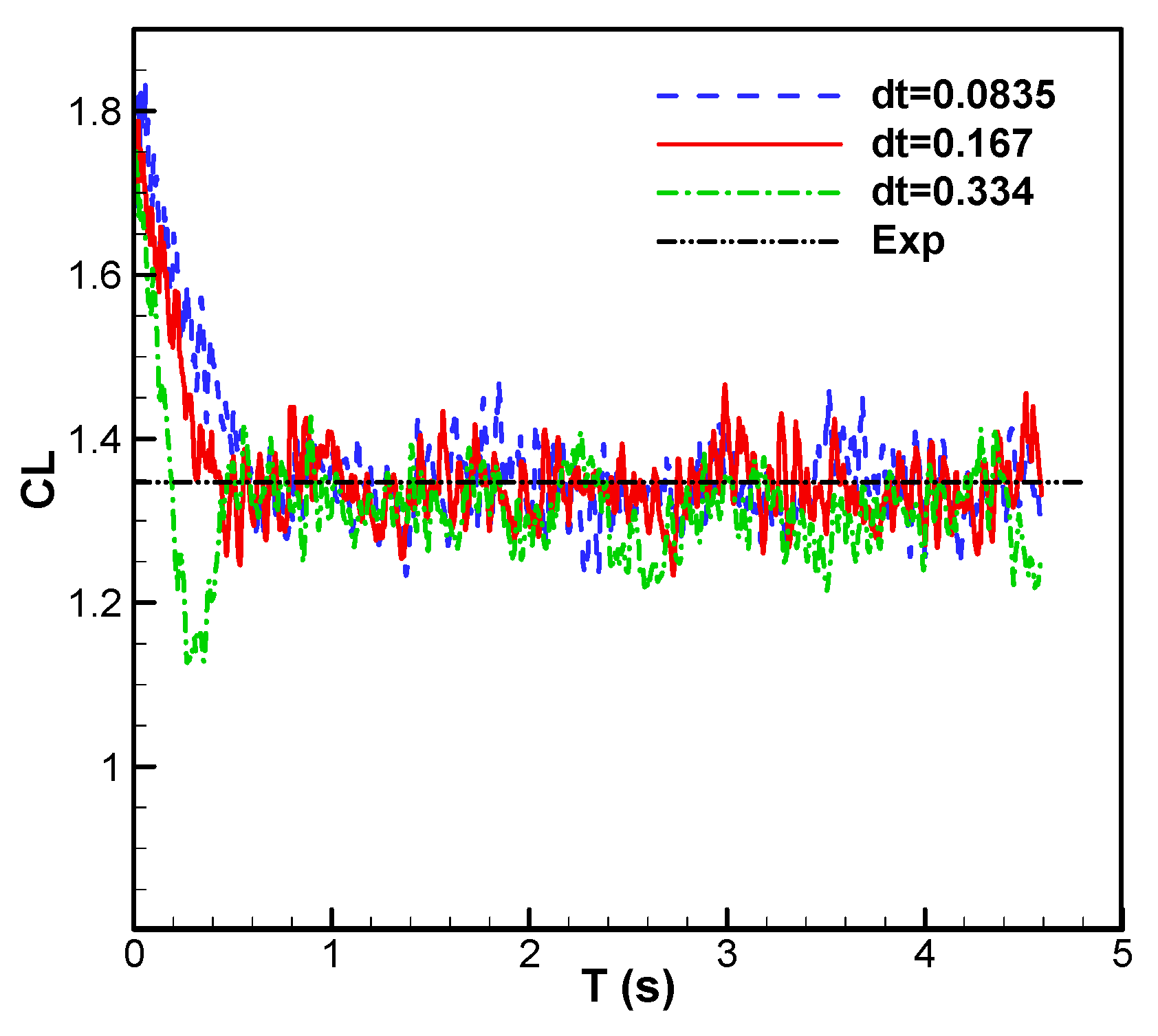
3.2. The Grid Density and the Time Step Validation

The muti-block structured computational grid adopts a C-type topology, which is shown in Figure 2. The length of upstream far-field is set as 20c and the length of downstream far-field of the airfoil is set as 40c. According to the suggestion of Shur [4], setting the spanwise length of the computation domain as one chord can capture the typical separation structures, which is sufficient for simulating the stall at high AOA. To study the influence of grid scale on the numerical results, two sets of computational grids are generated based on the same topology. The total number of grid points in coarse grid (Mesh-C) is $0.91\times {10}^6$ and in fine grid (Mesh-F) is $2.1\times {10}^6$. The corresponding distribution of grid nodes is shown in

Table 1. Nodes distribution of different computational grid.

	Chordwise	$\mathbf{Max} \Delta {\mathit{x}}^{+}$	Normal	${\mathit{y}}^{+}$	Spanwise	$\mathbf{Max} \Delta {\mathit{z}}^{+}$
Mesh-C	281	400	87	0.8	29	3000
Mech-F	332	300	121	0.8	41	2000

, since with the application of C-H topology, the number of grid points only indicates the cells around the airfoil; the points in the wake region are not included. The comparison of the grid numbers and sizes of several other similar studies is provided in

Table 2. Grid size of different DES simulation of trailing edge stall or post-stall problem.

Airfoil	DES-Type Methods	Re	AOA	Grid Size
NACA0012 [4]	DES	1 × 105	45°	2.0 × 105
NACA0012 [5]	DES and DDES	1.3 × 106	17°/25°/ 45°/60°	6.0 × 105
NACA0012 [7]	IDDES	1.3 × 106	5°/17°/ 45°/60°	8.64 × 105
NACA0012 [9]	IDDES	1.3 × 106	45°	5.87 × 105
NACA0015 [10]	DES	1.6 × 106	12°~20°	2.0 × 107
NACA0015 [11]	DDES and IDDES	1.0 × 106	11°	1.35 × 107
NACA0018 [12]	DDES	1.0 × 106	5°~40°	2.07 × 106
NACA633-018 [13]	DES	5.8 × 106	0°~18°	4.07 × 105
A-airfoil [14]	DES	2.1 × 106	13.3°	3.78 × 105
A-airfoil [15]	DES and DDES	2.0 × 106	13.3°	2.00 × 106
NREL S826 [17]	SLA-IDDES	1.0 × 106 and 1.45 × 106	4°~12°	9.47 × 105

, indicating that the frequently used order of grid size for the airfoil stall problem is ${10}^6$ or lower. The grid size near the airfoil of current study is similar to the works of Yang [7]. The normal distance of the first layer of the grid near the wall of both sets of the grid is defined as $1\times {10}^{-5}c$ to ensure $y^{+}<1$. Inflow/outflow boundary conditions are used for the far-field; the no-slip conditions are for the wall and there are symmetries conditions are for the two sides.

Both URANS and ZDES are adopted in the analysis of grid scale effects. The physical time step of unsteady calculation is chosen as $2.89\times {10}^{-4}$s, which is equivalent to a 2.5% chord length flow period; a chord length flow period is defined as the time taken for a particle to travel from the leading edge to the trailing edge. The corresponding flow courant numbers are about 7.1 for the coarse grid and 8.4 for the fine grid with the current time step adaptation. Shur [4] suggests that a complete case of airfoil separation simulation should include at least 100~200 chord length periods. Considering the convergence process of unsteady calculation in the initial state, a total of 16,000 time steps were calculated, which is equal to 400 chord length periods, where 10 pseudo iterations were involved in each time step. To ensure the accuracy of the statistical average results, the last 350 chord length convection periods (including at least 14,000 time steps) were taken for time averaging.

The definition of the calculation region of ZDES is shown in Figure 3. The DES mode of the type II flow separation is applied over the dark regions on the upper surface of the airfoil, which is divided by the edges of blocks, while the RANS mode is used in the other regions. Considering the streamwise evolution of separated flow, the length of the wake region is selected as approximately 80% c, where DES mode is also activated.

According to the experimental results, the stall AOA of the LS0417 airfoil is approximately ${16}^{°}$ at $Re=2.1\times {10}^6$. The condition for the grid validation is chosen as the post-stall at $\alpha ={18}^{°}$. The convergence history of the lift coefficient is provided in Figure 4. It is indicated that the aerodynamic coefficients obtained through URANS are periodic and regular, while the ZDES result exhibits obvious features of unsteadiness; the high frequency fluctuations of lift are observed in the time history. The time-averaged lift coefficients are listed in

Table 3. Lift coefficient predicted with different computational grid and method.

	URANS	ZDES	Exp
Mesh-C	0.9684	1.3197	1.35
Mech-F	0.9826	1.3398

. Comparing the results obtained with different methods, the lift coefficient is notably underpredicted by URANS and the divergence of the coarse and fine grid from the experimental value reaches to −28.3% and −27.2%, respectively. The time-averaged lift coefficients obtained using ZDES are basically consistent with the measured results and the corresponding divergences of the two sets of grids are only −2.24% and −0.76%. Comparing the results obtained with the different grid, the divergence due to the resolution of the grid is not significant; the time-averaged lift coefficients on the coarse grid predicted by URANS and ZDES are 1.45% and 1.50% lower than those on the fine grid, respectively. The result indicates that the current computational grid has a convergence to some degree; in the subsequent simulation, the fine grid (Mesh-F) is implemented.

In order to study the sensitivity of numerical results to the time step, the numerical simulation of ZDES is carried out with different physical time steps, which are $1.445\times {10}^{-4} \mathrm{s}, 2.89\times {10}^{-4} \mathrm{s}$ and $5.78\times {10}^{-4} \mathrm{s};$ the corresponding dimensionless time steps are $\Delta t=0.08375, 0.167 \mathrm{and} 0.33$, respectively. The convergence history of the lift coefficients with different time steps are given in Figure 5. The time-averaged result is shown in

Table 4. Time-averaged lift coefficients predicted with different time steps.

dt	0.334	0.167	0.0835	Exp
CL	1.3121	1.3398	1.3418	1.35

. It can be seen that the difference in the result with the three selected time steps is small, but when the length of the time step is reduced, the consistency of the numerical result with the measured data is better. In the subsequent simulation, the non-dimensional time step of $\Delta t=0.167$ is selected in the consideration of accuracy and efficiency.

3.3. The Prediction of Stall Process

In this section, the performance of URANS and ZDES are further compared to perform the simulation of a complete lift line from $\alpha =-{10}^{°}$ to $\alpha ={22}^{°}$. Figure 6 and

Table 5. Comparison of $\mathrm{CL}$ obtained with different methods.

AOA	CL of EXP	URANS		ZDES
		CAL	ERR	CAL	ERR
12	1.48	1.5987	8.02%	1.5527	4.91%
14	1.57	1.671	6.43%	1.5726	0.17%
16	1.59	1.5345	−3.49%	1.5773	−0.80%
18	1.35	0.9826	−27.21%	1.3398	−0.76%

illustrate the result of lift coefficients obtained with different methods. All the numerical results are basically consistent at low AOA before $\alpha =4^{°}$, which is in good agreement with the experimental results [27]. However, as the AOA increases, the numerical results demonstrate more linearity compared with the experiment until the stall point. The stall AOA and maximum lift coefficient are both overpredicted notably by RANS, while the maximum lift coefficient predicted by URANS is also higher than the experimental value, but the accuracy of stall AOA capturing is improved. The stall point predicted by ZDES is basically consistent with the experiment, with the maximum lift coefficient appearing at $\alpha ={16}^{°}$ and the deviation of magnitude is only 0.8%. Furthermore, ZDES can also obtain lift coefficients consistent with experimental results under post-stall condition ($\alpha ={18}^{°}$ and $\alpha ={20}^{°}$), but a sharper decrease in lift is obtained using RANS and URANS. It is noticed that all results overpredict the lift coefficient between $\alpha =5^{°}~{15}^{°}$; a reasonable explanation can be given, where that due to the initial trailing separation occurring under the $\alpha =5^{°}$, there is a slight degeneration of lift coefficient. However, since the separation area is negligible compared with the chord length (less than 5% of the chord) according to the result of experiment [27], the current methods fail to predict this subtle flow phenomenon.

Figure 7 compares the convergence history of the lift coefficient obtained through URANS and ZDES at four different AOAs. At the pre-stall condition of $\alpha =8^{°}$, the time-averaged lift coefficient predicted with URANS is basically consistent with ZDES, both of which are slightly higher than the experimental values. The notable fluctuation of the lift coefficient is not observed in the time history, indicating that the unsteadiness of the flow is not apparent. At the stall point of $\alpha ={16}^{°},$ the regular fluctuation of the lift coefficient can be observed in the ZDES result, while the fluctuation predicted by URANS is still not significant. At the post-stall point of $\alpha ={18}^{°}$, both the URANS and ZDES results exhibit noticeable fluctuation, but the URANS result is more regular with only the main peak of fluctuation predicted, while the secondary fluctuation can be captured by ZDES. It is noteworthy that at $\alpha ={20}^{°}$, the fluctuation predicted by RANS is degenerated significantly, which contradicts the massive, separated flow nature of the post-stall condition. Overall, the unsteady characteristics of the lift coefficients during the stall process in the ZDES result are more pronounced than those in URANS.

Figure 8 gives the time-averaged streamline obtained using URANS and ZDES under the stall process. For $\alpha ={14}^{°}$, at the point of maximum lift coefficient predicted by URANS, the corresponding distribution of the streamline shows that a recognizable separation region has generated at the trailing edge of the airfoil, but the local separation tendency predicted by ZDES is negligible. The maximum lift point predicted by ZDES is at $\alpha ={16}^{°}$; both the range and the height of separation region are almost unchanged. However, the separation region increases notably in the URANS result. At the post-stall condition of $\alpha ={18}^{°}$, a massive separated flow region generates in the URANS result, which is characterized with the significant forward movement of the initiation point of the separation region and the increase in the main vortex height, corresponding to the sharp decrease in lift under the post-stall condition. By contrast, the growth of the separation region of ZDES is gradual. At the larger AOAs, the separation region predicted by URANS is still larger than ZDES. In general, with the increase in the AOA, the expanding tendency of the separation region at the trailing edge during the stall process is both predicted by URANS and ZDES, but overall, a more gradual growth in the size of the recirculation region and the height of the vortex core are manifested in the ZDES result.

The time-averaged pressure distributions at different AOAs obtained through URANS and ZDES during the stall process are given in Figure 9. At $\alpha ={16}^{°}$, since the separation region is limited near the trailing edge of the airfoil, no major difference is observed in the pressure distribution of the two methods. At $\alpha ={18}^{°}$, the peak suction at the leading edge obtained with URANS is much lower than that of ZDES, and the following pressure platform is extended, which indicates a large-scale separation region. The result also shows that the initial location of separation predicted by ZDES occurs approximately at x/c = 45%, while the location predicted by URANS is advanced to x/c = 25%. At larger AOAs of post-stall conditions, the gradual decrease in peak suction can still be obtained using ZDES, which corresponds to a more reasonable separation evolution.

Figure 10 shows the comparison of instantaneous vorticity distribution obtained with URANS and ZDES. In general, though the main shedding layers are identified by URANS, the secondary turbulent structures fail to be captured. At $\alpha ={16}^{°}$, the topology of separation is similar for the two methods, but at $\alpha ={18}^{°}$, the shedding point of the boundary layer predicted by URANS is closer to the leading edge and the shedding angle of the boundary layers is abnormally large, while the shedding point predicted by ZDES is at the mid-chord region with a proper shedding angle. The alternate shedding and the interference between the leading edge and trailing edge vortices are illustrated by ZDES, while more small-scale turbulent structures are captured, which indicates the essential difference in the predicted stall performance between the two methods. At the post-stall condition, especially at $\alpha ={20}^{°}$ and ${22}^{°}$, the turbulent vortex structures near the trailing edge and in the wake region are further revealed in the ZDES result, which indicates that the definition of the DES region is effective. However, these turbulent flow behaviors fail to be predicted by URANS.

The unsteadiness of a separated flow under stall conditions can be well reflected by the distribution of turbulent fluctuation. The statistics of the turbulent fluctuation distribution in three-dimensions at $\alpha ={20}^{°}$ are shown in Figure 11. Although the time-averaged streamline indicates that the separation region predicted by URANS is larger than that of ZDES, the turbulent fluctuations predicted by URANS in all three directions within the separation region are negligible except for the trailing edge, which is smaller than the ZDES result, at least in one order of magnitude. This fact explains why the prediction of unsteadiness is deficient in the convergence history of the lift coefficient of URANS, which is almost independent with the refinement of the grid. From the result of ZDES, it is indicated that the core region of turbulent fluctuation is at the location far from the wall, where the interference of the leading edge and trailing edge vortices occurs. The phenomenon reveals the dominated flow behaviors under the post-stall condition of the trailing edge stall.

Figure 12 depicts the separated flow field calculated using URANS and ZDES in terms of the iso-surface of Q-criterion at $\alpha ={20}^{°}$, from which the three-dimensional characteristics of the instantaneous vortex structure can be observed. Similar to the instantaneous distribution of vorticity, the three-dimensional effects of the instantaneous vortex structure predicted by URANS are weaker, but the turbulent strictures near the trailing edge can still be partly identified. Moreover, in the work of Im [5] and Xu [30], URANS results exhibit stronger two-dimensional characteristics, which are still maintained even at very large AOA. In contrast, ZDES exhibits more small-scale vortex structures in the separation region, as well as the interference between the leading edge and the trailing edge vortices.

4. Conclusions

ZDES is implemented in the numerical study of the trailing edge separation of a LS-0417 airfoil under the DES mode of type II flow separation. The entire stall process under a series of AOA is simulated according to the experiment condition. The performance of URANS and ZDES in the prediction of the stall flow field are compared comprehensively.

The conclusions can be summarized as follows:

(1)

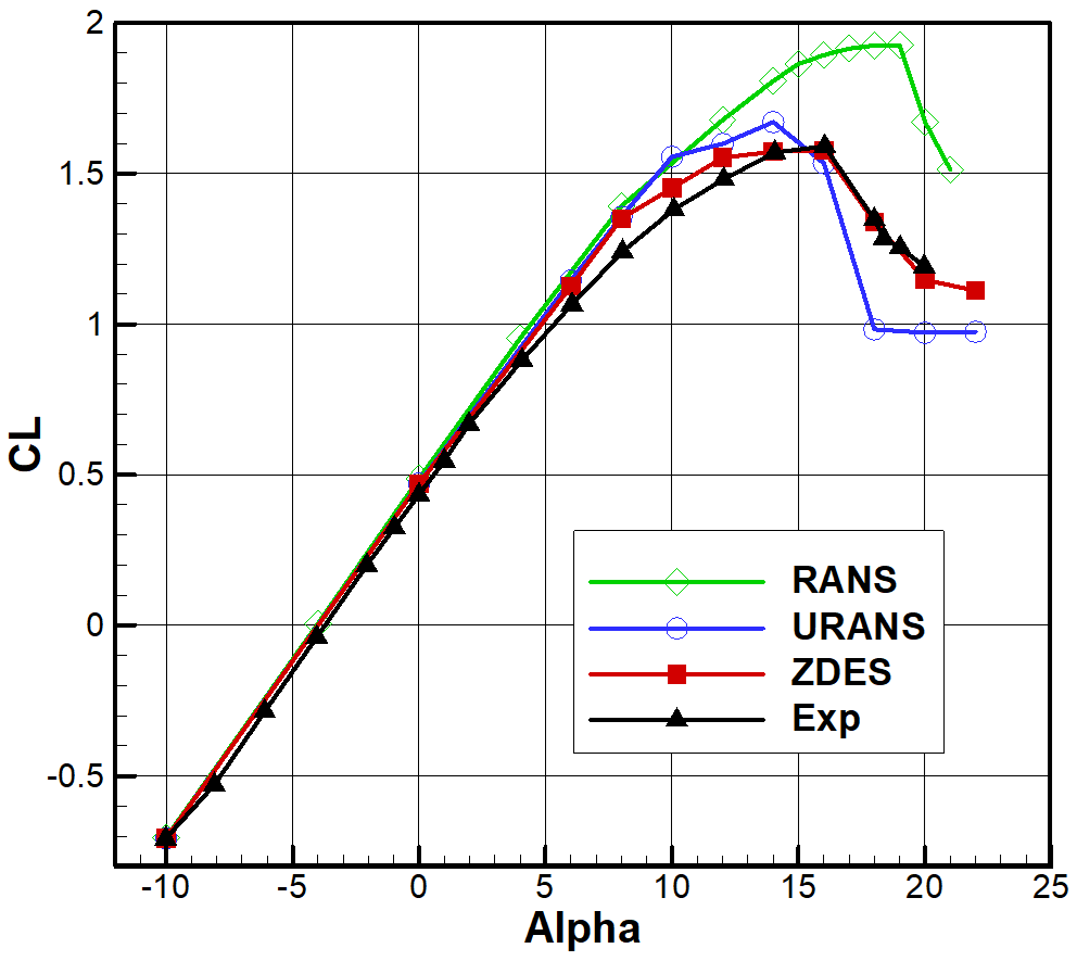
The stall AOA and maximum lift coefficient of the airfoil are overpredicted notably by RANS. The accuracy of the prediction of the stall AOA is improved with the application of URANS; however, the excessively sharp decreases in lift are both obtained using RANS and URANS under post-stall conditions.

(2)

The stall point predicted by ZDES is consistent with the experiment value; the gradual drop of lift is also obtained under the post-stall condition. The unsteady characteristics of lift during the stall process in the ZDES result are more pronounced than those in the URANS result.

(3)

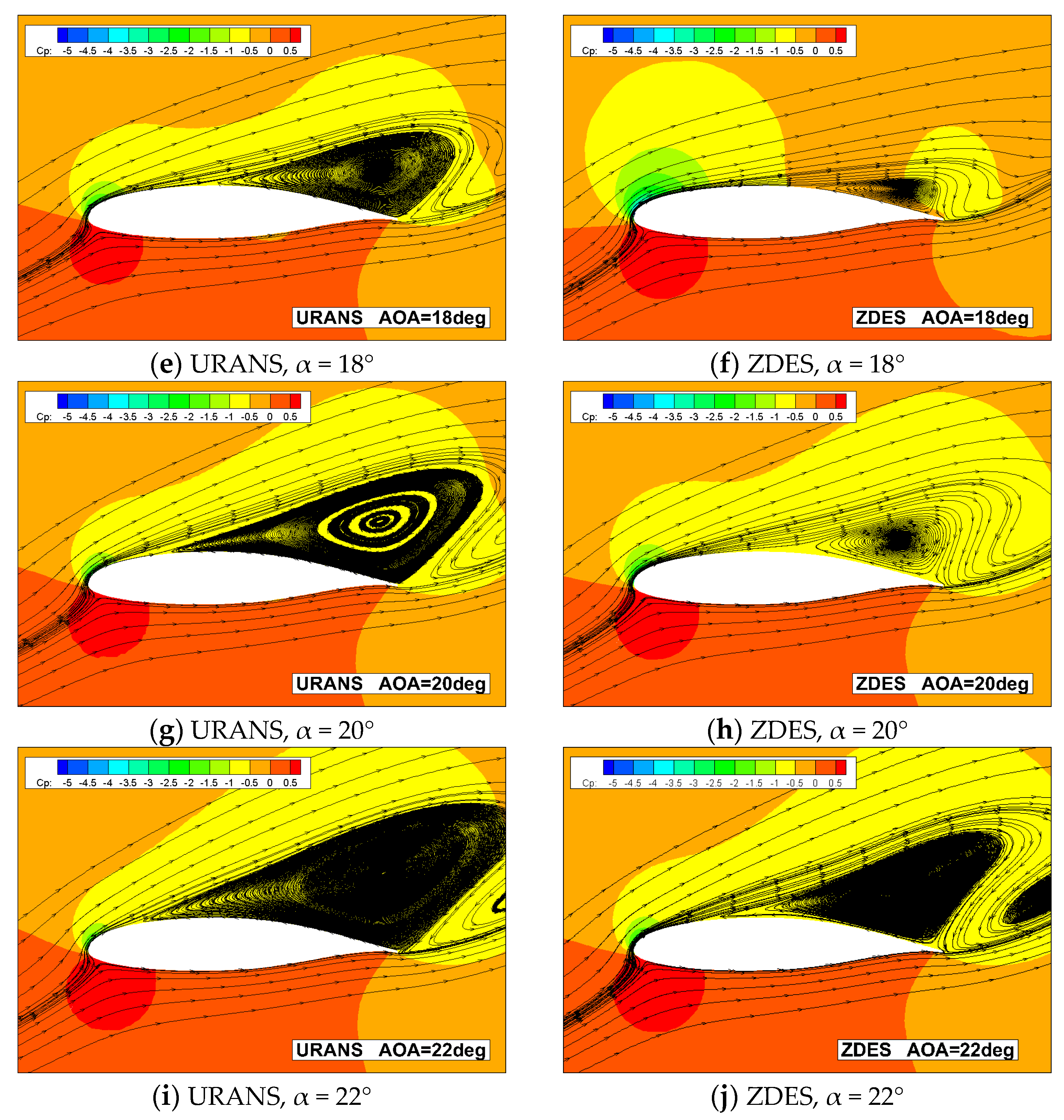
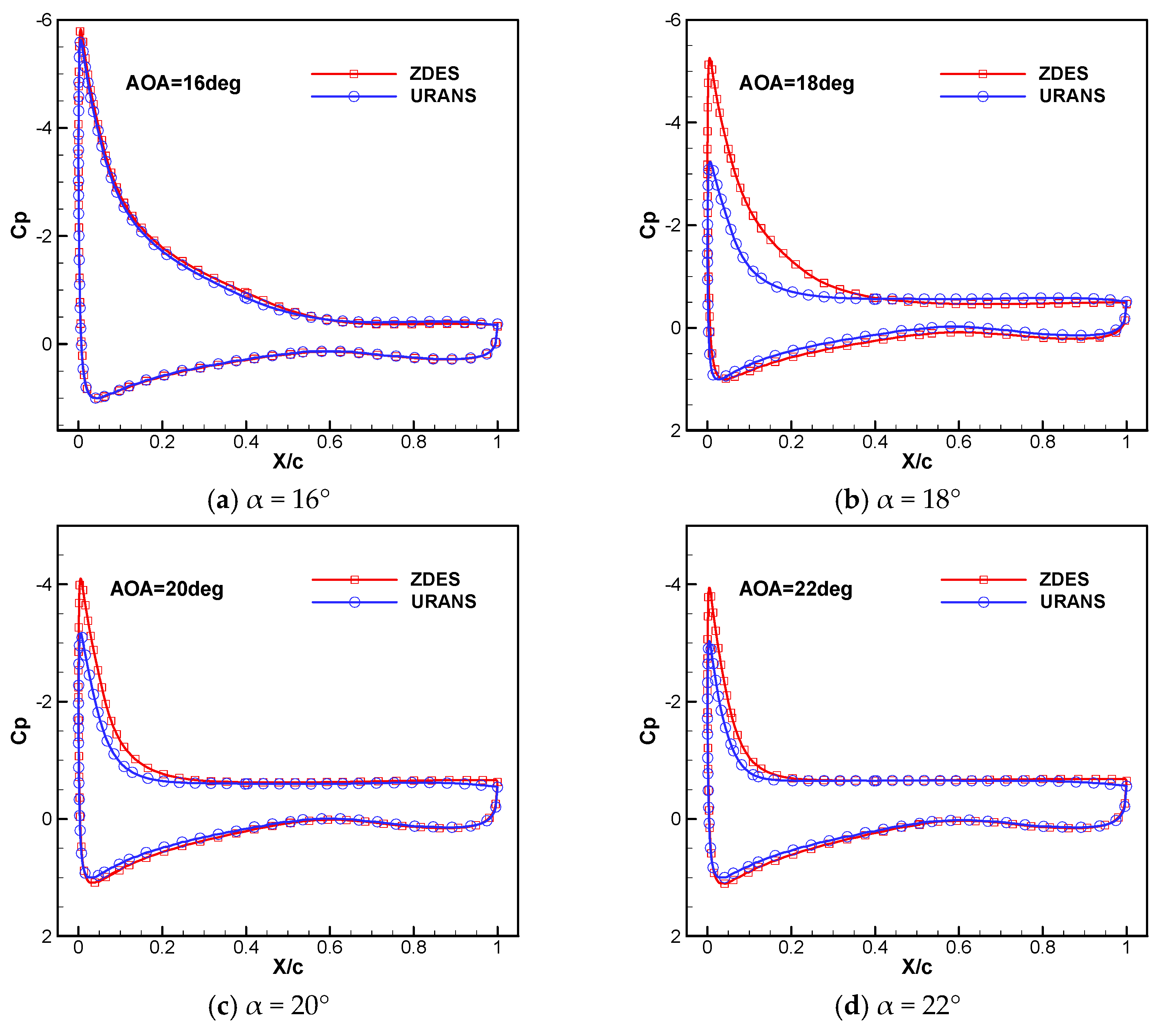
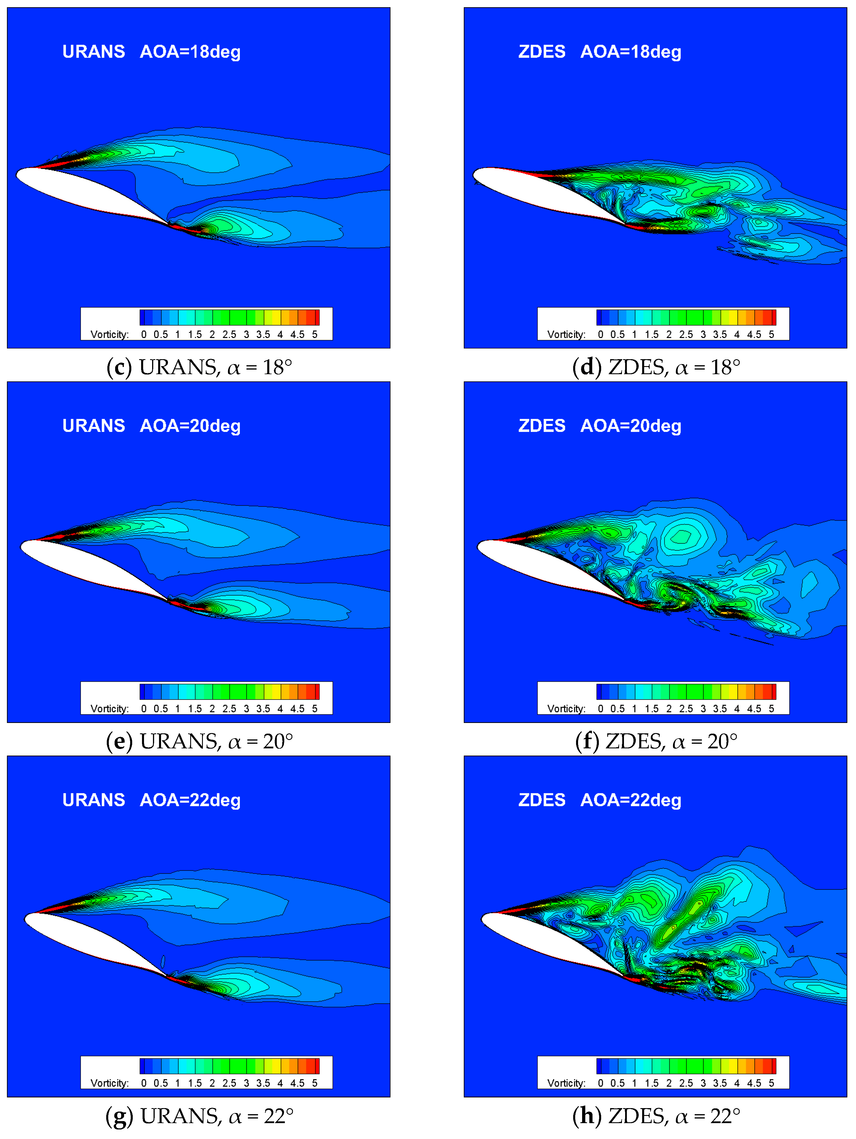
With the increase in the AOA, the expanding of the separation region at the trailing edge during the stall process are both predicted via URANS and ZDES, but a milder development of separation and decrease in leading edge peak suction are manifested in the ZDES result, which corresponds to a more reasonable stall prediction.

(4)

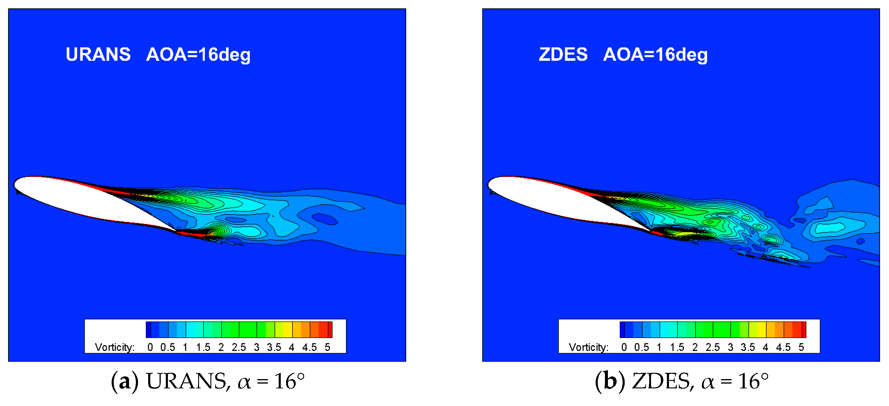
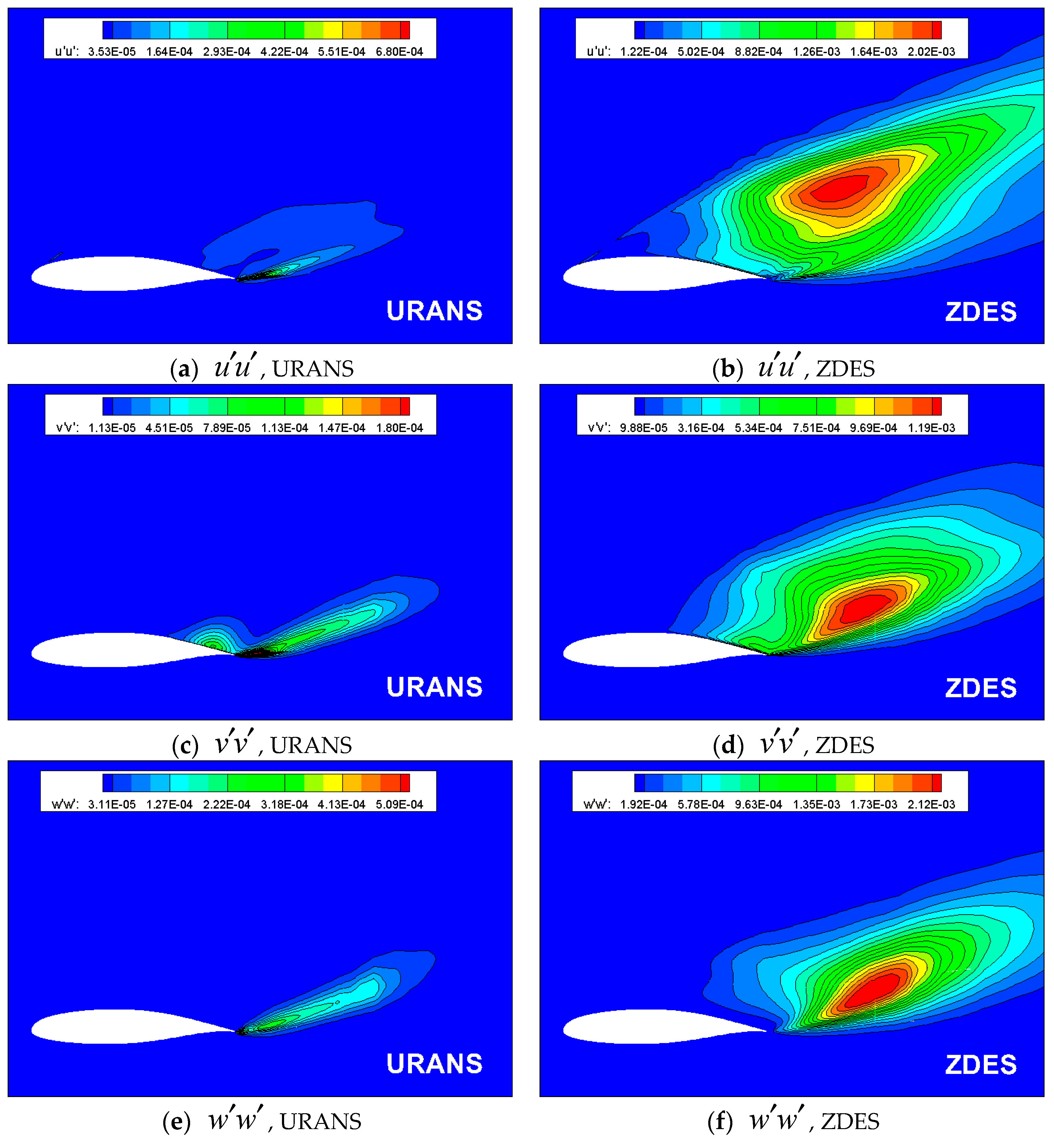
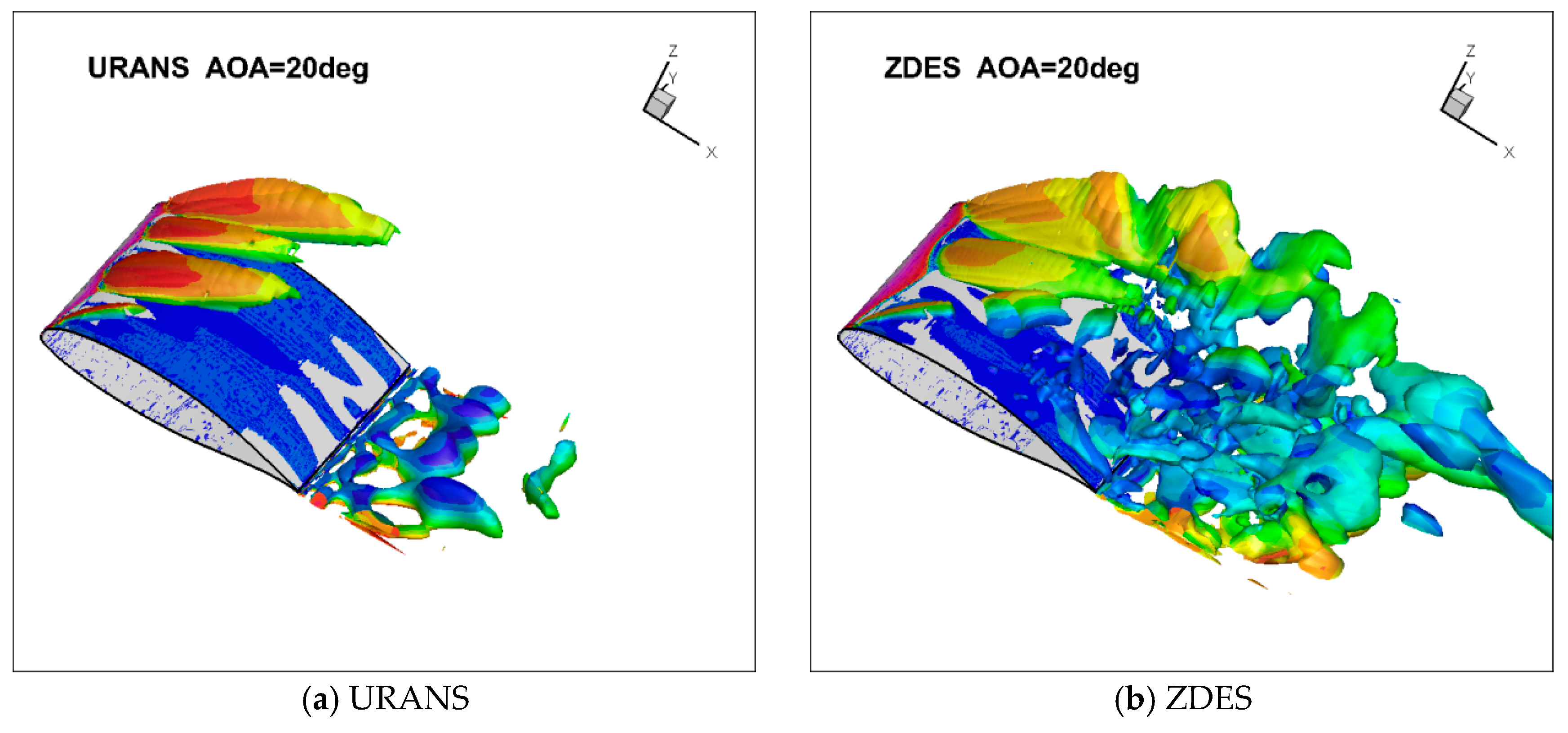
The alternate shedding and the interference of the leading edge and the trailing edge vortices are illustrated by ZDES near the stall point, while the core region of turbulent fluctuation is captured, which indicates the essential difference in the predicted stall result between URANS and ZDES.

(5)

From the result of ZDES, it is indicated that the core region of turbulent fluctuation is at the location far from the wall, where the interference of the leading edge and trailing edge vortices occurs. The phenomenon reveals the dominated flow behaviors under the post-stall condition of the trailing edge stall.

References

1. Mccullough, G.B.; Gault, D.E. Examples of Three Representative Types of Airfoil-Section Stall at Low Speed; NASA: Greenbelt, MD, USA, 1951; NACA-TN-2502. [Google Scholar]
2. Rhie, C.M.; Chow, W.L. Numerical study of the turbulent flow past an airfoil with trailing edge separation. AIAA J. 1983, 21, 1525–1532. [Google Scholar] [CrossRef]
3. Spalart, P.R. Detached-eddy simulation. Annu. Rev. Fluid Mech. 2009, 41, 181–202. [Google Scholar] [CrossRef]
4. Shur, M.; Spalart, P.R.; Strelets, M.; Travin, A. Detached-eddy simulation of an airfoil at high angle of attack. In Engineering Turbulence Modelling and Experiments; Elsevier Science Ltd.: London, UK, 1999; pp. 669–678. [Google Scholar]
5. Im, H.S.; Zha, G.C. Delayed detached eddy simulation of airfoil stall flows using high-order schemes. J. Fluids Eng. 2014, 136, 111104. [Google Scholar] [CrossRef]
6. Menter, F.R.; Kuntz, M. Adaptation of eddy-viscosity turbulence models to unsteady separated flow behind vehicles. In The Aerodynamics of Heavy Vehicles: Trucks, Buses, and Trains; Springer: Berlin/Heidelberg, 2004; pp. 339–352. [Google Scholar]
7. Yang, Y.; Zha, G.C. Simulation of airfoil stall flows using IDDES with high order schemes. In Proceedings of the 46th AIAA Fluid Dynamics Conference, Washington, DC, USA, 13–17 June 2016; p. 3185. [Google Scholar]
8. Shur, M.L.; Spalart, P.R.; Strelets, M.K.; Travin, A.K. A hybrid RANS-LES approach with delayed-DES and wall-modelled LES capabilities. Int. J. Heat Fluid Flow 2008, 29, 1638–1649. [Google Scholar] [CrossRef]
9. Wang, G.; Wang, S.; Li, H.; Fu, X.; Liu, W. Comparative assessment of SAS, IDDES and hybrid filtering RANS/LES models based on second-moment closure. Adv. Mech. Eng. 2021, 13, 16878140211028447. [Google Scholar] [CrossRef]
10. Gilling, L.; Sørensen, N.; Davidson, L. Detached eddy simulations of an airfoil in turbulent inflow. In Proceedings of the 47th AIAA Aerospace Sciences Meeting Including The New Horizons Forum and Aerospace Exposition, Orlando, FL, USA, 5–8 January 2009; p. 270. [Google Scholar]
11. Wang, L.; Li, L.; Fu, S. A comparative study of DES type methods for mild flow separation prediction on a NACA0015 airfoil. Int. J. Numer. Methods Heat Fluid Flow 2017, 27, 2528–2543. [Google Scholar] [CrossRef]
12. Guo, H.; Li, G.; Zou, Z. Numerical simulation of the flow around NACA0018 airfoil at high incidences by using RANS and DES methods. J. Mar. Sci. Eng. 2022, 10, 847. [Google Scholar] [CrossRef]
13. Li, D.; Men’shov, I.; Nakamura, Y. Detached-eddy simulation of three airfoils with different stall onset mechanisms. J. Aircr. 2006, 43, 1014–1021. [Google Scholar] [CrossRef]
14. Cokljat, D.; Liu, F. DES of turbulent flow over an airfoil at high incidence. In Proceedings of the 40th AIAA Aerospace Sciences Meeting & Exhibit, Reno, NV, USA, 14–17 January 2002; p. 590. [Google Scholar]
15. Durrani, N.; Qin, N. Behavior of detached-eddy simulations for mild airfoil trailing-edge separation. J. Aircr. 2011, 48, 193–202. [Google Scholar] [CrossRef]
16. Shur, M.L.; Spalart, P.R.; Strelets, M.K.; Travin, A.K. An enhanced version of DES with rapid transition from RANS to LES in separated flows. Flow Turbul. Combust. 2015, 95, 709–737. [Google Scholar] [CrossRef]
17. Yalçın, Ö.; Cengiz, K.; Özyörük, Y. High-order detached eddy simulation of unsteady flow around NREL S826 airfoil. J. Wind. Eng. Ind. Aerodyn. 2018, 179, 125–134. [Google Scholar] [CrossRef]
18. Deck, S. Recent improvements in the zonal detached eddy simulation (ZDES) formulation. Theor. Comput. Fluid Dyn. 2012, 26, 523–550. [Google Scholar] [CrossRef]
19. Le Pape, A.; Richez, F.; Deck, S. Zonal detached-eddy simulation of an airfoil in poststall condition. AIAA J. 2013, 51, 1919–1931. [Google Scholar] [CrossRef]
20. Richez, F.; Le Pape, A.; Costes, M. Zonal detached-eddy simulation of separated flow around a finite-span wing. AIAA J. 2015, 53, 3157–3166. [Google Scholar] [CrossRef]
21. Menter, F.R. Two-equation eddy-viscosity turbulence models for engineering applications. AIAA J. 1994, 32, 1598–1605. [Google Scholar] [CrossRef]
22. Chauvet, N.; Deck, S.; Jacquin, L. Zonal detached eddy simulation of a controlled propulsive jet. AIAA J. 2007, 45, 2458–2473. [Google Scholar] [CrossRef]
23. Zhang, X.; Zhang, H.; Li, J. Numerical Investigation of Stall Characteristics of Common Research Model Configuration Based on Zonal Detached Eddy Simulation Method. Aerospace 2023, 10, 817. [Google Scholar] [CrossRef]
24. Shi, W.; Zhang, H.; Li, Y. Enhancing the Resolution of Blade Tip Vortices in Hover with High-Order WENO Scheme and Hybrid RANS–LES Methods. Aerospace 2023, 10, 262. [Google Scholar] [CrossRef]
25. Zhang, H.; Li, J.; Jiang, Y.; Shi, W.; Jin, J. Analysis of the expanding process of turbulent separation bubble on an iced airfoil under stall conditions. Aerosp. Sci. Technol. 2021, 114, 106755. [Google Scholar] [CrossRef]
26. Shu, C.W. High order ENO and WENO schemes for computational fluid dynamics. In High-Order Methods for Computational Physics; Springer: Berlin/Heidelberg, Germany, 1999; pp. 439–582. [Google Scholar]
27. Whitcomb, R.T.; Clark, L.R. An Airfoil Shape for Efficient Flight at Supercritical Mach Numbers; NASA: Greenbelt, MD, USA, 1965; No. L-4517. [Google Scholar]
28. McGhee, R.J.; Bingham, G.J. Low-Speed Aerodynamic Characteristics of a 17-Percent-Thick Supercritical Airfoil Section, Including a Comparison between Wind-Tunnel and Flight Data; NASA: Greenbelt, MD, USA, 1972; No. L-8290. [Google Scholar]
29. Palmer, W.E.; Elliott, D.W.; White, J.E. Flight and Wind Tunnel Evaluation of a 17% Thick Supercritical Airfoil on a T-2C Airplane. In Vol. II-Flight Measured Wing Wake Profiles and Surface Pressures; North American Rockwell: Barberton, OH, USA, 1971; NR71H-150. [Google Scholar]
30. Xu, H.Y.; Qiao, C.L.; Yang, H.Q.; Ye, Z.Y. Delayed detached eddy simulation of the wind turbine airfoil S809 for angles of attack up to 90 degrees. Energy 2017, 118, 1090–1109. [Google Scholar] [CrossRef]
Figure 1. The definition of Δ ω of a grid cell.
Aerospace 11 00731 g001
Figure 2. The topology and section of the computational grid of LS-0417.
Aerospace 11 00731 g002
Figure 3. The definition of calculation region of ZDES.
Aerospace 11 00731 g003
Figure 4. The convergence history of the lift coefficient with different methods.
Aerospace 11 00731 g004
Figure 5. The convergence history of lift coefficient with different time steps.
Aerospace 11 00731 g005
Figure 6. Comparison of lift prediction results with different methods.
Aerospace 11 00731 g006
Figure 7. The convergence history of lift coefficient obtained with URANS and ZDES at different AOAs.
Aerospace 11 00731 g007aAerospace 11 00731 g007b
Figure 8. Comparison of time-averaged streamlines between URANS and ZDES.
Aerospace 11 00731 g008aAerospace 11 00731 g008b
Figure 9. Comparison of time-averaged pressure distribution between URANS and ZDES.
Aerospace 11 00731 g009
Figure 10. Comparison of instantaneous vorticity between URANS and ZDES.
Aerospace 11 00731 g010aAerospace 11 00731 g010b
Figure 11. Comparison of time-averaged turbulent fluctuation between URANS and ZDES, α = 20°.
Aerospace 11 00731 g011
Figure 12. Comparison of iso-surface of Q-criterion between URANS and ZDES.
Aerospace 11 00731 g012