
Two-Stage Hyperelliptic Kalman Filter-Based Hybrid Fault Observer for Aeroengine Actuator under Multi-Source Uncertainty

Abstract
1. Introduction
2. Mathematical Description of the Problem
3. Optimal Filtering under Multi-Source Uncertainty
3.1. PCE-Based UQ of Discrete Stochastic Model
3.1.1. Preliminaries of PCE
3.1.2. Statistical Property of Discrete Stochastic Model
3.2. Hyperelliptic Kalman Filter
4. Conservativeness-Reduced Fault Estimation under Multi-Source Uncertainty
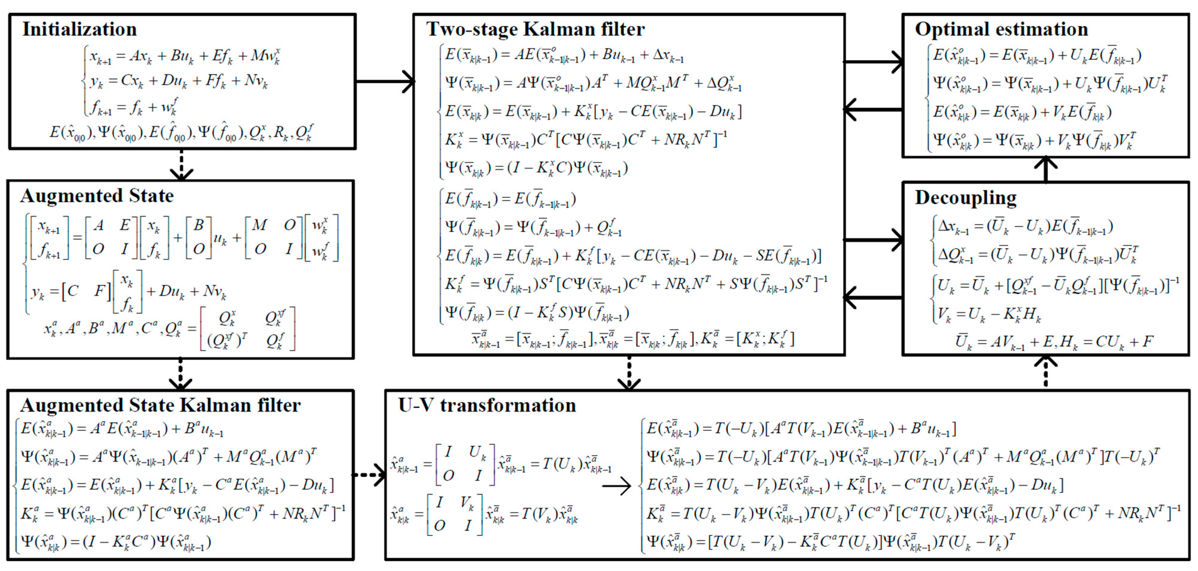
4.1. TSKF-Based Fault Estimation
4.2. TSHeKF-Based Optimal Estimation
- Augmented State estimator
- U-V transformations
- Decoupling
- Optimal estimation under multi-source uncertainty
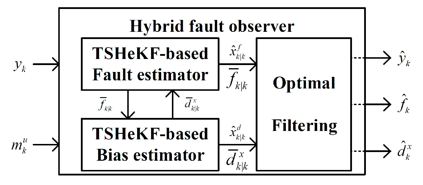
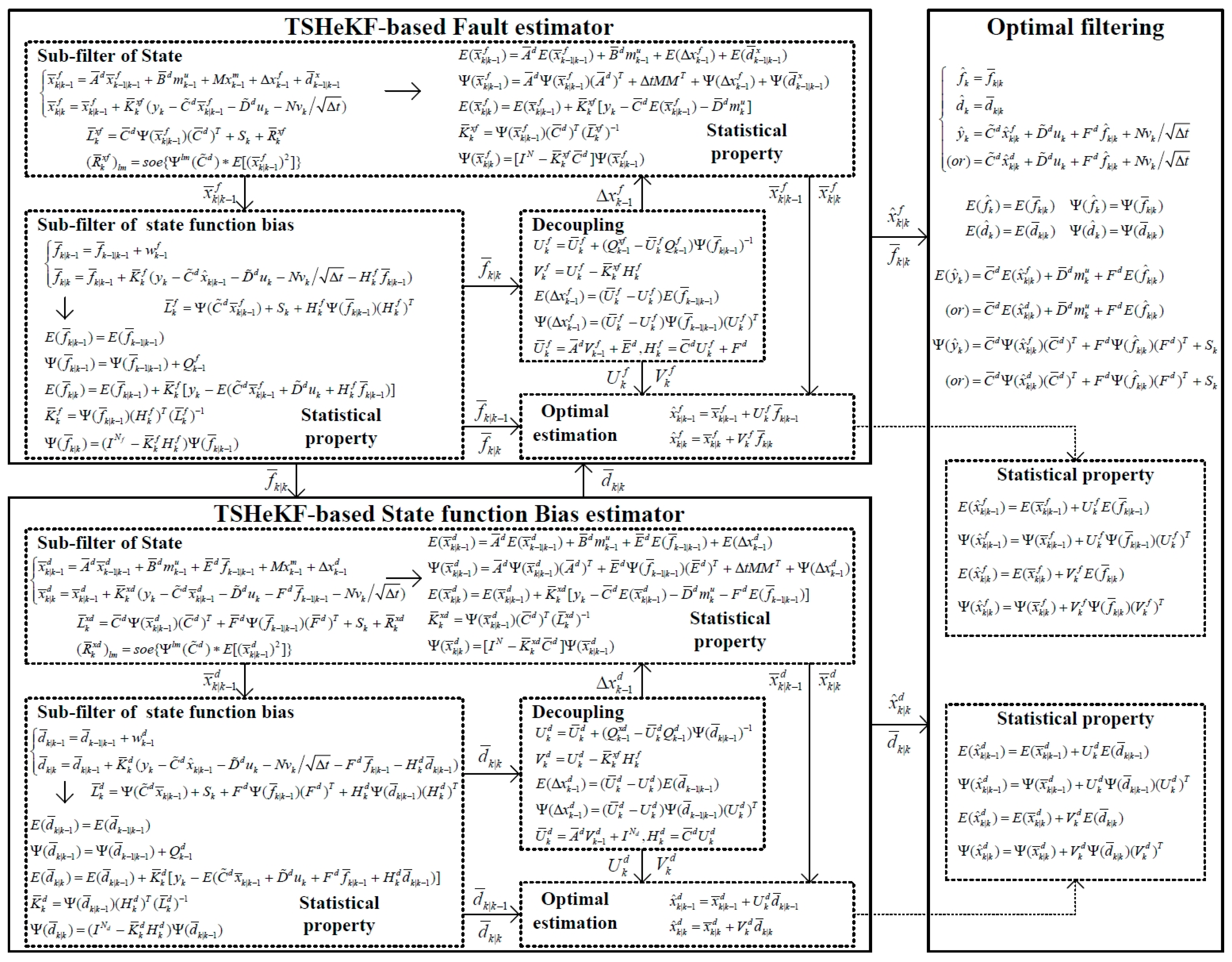
4.3. Conservativeness-Reduced Fault Estimation Based on HFO
5. Simulation
5.1. Linear Model under Multi-Source Uncertainty
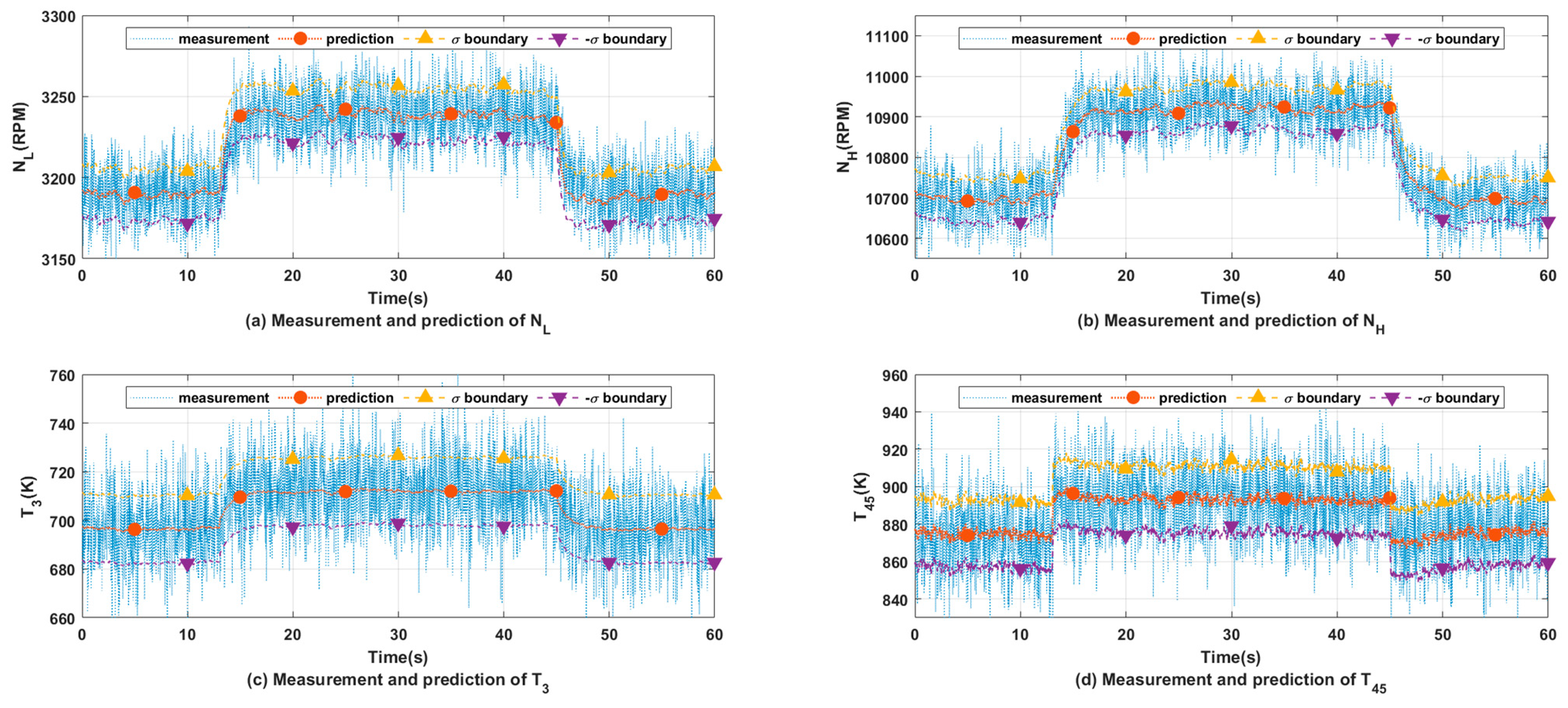
5.2. Optimal Filtering under Multi-Source Uncertainty
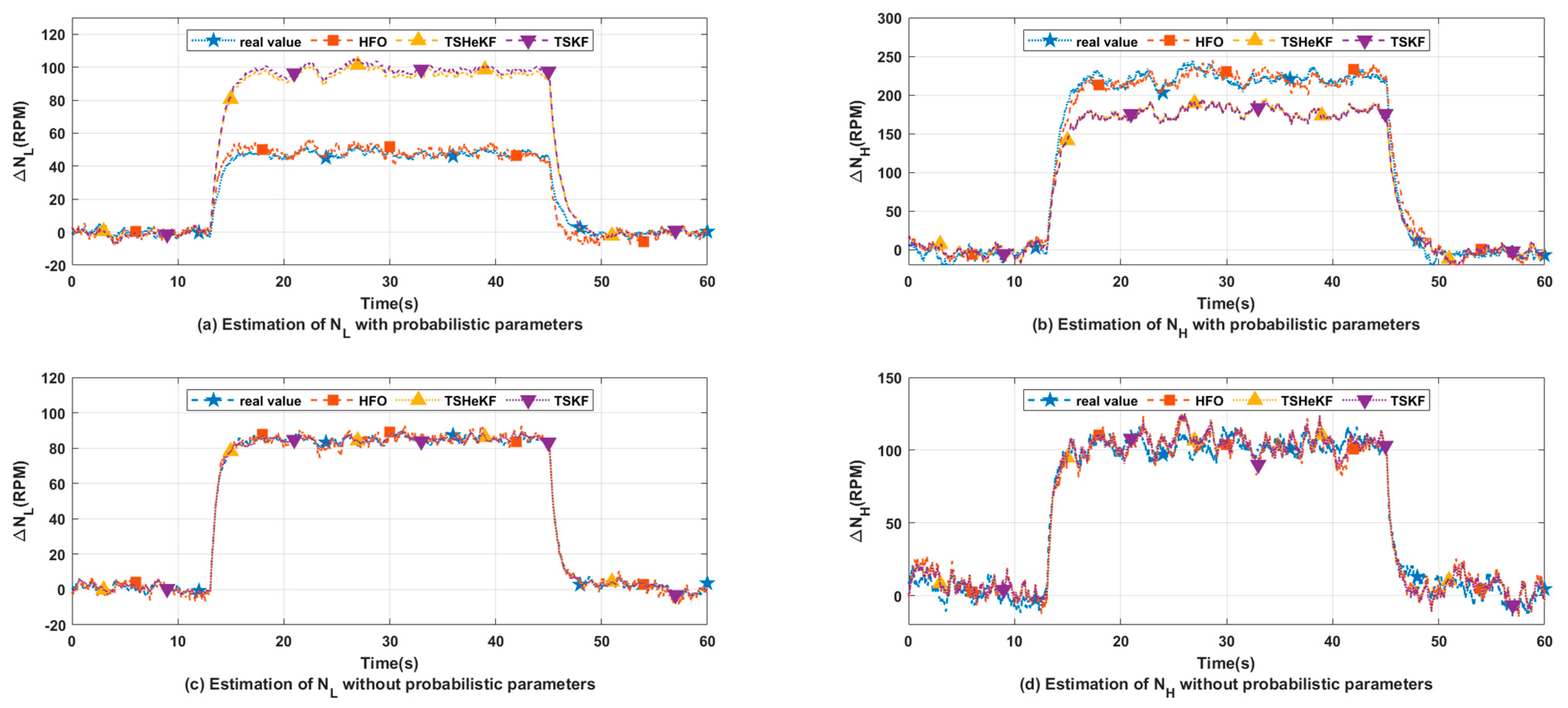
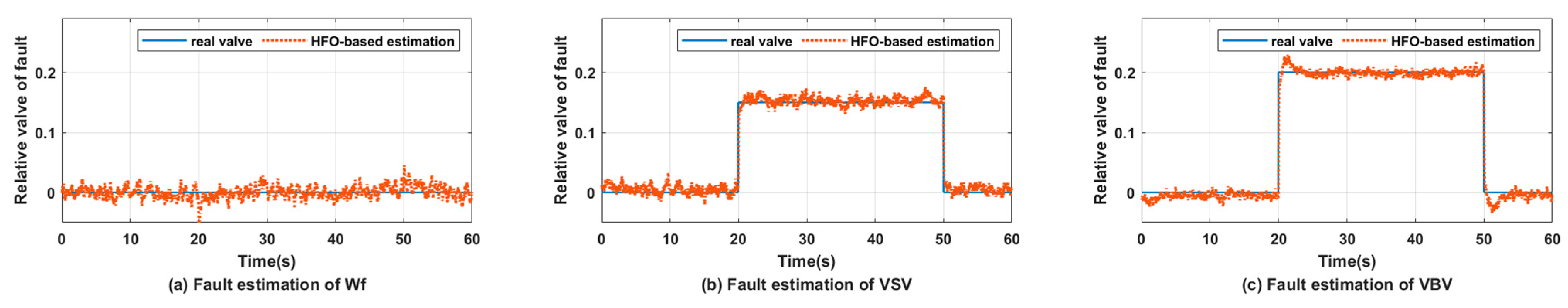
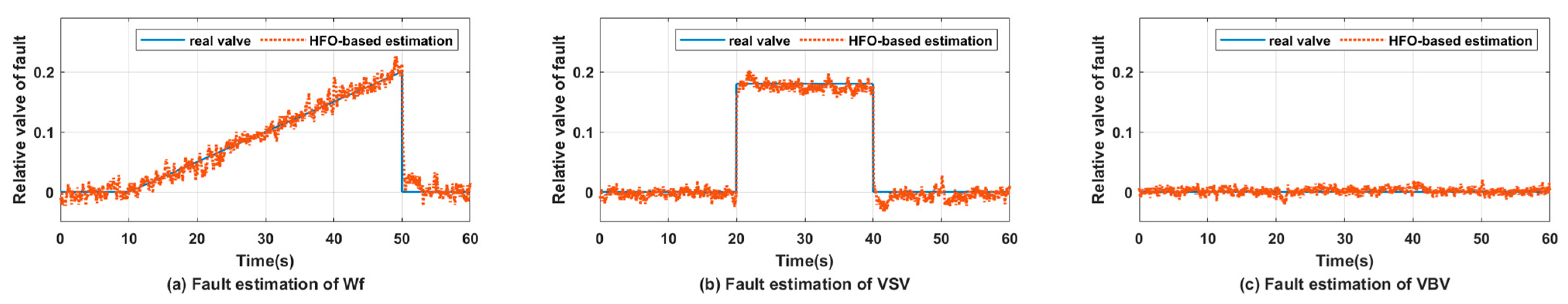
5.3. Actuator Optimal Fault Estimation
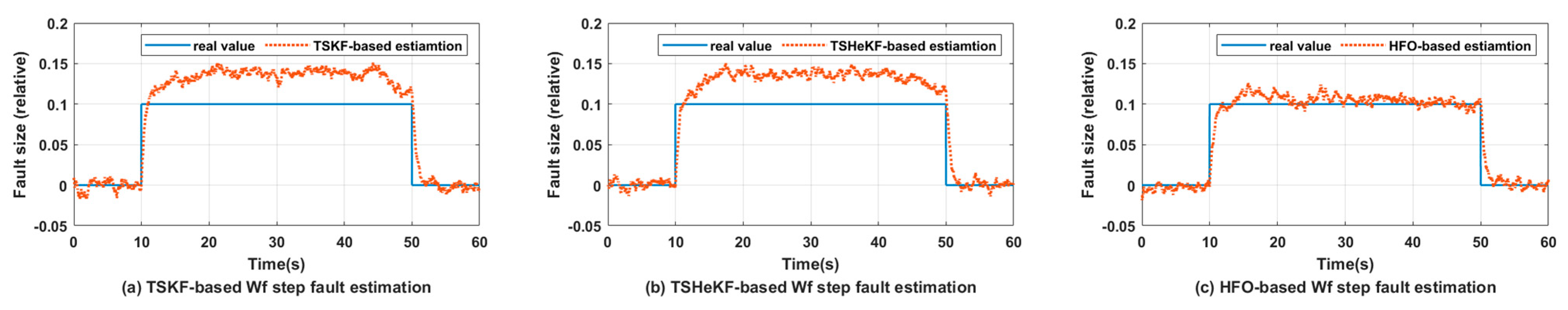
- : step fault of start from , with step fault of start from ; both faults last for .
- : step fault of and step fault of ; both last from to .
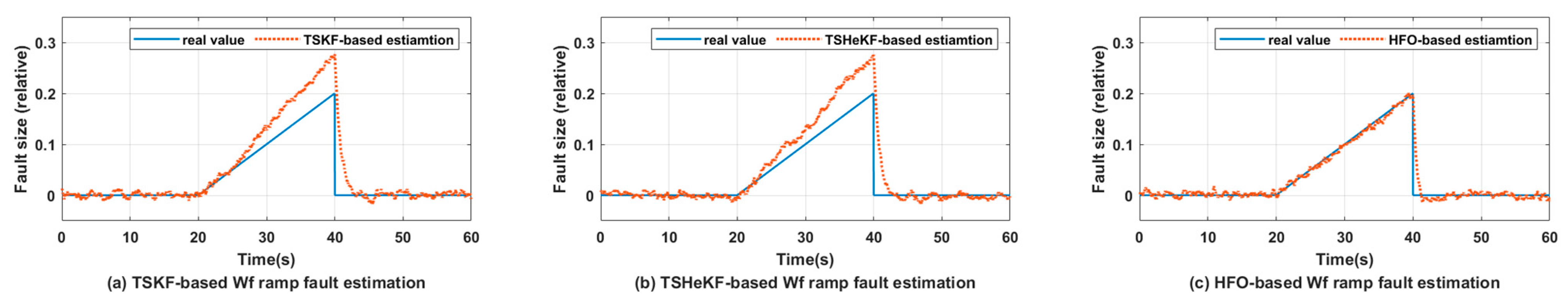
- : a ramp fault of with slope of from to , and a step fault of start at and last for .
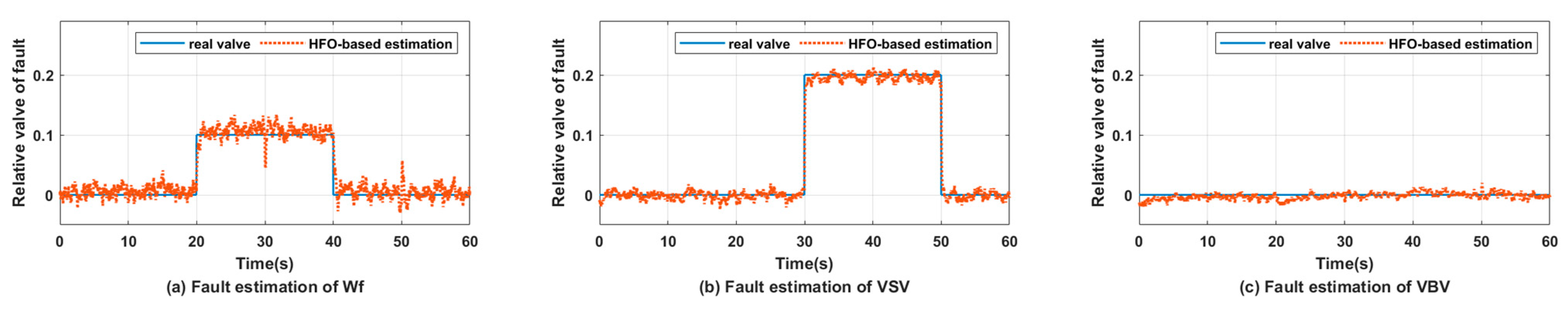
- : ramp faults of and , with slope of from to for and as slope starts from and stays at for .
- : ramp faults of and within to with slopes of and , respectively.
6. Conclusions
Author Contributions
Funding
Data Availability Statement
Conflicts of Interest
Abbreviation
| ASKF | Augmented State Kalman Filter |
| HFO | Hybrid Fault Observer |
| HeKF | Hyperelliptic Kalman Filter |
| LKF | Linear Kalman filter |
| MC | Monte Carlo |
| PCE | Polynomial Chaos Expansion |
| TSKF | Two-stage Kalman Filter |
| TSHeKF | Two-stage Hyperelliptic Kalman Filter |
| UQ | Uncertainty Quantification |
| ZKF | Zonotope Kalman Filter |
References
- Lv, C.; Chang, J.; Bao, W.; Yu, D. Recent research progress on airbreathing aero-engine control algorithm. Propuls. Power Res. 2022, 11, 1–57. [Google Scholar] [CrossRef]
- Rath, N.; Mishra, R.K.; Kushari, A. Aero engine health monitoring, diagnostics and prognostics for condition-based mainte-nance: An overview. Int. J. Turbo Jet Eng. 2024, 40, s279–s292. [Google Scholar] [CrossRef]
- Gou, L.; Sun, R.; Han, X. FDIA System for Sensors of the Aero-Engine Control System Based on the Immune Fusion Kalman Filter. Math. Probl. Eng. 2021, 2021, 6662425. [Google Scholar] [CrossRef]
- Roy, C.J.; Oberkampf, W.L. A comprehensive framework for verification, validation, and uncertainty quantification in sci-entific computing. Comput. Methods Appl. Mech. Eng. 2011, 200, 2131–2144. [Google Scholar] [CrossRef]
- Oberkampf, W.L.; Helton, J.C.; Joslyn, C.A.; Wojtkiewicz, S.F.; Ferson, S. Challenge problems: Uncertainty in system response given uncertain parameters. Reliab. Eng. Syst. Saf. 2004, 85, 11–19. [Google Scholar] [CrossRef]
- Sun, R.Q.; Han, X.B.; Chen, Y.X.; Gou, L.F. Hyperelliptic Kalman filter-based aeroengine sensor fault FDIA system under multi-source uncertainty. Aerosp. Sci. Technol. 2023, 132, 108058. [Google Scholar] [CrossRef]
- Liu, Z.; Wang, Z.; Wang, Y.; Ji, Z. Sensor fault estimation based on the constrained zonotopic Kalman filter. Int. J. Robust Nonlinear Control 2021, 31, 5984–6006. [Google Scholar] [CrossRef]
- Gou, L.; Shen, Y.; Zheng, H.; Zeng, X. Multi-Fault Diagnosis of an Aero-Engine Control System Using Joint Sliding Mode Observers. IEEE Access 2020, 8, 10186–10197. [Google Scholar] [CrossRef]
- Hamayun, M.T.; Edwards, C.; Alwi, H. Design and Analysis of an Integral Sliding Mode Fault-Tolerant Control Scheme. IEEE Trans. Autom. Control 2012, 57, 1783–1789. [Google Scholar] [CrossRef]
- Pourbabaee, B.; Meskin, N.; Khorasani, K. Sensor Fault Detection, Isolation, and Identification Using Multi-ple-Model-Based Hybrid Kalman Filter for Gas Turbine Engines. IEEE Trans. Control Syst. Technol. 2016, 24, 1184–1200. [Google Scholar] [CrossRef]
- Simon, D. A comparison of filtering approaches for aircraft engine health estimation. Aerosp. Sci. Technol. 2008, 12, 276–284. [Google Scholar] [CrossRef]
- Jin, P.; Lu, F.; Huang, J.; Kong, X.; Fan, M. Life cycle gas path performance monitoring with control loop parameters uncertainty for aeroengine. Aerosp. Sci. Technol. 2021, 115, 106775. [Google Scholar] [CrossRef]
- Lu, F.; Jiang, C.; Huang, J.; Qiu, X. A multi-rate sensor fusion approach using information filters for estimating aero-engine performance degradation. Chin. J. Aeronaut. 2019, 32, 1603–1617. [Google Scholar] [CrossRef]
- Hsieh, C.S.; Chen, F.C. Optimal solution of the two-stage Kalman estimator. IEEE Trans. Autom. Control 1999, 44, 194–199. [Google Scholar] [CrossRef]
- Hajiyev, C.; Cilden-Guler, D.; Hacizade, U. Two-Stage Kalman Filter for Fault Tolerant Estimation of Wind Speed and UAV Flight Parameters. Meas. Sci. Rev. 2020, 20, 35–42. [Google Scholar] [CrossRef]
- Chen, X.; Sun, R.; Wang, F.; Song, D.; Jiang, W. Two-stage unscented Kalman filter algorithm for fault estimation in space-craft attitude control system. IET Control Theory A 2018, 12, 1781–1791. [Google Scholar] [CrossRef]
- Patton, R.J.; Chen, J. On eigenstructure assignment for robust fault diagnosis. Int. J. Robust Nonlinear Control 2000, 10, 1193–1208. [Google Scholar] [CrossRef]
- Zhou, D.; Ma, S.; Chen, Y.; Wei, T.; Zhang, H.; Wei, F. A gas path fault diagnostic model for gas turbine based on deep belief network with prior information. In Proceedings of the 2018 IEEE International Conference on Prognostics and Health Management (ICPHM), Seattle, WA, USA, 11–13 June 2018; pp. 1–6. [Google Scholar]
- Lu, F.; Huang, J.; Lv, Y. Gas Path Health Monitoring for a Turbofan Engine Based on a Nonlinear Filtering Approach. Energies 2013, 6, 492–513. [Google Scholar] [CrossRef]
- Combastel, C. Zonotopes and Kalman observers: Gain optimality under distinct uncertainty paradigms and robust convergence. Automatica 2015, 55, 265–273. [Google Scholar] [CrossRef]
- Zhang, W.; Wang, Z.; Guo, S.; Shen, Y. Interval estimation of sensor fault based on zonotopic Kalman filter. Int. J. Control 2021, 94, 1641–1650. [Google Scholar] [CrossRef]
- Xiu, D. Numerical Methods for Stochastic Computations: A Spectral Method Approach; Princeton University Press: Princeton, NJ, USA, 2010; p. 125. [Google Scholar]
- Dutta, P.; Bhattacharya, R. Nonlinear estimation with polynomial chaos and higher order moment updates. In Proceedings of the 2010 American Control Conference, Baltimore, MD, USA, 30 June–2 July 2010; pp. 3142–3147. [Google Scholar]
- Dutta, P.; Bhattacharya, R. Nonlinear Estimation of Hypersonic Flight Using Polynomial Chaos. In Proceedings of the AIAA Guidance, Navigation, and Control Conference, Toronto, ON, Canada, 2–5 August 2010. [Google Scholar]
- Sun, R.-Q.; Gou, L.-F.; Liu, Z.-Y.; Han, X.-B. Three-stage hyperelliptic Kalman filter for health and performance monitoring of aeroengine under multi-source uncertainty. Int. J. Engine Res. 2023, 25, 557–572. [Google Scholar]
- Ding, S.X. Model-Based Fault Diagnosis Techniques: Design Schemes, Algorithms and Tools; Springer: New York, NY, USA, 2013. [Google Scholar]
- Øksendal, B. Stochastic Differential Equations: An Introduction with Applications; Spring: New York, NY, USA, 2003. [Google Scholar]
- Xia, B.; Wu, H.; Qiu, Y.; Lou, B.; Song, Y. A Galerkin Method-Based Polynomial Approximation for Parametric Problems in Power System Transient Analysis. IEEE Trans. Power Syst. 2019, 34, 1620–1629. [Google Scholar] [CrossRef]
- Manfredi, P.; De Zutter, D.; Ginste, D.V. On the relationship between the stochastic Galerkin method and the pseudo-spectral collocation method for linear differential algebraic equations. J. Eng. Math. 2018, 108, 73–90. [Google Scholar] [CrossRef]
- Oladyshkin, S.; Nowak, W. Data-driven uncertainty quantification using the arbitrary polynomial chaos expansion. Reliab. Eng. Syst. Saf. 2012, 106, 179–190. [Google Scholar] [CrossRef]
- Shin, Y.; Xiu, D. Nonadaptive quasi-optimal points selection for least squares linear regression. SIAM. J. Sci. Comput. 2016, 38, A385–A411. [Google Scholar] [CrossRef]
- Constantine, P.G.; Gleich, D.F.; Iaccarino, G. Spectral methods for parameterized matrix equations. SIAM J. Matrix Anal. Appl. 2010, 31, 2681–2699. [Google Scholar] [CrossRef]
- Oladyshkin, S.; Nowak, W. Incomplete statistical information limits the utility of high-order polynomial chaos expansions. Reliab. Eng. Syst. Saf. 2018, 169, 137–148. [Google Scholar] [CrossRef]
- Hsieh, C.S. Robust two-stage Kalman filters for systems with unknown inputs. IEEE Trans. Autom. Control 2000, 45, 2374–2378. [Google Scholar] [CrossRef]
- Montomoli, F.; Carnevale, M.; D’Ammaro, A.; Massini, M.; Salvadori, S. Uncertainty Quantification in Computational Fluid Dynamics and Aircraft Engines; Springer: Cham, Switzerland, 2019. [Google Scholar]
- Gou, L.; Zeng, X.; Wang, Z.; Han, G.; Lin, C.; Cheng, X. A Linearization Model of Turbofan Engine for Intelligent Analysis Towards Industrial Internet of Things. IEEE Access 2019, 7, 145313–145323. [Google Scholar] [CrossRef]


| Control Variable | Relative Error (%) | Nominal Value |
|---|---|---|
| 2.0 | 0.75 | |
| 5.0 | −13.62° | |
| 5.0 | 0.52° |
| Output Variable | Relative Error (%) | Nominal Value |
|---|---|---|
| 0.5 | 3190 | |
| 0.5 | ||
| 0.5 | ||
| 0.5 | ||
| 2.0 | ||
| 2.0 | ||
| 2.0 |
| Drive Matrix | Value |
|---|---|
| Control Matrix | Expectation | Standard Deviation |
|---|---|---|
| () | ||
| () | ||
| Method | Index | Relative Error of Output Prediction (%) | ||||||
|---|---|---|---|---|---|---|---|---|
| TSKF | Min | 0.382 | 0.385 | 0.389 | 0.389 | 1.513 | 1.530 | 1.519 |
| Mean | 0.507 | 0.408 | 0.412 | 0.412 | 1.585 | 1.619 | 1.627 | |
| Max | 2.679 | 0.945 | 0.562 | 0.580 | 1.656 | 3.150 | 3.012 | |
| TSHeKF | Min | 0.376 | 0.377 | 0.381 | 0.376 | 1.512 | 1.531 | 1.520 |
| Mean | 0.493 | 0.399 | 0.404 | 0.398 | 1.584 | 1.609 | 1.617 | |
| Max | 2.511 | 0.892 | 0.527 | 0.511 | 1.655 | 3.084 | 2.989 | |
| HFO | Min | 0.367 | 0.375 | 0.359 | 0.370 | 1.512 | 1.530 | 1.516 |
| Mean | 0.386 | 0.395 | 0.383 | 0.391 | 1.584 | 1.591 | 1.598 | |
| Max | 0.404 | 0.419 | 0.407 | 0.412 | 1.656 | 1.668 | 1.689 | |
| Method | Relative Error of Fault Estimation | Input Noise Intensity | |||||
|---|---|---|---|---|---|---|---|
| 2% | 4% | 6% | 8% | 10% | |||
| TSKF | Mean | Min | 0.056 | 0.066 | 0.074 | 0.081 | 0.089 |
| Mean | 0.183 | 0.224 | 0.278 | 0.329 | 0.373 | ||
| Max | 1.518 | 1.927 | 2.485 | 3.025 | 3.471 | ||
| Standard deviation | 0.160 | 0.196 | 0.245 | 0.290 | 0.326 | ||
| TSHeKF | Mean | Min | 0.055 | 0.070 | 0.081 | 0.094 | 0.108 |
| Mean | 0.178 | 0.191 | 0.211 | 0.231 | 0.248 | ||
| Max | 1.624 | 1.703 | 1.860 | 2.010 | 2.127 | ||
| Standard deviation | 0.157 | 0.159 | 0.168 | 0.177 | 0.184 | ||
| HFO | Mean | Min | 0.054 | 0.060 | 0.068 | 0.077 | 0.092 |
| Mean | 0.086 | 0.102 | 0.121 | 0.142 | 0.166 | ||
| Max | 0.218 | 0.2288 | 0.2498 | 0.287 | 0.350 | ||
| Standard deviation | 0.023 | 0.022 | 0.023 | 0.027 | 0.032 | ||
Disclaimer/Publisher’s Note: The statements, opinions and data contained in all publications are solely those of the individual author(s) and contributor(s) and not of MDPI and/or the editor(s). MDPI and/or the editor(s) disclaim responsibility for any injury to people or property resulting from any ideas, methods, instructions or products referred to in the content. |
© 2024 by the authors. Licensee MDPI, Basel, Switzerland. This article is an open access article distributed under the terms and conditions of the Creative Commons Attribution (CC BY) license (https://creativecommons.org/licenses/by/4.0/).
Share and Cite
Wang, Y.; Sun, R.-Q.; Gou, L.-F. Two-Stage Hyperelliptic Kalman Filter-Based Hybrid Fault Observer for Aeroengine Actuator under Multi-Source Uncertainty. Aerospace 2024, 11, 736. https://doi.org/10.3390/aerospace11090736
Wang Y, Sun R-Q, Gou L-F. Two-Stage Hyperelliptic Kalman Filter-Based Hybrid Fault Observer for Aeroengine Actuator under Multi-Source Uncertainty. Aerospace. 2024; 11(9):736. https://doi.org/10.3390/aerospace11090736
Chicago/Turabian StyleWang, Yang, Rui-Qian Sun, and Lin-Feng Gou. 2024. "Two-Stage Hyperelliptic Kalman Filter-Based Hybrid Fault Observer for Aeroengine Actuator under Multi-Source Uncertainty" Aerospace 11, no. 9: 736. https://doi.org/10.3390/aerospace11090736
APA StyleWang, Y., Sun, R.-Q., & Gou, L.-F. (2024). Two-Stage Hyperelliptic Kalman Filter-Based Hybrid Fault Observer for Aeroengine Actuator under Multi-Source Uncertainty. Aerospace, 11(9), 736. https://doi.org/10.3390/aerospace11090736