An Open-Source Code for High-Speed Non-Equilibrium Gas–Solid Flows in OpenFOAM

Abstract

This paper details the development and verification tests of an open-source code named hy2LPTFoam intended for solving high-speed non-equilibrium gas-particle flows in OpenFOAM. The solver, based on hy2Foam for high-speed non-equilibrium gas flow, integrates multiple particle force models, heat transfer models, the diffusion-based smoothing method, and the MPPIC method. The verification tests incorporate interactions between shock waves and particle curtains with varying particle volume fractions, a JPL nozzle generating a two-phase gas–particle flow, and a Mars entry body with two particle inflow mass fractions. The tests yield good physical agreement with numerical and experimental data from the literature.

1. Introduction

Deeper exploration of space encounters an increasing number of non-equilibrium high-speed gas–particle two-phase flow scenarios in the extraterrestrial and space environments, such as the example of Mars atmospheric re-entry in the presence of sandstorms [1] shown in Figure 1 and the plume–regolith surface interaction during a soft landing maneuver shown in [2] Figure 2. Such gas–particle flows are significantly complex due to the presence of non-equilibrium effects, gas–particle momentum and energy coupling at both the micro- and macroscopic levels, and particle–particle interactions.

Since Park successfully extended the range of applicability of the Navier–Stokes–Fourier equations by developing the two-temperature model [3], many numerical tools for solving non-equilibrium high-speed gas flow have been widely developed, including DPLR (Data-Parallel Line Relaxation) [4], LAURA (Langley Aerothermodynamic Upwind Relaxation Algorithm) [5], URANUS (Upwind Relaxation Algorithm for Nonequilibrium Flows of the University of Stuttgart) [6], US3D [7], HRF (Hypersonic Reacting Flow) [8], hy2Foam [9], hyperReactingFoam [10], and Eilmer [11]. In particular, in-house codes such as the Sequential Iterative Non-equilibrium Algorithm (SINA) [12] and US3D [13,14] have been extended to incorporate Lagrangian particle tracking module in order to study Mars entry problems. Additionally, a density-based in-house solver, rhoCentralFoam [15] in OpenFOAM, has been modified and developed into a new solver named RYrhoCentralFoam [16] for solving multi-phase, multi-component, compressible, and reacting flows with low particle concentration. Zhang et al. [17] later broadened the particle volume fraction to a moderate level at which particle–particle collisions are significant. Ching et al. [18] developed a high-order two-way coupled Euler–Lagrange method based on discontinuous Galerkin schemes and benchmarked the code with high-speed dusty flow with small particle volume fraction; however, the non-equilibrium gas effect in hypersonic condition is not considered in this high-order code.

Open-source non-equilibrium high-speed gas–particle flow solvers are less common than the solvers for solving hypersonic flows. The existing codes are built either with limited accessibility to the public or on an uneven level and lack of integration of particle models. There is demand for an open-source code for use in conducting simulations for research and education.

As such, this work develops an open-source solver called hy2LPTFoam in OpenFOAM. The solver is based on hy2Foam [9], which is an open-source density-based Navier–Stokes–Fourier code for solving non-equilibrium hypersonic flows. The existing hy2Foam library is fully in charge of the gas flow, and a new class called LPT is responsible for the particle evolution. The hy2LPTFoam solver integrates multiple common particle force models, heat transfer models, the diffusion-based smoothing method, and the Multi-Phase Particle-Pn-Cell (MPPIC) method [19,20,21,22,23], which has been extensively used in gas–particle flows. The solver can cover a wide range of flow conditions.

The remainder of the paper is organized as follows: Section 2 describes the algorithm of the solver and outlines the governing equations of both gas and particles, followed by introduction of the interphase coupling method. The subsequent section focuses on results for three test cases, including shock–particle curtain interactions in shock tubes, gas–particle flow in a JPL nozzle, and hypersonic two-phase flow during Mars entry.

2. Methodology

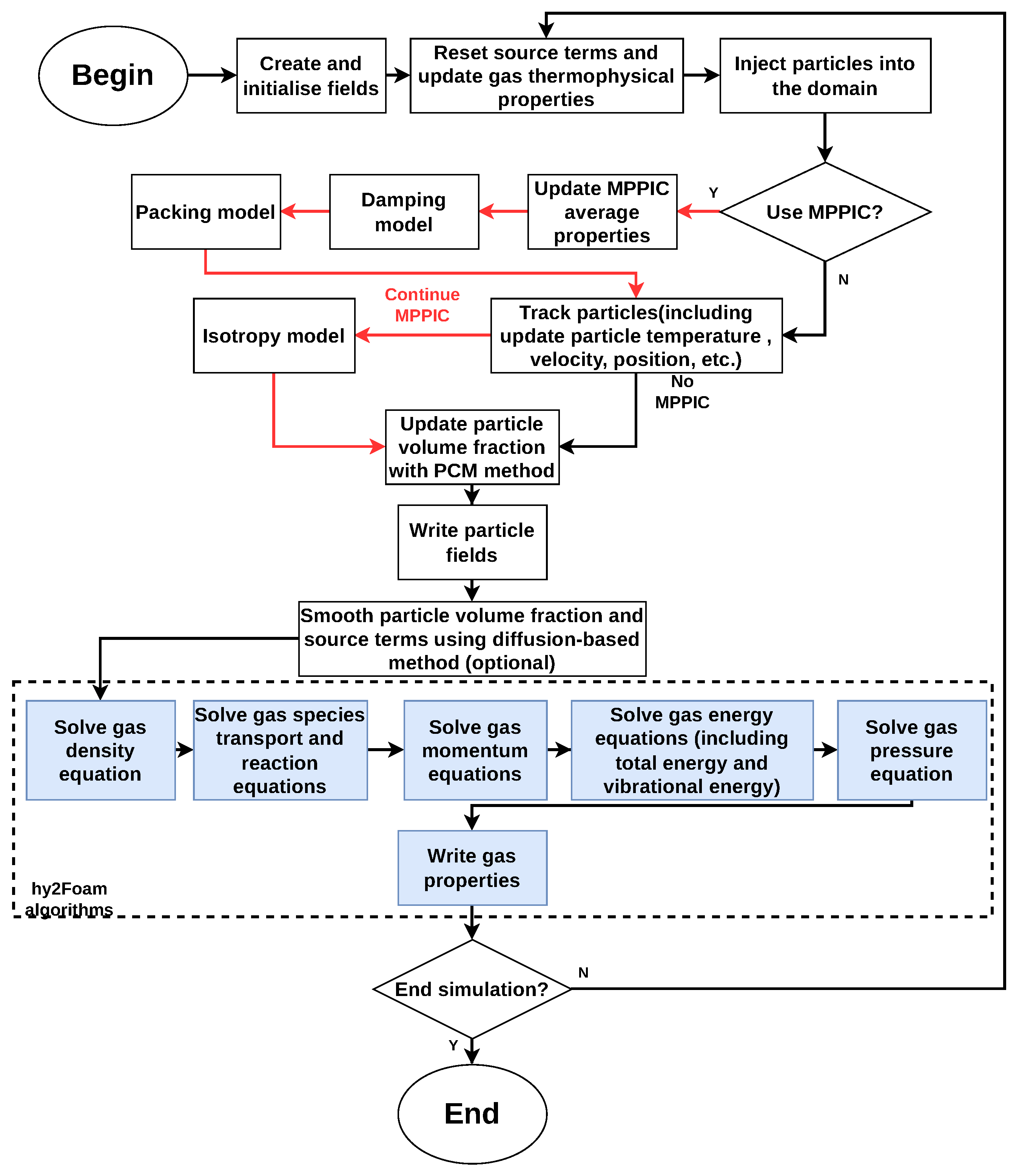
2.1. Algorithmic Overview

The basic algorithm of hy2LPTFoam is presented in Figure 3:

• Step 1: Calculation of the gas phase thermophysical properties necessary to calculate the particle drag force and reset the source terms of the particle phase.
• Step 2: Injection of particles from inlet boundaries.
• Step 3: Evolution of the disperse phase, including performing particle movements, updating temperatures, velocities and positions, and conducting Multi-Phase Particle-In-Cell (MPPIC) procedures (optional).
• Step 4: Sampling and calculation of discrete phase properties and returning the desired macroscopic fields, such as number density and surface heat flux.
• Step 5: Updating the particle volume fraction using the particle cell method.
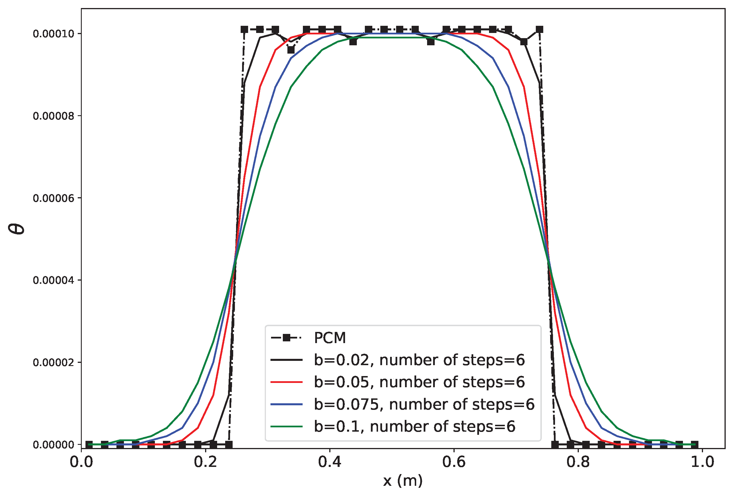
• Step 6: Smoothing the particle volume fraction and source terms using the diffusion-based method (optional).
• Step 7: Solving the continuity, momentum, and energy equations of the gas phase and entering the gas properties in the hy2Foam algorithm.
• Step 8: Return to Step 1 until the time reaches the final calculation time.

2.2. Governing Equations of Gas Phase

The hy2Foam [9] is an open-source density-based Navier–Stokes–Fourier code designed to solve hypersonic flow problems. These problems are characterized by high Mach numbers and chemical reactions. The model operates under a two-temperature assumption, where both translational and rotational temperatures equate to a trans-rotational temperature. Additionally, it assumes that the electron, electronic energy, and vibrational energy temperatures are equivalent to a single vibrational-electron-electronic temperature. This solver is particularly adept at simulating high-speed flows in the near-continuum regime, a task that is computationally demanding when using Direct Simulation of Monte Carlo (DSMC) solvers. The hy2Foam solver has been rigorously tested and validated under conditions with and without chemical reactions in hypersonic flow environments. The hy2Foam solver is derived from the rhoCentralFoam solver, thereby incorporating the central-upwind differencing schemes of Kurganov and Tadmor. It has been extensively applied in solving hypersonic vehicle problems [24], planetary entry scenarios [9], and supersonic flow physics within near-continuum flow regimes [25].

The non-equilibrium Navier–Stokes–Fourier equations for a mixture of $N_i$ gas species and $N_m$ molecules with the consideration of particle volume fraction effect are expressed as follows:

$${\displaystyle \frac{\partial \theta \rho }{\partial t}}+\nabla ·(\theta \rho \overrightarrow{v})=0$$

(1)

$${\displaystyle \frac{\partial \theta \rho Y_i}{\partial t}}+\nabla ·(\theta \rho Y_i\overrightarrow{v})=\nabla \theta J_i+{\dot{\omega }}_i$$

(2)

$${\displaystyle \frac{\partial \theta \rho \overrightarrow{v}}{\partial t}}+\nabla ·(\theta \rho \overrightarrow{v}\overrightarrow{v})=-\theta \nabla p+\nabla ·\left\{\theta \mathit{\tau }\right\}+Sv$$

(3)

$${\displaystyle \frac{\partial \theta {\rho }_i{e}_{ve,m}}{\partial t}}+\nabla ·(\theta {\rho }_i{e}_{ve,m}\overrightarrow{v})=q_{ve,m}+\nabla \theta e_{ve,m}{J}_m+{\dot{\omega }}_{v,m}$$

(4)

$${\displaystyle \frac{\partial \theta \rho e}{\partial t}}+\nabla ·(\theta \rho e\overrightarrow{v})=-\nabla ·(\theta p\overrightarrow{v})+\nabla ·\{\theta \mathit{\tau }·\overrightarrow{v}\}-q_{tr}-q_{ve}-\nabla (\theta \sum h_r{J}_r)+Se$$

(5)

where:

$$q_{tr}=-{\kappa }_{tr}\nabla T_{tr}$$

(6)

$$q_{ve}=\sum -{\kappa }_{ve,i}\nabla T_{ve,i}$$

(7)

in which $\rho$, $\overrightarrow{v}$, T, and p are the gas phase density, velocity, temperature, and pressure, respectively; e is the total energy per unit mass of the gas phase, and is equal to the sum of the internal energy and kinetic energy; i and m respectively refer to the gas species and molecule; $tr$ and $ve$ respectively represent the trans-rotational energy mode and vibro-electronic energy mode; J is the diffusion flux; ${\dot{\omega }}_i$ is the net mass production of species i; ${\dot{\omega }}_{v,m}$ is the sum of the vibrational source terms; $\theta$ is the gas phase volume fraction, which is explicitly solved through

$$\theta =1-{\theta }_p;$$

(8)

$\mathit{\tau }$ is the viscous stress tensor

$$\mathit{\tau }=\mu (\nabla ·\overrightarrow{v})+\mu {(\nabla ·\overrightarrow{v})}^T-{\displaystyle \frac{2}{3}}\mu (\nabla ·\overrightarrow{v}),$$

(9)

where the superscript T means matrix transposition; $Sv$ and $Se$ are momentum and energy exchange source terms between the gas phase and the granular phase, respectively expressed as

$$Sv=-\sum _{i=1}^{N_p}{\overrightarrow{F}}_{p,i}$$

(10)

$$Se=-\sum _{i=1}^{N_p}(Q_{p,i}+{\overrightarrow{F}}_{p,i}·\overrightarrow{v}),$$

(11)

where $N_p$ is the number of particles in a cell, ${\overrightarrow{F}}_{p,i}$ stands for the particle forces, and $Q_{p,i}$ is the heat transferred from the disperse phase to the gas phase in a cell. Finally, the second term on the right-hand side of Equation (11) represents the work done by the particle drag force.

2.3. Governing Equations of Discrete Phase

Several assumptions about particles play a critical role in the methodology, and must be highlighted first:

• The solid particles are assumed to be perfectly spherical; for simplicity, the particle geometry effect is neglected during calculation of the gas–particle coupling.
• Because the dimension of particles in this work is small, there is no particle temperature gradient within the solid particles; thus, the particle temperature is spatially uniform.
• There is no mass exchange between the gas phase and solid phase.
• Particle forces such as the Magnus force, virtual mass force, and pressure gradient force are neglected, as particles in high-speed flows are dominated by the drag force.

To control the computational cost, multiple real particles with the same dimension, mass, velocity, and temperature are packed as a numerical parcel in the code.

The evolution of the discrete phase follows Newton’s second law as provided in the solver. The equation of motion for a parcel is expressed as follows:

$${\displaystyle \frac{d{\overrightarrow{x}}_p}{dt}}={\overrightarrow{v}}_p$$

(12)

$$m_p{\displaystyle \frac{d{\overrightarrow{v}}_p}{dt}}=\sum {\overrightarrow{F}}_{p,i}={\overrightarrow{F}}_G+{\overrightarrow{F}}_D+{\overrightarrow{F}}_{thermo}+{\overrightarrow{F}}_{MPPIC}$$

(13)

where the terms on the right-hand side are the particle gravity and bouyancy force, drag force, thermophoretic force, and the force due to particle–particle interactions (modeled using the MPPIC method), respectively. The particle forces incorporated in the solver are listed below.

• Gravitational and buoyancy force
  The particle gravitational and buoyancy force in the gas flow is calculated as follows:

  $${\overrightarrow{F}}_G=m_p\overrightarrow{g}(1-{\displaystyle \frac{\rho }{{\rho }_p}}).$$

  (14)
• Drag force
  The drag force of a sphere is the most important force experienced by a particle, as it dominates the momentum exchange between the gas and the solid phase. Inaccurate calculation of the drag force leads to an uncertain particle distribution in space [26]. It is usually formulated as

  $${\overrightarrow{F}}_d={\displaystyle \frac{1}{2}}{C}_d\rho {({\overrightarrow{v}}_p-\overrightarrow{v})}^2{A}_p,$$

  (15)

  where $C_d$ and $A_p$ are the drag coefficient and the particle’s projected area (i.e., $\pi R_p^2$). The drag coefficient formulations are continuously updated to adapting the new flow conditions, i.e., the Reynolds effect, Mach number effect, and Knudsen number effect. The drag force is expressed in OpenFOAM as

  $${\overrightarrow{F}}_d={\displaystyle \frac{3}{4}}{C}_{d}R{e}_p{\displaystyle \frac{\mu }{{\rho }_d{d}_p^2}}{m}_p(\overrightarrow{v}-{\overrightarrow{v}}_p),$$

  (16)

  where $R{e}_p$ is the Reynolds number based on gas–particle relative velocity, expressed as follows:

  $$R{e}_p={\displaystyle \frac{\rho |\overrightarrow{v}-{\overrightarrow{v}}_p|d_p}{\mu }}$$

  (17)

  where $\mu$ is the dynamic viscosity of the gas.
  Except for the built-in Gidaspow drag model [27], which is named ErgunWenYuDrag in OpenFOAM, the drag models added in the solver are listed here:

  (1)

  Singh et al. drag correlation [28]:

  $$C_d=C_d^c(M{a}_{\infty },R{e}_{\infty })f_{K{n}_{\infty },W}{\displaystyle \frac{1}{1+{Br}^{\eta }}}+C_{d,fm}{\displaystyle \frac{{Br}^{\eta }}{1+{Br}^{\eta }}}.$$

  (18)

  The particle drag coefficient model proposed by Singh and Kroells et al. [28] has recently achieved some acknowledgement [29,30,31,32] and yields good simulation results. A generalized physics-based spherical particle drag force model with satisfactory accuracy, it takes into account rarefaction effects and covers a wide range of supersonic and hypersonic flow regimes. The coefficients in Equation (18) are long expressions, and can be found in [28]. Note that $M{a}_{\infty }$ and $R{e}_{\infty }$ are the Mach number and Reynolds number, respectively, and are based on the gas velocity rather than the gas–particle relative velocity.

  (2)

  Henderson drag correlation [33]:

  Henderson [33] put forward a drag coefficient model for continuum and rarefied flows that has been extensively used in the simulation of high speed gas–particle flows. The expression of the drag coefficient is related to a Mach number $M{a}_p$ based on the relative velocity between the particle and the gas. For $M{a}_p$ < 1:

  $$\begin{array}{c}{C}_d={\displaystyle \frac{24}{R{e}_p+S(4.33+\frac{3.65-1.53T_p/T}{1+0.353T_p/T})exp(-0.247R{e}_p/S)}}\\ +exp(-0.5M{a}_p/R{e}_p)[{\displaystyle \frac{4.5+0.38(0.33R{e}_p+0.48\sqrt{R{e}_p})}{1+0.03R{e}_p+0.48\sqrt{R{e}_p}}}+0.1M{a}_p^2+0.2M{a}_p^8]\\ +0.6S[1-exp(-M{a}_p/R{e}_p)]\end{array}$$

  (19)

  where T is the gas temperature and $T_p$ is the particle temperature. For $M{a}_p$ > 1.75:

  $$C_d={\displaystyle \frac{0.9+0.34/M{a}_p+1.86\sqrt{\frac{M{a}_p}{R{e}_p}}[2+2/S^2+\frac{1.058}{S}\sqrt{T_p/T}-1/S^4]}{1+1.86\sqrt{M{a}_p/R{e}_p}}}$$

  (20)

  where S is the molecular speed ratio, and is equal to $M{a}_p\sqrt{{\displaystyle \frac{\gamma }{2}}}$.

  Linear interpolation is used when $M{a}_p$ is in the range of 1 and 1.75:

  $$C_d=C_d{|}_{M{a}_p=1}+{\displaystyle \frac{4}{3}}(M{a}_p-1)(C_d{|}_{M{a}_p=1.75}-C_d{|}_{M{a}_p=1}).$$

  (21)

  (3)

  Clift and Gauvin drag correlation [34]:

  $$C_d=24\times (1+0.15R{e}_p^{0.687}+{\displaystyle \frac{0.0175R{e}_p^{2.16}}{R{e}_p^{1.16}+42500}})/R{e}_p.$$

  (22)

  (4)

  Boiko et al. drag correlation [35]:

  $$C_d=(0.38+24/R{e}_p+4/R{e}_p^{0.5})\times [1+exp(-0.43/M{a}_p^{4.67})].$$

  (23)

• Thermophoretic force
  The thermophoretic force is generated in regions characterized by significant temperature gradients, such as those present at the shock and within the thermal boundary layer. It is a result of collisions of molecules on a particle with greater energy on the high-temperature side compared to its low-temperature side [36]. Loth [36] proposed a thermophoretic force model, which is duplicated in the solver. When $K{n}_p=\sqrt{\pi (\gamma /2)}(M{a}_p/R{e}_p)\le$ 0.01, the particle’s thermophoretic force is calculated as follows:

  $$F_{thermo}=-{\displaystyle \frac{6\pi {\mu }^2{d}_p(\frac{2-c_{\theta }}{\theta })({\kappa }^{*}+2K{n}_p{c}_T)}{\rho [1+6K{n}_p(\frac{2-c_{\theta }}{\theta })][1+2{\kappa }^{*}+4(\frac{2-c_{\theta }}{\theta })c_T]}}{\displaystyle \frac{\nabla T}{T}}$$

  (24)

  $$M{a}_p={\displaystyle \frac{|\overrightarrow{v}-{\overrightarrow{v}}_p|}{\gamma RT}}$$

  (25)

  where $c_{\theta }$ = 1.22 is the tangential momentum coefficient, $c_T$ is the temperature accommodation coefficient, which is approximately 2.18 [36], and ${\kappa }^{*}=\kappa /{\kappa }_p$ is the thermal conductivity ratio of the gas and particle. When $K{n}_p>$ 0.01, the force is expressed as

  $$F_{thermo}=-{\displaystyle \frac{\pi {\mu }^2{d}_p}{2\rho (1.15+K{n}_p)}}{\displaystyle \frac{\nabla T}{T}}.$$

  (26)

The ordinary differential equation of the parcel temperature is

$${\displaystyle \frac{d{T}_p}{dt}}={\displaystyle \frac{Q_p}{m_{p}Cp}},$$

(27)

$$Q_p=\pi d_p\kappa Nu(T-T_p),$$

(28)

where ${\overrightarrow{x}}_p$, $m_p$, and ${\overrightarrow{u}}_p$ are the particle’s position, mass, and velocity, respectively, $d_p$ is the particle diameter, $\kappa$ is the particle’s thermal conductivity coefficient, $Nu$ is the Nusselt number, T is the gas temperature, and $T_p$ is particle temperature. Two Nusselt number models taking into account the compressible and non-continuum effects in the code is presented:

(1)

The Fox et al. [37] Nusselt number correlation is expressed as

$$Nu={\displaystyle \frac{2e^{-M{a}_p}}{1+17\frac{M{a}_p}{R{e}_p}}}+0.459P{r}^{0.33}R{e}_p^{0.55}{\displaystyle \frac{1+0.5e^{-17\frac{M{a}_p}{R{e}_p}}}{1.5}}.$$

(29)

(2)

The Carlon and Hoglund [38] Nusselt number model, designed for particle motion in rocket exhausts with high Knudsen and Mach numbers, is provided as

$$Nu={\displaystyle \frac{2+0.459R{e}_p^{0.55}}{1+3.42\frac{M{a}_p}{R{e}_p}(2+0.459R{e}_p^{0.55})}}.$$

(30)

(3)

The Nusselt number correlation proposed by Drake [39] is expressed as

$$Nu=2+0.459R{e}_p^{0.55}P{r}^{0.33}.$$

(31)

(4)

The Nusselt number formula proposed by Kavanau [40,41] is valid over the entire flow regime, and shows a good limit for free molecule flows:

$$N{u}_0=2+6R{e}_p^{1/2}P{r}^{1/3}$$

(32)

$$Nu={\displaystyle \frac{N{u}_0}{1+3.42\frac{N{u}_{0}Ma}{R{e}_{p}Pr}}}.$$

(33)

• The MPPIC method
  The MPPIC method, first developed by Andrews and O’Rourke [42], is a highly efficient approach for handling the interactions of particles with moderate and high volume fractions during simulations of multiphase flows. The particle distribution function $f_p({\overrightarrow{x}}_p,{\overrightarrow{v}}_p,m_p,t)$ is obtained by solving the Liouville equation [42]:

  $${\displaystyle \frac{\partial f_p}{\partial t}}+{\displaystyle \frac{\partial (f_p{\overrightarrow{v}}_p)}{\partial {\overrightarrow{x}}_p}}+{\displaystyle \frac{\partial (f_p{\overrightarrow{a}}_p)}{\partial {\overrightarrow{v}}_p}}=0.$$

  (34)
  The particle’s total acceleration ${\overrightarrow{a}}_p$ is equal to ${\displaystyle \frac{d{\overrightarrow{v}}_p}{dt}}$ in Equation (13). The acceleration due to the enduring particle–particle contact is

  $${\overrightarrow{a}}_{MPPIC}={\overrightarrow{F}}_{MPPIC}/m_p={\displaystyle \frac{\nabla {\tau }_p}{{\theta }_p{\rho }_p}},$$

  (35)

  where ${\tau }_p$ is called the particle normal stress [19] or particle contact stress [20]. The Harris and Crighton model [43] and Lun’s model [44] are extensively used to model particle contact stress in the simulation of dense particle phases. After calculating the particle contact stress, the velocity of the solid particles in a cell is constrained and adjusted by increasing the particle contact stress to infinity, thereby preventing them from entering closely packed cells, which they may move towards in a packing model. The MPPIC method is improved by including the damping [20] and return-to-isotropy [21] models. For more detail on the derivation of the MPPIC method, see [19,20,21]. OpenFOAM includes a standard MPPIC method integrated into hy2PTFoam.

2.4. Interphase Coupling

The interphase coupling method is important for exchanging information between Lagrangian particles and gas properties within Euler grids. To calculate particle drag force and heat transfer, the gas properties of the Euler field are interpolated to the Lagrangian particle positions. Lagrangian particles are dispersed within the Euler grids, but are not located at the cell centers; therefore, the properties of the dispersed phase must be mapped to the Euler domain in order to compute the interphase momentum and heat exchange.

Methods for coupling particles to gas typically include the particle cell method (PCM), where all particle variables are added to the nearest Euler cell, the kernel function method [45], and the diffusion-based method [46,47]. It is worth noting that the diffusion-based method is equivalent to using a Gaussian kernel function to smooth the field, and is suitable for efficient implementation in OpenFOAM [46]. Consequently, the diffusion-based smoothing (DBS) method and the diffusion-based filtering method, as described in [48], have both been incorporated into the hy2LPTFoam.

In the diffusion-based method, the particle variables are initialized using the PCM method and solved by a Laplace diffusion operator

$${\displaystyle \frac{\partial \varphi }{\partial \tau }}=D{\nabla }^2\varphi ,$$

(36)

where D is the diffusion coefficient and $\tau$ is the diffusion time variable. An example of diffusion-based smoothing of particle volume fraction is shown in Figure 4. Before smoothing of the particle volume fraction, the volume fraction field is not continuous, and fluctuations exist in the domain; after solving the Laplace equation, the volume fraction field is smooth, as shown in Figure 5.

More details on the DBM can be found in [46,47,48].

3. Results and Discussions

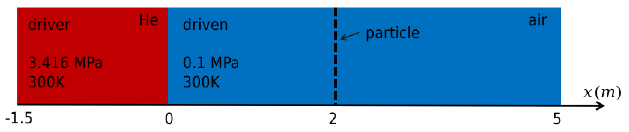
3.1. Shock–Particle Curtain Interaction

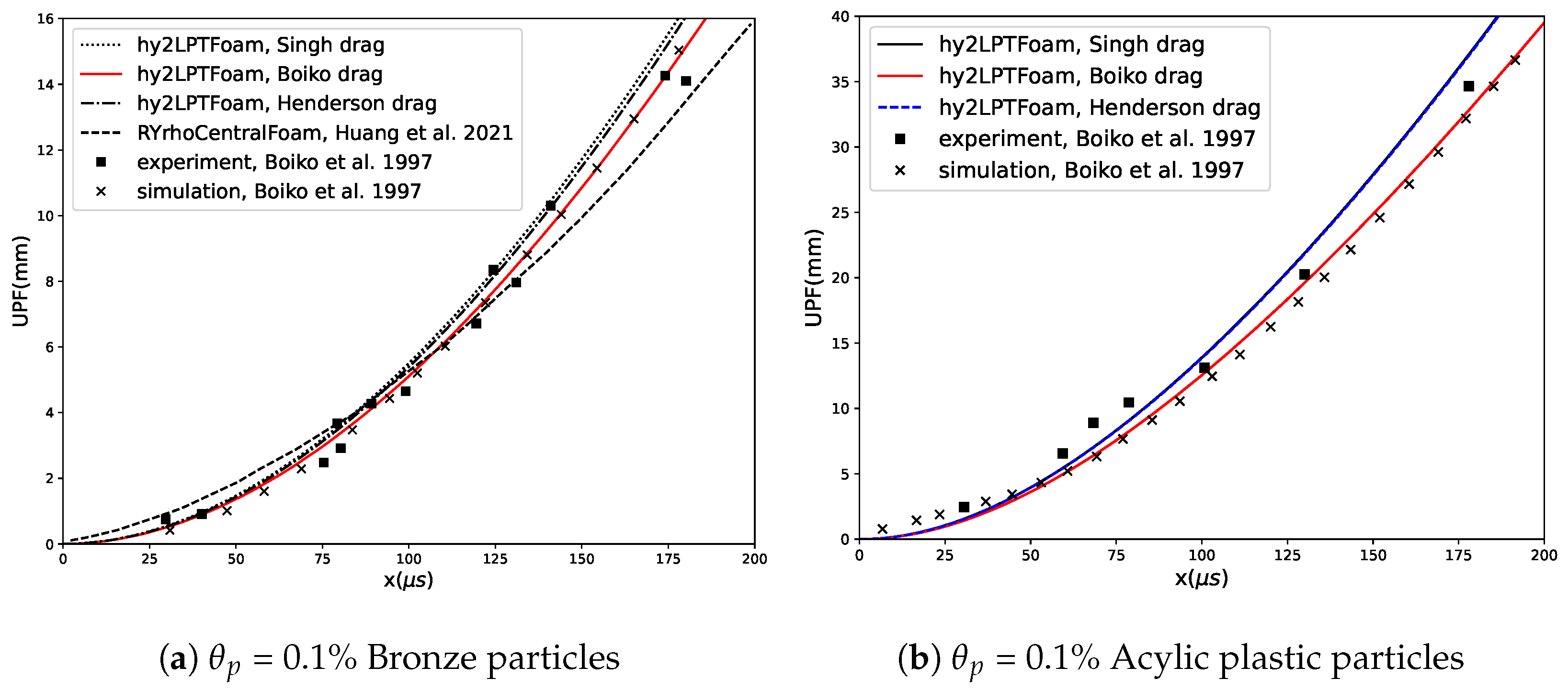
3.1.1. Low Particle Volume Fraction

A verification test based on the shock–particle interaction experiment conducted by Boiko et al. [35] was carried out. In this experiment, the computational domain is a 6.5 m long shock tube consisting of a 1.5 m driver section and a 5 m driven section, as described by Boiko et al. in [35]. Although the experiment exhibits three-dimensional effects, the shock wave is treated as one-dimensional in this numerical test. Particles with a volume fraction of 0.1% are initialized at $x=2$ m. The initial pressures in the driver and driven sections are 3.416 MPa and 0.1 MPa, respectively, and the temperature is 300 K, as depicted in Figure 6. This initial condition yields a shock Mach number of 2.8. The driven section is filled with air, while the driver section is filled with helium.

The comparison in Figure 7 shows the upstream particle front (UPF), identified as the leftmost particle location, between the simulation results and the experiment [35] and the numerical results from RYrhoCentralFoam [16]. Bronze particles with a density of 8600 kg/m³ and a diameter of 130 $\mathsf{\mu }$m are used in Figure 7a, while Figure 7b shows results using acrylic plastic particles with a density of 1200 kg/m³ and a diameter of 300 $\mathsf{\mu }$m. Three different drag models are used to calculate the UPF. The results obtained using the drag model in [35] match well with the numerical results in [35], with negligible discrepancies. There is no significant difference between the results obtained with the Singh [28] and Henderson [33] drag models; the particle movements using these two drag models are both longer than those using the Boiko [35] drag model. Compared with the Boiko [35] drag correlation, the Singh [28] and Henderson [33] drag models are based on consideration of the Mach number effect and the rarefaction effect. Hence, the UPFs acquired with the Singh [28] and Henderson [33] drag models agree better with the experiment results.

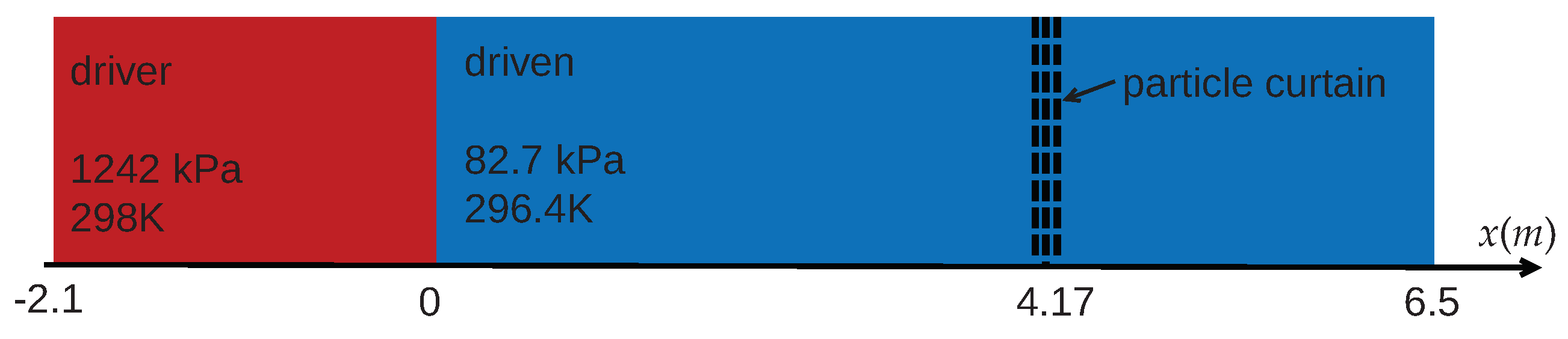
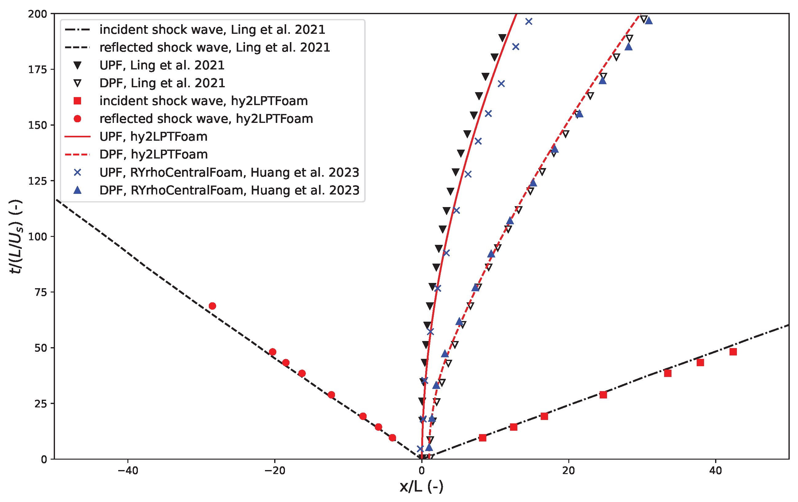
3.1.2. Moderate Particle Volume Fraction ${\theta }_p$ = 21%

In Section 3.1.1, it was unnecessary to consider particle–particle collisions due to the low solid volume fraction. However, when the solid volume fraction is increased to a moderate level of 21%, particle–particle collisions become an important factor in the evolution of the two-phase flow.

The simulation here, based on the work of Ling et al. [49], is about the interaction of a shock wave with a dense particle curtain, as shown in Figure 8. The problem is simplified by neglecting the three-dimensional effects and focusing on a one-dimensional computational domain. The cell size is 2 × ${10}^{-4}$ m. The gas in the shock tube is composed of 77% N₂ and 23% O₂, with a respective pressure and temperature of 1242 kPa and 298 K in the driver section and 82.7 kPa and 296.4 K in the driven section. The solid particles have a density of 2520 kg/m³ and a diameter of 1.15 × ${10}^{-4}$ m. The drag force is calculated using the Gidaspow [27] drag model (Ergun–Wen–Yu [50]). The particle–particle interaction is modeled using the MPPIC method with the Harris and Crighton model, in which

$${\tau }_p={\displaystyle \frac{P_s{\theta }_p^{\beta }}{max[{\theta }_{cp}-{\theta }_p,ϵ(1-{\theta }_p)]}},$$

(37)

where ${\theta }_{cp}$ is 0.6, $P_s$ is $8\times {10}^5$, $\beta$ is 3, $ϵ$ is $1\times {10}^{-7}$, and the coefficient of restitution is 0.9. The time step used in the simulation is 2 × ${10}^{-8}$ s.

Figure 9 presents the comparison of the upstream particle front and the downstream particle front (DPF, the rightmost particles) from te experiment and hy2LPTFoam. The results prove that the new solver can accurately predict the transmitted and reflected shock waves and the particle movement in supersonic flows. The particle UPFs and DPFs are in good agreement with both the experimental data [49] and RYrhoCentralFoam [17].

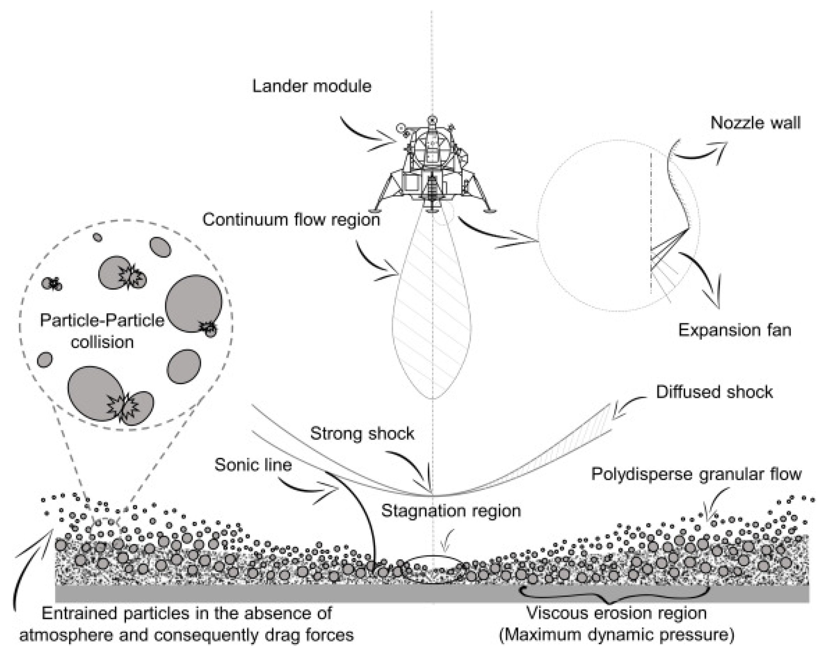
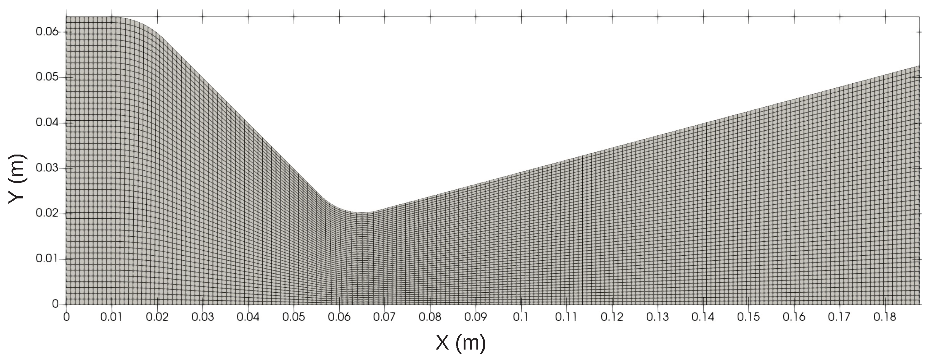
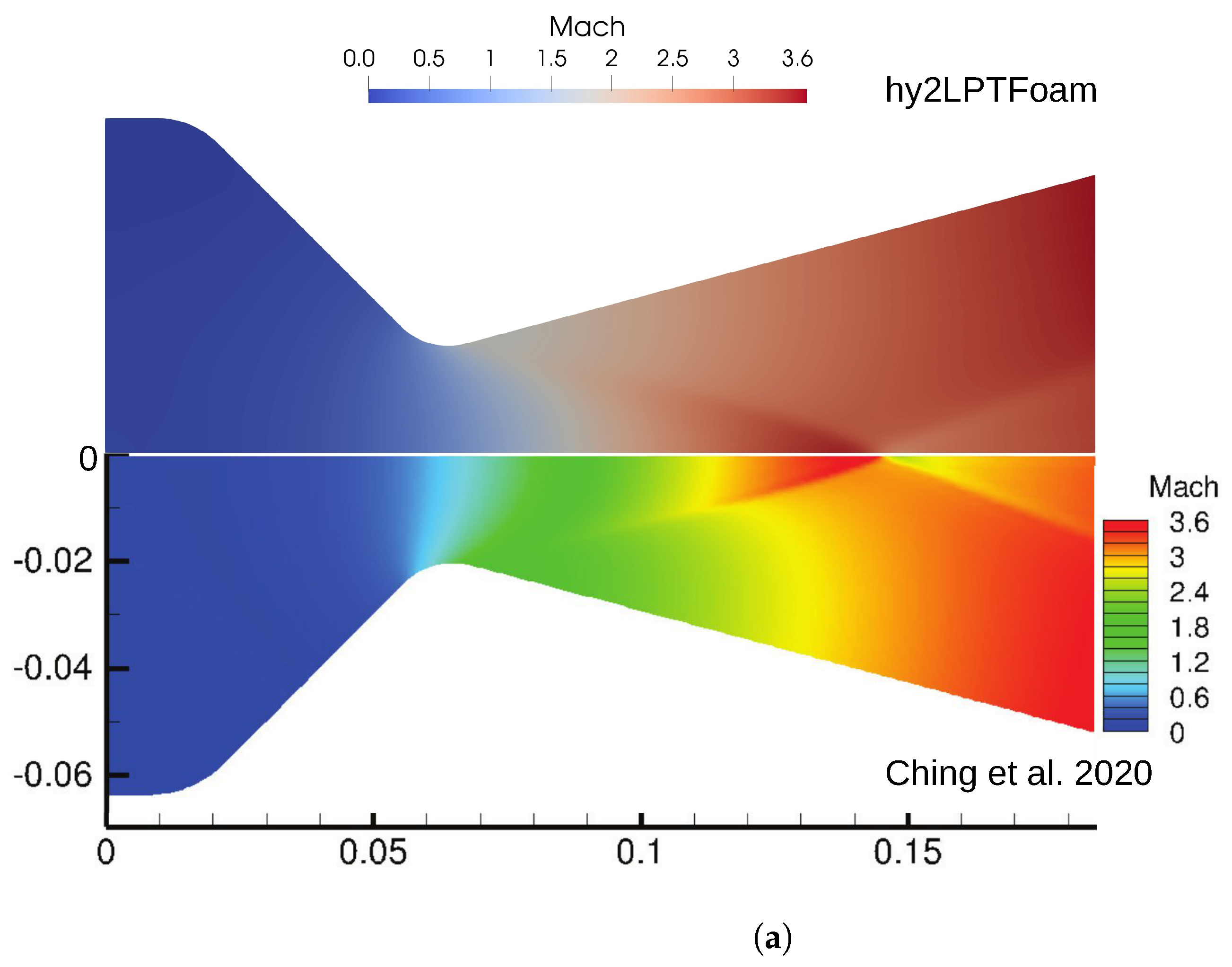
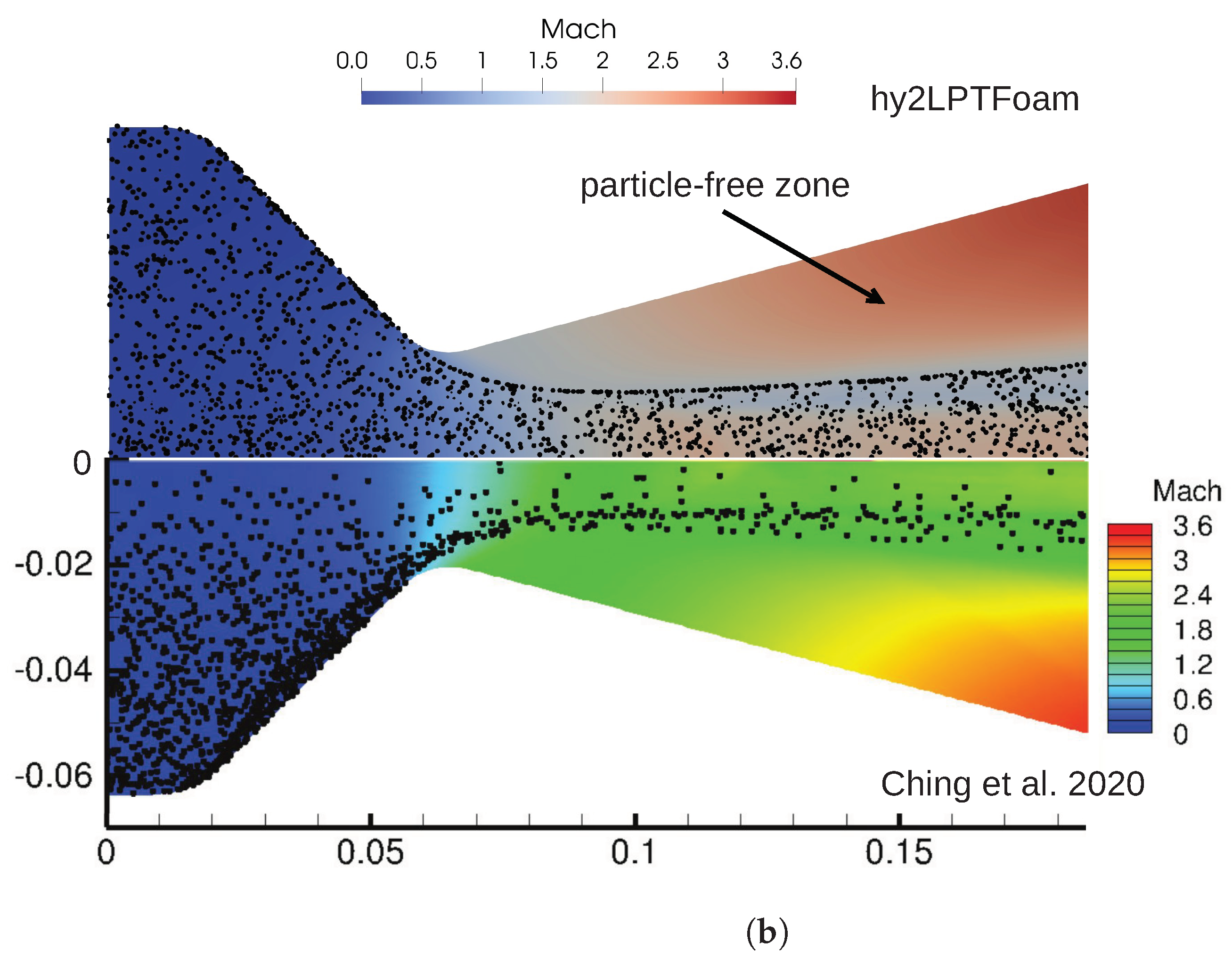
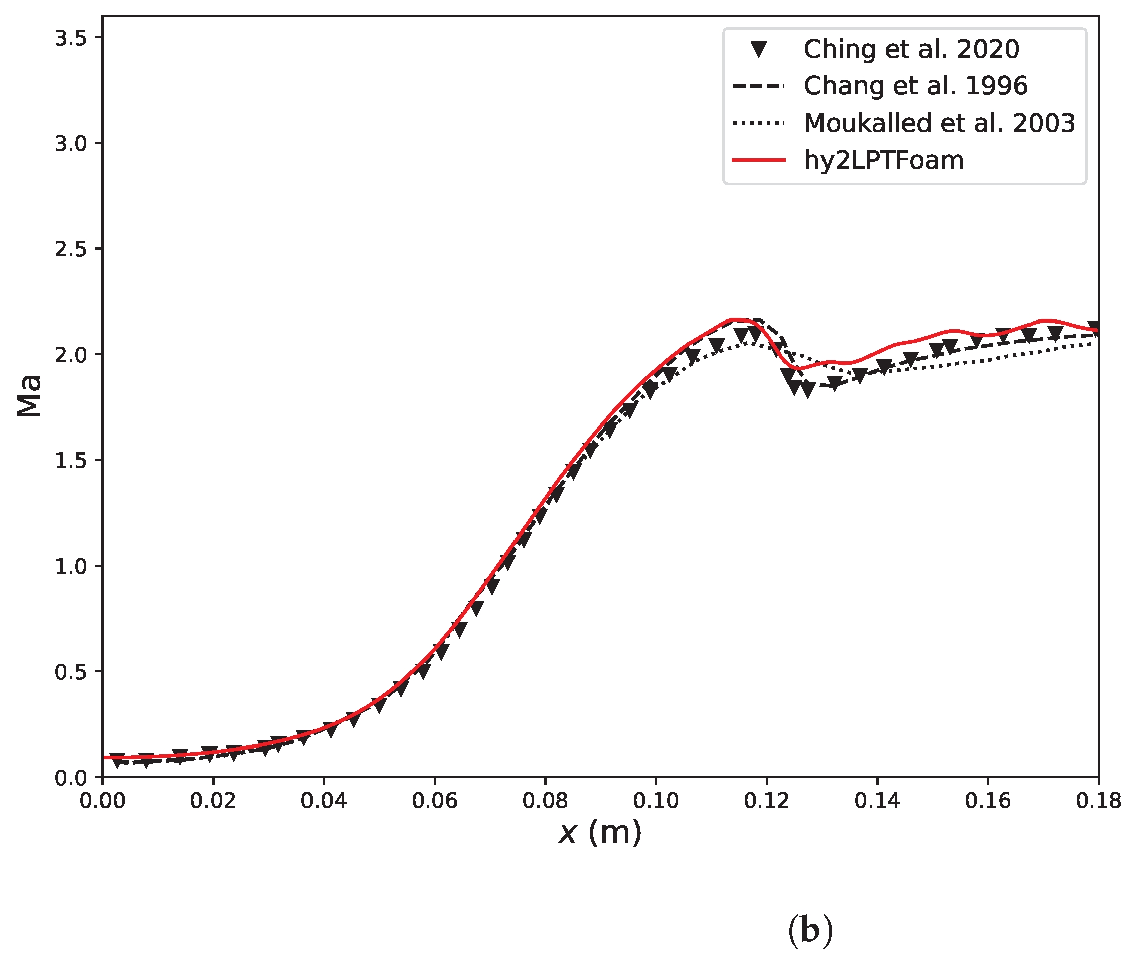
3.2. Two-Phase Flow in JPL Thruster

The “JPL” thruster has been widely studied in the validation of supersonic gas flow solvers [13,18,51,52] and gas–particle two-phase flows [18,52,53]; however, only experiments with pure gas exist [54]. hy2LPTFoam was used to repeat this two-way coupling for a two-phase flow.

The details of the geometry information for the JPL nozzle can be found in [53]. The computation is carried out using a 190 × 50 (x × y) structured axisymmetric mesh; see Figure 10.

Concerning the boundary conditions, the total pressure and total temperature boundary conditions are used at the inflow surface. The wedge boundary condition in OpenFOAM is implemented at the front and back wedge surfaces. The nozzle wall is adiabatic and slip for the gas phase, meaning that no boundary layer is generated near the wall. The particle phase experiences specular reflection when it hits the nozzle wall, meaning that there is no kinetic energy loss due to particle–wall collisions.

The flow conditions are provided in

Table 1. Flow conditions of the two-phase flow in the JPL nozzle.

gas total pressure (Pa)	1.034 × ${10}^4$
gas total temperature (K)	555
particle specific heat capacity (J/kg/K)	1380
particle density (kg/m3)	4004.62
particle diameter (m)	2 × ${10}^{-7}$
particle inflow mass fraction	0.3

. The simulation involves a gas mixture of nitrogen and oxygen, with mass fractions of 77% for $N_2$ and 23% for $O_2$. The particles injected from the inlet boundary are assumed to be in equilibrium with the gas phase, meaning that their initial velocity and temperature are equal to the gas velocity and temperature.

The drag coefficient is modeled according to [35] as proposed by Clift and Gauvin; see Equation (22). The Nusselt number is calculated based on Equation (31).

The steady state of the gas phase is acquired before injecting any particles. Excellent agreement is found in the Mach number field (see Figure 11a) and Mach number distribution at the nozzle axis (see Figure 11a) between the results from hy2LTPFoam and those from the literature [18,52,54]. The gas continues to accelerate after being injected into the nozzle. The flow reaches the speed of sound at the throat and forms a weak oblique shock in the divergent part. This shock wave extends downstream and touches the nozzle axis. The gas decelerates after passing through the shock wave and starts a new acceleration.

Based on Figure 11a and Figure 12b, it can be seen that the particles injected into the nozzle have a significant impact on the flow field. Because the particles are assumed to be in equilibrium with the gas phase, they continue to absorb momentum and heat from the gas phase as they travel through the nozzle. With a particle diameter of 20 microns, the particles do not respond quickly to the gas flow, creating a particle-free zone in the divergent section of the nozzle, as shown in Figure 11b.

It should be mentioned that particle-free zone becomes significantly smaller when the particle diameter is 2 microns [52,53]. The Mach distribution shown in Figure 12b is time-averaged due to fluctuation caused by the relatively low number of particles in the axisymmetric mesh. The Mach distribution from hy2LPTFoam demonstrates good agreement with previous results in the literature. In comparison with the Mach number distribution in Figure 12a, it is evident that the peak Mach number along the axis decreases from 3.5 to 2.1. This reduction in the peak Mach number results in a decrease in shock wave strength and a shift in its location upstream from $x=0.14$ m (Figure 12a) to $x=0.12$ m (Figure 12b).

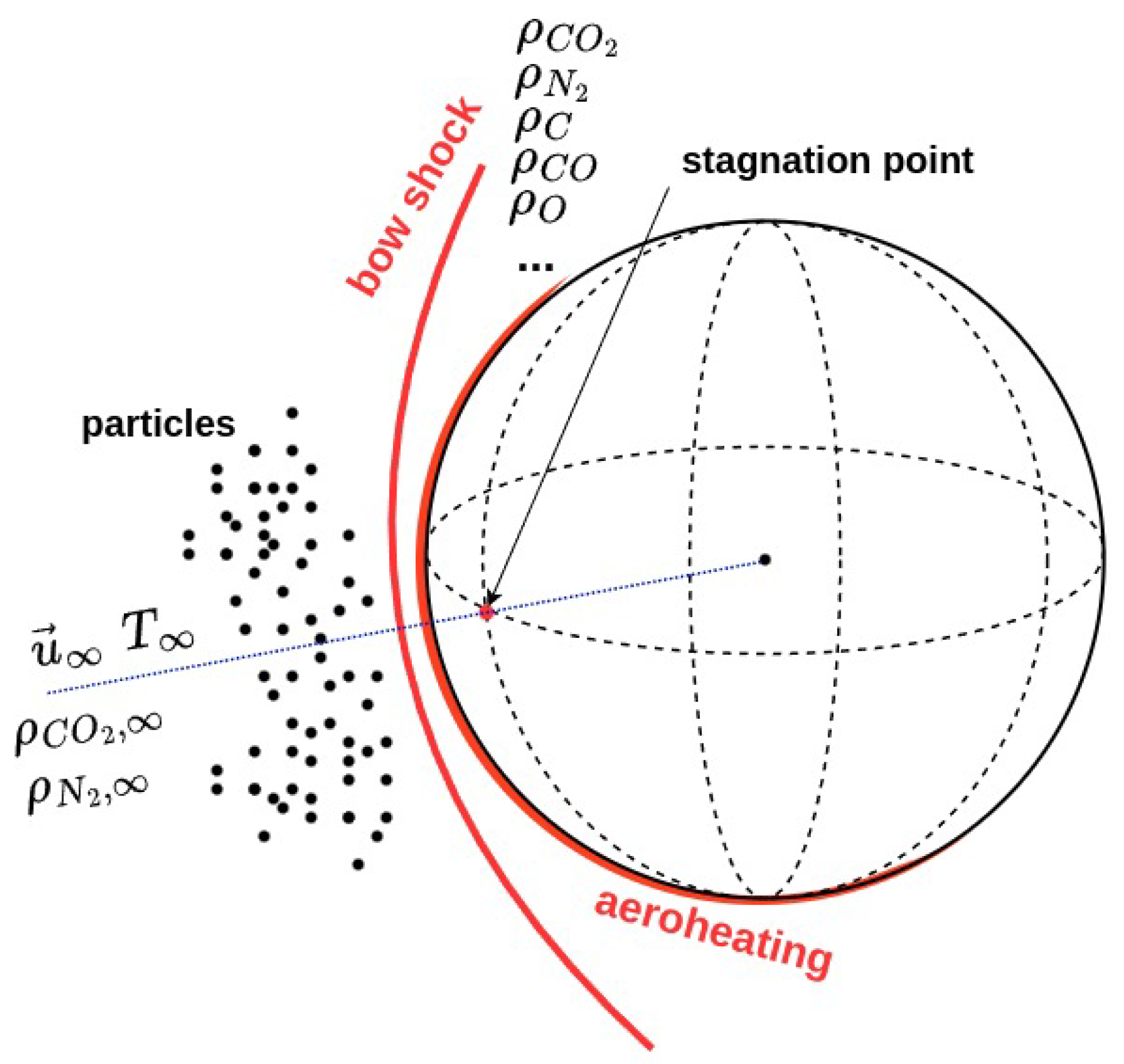
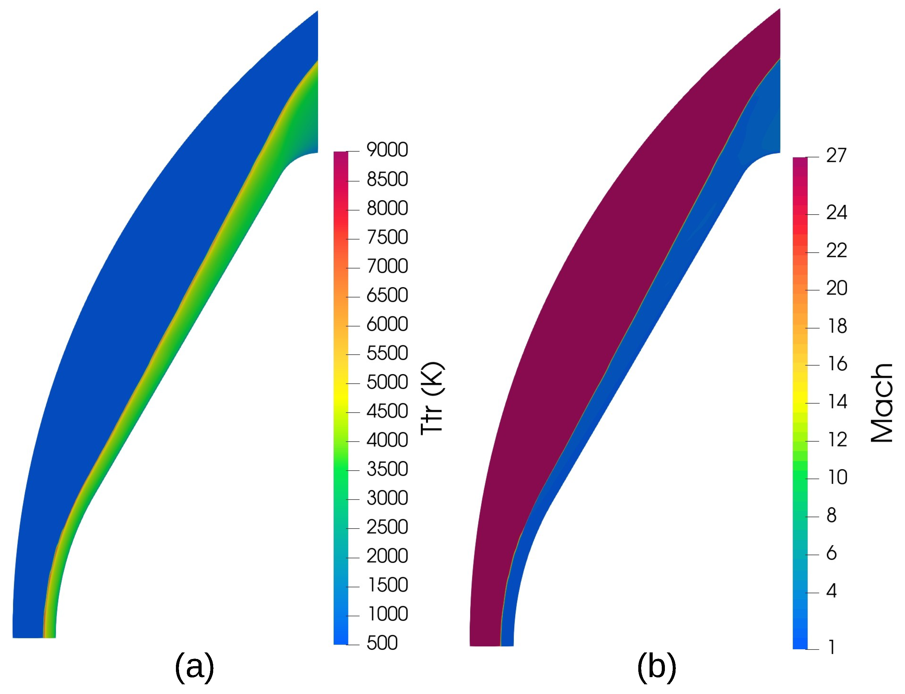
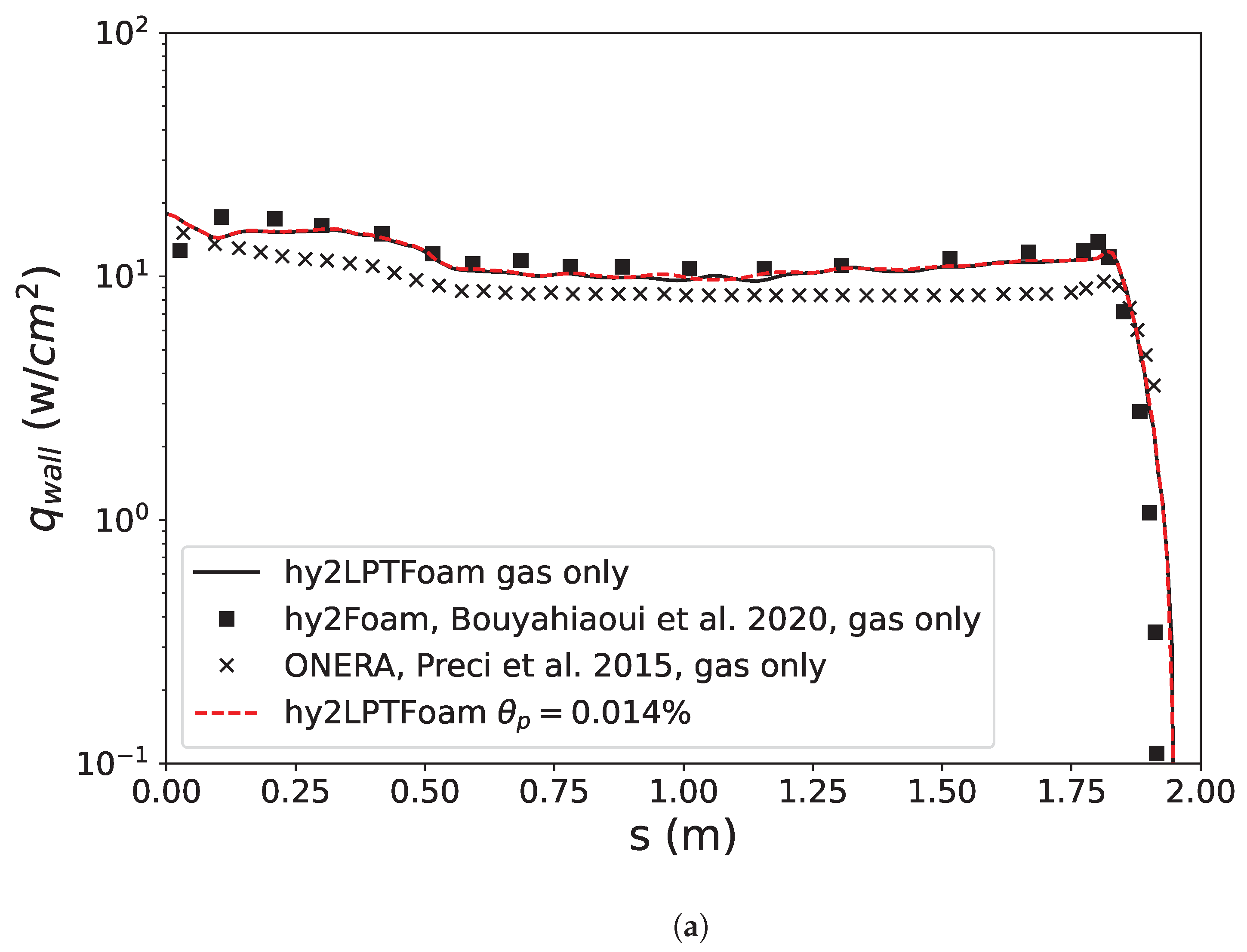
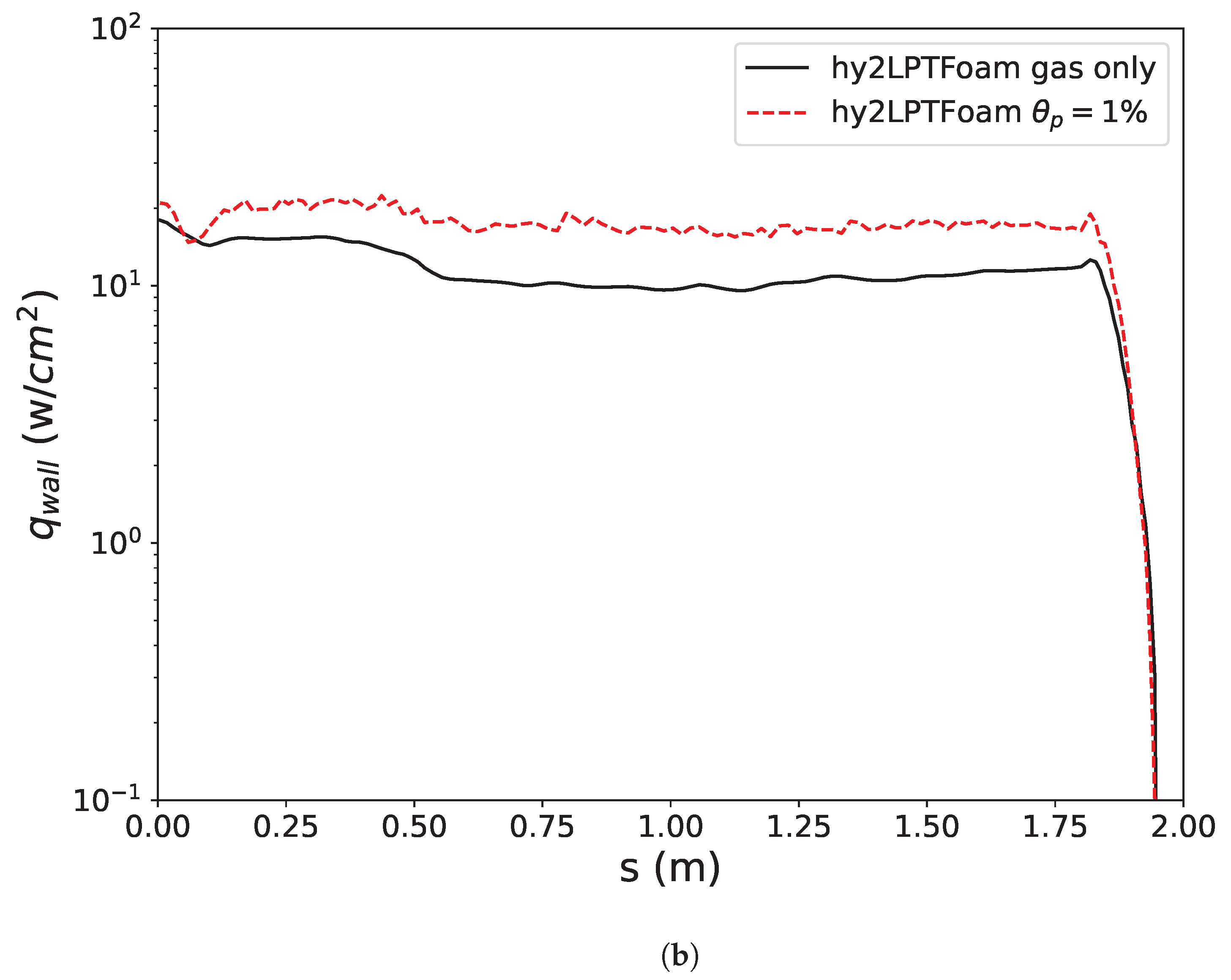
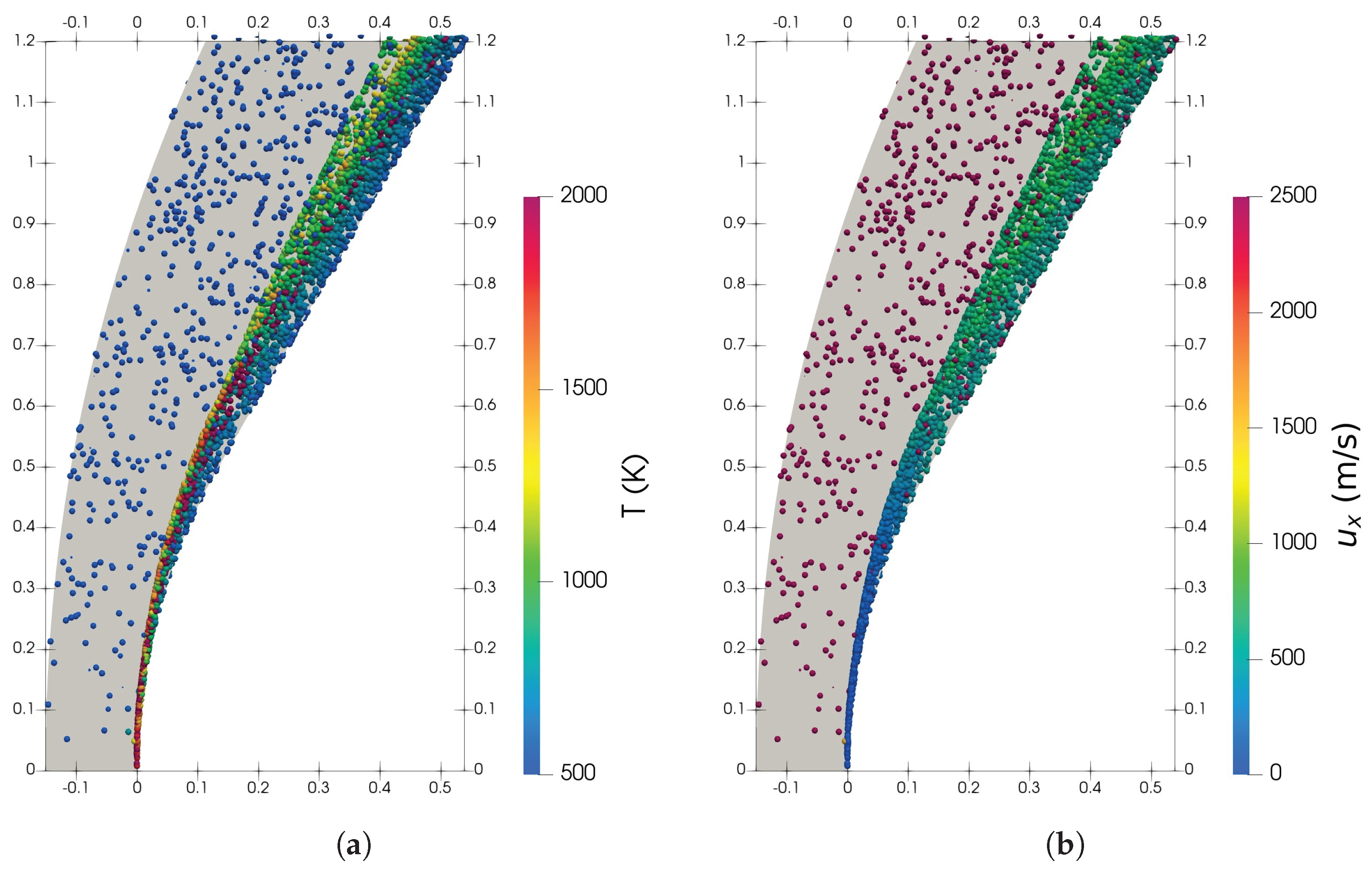
3.3. MSRO Body: Hypersonic Non-Equilibrium Flow during Mars Entry

The flow around an entry body during the Mars atmospheric entry process is a typical example of hypersonic non-equilibrium two-phase flow, in this case due to the possibility of sandstorms on Mars. The two-phase flow of Test Case 3 (TC-3) of the MSRO body has been previously studied in [55,56], and is repeated here using hy2LPTFoam with $0°$ angle of attack.

The Mars Sample Return Orbiter (MSRO) is a $60°$ sphere-cone with a nose cap of radius 1 m and a shoulder of radius 0.15 m [57], see Figure 13. The calculation of the geometry profile of the entry body can be found in [58]. A $61\times 260$ structured axisymmetric mesh with clusters at the boundary layer of the MSRO body surface and the shock wave is implemented in the test case.

The details of the simulation parameter are presented in

Table 2. Flow conditions of the TC3.

Wall Condition	Non-Catalytic
$C{O}_2$ mass fraction	1.0
Wall temperature	1500
Gas velocity (m/s)	5223
Pressure (Pa)	7.87
Temperature (K)	140
particle density (kg/m3)	2940
particle diameter (m)	$2.5\times {10}^{-6}$
particle specific heat capacity (J/kg/K)	1000

. The simulation considers five gas species: $C{O}_2$, $O_2$, $CO$, O, and C, along with the dissociation and exchange reactions listed in

Table 3. Forward and backward reaction coefficients of the Arrhenius law; M is gas molecule and A is gas atom.

Reaction	${\mathit{A}}_{\mathit{f}}$	${\mathit{B}}_{\mathit{f}}$	${\mathbf{\Theta }}_{\mathit{f}}$	${\mathit{A}}_{\mathit{b}}$	${\mathit{B}}_{\mathit{b}}$	${\mathbf{\Theta }}_{\mathit{b}}$
$C{O}_2+M\iff CO+O+M$	$6.9\times {10}^{18}$	−1.5	63,275	$1.14\times {10}^8$	−0.75	535
$C{O}_2+A\iff CO+O+A$	$1.38\times {10}^{19}$	−1.5	63,275	$2.28\times {10}^8$	−0.75	535
$CO+M\iff C+O+M$	$2.3\times {10}^{17}$	−1.0	129,000	$5.13\times {10}^9$	−1.0	0
$CO+A\iff C+O+A$	$3.4\times {10}^{17}$	−1.0	129,000	$7.59\times {10}^9$	−1.0	0
$O_2+M\iff O+O+M$	$2.0\times {10}^{18}$	−1.5	59,500	$2.0\times {10}^9$	−1.0	0
$O_2+A\iff O+O+A$	$1.0\times {10}^{19}$	−1.5	59,500	$1.0\times {10}^{10}$	−1.0	0
$CO+CO\iff C{O}_2+C$	$2.33\times {10}^6$	0.5	65,710	$4.6\times {10}^9$	−0.25	0
$CO+O\iff O_2+C$	$3.9\times {10}^{10}$	−0.18	69,200	$1.34\times {10}^{11}$	−0.43	0
$C{O}_2+O\iff O_2+CO$	$2.1\times {10}^{10}$	0	27,800	$4.011\times {10}^7$	0.5	23,800

. The viscosity of the gas species is calculated based on [59]. The mixing rule provided by Armaly and Sutton [60] is used to calculate the gas mixture quantities. The energy exchange between the trans-rotational and vibro-electronic energy modes (V-T) is evaluated using the Landau–Teller equation [61]. The V-T relaxation time is calculated using the semi-empirical formula by Millikan and White [62], with the Park correction relation [3] included due to the high temperature in the simulation. Additionally, the Park TTv chemistry–vibration coupling model is applied.

The Henderson drag model (Equations (19) and (20)) and the Kavanau Nusselt number correlation (Equations (32) and (33)) have been implemented. It is assumed that the contact heat transfer in the calculation of energy exchange at the wall is negligible. Additionally, it is suggested that the kinetic energy lost by the particle due to collision is absorbed by the wall through heat transfer [63]. The heat flux of particles to the sphere wall is then calculated as follows:

$$q_{coll,w}={\displaystyle \frac{1}{A_{cell}\Delta t}}\sum _{i=1}^{N_{coll,w}}(E_k-E_k^{\prime })$$

(38)

where $E_k=0.5m_p{\left|{\overrightarrow{v}}_p\right|}^2$ is the kinetic energy of the particles. When particles collide with the surface of the entry body, the coefficient of restitution needs to be taken into account in order to update the velocity after the collision. Tsirkunov et al. [64] developed a semi-empirical model for calculating the coefficient of restitution during collisions. The normal coefficient of restitution $a_n$ depends on the incident velocity and the incident angle $\beta$, while the tangential coefficient of restitution $a_t$ is influenced by various coefficients related to the materials of the wall and the particle. However, these coefficients are only suitable for certain materials, such as steel and copper [64]. As a result, the simulation only takes the normal coefficient of restitution into consideration, which is expressed as

$$a_n=1-[1-exp(-0.1|{\overrightarrow{v}}_p{|}^{0.61})]sin\beta .$$

(39)

Similar to Section 3.2, the steady state of the gas flow field is obtained before conducting two-phase simulations. The translational–rotational temperature and the Mach field are shown in Figure 14. As the gas crosses the shock wave, the translational–rotational temperature increases, while the Mach number decreases. This is followed by a decrease in the mass fraction of CO₂ and an increase in the mass fraction of the other gas species due to chemical reactions. The mass fractions of C, O₂, and O in Figure 15 are consistent with those found in [56]. The difference in mass fraction of CO₂ and CO can be attributed to the mesh near the wall and the number of cells in the y-direction, as the chemical and surface heat flux convergence are sensitive to the mesh. However, the surface heat flux of the pure gas phase in Figure 16a matches previous results at this mesh level, and the convergence of the surface heat flux is not the primary focus of this work. Therefore, the gas flow results at this mesh level will be used for further study of the two-phase cases.

In the two-phase simulations, two different particle mass fractions are studied: (a) 0.014% and (b) 1%. The simulations presented in Figure 17 show that the particles experience heating and deceleration shortly after passing through the bow shock. Specifically, near the stagnation point, the particle velocities drop to zero and their temperatures exceed 2000 K; meanwhile, particles located further from the stagnation line are heated to around 500–1000 K and decelerated to speeds of 500–1200 m/s. Due to the velocity component in the y-direction, particles at the stagnation point move upwards in the region between the bow shock and the entry body.

It has been observed that an increase in particle mass fraction leads to an increase in the surface heat flux on the entry body [29,65]. When the particle mass fraction is extremely low, there are no obvious changes in the surface heat flux variation, as shown in Figure 16a. However, when the particle mass fraction is increased to 1%, a significant increase in the surface heat flux can be observed before the shoulder part of the entry body, as shown in Figure 16b. This demonstrates that hy2LPTFoam can produce physical results for high-speed non-equilibrium two-phase flows.

4. Conclusions

In this paper, the hy2Foam high-speed non-equilibrium flow solver is coupled with the Lagrangian particle tracking algorithm in OpenFOAM, resulting in a new model named hy2LPTFoam. This new solver incorporates multiple particle drag models, heat transfer models, diffusion-based smooth methods, and the MPPIC method. A series of verification cases yielded good agreement with previous experimental and numerical studies from the literature. Application of the new solver to shock–particle curtain interaction demonstrated its ability to accurately predict particle movements in supersonic flows under both low and moderate particle volume fraction conditions. This was achieved using one-way coupling and particle–particle interaction for the case with moderate particle volume fraction. In a comparison using the two-phase JPL nozzle flow, hy2LPTFoam yielded good results employing a two-way coupling method. To further validate the effectiveness of the solver, a representative MSRO entry scenario was solved, confirming its ability to provide physical results under hypersonic non-equilibrium flow conditions. It was observed that an increase in the entry body surface heat flux corresponded to a rise in the particle inflow mass fraction. Overall, these results indicate that hy2LPTFoam is capable of solving high-speed non-equilibrium gas–particle flows covering a broad range of Mach numbers and Knudsen numbers.

References

1. Majid, A.; Bauder, U.; Herdrich, G.; Fertig, M. Two-Phase Flow Solver for Hypersonic Entry Flows in a Dusty Martian Atmosphere. J. Thermophys. Heat Transf. 2016, 30, 418–428. [Google Scholar] [CrossRef]
2. Rahimi, A.; Ejtehadi, O.; Lee, K.; Myong, R. Near-field plume-surface interaction and regolith erosion and dispersal during the lunar landing. Acta Astronaut. 2020, 175, 308–326. [Google Scholar] [CrossRef]
3. Park, C. Nonequilibrium Hypersonic Aerothermodynamics; Wiley: New York, NY, USA, 1989. [Google Scholar]
4. Wright, M.J.; Candler, G.V.; Bose, D. Data-Parallel Line Relaxation Method for the Navier-Stokes Equations. AIAA J. 1998, 36, 1603–1609. [Google Scholar] [CrossRef]
5. Gnoffo, P.A. An Upwind-Biased, Point-Implicit Relaxation Algorithm for Viscous, Compressible Perfect-Gas Flows; No. NASA-TP-2953; Hampton, VA, USA, 1990. Available online: https://ntrs.nasa.gov/citations/19900007726 (accessed on 9 August 2024).
6. Daiß, A.; Schöll, E.; Frühauf, H.H.; Knab, O. Validation of the uranus navier-stokes code for high-temperature nonequilibrium flows. In Proceedings of the 5th International Aerospace Planes and Hypersonics Technologies Conference, Munich, Germany, 30 November–3 December 1993; p. 5070. [Google Scholar]
7. Candler, G.V.; Johnson, H.B.; Nompelis, I.; Gidzak, V.M.; Subbareddy, P.K.; Barnhardt, M. Development of the US3D code for advanced compressible and reacting flow simulations. In Proceedings of the 53rd AIAA Aerospace Sciences Meeting, Kissimmee, FL, USA, 5–9 January 2015; p. 1893. [Google Scholar] [CrossRef]
8. Haoui, R. Physico-chemical state of the air at the stagnation point during the atmospheric reentry of a spacecraft. Acta Astronaut. 2011, 68, 1660–1668. [Google Scholar] [CrossRef]
9. Casseau, V. An Open-Source CFD Solver for Planetary Entry. Ph.D. Thesis, University of Strathclyde, Glasgow, UK, 2017. [Google Scholar]
10. Vatansever, D.; Celik, B. An open-source hypersonic solver for non-equilibrium flows. J. Aeronaut. Space Technol. 2021, 14, 35–52. [Google Scholar]
11. Gibbons, N.N.; Damm, K.A.; Jacobs, P.A.; Gollan, R.J. Eilmer: An open-source multi-physics hypersonic flow solver. Comput. Phys. Commun. 2023, 282, 108551. [Google Scholar] [CrossRef]
12. Bauder, U.; Fertig, M.; Auweter-Kurtz, M. Examination of the Coupling of the Loosely Coupled Sequential Navier-Stokes Code SINA. In Proceedings of the 40th Thermophysics Conference, Seattle, WA, USA, 23–26 June 2008; p. 3931. [Google Scholar]
13. Sahai, A.; Palmer, G. Variable-fidelity Euler–Lagrange framework for simulating particle-laden high-speed flows. AIAA J. 2022, 60, 3001–3019. [Google Scholar] [CrossRef]
14. Kroells, M.D.; Sahai, A.; Schwartzentruber, T.E. Sensitivity study of dust-induced surface erosion during Martian planetary entry. In Proceedings of the AIAA Scitech 2022 Forum, San Diego, CA, USA, 3–7 January 2022; p. 0112. [Google Scholar]
15. Greenshields, C.J.; Weller, H.G.; Gasparini, L.; Reese, J.M. Implementation of semi-discrete, non-staggered central schemes in a colocated, polyhedral, finite volume framework, for high-speed viscous flows. Int. J. Numer. Methods Fluids 2010, 63, 1–21. [Google Scholar] [CrossRef]
16. Huang, Z.; Zhao, M.; Xu, Y.; Li, G.; Zhang, H. Eulerian-Lagrangian modelling of detonative combustion in two-phase gas-droplet mixtures with OpenFOAM: Validations and verifications. Fuel 2021, 286, 119402. [Google Scholar] [CrossRef]
17. Zhang, P.; Zhang, H.; Zhang, Y.F.; Li, S.; Meng, Q. Modeling particle collisions in moderately dense curtain impacted by an incident shock wave. Phys. Fluids 2023, 35, 023327. [Google Scholar] [CrossRef]
18. Ching, E.J.; Brill, S.R.; Barnhardt, M.; Ihme, M. A two-way coupled Euler-Lagrange method for simulating multiphase flows with discontinuous Galerkin schemes on arbitrary curved elements. J. Comput. Phys. 2020, 405, 109096. [Google Scholar] [CrossRef]
19. Snider, D.M. An incompressible three-dimensional multiphase particle-in-cell model for dense particle flows. J. Comput. Phys. 2001, 170, 523–549. [Google Scholar] [CrossRef]
20. O’Rourke, P.J.; Snider, D.M. An improved collision damping time for MP-PIC calculations of dense particle flows with applications to polydisperse sedimenting beds and colliding particle jets. Chem. Eng. Sci. 2010, 65, 6014–6028. [Google Scholar] [CrossRef]
21. O’Rourke, P.J.; Snider, D.M. Inclusion of collisional return-to-isotropy in the MP-PIC method. Chem. Eng. Sci. 2012, 80, 39–54. [Google Scholar] [CrossRef]
22. Marayikkottu Vijayan, A.; Levin, D.A. Study of shock interaction with a particle curtain using the Multiphase Particle in Cell (MP-PIC) approach. In Proceedings of the AIAA SCITECH 2023 Forum, National Harbor, MD, USA, 23–27 January 2023; p. 0281. [Google Scholar]
23. Ranjbari, P.; Emamzadeh, M.; Mohseni, A. Numerical analysis of particle injection effect on gas-liquid two-phase flow in horizontal pipelines using coupled MPPIC-VOF method. Adv. Powder Technol. 2023, 34, 104235. [Google Scholar] [CrossRef]
24. Vincent, C.; Daniel, E.; Thomas, S.; Richard, B. A Two-Temperature Open-Source CFD Model for Hypersonic Reacting Flows, Part Two: Multi-Dimensional Analysis. Aerospace 2016, 3, 45. [Google Scholar] [CrossRef]
25. Cao, Z.; White, C.; Kontis, K. Numerical investigation of rarefied vortex loop formation due to shock wave diffraction with the use of rorticity. Phys. Fluids 2021, 33, 067112. [Google Scholar] [CrossRef]
26. Cao, Z.; White, C.; Agir, M.B.; Kontis, K. Lunar plume-surface interactions using rarefiedMultiphaseFoam. Front. Mech. Eng. 2023, 9, 1116330. [Google Scholar] [CrossRef]
27. Gidaspow, D. Multiphase Flow and Fluidization: Continuum and Kinetic Theory Descriptions; Academic Press: Cambridge, MA, USA, 1994. [Google Scholar]
28. Singh, N.; Kroells, M.; Li, C.; Ching, E.; Ihme, M.; Hogan, C.J.; Schwartzentruber, T.E. General drag coefficient for flow over spherical particles. AIAA J. 2022, 60, 587–597. [Google Scholar] [CrossRef]
29. Ching, E.J.; Singh, N.; Ihme, M. Simulations of Dusty Flows over Full-Scale Capsule During Martian Entry. J. Spacecr. Rocket. 2022, 59, 2053–2069. [Google Scholar] [CrossRef]
30. Habeck, J.B.; Kroells, M.D.; Schwartzentruber, T.E.; Candler, G.V. Characterization of particle-surface impacts on a sphere-cone at hypersonic flight conditions. In Proceedings of the AIAA SCITECH 2023 Forum, National Harbor, MD, USA, 23–27 January 2023; p. 0205. [Google Scholar]
31. Osnes, A.N.; Vartdal, M.; Khalloufi, M.; Capecelatro, J.; Balachandar, S. Comprehensive quasi-steady force correlations for compressible flow through random particle suspensions. Int. J. Multiph. Flow 2023, 165, 104485. [Google Scholar] [CrossRef]
32. Boniou, V.; Fox, R.O. Shock–particle-curtain-interaction study with a hyperbolic two-fluid model: Effect of particle force models. Int. J. Multiph. Flow 2023, 169, 104591. [Google Scholar] [CrossRef]
33. Henderson, C.B. Drag coefficients of spheres in continuum and rarefied flows. AIAA J. 1976, 14, 707–708. [Google Scholar] [CrossRef]
34. Clift, R.; Gauvin, W. Motion of Particles in Turbulent Gas Streams. Br. Chem. Eng. 1971, 16, 229. [Google Scholar]
35. Boiko, V.; Kiselev, V.; Kiselev, S.; Papyrin, A.; Poplavsky, S.; Fomin, V. Shock wave interaction with a cloud of particles. Shock Waves 1997, 7, 275–285. [Google Scholar] [CrossRef]
36. Loth, E. Compressibility and Rarefaction Effects on Drag of a Spherical Particle. AIAA J. 2008, 46, 2219–2228. [Google Scholar] [CrossRef]
37. Fox, T.W.; Rackett, C.W.; Nicholls, J.A. Shock wave ignition of magnesium powders. In Shock Tube and Shock Wave Research; Eleventh International Symposium. 1978. Available online: https://ntrs.nasa.gov/citations/19790031222 (accessed on 9 August 2024).
38. Carlson, D.J.; Hoglund, R.F. Particle drag and heat transfer in rocket nozzles. AIAA J. 1964, 2, 1980–1984. [Google Scholar] [CrossRef]
39. Tewfik, O.E. Discussion on G. C. Vliet and G. Leppert: ‘Forced convection heat transfer from an isothermal sphere to water’. J. Heat Transf. 1961, 83, 175. [Google Scholar] [CrossRef]
40. Kavanau, L.L. Heat transfer from spheres to a rarefied gas in subsonic flow. Trans. Am. Soc. Mech. Eng. 1955, 77, 617–623. [Google Scholar] [CrossRef]
41. Crowe, C.T.; Schwarzkopf, J.D.; Sommerfeld, M.; Tsuji, Y. Multiphase Flows with Droplets and Particles; CRC Press: Boca Raton, FL, USA, 2011. [Google Scholar]
42. Andrews, M.J.; O’Rourke, P.J. The multiphase particle-in-cell (MP-PIC) method for dense particulate flows. Int. J. Multiph. Flow 1996, 22, 379–402. [Google Scholar] [CrossRef]
43. Harris, S.; Crighton, D. Solitons, solitary waves, and voidage disturbances in gas-fluidized beds. J. Fluid Mech. 1994, 266, 243–276. [Google Scholar] [CrossRef]
44. Lun, C.K.; Savage, S.B.; Jeffrey, D.; Chepurniy, N. Kinetic theories for granular flow: Inelastic particles in Couette flow and slightly inelastic particles in a general flowfield. J. Fluid Mech. 1984, 140, 223–256. [Google Scholar] [CrossRef]
45. Are, S.; Hou, S.; Schmidt, D.P. Second-order spatial accuracy in Lagrangian–Eulerian spray calculations. Numer. Heat Transf. Part B 2005, 48, 25–44. [Google Scholar] [CrossRef]
46. Sun, R.; Xiao, H. Diffusion-based coarse graining in hybrid continuum–discrete solvers: Theoretical formulation and a priori tests. Int. J. Multiph. Flow 2015, 77, 142–157. [Google Scholar] [CrossRef]
47. Sun, R.; Xiao, H. Diffusion-based coarse graining in hybrid continuum–discrete solvers: Applications in CFD–DEM. Int. J. Multiph. Flow 2015, 72, 233–247. [Google Scholar] [CrossRef]
48. Zhang, J.; Li, T.; Ström, H.; Wang, B.; Løvås, T. A novel coupling method for unresolved CFD-DEM modeling. Int. J. Heat Mass Transf. 2023, 203, 123817. [Google Scholar] [CrossRef]
49. Ling, Y.; Wagner, J.; Beresh, S.; Kearney, S.; Balachandar, S. Interaction of a planar shock wave with a dense particle curtain: Modeling and experiments. Phys. Fluids 2012, 24, 113301. [Google Scholar] [CrossRef]
50. Zhou, L.; Zhang, L.; Bai, L.; Shi, W.; Li, W.; Wang, C.; Agarwal, R. Experimental study and transient CFD/DEM simulation in a fluidized bed based on different drag models. RSC Adv. 2017, 7, 12764–12774. [Google Scholar] [CrossRef]
51. Chang, H.T.; Hourng, L.W.; Chien, L.C.; Chien, L.C. Application of flux-vector-splitting scheme to a dilute gas–particle jpl nozzle flow. Int. J. Numer. Methods Fluids 1996, 22, 921–935. [Google Scholar] [CrossRef]
52. Moukalled, F.; Darwish, M.; Sekar, B. A pressure-based algorithm for multi-phase flow at all speeds. J. Comput. Phys. 2003, 190, 550–571. [Google Scholar] [CrossRef]
53. Maochang, D.; Xijun, Y.; Dawei, C.; Fang, Q.; Shijun, Z. Numerical Simulation of Gas-Particle Two-Phase Flow in a Nozzle with DG Method. Discret. Dyn. Nat. Soc. 2019, 2019, 7060481. [Google Scholar] [CrossRef]
54. Cuffel, R.; Back, L.; Massier, P.F. Transonic flowfield in a supersonic nozzle with small throat radius of curvature. AIAA J. 1969, 7, 1364–1366. [Google Scholar] [CrossRef]
55. Preci, A.; Auweter-Kurtz, M. Sensitivity analysis of non-equilibrium martian entry flow to chemical and thermal modelling. In Proceedings of the 53rd AIAA Aerospace Sciences Meeting, Kissimmee, FL, USA, 5–9 January 2015; p. 0982. [Google Scholar]
56. Bouyahiaoui, Z.; Haoui, R.; Zidane, A.; Nouiri, A. Prediction of the flow field and convective heating during space capsule reentry using an open source solver. Int. J. Heat Mass Transf. 2020, 148, 119045. [Google Scholar] [CrossRef]
57. Surzhikov, S.T. TC3: Convective and radiative heating of MSRO for simplest kinetic models. In Proceedings of the Radiation of High Temperature Gases in Atmospheric Entry, Porquerolles, France, 30 September–1 October 2004; Volume 583, p. 55. [Google Scholar]
58. Prabhu, D.; Saunders, D. On heatshield shapes for Mars entry capsules. In Proceedings of the 50th AIAA Aerospace Sciences Meeting including the New Horizons Forum and Aerospace Exposition, Nashville, TN, USA, 9–12 January 2012; p. 399. [Google Scholar]
59. Blottner, F.G.; Johnson, M.; Ellis, M. Chemically Reacting Viscous Flow Program for Multi-Component Gas Mixtures; Technical report; Sandia National Lab. (SNL-NM): Albuquerque, NM, USA, 1971.
60. Armaly, B.; Sutton, K. Viscosity of multicomponent partially ionized gas mixtures. In Proceedings of the 15th Thermophysics Conference, Snowmass, CO, USA, 14–16 July 1980; p. 1495. [Google Scholar]
61. Landau, L. Theory of sound dispersion. Phys. Z. Der Sowjetunion 1936, 10, 34–43. [Google Scholar]
62. Millikan, R.C.; White, D.R. Systematics of vibrational relaxation. J. Chem. Phys. 1963, 39, 3209–3213. [Google Scholar] [CrossRef]
63. Oesterle, B.; Volkov, A.N.; Tsirkunov, Y.M. Numerical investigation of two-phase flow structure and heat transfer in a supersonic dusty gas flow over a blunt body. Prog. Flight Phys. 2013, 5, 441–456. [Google Scholar]
64. Tsirkunov, Y.M.; Panfilov, S.; Klychnikov, M. Semiempirical model of impact interaction of a disperse impurity particle with a surface in a gas suspension flow. J. Eng. Phys. Thermophys. 1994, 67, 1018–1025. [Google Scholar] [CrossRef]
65. Hinkle, A.; Hosder, S.; Johnston, C. Efficient Two-Way Coupled Analysis of Steady-State Particle-Laden Hypersonic Flows. J. Spacecr. Rocket. 2024, 61, 48–60. [Google Scholar] [CrossRef]
Figure 1. Schematic of Mars entry during a sandstorm.
Aerospace 11 00742 g001
Figure 2. Schematic of plume–surface interactions [2].
Aerospace 11 00742 g002
Figure 3. Solver flow chart.
Aerospace 11 00742 g003
Figure 4. An example of diffusion-based smoothing of the particle volume fraction.
Aerospace 11 00742 g004
Figure 5. The particle volume fraction distribution along the line at the center of the domain in Figure 4; b is the bandwidth, whie the number of steps is the number of diffusion steps in OpenFOAM.
Aerospace 11 00742 g005
Figure 6. Computational domain of the shock–particle interaction with low solid volume fraction.
Aerospace 11 00742 g006
Figure 7. The upstream particle front variation under the conditions of different particle material [16,35].
Aerospace 11 00742 g007
Figure 8. Computational domain of the shock–particle interaction with moderate solid volume fraction.
Aerospace 11 00742 g008
Figure 9. Comparison of experimental and numerical results from hy2LPTFoam: normalized x–t diagram [17,49].
Aerospace 11 00742 g009
Figure 10. Mesh of the JPL thruster.
Aerospace 11 00742 g010
Figure 11. JPL Mach number field. (a): Pure gas; (b): Two-phase [18].
Aerospace 11 00742 g011aAerospace 11 00742 g011b
Figure 12. Mach number distribution at the centerline of the JPL thruster in two-phase condition [18,51,52,54].
Aerospace 11 00742 g012aAerospace 11 00742 g012b
Figure 13. Schematic of TC3 body geometry and mesh.
Aerospace 11 00742 g013
Figure 14. Flow field of TC3 body: (a) translational-rotational temperature and (b) Mach number.
Aerospace 11 00742 g014
Figure 15. Distribution of gas species along the stagnation line [56].
Aerospace 11 00742 g015
Figure 16. TC3 body surface convective heat flux distribution; s is the curve along the entry body [55,56].
Aerospace 11 00742 g016aAerospace 11 00742 g016b
Figure 17. Temperature and velocity component in the x direction of particles. (a,b): θ p = 0.014 % ; (c,d): θ p = 1 % .
Aerospace 11 00742 g017aAerospace 11 00742 g017b