A Low Earth Orbit Satellite-Orbit Extrapolation Method Based on Multi-Satellite Ephemeris Coordination and Multi-Stream Fractional Autoregressive Integrated Moving Average

Abstract

The low Earth orbit (LEO) satellite internet network (LEO-SIN) has become a heated issue for the next generation of mobile communications, serving as a crucial means to achieve global wide-area broadband coverage and, especially, mobile phone directly to satellite cell (MPDTSC) communication. The ultra-high-speed movement of LEO satellites relative to the Earth results in serious Doppler effects, leading to signal de-synchronization at the user end (UE), and relative high-speed motion leading to frequent satellite handovers. Satellite ephemeris, which indicates the satellite’s position, has the potential to determine the position of the transmit (Tx) within the LEO-SIN, thereby enhancing the reliability and efficiency of satellite communication. The adoption of ephemeris in the LEO-SIN has met some new challenges: (1) how UEs can acquire ephemerides before signal synchronization is complete, (2) how to minimize the frequency of ephemeris broadcasting, and (3) how to decrease the overhead of ephemeris broadcasting. To address the above challenges, this paper proposes a method for extrapolating the LEO-SIN orbit based on multi-satellite ephemeris coordination (MSEC) and the multi-stream fractional autoregressive integrated moving average (MS-FARIMA). First, a multi-factor global error analysis model for ephemeris-extrapolation error is established, which decomposes it into three types; namely, random error (RE), trending error (TE), and periodic error (PE), with a focus on increasing the extrapolation accuracy by improving RE and TE. Second, RE is eliminated by utilizing the ephemerides from multiple satellites received at the same UE at the same time, as well as multiple ephemerides from the same satellite at different times. Subsequently, we propose a new FARIMA algorithm with the innovation of a multi-stream data time-series forecast (TSF), which effectively improves ephemeris extrapolation errors. Finally, the simulation results show that the proposed method reduces ephemeris extrapolation errors by 33.5% compared to existing methods, which also contributes to a performance enhancement in the Doppler frequency offset (DFO) estimation of MPDTSC.

1. Introduction

An important element of the vision of sixth generation (6G) mobile communication is the achievement of global wide-area broadband communication, satisfying the demand for reliable and efficient communication services in areas such as mountains, oceans, deserts, and rural regions [1]. The low Earth orbit (LEO) satellite internet network (LEO-SIN) is one of the important solutions. Terrestrial-based mobile communication systems primarily serve users through a base station (BS), utilizing a communication model of fixed BSs and moving users. In this model, a cell handover can be determined by measuring the quality of the received BS signal power [2,3]. Unlike terrestrial-based mobile communication systems, the mobile phone directly to satellite cell (MPDTSC) concept utilizes a model with a high-speed moving satellite and a moving user. This means that even if the user remains motionless, the beams of the satellite covering the user will move rapidly, frequently requiring the user to select an appropriate new satellite and implement the handover to its beam in order to maintain continuous and reliable communication [4,5].

Based on the orbits of satellites within constellations and their ephemerides, users can predict which satellites will serve them in these corresponding locations, thereby supporting the selection of suitable satellites for access. Here, the ephemeris directly conveys the information on the positions and velocities of these satellites within LEO-SIN. This information can contribute to the estimation of the Doppler frequency offset (DFO), which is used to compensate for and resist the satellite channel response degradations [6,7]. Additionally, the ephemeris can be used to calculate the remaining time the satellite serves as a contact point to help with radio resource control (RRC), random access (RA), and hybrid automatic repeat requests (HARQs) [8]. In the case of an orbital altitude of about 300~1200 km with a minimum elevation angle of 30°, each satellite in orbit can serve a user for approximately 3~10 min, implying that the orbit extrapolation error must not be higher than 20 m.

The existing research on orbit extrapolation relies on modeling based on astrodynamics, which describes characteristics related to the satellite’s orbit and position, such as inclination, right ascension of the ascending node, eccentricity, and mean anomaly. However, due to the influence of uncertain constraints like Earth’s gravitational effects, the gravitational effects of other celestial bodies, satellite attitude deviations, and ephemeris transmission errors, the real positions and velocities of satellites would be different from the values of the extrapolation, and this difference would gradually enlarge with time [9,10].

There are two schemes used to optimize the performance of orbit extrapolation; namely, increasing the frequency of ephemeris broadcasting and measurements, and performing interpolation calculations. As for the first scheme, its prerequisite is that the link between the satellite and the UE must already be established; otherwise, the UEs cannot receive any data, including the ephemeris. This would be relevant in the case of the UE’s initial access to a network or when the UE needs to re-access the network due to channel response degradation. Further, frequent ephemeris transmission requires extra overhead and radio resources, which decrease the efficiency of frequency utilization [11]. Additionally, increased measurement also requires an extensive number of ground stations (GSs) to continuously monitor the satellites, but this transmission is always much later than the time in which the UEs are in use [12]. In the latter scheme, interpolation is quite suitable in the case of limited ephemeris information and limited access to a referenced relative accurate location. Some algorithms such as Lagrange interpolation, Newton interpolation, and Chebyshev polynomial fitting can be used in orbit extrapolation improvement. The accuracy of interpolation methods depends on the accuracy of the boundary points of the observed ephemeris value and the interval of the interpolation [13,14]. In recent years, with the development of artificial intelligence (AI) algorithms, orbit extrapolation algorithms based on neural networks or deep learning have also gained a significant amount of attention. These methods primarily learn the uncertain errors of orbit extrapolation by measurements and fitting [15,16].

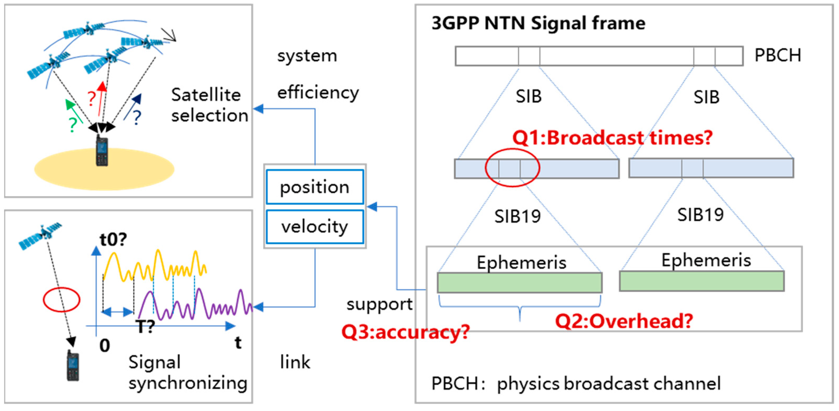
Based on the above analysis, the expected orbit extrapolation of the LEO-SIN needs to satisfy the following requirements, as shown in Figure 1: (1) the time of satellite ephemeris broadcasting should be limited, given the limited radio communication resources; (2) the outdated referenced ephemeris measured by GSs should be avoided, and (3) the accuracy of orbit extrapolation must improve. In our view, orbit extrapolation error is composed of distinct types of errors; if these errors can be separated, the total error would be expected to improve. Under the premise of the limited time for ephemeris broadcasting, the determination of adjacent satellites’ ephemeris information and the different timings of ephemeris information would be also expected to contribute to its enhanced performance.

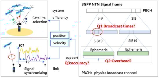
Figure 1. The role of the ephemeris and its challenges in the LEO-SIN.

Here, we explore novel research on orbit extrapolation methods based on multi-satellite ephemeris coordination (MSEC) and the multi-stream fractional autoregressive integrated moving average (MS-FARIMA). The main contributions can be summarized as follows.

• This work is the first to propose separating the broadcast ephemeris extrapolation errors into three types: random error (RE), trending error (TE), and periodic error (PE). It focuses on improving the extrapolation accuracy by diminishing and compensating for the RE and TE. We also derive the lower bound of the orbit extrapolation error based on single-satellite ephemeris information;
• This work first proposes a novel and accurate ephemeris extrapolation framework that involves the ephemerides of multi-satellite and multi-stream data time-series forecasting (TSF). By analyzing the spatial and temporal associations between corresponding and different satellites at different times, an MSEC orbit extrapolation error elimination algorithm can be designed. This algorithm utilizes multiple types of ephemeris information from MSEC to diminish the RE;
• This work is the first to design an MS-FARIMA algorithm, which supports data of the same attribute information at different times and of different objects. By applying the MS-FARIMA method, the accuracy of ephemeris error extrapolation is enhanced. Additionally, the reasons for the improved accuracy of the ephemeris extrapolation error based on MSEC and multi-stream information are explored;
• This work proposes a DFO estimation and compensation algorithm for the LEO-SIN based on the employment of the optimized ephemeris. It theoretically derives the impacts of different ephemeris errors on DFO estimation, enhancing the DFO estimation accuracy.

The remainder of this paper is organized as follows: Section 2 introduces related research on existing satellite ephemeris extrapolation methods, Section 3 constructs the ephemeris extrapolation system model for the LEO-SIN then models and analyzes single-satellite ephemeris extrapolation errors, Section 4 presents the MS-FARIMA algorithm and applies it to improve the ephemeris extrapolation accuracy, Section 5 provides a simulation analysis and refines the algorithm, applying the optimized algorithm to the DFO error compensation, and Section 6 presents the conclusions.

2. Related Works

Existing and related methods for orbit extrapolation mainly rely on the increased frequency of ephemeris broadcasting and complex interpolation calculations. They include three methods: analytical orbit extrapolation (AOE), polynomial fitting orbit extrapolation (PFOE), and dynamic model orbit extrapolation (DMOE).

In the research on AOE methods, M. Thammawichai et al. (2023) proposed a nonlinear programming model for orbit prediction based on the two-line element (TLE) set, showing that this model achieves better orbit prediction accuracy compared to the standard Keplerian and simplified general perturbation 4 (SGP4) models [17]. H. Ge et al. (2024) exploited the Chebyshev extrapolation to maintain the continuity of clock accuracy in the real-time global navigation satellite system (GNSS), which could reduce the root mean square error (RMSE) of the along-track, cross-track, and radial errors in real-time LEO orbits from 5.40, 4.70, and 7.33 cm to 5.18, 4.55, and 5.99 cm, respectively [18].

In the research on PFOE methods, K. Wang et al. (2023) obtained real-time LEO satellite orbits based on batch least squares and short-term prediction. Using real data from the GRACE C satellite at 500 km and the Sentinel-3B satellite at 810 km, the orbit error range was obtained as 2–4 cm [19]. They employed a set of known satellite orbit data to solve the polynomial coefficients, which fit the polynomials via methods such as Chebyshev curve fitting, Lagrange interpolation, and least squares.

In the research on DMOE methods, Y. Zhuang et al. (2023) employed a broadcast ephemeris and GRACE D data for LEO’s 10-day real-time dynamic orbit determination, achieving a three-dimensional root mean square (3D-RMS) of 72.8 cm for GRACE D over 10 days [20]. This work was based on known satellite trajectory data and used dynamic analysis to calculate the satellite’s initial position, velocity, and other dynamic parameters for orbit prediction.

In summary, the primary format for a satellite-transmitted ephemeris is the two-line element (TLE), which records the six Keplerian orbital elements (SKOEs) of the satellite’s motion. The PFOE method is greatly influenced by the fitting time and the selection of the polynomial order, making it difficult to balance the fitting time and accuracy. The extrapolation accuracy of the DMOE method is highly dependent on the initial state parameters and the chosen dynamic model; if the initial state parameters are not well selected, the prediction accuracy cannot meet the requirements. On the other hand, the AOE method has the advantages of simplicity, a low computational load, and the ability to predict orbits without numerical integration.

Due to the Earth’s gravitational effects, the gravitational effects of other celestial bodies, satellite attitude deviations, and ephemeris transmission errors, large errors occur in satellite orbit prediction when using the existing methods. To better eliminate the errors, the LEO-SIN orbit extrapolation method based on MSEC and MS-FARIMA decomposes the extrapolation error into RE, TE, and PE, enabling significant improvements in accuracy and efficiency.

3. System Model and Problem Formulation

3.1. System Model

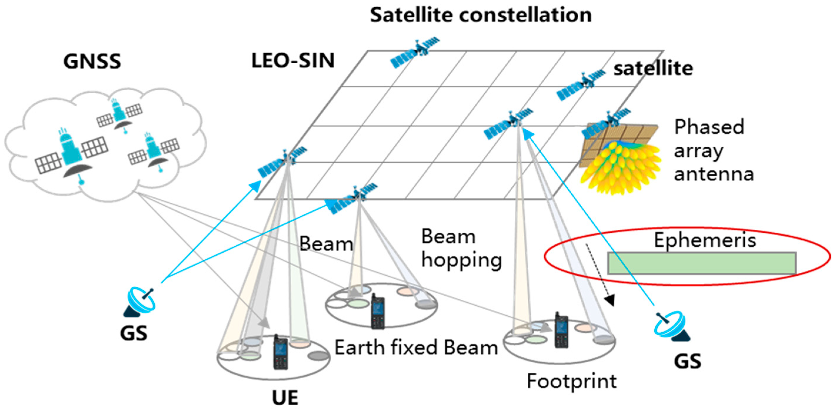
In the LEO-SIN, UEs receive ephemeris information not only from the current serving satellite at an observed time, but also from all visible satellites within the UE’s line-of-sight (LOS) coverage at that moment and some previous moments, as shown in Figure 2. The following information can support orbit extrapolation performance enhancement: the ephemeris for the same satellite at different times, the ephemeris for adjacent satellites at the same time, and the correlation between the broadcast ephemeris and relatively accurate ephemeris for the same satellite. The analysis and use of this information is expected to further improve the ephemeris extrapolation errors.

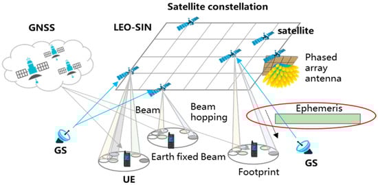
Figure 2. System model of LEO-SIN.

We assume a three-parameter set $\{\mathrm{T}, \mathrm{P}, \mathrm{F}\}$ to define a Walker constellation, where $\mathrm{T}$ is the total number of satellites in the constellation, $\mathrm{P}$ is the number of orbital planes, and $\mathrm{F}$ is the phase factor, which is an integer ranging from 0 to $\mathrm{P}-1$. The phase difference $\Delta {\phi }_i$ between satellites with the same number in different orbital planes is determined by the phase factor $\mathrm{F}$ and can be expressed as

$$\Delta {\phi }_i={\displaystyle \frac{2\pi }{\mathrm{T}}}\times \mathrm{F}, \mathrm{F}=0,1,2,3,\cdots ,\mathrm{P}-1$$

(1)

The phase difference between satellites with the same number in the $\mathrm{P}-1$ and 0th orbital planes is given by

$$\Delta {\phi }_{P-1}=(\mathrm{P}-1)\Delta {\phi }_1$$

(2)

For a given orbital altitude, the orbital inclination, the initial position of the seed satellite, and the three-parameter set $\{\mathrm{T}, \mathrm{P}, \mathrm{F}\}$ uniquely determines a Walker constellation.

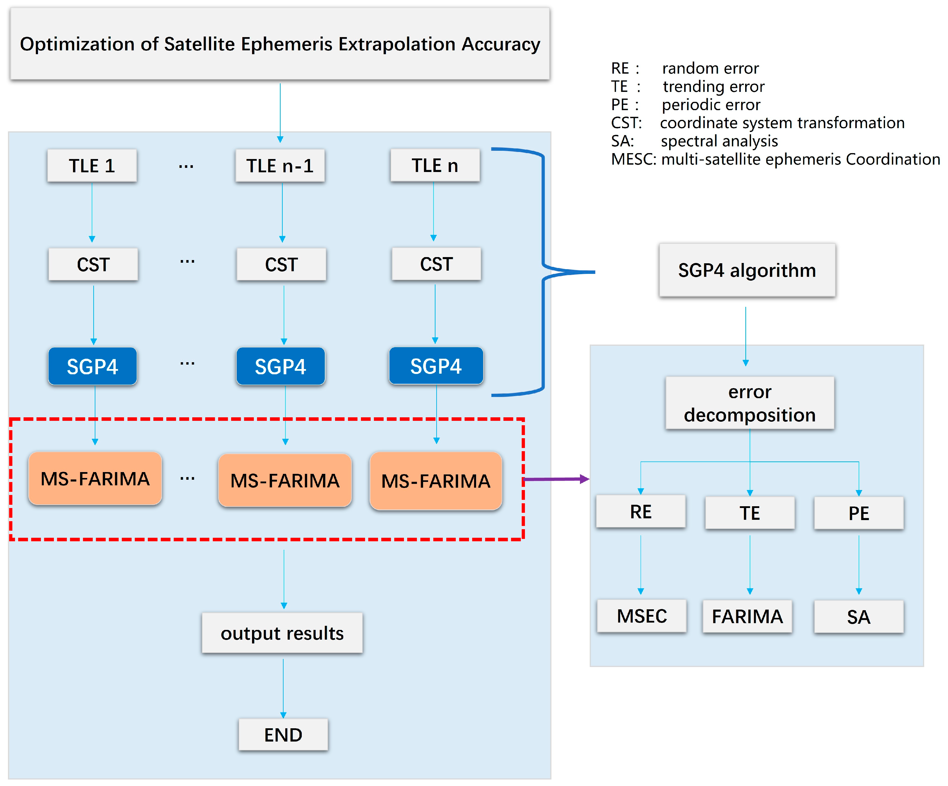
In this work, a series of related satellites within the UE’s LOS coverage will be analyzed. These satellites form a group of satellites, which consists of satellites with the same orbit or adjacent orbits within the same constellation. Each satellite periodically broadcasts its ephemeris in TLE format to the UEs, while the GSs periodically send measured and calculated accurate ephemeris data to the satellites. Figure 3 illustrates the scenario of satellite monitoring, ephemeris calculation, and broadcasting.

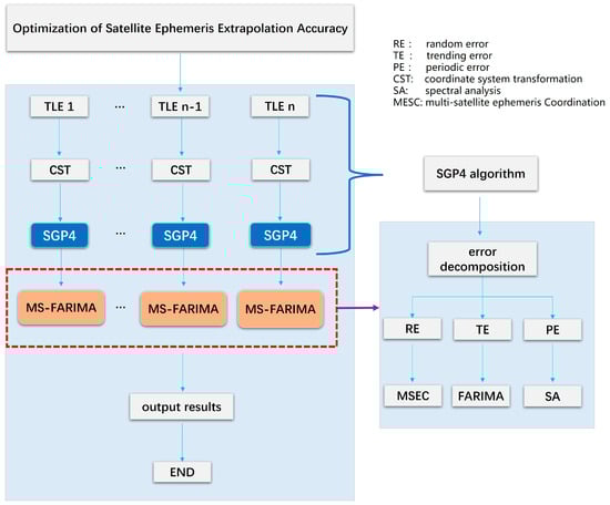
Figure 3. The flowchart of the proposed method.

We assume that a UE is considered in the satellite footprint, which can simultaneously receive ephemeris information from multiple different satellites. Orbit extrapolation with different satellites’ ephemerides exhibits different levels of accuracy. At a given time $t$, the corresponding ephemeris can be denoted as ${\mathbb{E}}_{\mathbb{L},\mathbb{t},\mathbb{S}}$, where $\mathbb{L}$ denotes the UE LOS area, which is typically the region covered by the satellite signals. Here, $\mathbb{L}=\{{\mathcal{L}}_0,{\mathcal{L}}_1,\dots ,{\mathcal{L}}_N\}$, where $N$ is the number of beam footprints of the serving satellite and ${\mathcal{L}}_i$ represents the $i\mathrm{th}$ beam footprint. $\mathbb{t}$ is the set of times at which TLE data are received in region $\mathbb{L}$, defined as $\mathbb{t}=\{{\mathcal{T}}_{{\mathcal{L}}_0},{\mathcal{T}}_{{\mathcal{L}}_1},\dots ,{\mathcal{T}}_{{\mathcal{L}}_N}\}$. $\mathbb{S}$ is the set of correlated satellites, which is defined as $\mathbb{S}=\{S_0,S_1,\dots ,S_K\}$.

The set of ephemeris data ${\mathcal{T}}_{{\mathcal{L}}_i,t}$ received by the UE at position ${\mathcal{L}}_i$ at time $t$ is given by

$${\mathcal{T}}_{{\mathcal{L}}_i,t}=\left\{T_{{\mathcal{L}}_i,t,1}:T_{{\mathcal{L}}_i,t,K}\right\}$$

(3)

where K is the number of correlated satellites and $T_{{\mathcal{L}}_i,t,K}$ represents the ephemeris data of satellite K received by the UE in this service area at the time $t$.

The proposed method, aimed at multi-satellite ephemeris extrapolation, can effectively improve the extrapolation accuracy. Figure 3 shows the flowchart of the proposed method.

The left side of the flowchart represents the overall process of optimizing the satellite’s ephemeris extrapolation accuracy. The right side provides a detailed description of the proposed MS-FARIMA algorithm, including error decomposition and the specific methods used to eliminate each type of error.

3.2. Problem Formulation

3.2.1. TLE Data

According to the recommendations of the third generation Partnership Project Non-Terrestrial Network (3GPP NTN), the two types of satellite ephemeris consist of SKOE data and data on the position and velocity. SKOE data are more widely exploited, particularly in the TLE format in system information block 19 (SIB19) [21,22]. SKOE data include the mean motion $n$, mean inclination $i$, mean eccentricity $e$, mean anomaly $M$, argument of periapsis $\omega$, and the mean longitude of the ascending node $\Omega$.

The TLE of the SKOEs describes the characteristics of the satellite’s ephemeris in the form of two lines with 70 columns each. The first line records basic information such as the satellite’s name and launch time. The second line records the parameters of the satellite’s operational orbit, which play the main role in orbit extrapolation. The details of the second line of the TLE table are shown in Table 1.

Table 1. The second line of TLE data.

Sequence Number	Digit Positions	Data Meaning
1	01–01	Line number
2	03–07	Satellite number
3	09–16	Inclination
4	18–25	Mean longitude of the ascending node
5	27–33	Eccentricity
6	35–42	Argument of periapsis
7	44–51	Mean anomaly
8	53–63	Number of revolutions per day
9	64–68	Number of orbits since launch
10	69–69	Checksum

As Table 1 shows, the TLE data reflect the mean orbital parameters using the true equator and mean equinox (TEME) expression, filtering out short-term perturbations.

Figure 4 illustrates the parameters of the TLE data. The SGP4 algorithm uses the TLE data to calculate the SKOEs to the position r and velocity $\dot{\mathit{r}}$ of the satellite in the TEME coordinate system [23,24]. Here, the TLE ephemeris in the TEME coordinate system should convert the Earth-centered Earth-fixed (ECEF) coordinate system into X, Y, and Z coordinates as a function of time. The conversion formulas are as follows:

$${\left(\begin{array}{c}X\\ Y\\ Z\end{array}\right)}_{TOD}=R_z(\Delta \phi \cos ϵ)\left(\begin{array}{c}X\\ Y\\ Z\end{array}\right)$$

(4)

where $R_z\left(\Delta \phi \cos ϵ\right)$ is the rotation matrix used to convert the position vector from the TEME coordinate system to the ECEF coordinate system. $R_z$ denotes the rotation matrix around the z-axis, $\Delta \phi$ denotes the Earth’s rotation angle due to the change in time, and $\cos ϵ$ represents the cosine of the angle between the equatorial plane and the ecliptic plane.

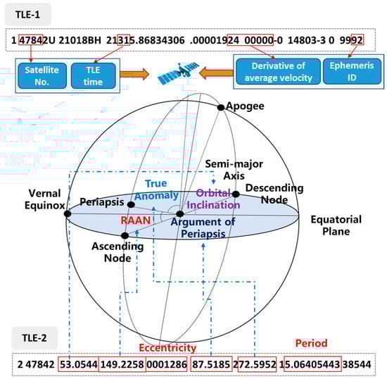
Figure 4. Parameters of TLE data mapping to the Earth.

3.2.2. Error Analysis of Orbit Extrapolation Based on Ephemeris

In the MPDTSC system, satellites’ ephemeris data are periodically broadcast to the UE in TLE format. The expected SGP4 model extrapolates the orbit to calculate the satellite’s location and velocity, with certain errors being caused by the Earth’s gravitational effects, the gravitational effects of other celestial bodies, satellite attitude deviations, and ephemeris transmission errors [25]. This error can be decomposed into three directional components in the spatial Cartesian coordinate system.

• Radial component R: the direction along the line connecting the satellite and the Earth’s center;
• Along-track component A: the tangential component within the orbital plane, perpendicular to the radial direction and pointing in the direction of the satellite’s motion;
• Cross-track component C: the component perpendicular to the orbital plane.

The broadcast ephemeris information received by the UE is denoted as ${\mathit{eph}}_{\mathit{broadcast}}$, and is in the form of TLE orbital elements:

$$\{n,i,e,M,\omega ,\mathsf{\Omega }\}$$

(5)

Based on the referenced time $t_{oe}$ and the orbital elements in the TLE ephemeris data, the SGP4 algorithm is used to extrapolate the following three-dimensional coordinate components of the position vector r:

$$\left[\begin{array}{c}x(n,i,\cdots ,\mathsf{\Omega },t_{oe},t)\\ y(n,i,\cdots ,\mathsf{\Omega },t_{oe},t)\\ z(n,i,\cdots ,\mathsf{\Omega },t_{oe},t)\end{array}\right]=\left[\begin{array}{c}x(P_t,t_{oe},t)\\ y(P_t,t_{oe},t)\\ z(P_t,t_{oe},t)\end{array}\right]$$

(6)

where $x(·)$, $y(·)$, $z(·)$ are the spatial position calculation functions of the satellite, which are the three-dimensional coordinate components of the position r calculated using the SGP4 algorithm. $P_t$ denotes the position at time t. The satellite’s broadcast ephemeris can be expressed as the sum of the real position and real velocity of the ephemeris ${ep\mathrm{h}}_0$ and the ephemeris error $\Delta \mathit{eph}$:

$$ep{h}_{broadcast}=ep{h}_0+\Delta eph$$

(7)

Unlike previous works that treat the orbit extrapolation error as a single error, we assume that there are multiple types of orbit extrapolation errors with different influencing factors.

$$\Delta eph(f_n(·))=\{\Delta eph(f_1(·)),\Delta eph(f_2(·)),\cdots ,\Delta eph(f_N(·))\}$$

(8)

where $\Delta eph\left(f_n\left(·\right)\right)$ denotes a set of orbit extrapolation errors with different influencing factors and $\Delta eph\left(f_N\left(·\right)\right)$ represents the n-th influencing factor.

3.2.3. Extrapolation Error of Single-Satellite Ephemeris

To analyze the lower bound of the orbit extrapolation error based on single-satellite ephemeris information, the observed function $\mathit{D}$ is defined. It denotes the operation of a time-series data process, consisting of the computation of a self-correlation with sliding window $l$ for any interval [0, $T_D$] sequentially. The results are a set of data $Z$, which is

$$Z=\{d_1,d_2,\cdots ,d_n\}$$

(9)

where $d_n$ represents the n-th group of data in the interval [0, $T_D$]. We separate the broadcast ephemeris extrapolation errors into three types: the RE, TE, and PE.

The RE consists of unpredictable noise in the ephemeris data due to various external and internal factors, such as satellite hardware limitations, signal interference, and environmental conditions. These errors do not follow a specific pattern and vary randomly over time. The TE arises due to the accumulation of systematic biases in the ephemeris data over time. These errors are usually caused by deficiencies in the satellite dynamics model, including gravitational influences and orbital perturbations, and they accumulate gradually as the satellite’s orbit continues. The PE is caused by the periodic nature of the satellite’s motion around the Earth. These errors are usually caused by the gravitational effects of celestial bodies, the oblateness of the Earth, and other periodic factors.

If the following conditions are met within $Z$

$$\forall d_i\in Z, d_i<d_t, i\ne n$$

(10)

this set of data time series can be considered to contain an RE $\Delta eph\left(\mathit{rand}\right)$. Here, $d_t$ in Equation (10) represents a threshold value. $\Delta eph\left(\mathit{rand}\right)$ affects all ephemeris orbit extrapolation errors received by the UE at the current moment.

If the following conditions are met within $Z$

$$\left\{\begin{array}{c}{d}_i\in Z,d_i>d_t,n\ne t\\ \forall d_i,d_j,d_i\ne d_j,i,j\le n\end{array}\right.$$

(11)

this set of data time series can be considered to contain a TE $\Delta eph\left(\mathit{trend}\right)$. $\Delta eph\left(\mathit{trend}\right)$ is caused by the characteristics of the SGP4 algorithm, in which ephemeris orbit extrapolation error is inevitable.

If the following conditions are met within $Z$

$$\left\{\begin{array}{c}{d}_i\in Z,d_i>d_t,n=t\\ d_1=d_2=\cdots =d_n\end{array}\right.$$

(12)

this set of time-series data can be considered to exhibit a PE $\Delta eph\left(\mathit{period}\right)$. $\Delta eph\left(\mathit{period}\right)$ is caused by the elliptical motion of the satellite around the Earth, where some errors periodically change with the movement of the satellite.

Then, we further separate these errors by defining three types of separation operators $\mathit{K}=\{K_1,K_2,K_3\}$. By orthogonally decomposing the extrapolation error component $\Delta eph\left(jt\right)$ with the three operators, the different orbit extrapolation errors can be separated:

$$\left\{\begin{array}{c}\mathit{K}·\Delta eph(rand)=(0,a,b)\\ \mathit{K}·\Delta eph(trend)=(a,0,b)\\ \mathit{K}·\Delta eph(period)=(a,b,0)\end{array}\right.$$

(13)

In Equation (13), $a$ and $b$ denote non-zero values.

3.2.4. Extrapolation Error Reduction in Single-Satellite Ephemeris

We simplify the orbit extrapolation error data as $S_{\mathit{orbit}}\left(t\right)$. Based on the previous analysis, since the ephemeris data exhibit certain long-term correlation characteristics, short-term correlation characteristics, and random characteristics, they can be decomposed into the RE component $U\left(t\right)$, PE component $S\left(t\right)$, and the TE component $R\left(t\right)$:

$$S_{orbit}(t)=U(t)+S(t)+R(t)$$

(14)

• Extraction and Processing of PE $S\left(t\right)$

For PE $S\left(t\right)$, due to its periodic characteristics, spectral analysis can be used to extract the PE from the ephemeris error $S_{\mathit{orbit}}\left(t\right)$. First, the fast Fourier transform (FFT) algorithm is used to convert the ephemeris extrapolation error from the time domain to the frequency domain, with the Fourier series expression of $\Delta \mathit{eph}$:

$$S_{orbit}(t)=A_0+{\displaystyle \sum _{i=1}^k(A_i\cos (2\pi {\omega }_{i}t)+B_i\sin (2\pi {\omega }_{i}t))}$$

(15)

where $A_0$ is the mean value of the extrapolation error over the observation period, $A_i$ and $B_i$ are the amplitudes of different PEs of the extrapolation error, and ${\omega }_i$ is the frequency of the corresponding PE. By utilizing the orthogonality of different PEs, it can be derived that

$$A_0={\displaystyle \frac{1}{T}}{\displaystyle \sum _{t=1}^T{S}_{orbit}(t)}$$

(16)

$$A_i={\displaystyle \frac{2}{T}}{\displaystyle \sum _{t=1}^T{S}_{orbit}(t)\cos (2\pi {\omega }_{i}t)}$$

(17)

$$B_i={\displaystyle \frac{2}{T}}{\displaystyle \sum _{t=1}^T{S}_{orbit}(t)\sin (2\pi {\omega }_{i}t)}$$

(18)

where $T$ represents the sampling period.

• Extraction and Processing of TE $R\left(t\right)$

TE $R\left(t\right)$ is caused by the characteristics of the SGP4 algorithm, which will gradually increase as the extrapolation time increases. Therefore, a TSF algorithm is exploited to learn the characteristics of the part of the data with small errors and predict subsequent data based on these characteristics.

We fit the upper and lower envelopes $\mathit{ul}\left(t\right)$ and $\mathit{dl}\left(t\right)$ of $S_{\mathit{orbit}}\left(t\right)$ based on all extrema of $S_{\mathit{orbit}}\left(t\right)$ and calculate their mean $\mathit{ml}\left(t\right)$. Then, we solve the trend characteristic function $g\left(t\right)=S_{\mathit{orbit}}\left(t\right)-\mathit{ml}\left(t\right)$. Depending on whether $g\left(t\right)$ is an intrinsic function, we iterate on $X_i\left(t\right)$ to obtain the intrinsic function $G_1\left(t\right)$. Next, we calculate the residual sequence $r_1\left(t\right)=S_{\mathit{orbit}}\left(t\right)-G_1\left(t\right)$. We repeat the above steps until $r_{n+1}\left(t\right)$ no longer meets the iterative conditions, forming the extracted trend component of $X_i\left(t\right)$:

$$S_{orbit}(t)={\displaystyle \sum _{i=1}^n{G}_i\left(t\right)}+r_{n+1}\left(t\right)$$

(19)

3.2.5. Communication Performance Influenced by Extrapolation Accuracy

High-speed relative motion causes a serious DFO in the LEO-SIN channel. By predicting the satellite’s position and velocity using ephemeris extrapolation algorithms, the DFO can be calculated and compensated for [26,27].

The DFO can be calculated using the traditional method as follows:

$$f_d=f_c{\displaystyle \frac{\left|{(v_{s\to u})}_{ecf}\right|}{v_c}}$$

(20)

where ${\left(v_{s\to u}\right)}_{\mathit{ecf}}$ denotes the velocity in the direction of the line connecting $R_u$ and $R_s$. It can be calculated that

$${(v_{s\to u})}_{ecf}={\displaystyle \frac{R_s·R_u}{‖R_s‖·‖R_u‖}}·S_v$$

(21)

where $S_v$ denotes the satellite’s velocity vector and $(R_u·R_s)/\left(\left|R_u\right|\left|R_s\right|\right)$ represents the cosine of the angle between the satellite and the UE.

According to Equation (4), the satellite’s position and velocity are obtained in the ECEF coordinate system over a given period. Let the position vector of the UE be $R_u$ = ${[X_U,Y_U,Z_U]}^T$, and the position vector of the satellite be $R_s$ = ${\left[X,Y,Z\right]}^T$.

Assume that the orthogonal frequency division multiplexing (OFDM) symbols transmitted from the satellite are received at the UE with a DFO ${\epsilon }_f$. The received signal $y\left[n\right]$ can be expressed as

$$y[n]=x[n]·e^{-{\displaystyle \frac{j2\pi {\epsilon }_{f}n}{N}}}$$

(22)

where $x\left[n\right]$ is the transmitted signal, $n$ ranges from 0 to $N-1$, and $N$ represents the number of subcarriers in one OFDM symbol.

Applying the FFT to the signal $y\left[n\right]$ converting to the frequency-domain signal $Y\left[k\right]$,

$$\begin{array}{l}Y[k]=FFT\{y[n]\}\\ ={\displaystyle \sum _{n=0}^{N-1}y[n]e^{-\frac{j2\pi kn}{N}}}\\ ={\displaystyle \frac{\sin (\pi {\epsilon }_f)}{N\sin (\frac{\pi {\epsilon }_f}{N})}}{e}^{-{\displaystyle \frac{j\pi {\epsilon }_f(N-1)}{N}}}X[k]+I[k]\end{array}$$

(23)

where $X\left[k\right]$ is the frequency-domain signal obtained from the FFT of the transmitted signal $x\left[n\right]$, and $I\left[k\right]$ is the inter-carrier interference (ICI) caused by the DFS.

When the signal $Y\left[k\right]$ is affected by a frequency offset, the amplitude of the transmitted signal is reduced and its phase is rotated. When the frequency offset is an integer multiple of the subcarrier spacing, $I\left[k\right]$ equals zero, indicating that there is no inter-carrier interference. However, when the frequency offset is a fractional multiple of the subcarrier spacing, ICI from other subcarriers occurs.

4. MS-FARIMA Algorithm and Orbit Extrapolation Improvement with MSEC

After the decomposition of the extrapolation errors based on the ephemeris of one satellite using TSFs, we can effectively measure and decrease the PE $S\left(t\right)$ and TE $R\left(t\right)$. However, due to the inevitable randomness, RE $U\left(t\right)$ needs to be further diminished via precise methods. As the errors of the satellite and its adjacent satellites can suffer from similar degradation, extrapolating the orbit errors of adjacent satellites can contribute to diminishing their common errors. In addition, the adjustment of the extrapolation errors of one satellite at different observation times can be performed for error improvement. Therefore, we propose a novel and accurate orbit extrapolation framework that involves the ephemerides of multi-satellite and multi-stream data TSFs. An MS-FARIMA algorithm is designed, which supports data from the same attribute information at different times and for different objects. By applying MS-FARIMA to handle multi-satellite ephemeris coordination, the accuracy of the orbit extrapolation error is enhanced.

4.1. MS-FARIMA

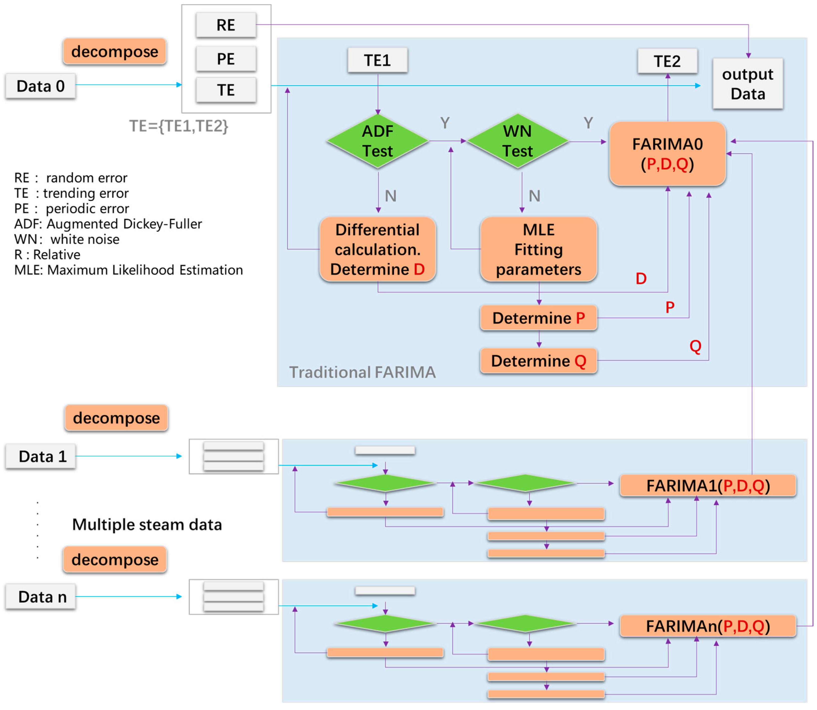
FARIMA is a prediction model used to handle long-term time-series data. It combines autoregressive moving average (ARMA) models with fractional differencing to acquire long-term dependencies in data [28,29]. Traditional FARIMA algorithms can only predict single types of continuous data, and their accuracy decreases when an RE plays a role in the data. As the employed ephemeris data are of different types and are discrete, the MS-FARIMA algorithm is expected to improve the error. The MS-FARIMA algorithm design is shown in Figure 5.

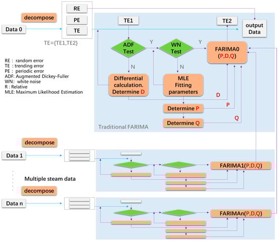
Figure 5. MS-FARIMA framework.

Firstly, we assume multiple discrete data sequences $\{a\left[0\right], a\left[1\right],\dots ,a[\mathrm{i}-1],a\left[i\right],\dots ,a\left[n\right]\}$ and calculate K sets of the error values via K sets of predicted data sequences and K sets of accurate data sequences. A fusion operator $A(·)$ is defined to establish and eliminate the common RE among the multiple data sets.

Next, after eliminating the RE, a $\mathit{FARIMA}\left(p,d,q\right)$ model is constructed for the multiple sets of discrete data, which can be expressed as

$$\mathsf{\Phi }(B){\Delta }^d{X}_t=\mathsf{\Theta }(B)a_t$$

(24)

where $B$ is a defined delay operator, $B{X}_t=X_{t-1}$, and $a_t$ is an independent, normally distributed white noise sequence. The coefficient polynomial for the differenced autoregressive term is $\mathit{\Phi }\left(B\right)=1-{\varphi }_{1}B-\cdots -{\varphi }_p{B}^p$, where p is the autoregressive order. The coefficient polynomial for the moving average term is $\mathsf{\Theta }\left(B\right)=1-{\theta }_{1}B-\cdots -{\theta }_q{B}^q$, whereas q is the moving average order.

${\Delta }^d$ is the fractional differencing operator, which is specifically expressed as follows:

$${\Delta }^d={(1-B)}^d={\displaystyle \sum _{k=0}^{\infty }\left(\begin{array}{c}d\\ k\end{array}\right){(-B)}^k}$$

(25)

where

$$\left(\begin{array}{c}d\\ k\end{array}\right)={\displaystyle \frac{\mathsf{\Gamma }(d+1)}{\mathsf{\Gamma }(k+1)\mathsf{\Gamma }(d-k+1)}}$$

(26)

Γ represents the Gamma function, $d$ is the fractional differencing coefficient, and $k$ is the summation index variable. When considering long-term dependence, the value of $d$ lies within $\left(0,0.5\right)$.The larger the value, the more pronounced the long-term dependence of the series.

The specific procedure for the application of the $\mathit{FARIMA}\left(p,d,q\right)$ prediction model to multiple sets of discrete data is shown as follows.

(a)

Determine the differencing order $d$ to achieve stationarity in the data series. For the discrete data series $a\left[i\right]$, set the differencing order $d$ that satisfies ${\Delta }^d=(1-B{)}^d$. Through multiple differencing processes, obtain a stationary data series $a^{\prime }\left[i\right]$;

(b)

Determine the coefficients $p$ for the autoregressive terms and $q$ for the moving average terms. Using the above formulas, employ the Akaike information criterion (AIC) to determine the orders $p$ and $q$. The values of $p$ and $q$ are obtained when the AIC value is minimized;

(c)

Fit the model parameters using maximum likelihood estimation (MLE). This step results in the final $\mathit{FARIMA}\left(p,d,q\right)$ prediction model;

(d)

Predict the values for each data set using the derived prediction model. Apply the model to each group of data to obtain the prediction sequences for the respective discrete data sets.

The MS-FARIMA algorithm leverages the complementarity among multiple data sets to eliminate the impact of RE on the predictions. Consequently, this algorithm offers higher prediction accuracy compared to traditional FARIMA algorithms.

4.2. MS-FARIMA Algorithm for Orbit Extrapolation Based on MSEC

4.2.1. MSEC for Elimination of Ephemeris Errors

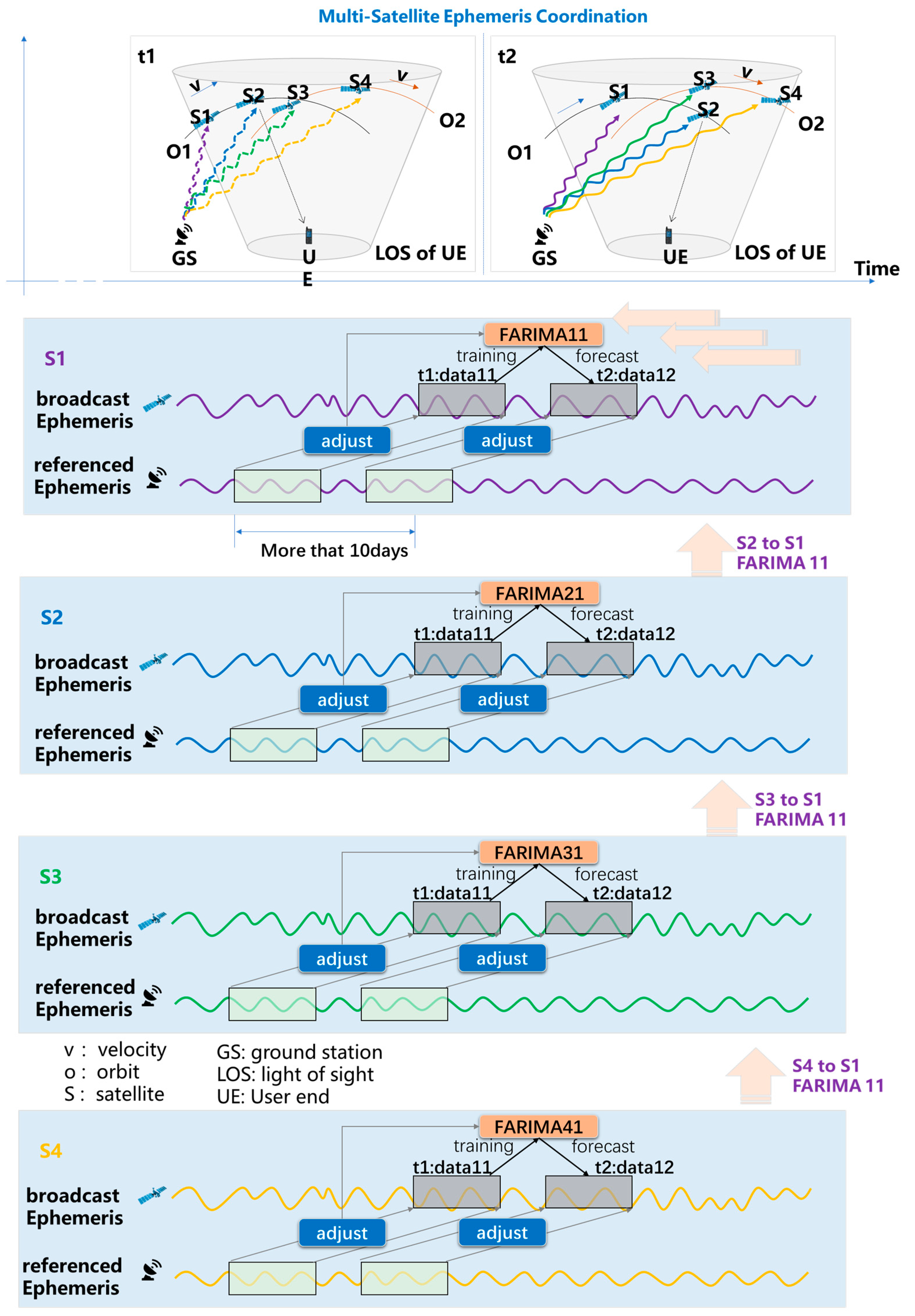
As shown in Figure 6, in the LEO-SIN, the UE has a certain LOS range for satellites based on the strength of the received signals. Within this LOS range, the UE can fully receive the ephemeris information broadcast by the satellites. Satellites in the same constellation have similar orbital altitudes, satellite characteristics, and corresponding orbital characteristics. This is especially true for satellites on the same or adjacent orbits. Therefore, the ephemeris broadcast by these satellites also exhibits a certain degree of similarity. Based on this characteristic, research into the collaborative use of multiple satellites’ ephemeris information can optimize the accuracy of ephemeris estimation.

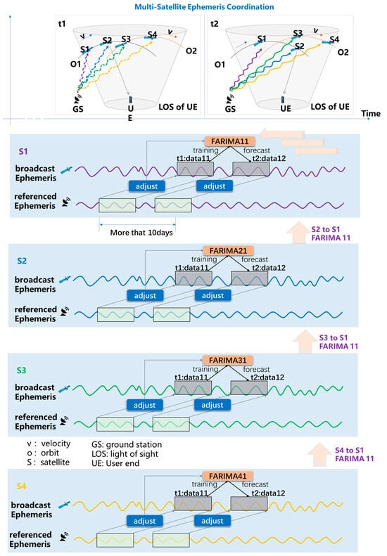
Figure 6. MS-FARIMA algorithm for orbit extrapolation based on MSEC.

The algorithm first uses the ephemeris data from satellites preceding and following on the same orbit and adjacent satellites on different orbits to eliminate the RE through MSEC error elimination. At any given time, the UE simultaneously receives ephemerides from several satellites. This includes satellites on the same orbit as the current satellite, as well as those on different orbits. The UE integrates and corrects these ephemeris data to eliminate the RE.

At time t, we assume that the UE can receive K visible satellites’ ephemeris data ${\mathcal{T}}_{{\mathcal{L}}_{i,t}}$ at the beam position ${\mathcal{L}}_i$. Using the reference time $t_{\mathit{oe}}$ and the SKOEs in the TLE ephemeris data, the SGP4 algorithm is used to extrapolate the three-dimensional coordinate components of the position vector r, as shown in Equation (27). Based on the broadcast ephemeris received from the K different satellites, the spatial position errors for the K different positions can be calculated:

$$\left[\begin{array}{c}\delta x_i(t)\\ \delta y_i(t)\\ \delta z_i(t)\end{array}\right]=\left[\begin{array}{c}{\displaystyle \frac{\partial x(P_t,t_{oe},t)}{\partial n}},\cdots ,{\displaystyle \frac{\partial x(P_t,t_{oe},t)}{\partial \mathsf{\Omega }}}\\ {\displaystyle \frac{\partial y(P_t,t_{oe},t)}{\partial n}},\cdots ,{\displaystyle \frac{\partial y(P_t,t_{oe},t)}{\partial \mathsf{\Omega }}}\\ {\displaystyle \frac{\partial z(P_t,t_{oe},t)}{\partial n}},\cdots ,{\displaystyle \frac{\partial z(P_t,t_{oe},t)}{\partial \mathsf{\Omega }}}\end{array}\right]\left[\begin{array}{c}\delta n\\ \delta i\\ ⋮\\ \delta \mathsf{\Omega }\end{array}\right]$$

(27)

where $\delta n,\delta i,\cdots ,\delta \mathsf{\Omega }$ represent the errors in the SKOEs, $i=1,2,\cdots ,K$ denotes the K satellites where TLE data are received by the UE at time t. $\delta x_i\left(t\right),\delta y_i\left(t\right),\delta z_i\left(t\right)$ represent the three-dimensional coordinate position errors of the i-th ephemeris data. Therefore, the error for the K sets of ephemerides can be expressed as

$$\begin{array}{c}\Delta e^1\begin{array}{c}\underset{=}{def}\\ \end{array}\left(\delta x_1\left(t\right),\delta y_1\left(t\right),\delta z_1\left(t\right)\right)\\ ⋮\\ \Delta e^K\begin{array}{c}\underset{=}{def}\\ \end{array}\left(\delta x_K\left(t\right),\delta y_K\left(t\right),\delta z_K\left(t\right)\right)\end{array}$$

(28)

where $\Delta e^K$ represents the error vector of the ephemeris for the K-th satellite, and $\delta x^K\left(t\right),\delta y^K\left(t\right),\delta z^K\left(t\right)$ represent the error vectors of the K-th satellite’s ephemeris in the X, Y, and Z directions, respectively.

For error assessments in a single direction, error elimination can be performed using the ephemeris currently received from the K − 1 adjacent satellites. The error equations for the ephemeris of the K − 1 satellites in the X direction can be calculated

$$\left\{\begin{array}{c}\delta x_1(t)=f_{n,x}^{\prime }·\delta n+f_{i,x}^{\prime }·\delta i+\cdots +f_{\mathsf{\Omega },x}^{\prime }·\delta \mathsf{\Omega }\\ ⋮\\ \delta x_{i-1}(t)=f_{n,x}^{\prime }·\delta n+f_{i,x}^{\prime }·\delta i+\cdots +f_{\mathsf{\Omega },x}^{\prime }·\delta \mathsf{\Omega }\\ \delta x_{i+1}(t)=f_{n,x}^{\prime }·\delta n+f_{i,x}^{\prime }·\delta i+\cdots +f_{\mathsf{\Omega },x}^{\prime }·\delta \mathsf{\Omega }\\ ⋮\\ \delta x_K(t)=f_{n,x}^{\prime }·\delta n+f_{i,x}^{\prime }·\delta i+\cdots +f_{\mathsf{\Omega },x}^{\prime }·\delta \mathsf{\Omega }\end{array}\right.$$

(29)

where $f_{n,x}^{\prime },f_{i,x}^{\prime },\dots ,f_{\mathsf{\Omega },x}^{\prime }$ represent the sensitivity coefficients of the position error with respect to the SKOE error.

From the above K − 1 equations, deviations in the X direction based on the SKOEs $\delta n,\delta i,\cdots ,\delta \mathsf{\Omega }$ can be determined. By substituting these into the following formula, the deviation in the X direction of the ephemeris $\delta x_i\left(t\right)$ for the current service satellite i received by the UE can be obtained

$$\delta x_i(t)=f_{n,x}^{\prime }·\delta n+f_{i,x}^{\prime }·\delta i+\cdots +f_{\mathsf{\Omega },x}^{\prime }·\delta \mathsf{\Omega }$$

(30)

Similarly, we can obtain the deviations in the Y direction $\delta y_i\left(t\right)$ and the Z direction $\delta z_i\left(t\right)$.

Let $\Delta S\left(t\right)$ be the satellite orbit correction parameter. Based on the above analysis, it can be expressed as

$$\Delta S(t)=(\delta x_i(t),\delta y_i(t),\delta z_i(t))$$

(31)

The corrected ephemeris can be expressed as

$$S_{correction}(t)=S_{boardcast}(t)+\Delta S(t)$$

(32)

where $S_{\mathit{correction}}\left(t\right)$ is the corrected position vector and $S_{\mathit{boardcast}}\left(t\right)$ is the position vector calculated from the TLE ephemeris data.

4.2.2. MS-FARIMA Algorithm for Elimination of Ephemeris Errors

According to the previous analysis, the RE can be eliminated through MSEC. After eliminating the RE, we define the ephemeris error data as $S_{\mathit{orbit}}^{\prime }\left(t\right)$. They can be decomposed into PE $S\left(t\right)$ and TE $R\left(t\right)$:

$$S_{orbit}^{\prime }(t)=R(t)+S(t)$$

(33)

TE $R\left(t\right)$ reflects the ephemeris data errors in different scenarios. However, it can be predicted for certain periods in the future based on the known sequence using the TSF algorithm. This study uses the MS-FARIMA algorithm to predict TE $R\left(t\right)$ for a future period.

We construct a $\mathit{FARIMA}\left(p,d,q\right)$ model for $R\left(t\right)$. The details are as follows.

(a)

Determine the differencing order d to render TE $R\left(t\right)$ stationary. For TE $R\left(t\right)$, set the differencing order d such that ${\Delta }^d={(1-B)}^d$. The stationary TE $R^{\prime }\left(t\right)$ is obtained through multiple differencing processes;

(b)

Determine the coefficients p of the autoregressive terms and the q of the moving average terms. Select the orders p and q using the AIC. The values of p and q are chosen such that the AIC value is minimized;

(c)

Fitting the model parameters using the MLE, eventually we obtain the predictive model $\mathit{FARIMA}\left(p,d,q\right)$;

(d)

Predict TE $R\left(t\right)$ for a future period using the obtained predictive model $\mathit{FARIMA}\left(p,d,q\right)$. We assume that the resulting values are $R^{″}\left(t\right)$, which satisfies the following equation:

$$R^{″}(t+\Delta t)=FARIMA(p,d,q)R(t)$$

(34)

where $\Delta t$ represents the discrete sampling interval of the real ephemeris.

(e)

The final ephemeris’ predicted position $S_{\mathit{orbit}}^{″}\left(t\right)$ is obtained from the predicted component $R^{″}\left(t\right)$ and the PE $S\left(t\right)$, which can be expressed as

$$S_{orbit}^{″}(t)=R^{″}(t)+S(t)$$

(35)

The specific implementation process is shown in Algorithm 1.

Algorithm 1. MS-FARIMA algorithm
Input:	TLE data of K satellites: precise ephemeris ${\mathit{eph}}_{\mathit{precise}}$ for K satellites over the discrete time interval from 1 to $T_d$
Output:	Prediction results
01:	Initialize differencing order d
02:	for satellite $i=1:K$
03:	Read the SKOEs $n_i,i_i,e_i,M_i,{\omega }_i,{\mathsf{\Omega }}_i$ of satellite i from $TL{E}_i$
04:	Input the SKOEs of satellite i into the SGP4 algorithm to obtain the velocity $V_i(v_x,v_y,v_z)$ and position $R_i(r_x,r_y,r_z)$ of satellite i
05:	Calculate the ephemeris error from the SGP4 algorithm as ${\Delta }_i=R_i-{\mathit{eph}}_{\mathit{precise}}\left(i\right)$
06:	End
07:	Substitute the $K$ error values ${\Delta }_i$ into Equations (22) and (23). Use the function $solve$ to solve the equations and obtain the current service satellite error $S_{\mathit{orbit}}^{\prime }\left(t\right)$ after eliminating the RE
08:	Do
09:	Use the function findpeaks to extract the upper and lower extrema of $S_{\mathit{orbit}}^{\prime }\left(t\right)$, yielding the extrema sets $\mathit{ul}\left(t\right)$ and $\mathit{dl}\left(t\right)$, and calculate the mean $\mathit{ml}\left(t\right)$
10:	Calculate $g\left(t\right)=S_{\mathit{orbit}}^{\prime }\left(t\right)-\mathit{ml}\left(t\right)$ to obtain $g\left(t\right)$
11:	While $g_i\left(t\right)$ is not an intrinsic function
12:	Obtain the TE component ${Y\left(t\right)}_{\mathit{trend}}={\sum }_{i=1}^n{g}_i\left(t\right)$
13:	Use the function FFT to perform a fast Fourier transform on $S_{\mathit{orbit}}\left(t\right)$ to obtain the PE component ${Y\left(t\right)}_{\mathit{trend}}$
14:	Do
15:	$d=d+0.1$
16:	Perform d-order differencing on ${Y\left(t\right)}_{\mathit{trend}}$ to obtain ${Y\left(t,i\right)}_{\mathit{trend}}$
17:	While ${Y\left(t,i\right)}_{\mathit{trend}}$ is stationary
18:	Perform autocorrelation on ${Y\left(t,i\right)}_{\mathit{trend}}$ and determine q based on the results
19:	Perform partial autocorrelation on ${Y\left(t,i\right)}_{\mathit{trend}}$ and determine p based on the results
20:	Use the $\mathit{FARIMA}\left(p,d,q\right)$ model to predict the discrete points in the interval from $T_d/2$ to $T_d$ and output the final prediction results

4.3. Theoretical Performance Analysis

At time t, we assume that the UE can obtain the broadcast ephemeris from the currently serving satellite ${\mathit{satellite}}_{\mathit{service}}$ as $\mathit{eph}\_\mathit{broadcast}={\mathit{eph}}_{t,0}$; ${\mathit{eph}}_{t,0}$ represents the ephemeris broadcast by the satellite at time t, and ${\mathit{eph}}_{t,J}$ represents the ephemeris that the UE can receive from other satellites. $J$ is the orbital matrix, which can be expressed as

$$J=\{j_n,j_k\}$$

(36)

where $j_n$ represents n-th satellites before or after the current satellite ${\mathit{satellite}}_{\mathit{service}}$ on the same orbit, $j_k$ represents k-th satellites before or after the current satellite ${\mathit{satellite}}_{\mathit{service}}$ on the adjacent orbit.

Based on the previous analysis, ${\mathit{eph}}_{t,J}$ includes three types of errors: RE $\Delta {\mathit{eph}}_{t,k}\left(\mathit{rand}\right)$, TE $\Delta {\mathit{eph}}_{t,k}\left(\mathit{trend}\right)$, and PE $\Delta {\mathit{eph}}_{t,k}\left(\mathit{period}\right)$. The ephemeris satisfies the following matrix:

$$C_{eph}=\left[\begin{array}{ccc}ep{h}_{t-T_t,k-1}& ep{h}_{t-T_t,k}& ep{h}_{t-T_t,k+1}\\ ep{h}_{t,k-1}& ep{h}_{t,k}& ep{h}_{t,k+1}\\ ep{h}_{t-T_t,k-1}& ep{h}_{t-T_t,k-1}& ep{h}_{t-T_t,k+1}\end{array}\right]$$

(37)

where ${\mathit{eph}}_{t,k}$ is the broadcast ephemeris from the currently serving satellite. Simultaneously, the UE can look up the corresponding broadcast ephemeris ${\mathit{eph}}_{t-T_t,k}$ from the time $t-T_t$. Currently, the broadcast ephemerides of the two satellites before and after the current one on the same orbit are ${\mathit{eph}}_{t,k-1}$ and ${\mathit{eph}}_{t,k+1}$.

We assume the MSEC operator $A(·)$; this operator will eliminate the RE $∆{\mathit{eph}}_{t,k}\left(\mathit{rand}\right)$ coexisting among multiple satellites, which can be expressed as

$$A(C_{eph})=\left[\begin{array}{ccc}ep{h}_{t-T_t,k-1}^{\prime }& ep{h}_{t-T_t,k}^{\prime }& ep{h}_{t-T_t,k+1}^{\prime }\\ ep{h}_{t,k-1}^{\prime }& ep{h}_{t,k}^{\prime }& ep{h}_{t,k+1}^{\prime }\\ ep{h}_{t-T_t,k-1}^{\prime }& ep{h}_{t-T_t,k-1}^{\prime }& ep{h}_{t-T_t,k+1}^{\prime }\end{array}\right]$$

(38)

where ${\mathit{eph}}_{t,k}^{\prime }$ represents the broadcast ephemeris after the elimination of the RE $\Delta {\mathit{eph}}_{t,k}\left(\mathit{rand}\right)$ using MSEC:

$$ep{h}_{t,k}^{\prime }=\Delta ep{h}_{t,k}(trend)+\Delta ep{h}_{t,k}(period)$$

(39)

For PE $\Delta {\mathit{eph}}_{t,k}\left(\mathit{period}\right)$, due to its periodic characteristics, spectral analysis can be used to extract the PE:

$$SPE(ep{h}_{t,k}^{\prime })=\Delta ep{h}_{t,k}(period)$$

(40)

Then, TE $\Delta {\mathit{eph}}_{t,k}\left(\mathit{trend}\right)$ can be expressed as

$$\Delta ep{h}_{t,k}(trend)=ep{h}_{t,k}^{\prime }-\Delta ep{h}_{t,k}(period)$$

(41)

For TE $∆{\mathit{eph}}_{t,k}\left(\mathit{trend}\right)$, MS-FARIMA is used to eliminate the TE:

$$Tim{e}_{predict}(\Delta ep{h}_{t,k}(trend))=\Delta ep{h}_{t,k}^{\prime }(period)$$

(42)

where $\Delta {\mathit{eph}}_{t,k}^{\prime }\left(\mathit{trend}\right)$ is the new TE after eliminating TE $\Delta {\mathit{eph}}_{t,k}\left(\mathit{trend}\right)$ using MS-FARIMA.

The originally broadcast ephemeris from the initial analysis can be expressed as

$$\begin{array}{l}ep{h}_{broadcast}(t,k)=ep{h}_0+\Delta ep{h}_{t,k}\\ =ep{h}_0+\Delta ep{h}_{t,k}(rand)+\Delta ep{h}_{t,k}(period)+\Delta ep{h}_{t,k}(trend)\end{array}$$

(43)

After using MSEC and MS-FARIMA, the broadcast ephemeris can be expressed as

$$ep{h}_{broadcast}^{\prime }(t,k)=ep{h}_0+\Delta ep{h}_{t,k}^{\prime }(trend)$$

(44)

From Equation (44), the ephemeris error is smaller than the original ephemeris error. Therefore, MSEC and the MS-FARIMA model can effectively eliminate ephemeris errors.

5. Simulation and Mathematical Analysis

5.1. Simulation Configuration

In our simulation, the test ephemeris data exploit the sample ephemeris data of the STARLINK-2569 satellite. The parameter configuration of this satellite is shown in Table 2. We prepare two groups of data: one group is the referenced ephemeris data, which are accurate (downloaded from www.space-track.org), and the other group is the test ephemeris data, which are the broadcast TLE ephemeris data (downloaded from celestrak.org).

Table 2. Satellite parameters.

Parameter	IRIDIUM-143	STARLINK-2569
Mean orbital altitude (km)	789.86	554.4
Orbital inclination (degrees)	86.4	53.056
Period (minutes)	102.86	95.593
Eccentricity	0.00011	0.00015

The parameter configuration of the second line of the TLE data is shown in Table 3.

Table 3. The second line of TLE data.

Parameter	Value
Gravitational constant $G/(N·{\mathrm{m}}^2/{\mathrm{kg}}^2)$	$6.67\times {10}^{-11}$
Earth’s mass $\mathrm{M}/\left(\mathrm{kg}\right)$	$5.965\times {10}^{24}$
Second-order Earth gravitational harmonic $J_2$	$1.0826158\times {10}^{-3}$
Second-order Earth gravitational harmonic $J_3$	$-2.53881\times {10}^{-6}$
Second-order Earth gravitational harmonic $J_4$	$-1.65597\times {10}^{-6}$
Earth’s equatorial radius $\mathrm{KMPER}/\left(\mathrm{km}\right)$	$6378.135$
Iterative tolerance $\Delta (E+\omega )$	$1\times {10}^{-6}$
Earth’s flattening $\in$	$3.3528\times {10}^{-3}$

5.2. Performance of Orbit Extrapolation

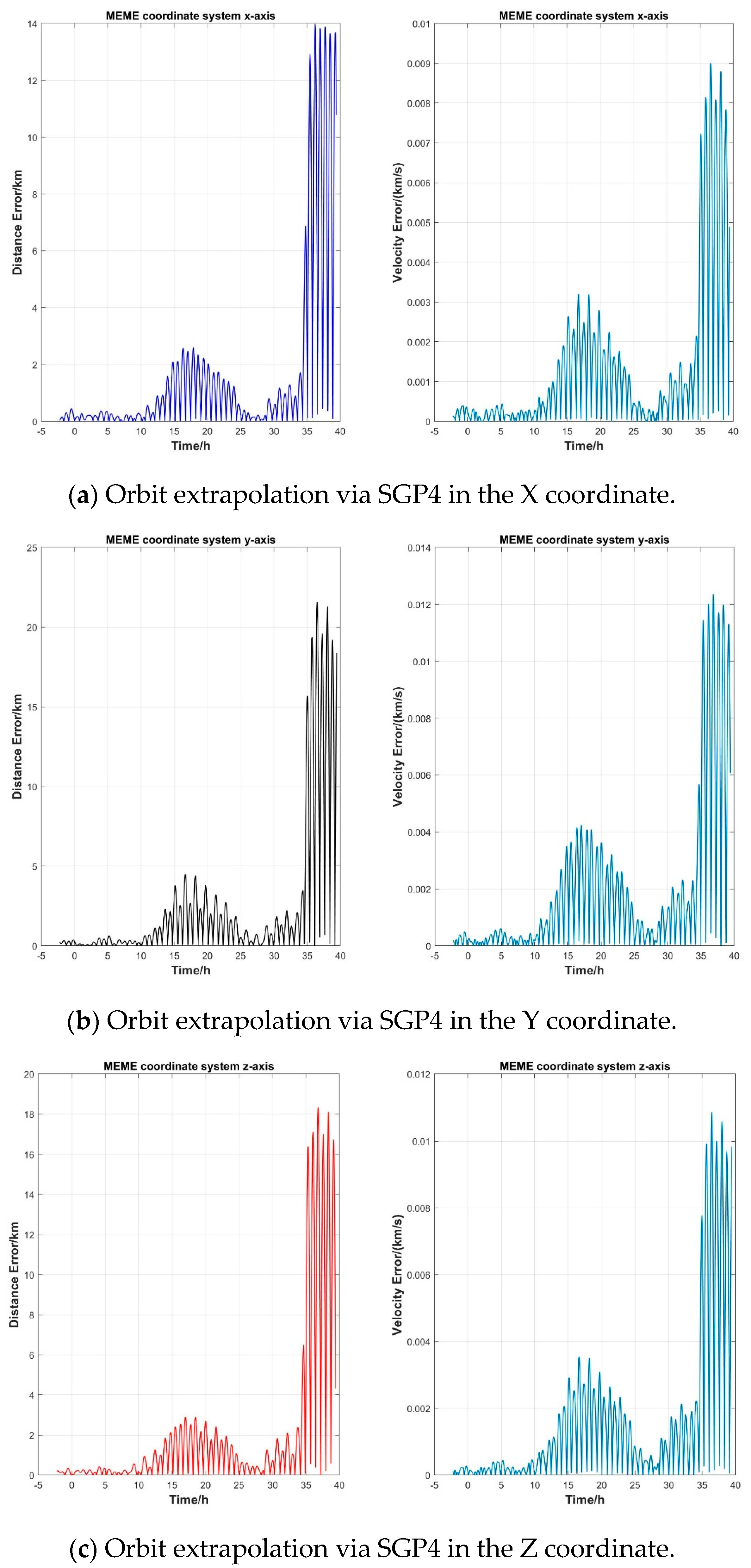
Figure 7 shows the distance error and velocity error of orbit extrapolation from $t=1$ to $t=30$ h when using the SGP4 algorithm in the X, Y, and Z coordinates. Here, due to the SGP4 algorithm employing the TEME coordinate system and the accurate ephemeris adopting the mean equator and mean equinox (MEME) coordinate system, the values from the TEME coordinate system are first transformed to the MEME coordinate system.

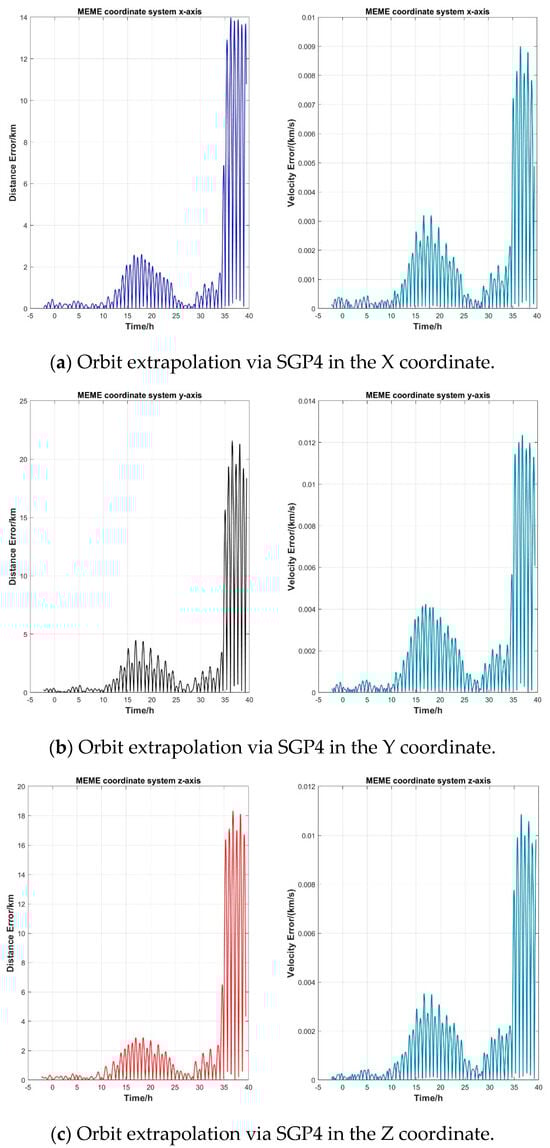
Figure 7. SGP4 ephemeris prediction errors (a) in the X coordinate, (b) Y coordinate, and (c) Z coordinate.

As Figure 7 shows, the orbit extrapolation errors in the X, Y, and Z coordinates are within 0.5 km for extrapolations after less than 10 h. However, the orbit extrapolation errors start to increase after 10 h. Subsequently, the errors begin to fluctuate but generally show an increasing trend. When the satellite is in orbit, it is affected by various perturbative forces, the magnitudes and directions of which are complex and constantly changing. In most cases, the ephemeris extrapolation error tends to increase. However, in some specific situations, the error may fluctuate within a certain range. Nonetheless, it still shows an increasing trend overall. These fluctuations may be caused by the characteristics of the extrapolation algorithm itself, the periodic variations in the satellite’s orbit, or other external factors. The position error of the orbit extrapolation in the X coordinate is smaller compared to that in the Y and Z directions. Both the velocity TE and position TE of orbit extrapolation are similar in the X, Y, and Z coordinates. The position errors are larger than the velocity errors. Here, we noted that the observed start time is −2.22 h because the TLE reference time is within the accurate ephemeris’ given period.

The further statistical results of the SGP4 algorithm are shown in Table 4 and Table 5. As these tables show, the velocity errors of orbit extrapolation are smaller, with RMS values of around 0.001, whereas the position errors are larger. The extrapolation errors in the X, Y, and Z coordinates increase significantly after 10 h. Therefore, the orbit extrapolation algorithm based on the MS-FARIMA model will exploit ephemeris data in the X, Y, and Z coordinates from the first 10 h as input training data to then extrapolate the satellite orbit beyond 10 h. Since the ephemeris data in the X, Y, and Z coordinates are similar, we only present the performance of the extrapolation of the X coordinate of the ephemeris data.

Table 4. The statistics of the STARLINK-2569 distance error.

Prediction (30 h)	ΔX/km	ΔY/km	ΔZ/km
Maximum	2.47	4.48	2.53
RMS	0.88	1.32	1.01

Table 5. The statistics of the STARLINK-2569 velocity error.

Prediction (30 h)	$\mathbf{\Delta }{\mathit{V}}_{\mathit{x}}(\mathbf{k}\mathbf{m}/\mathbf{s})$	$\mathbf{\Delta }{\mathit{V}}_{\mathit{y}}(\mathbf{k}\mathbf{m}/\mathbf{s})$	$\mathbf{\Delta }{\mathit{V}}_{\mathit{z}}(\mathbf{k}\mathbf{m}/\mathbf{s})$
Maximum	2.47	4.48	2.53
RMS	0.0010	0.0015	0.0012

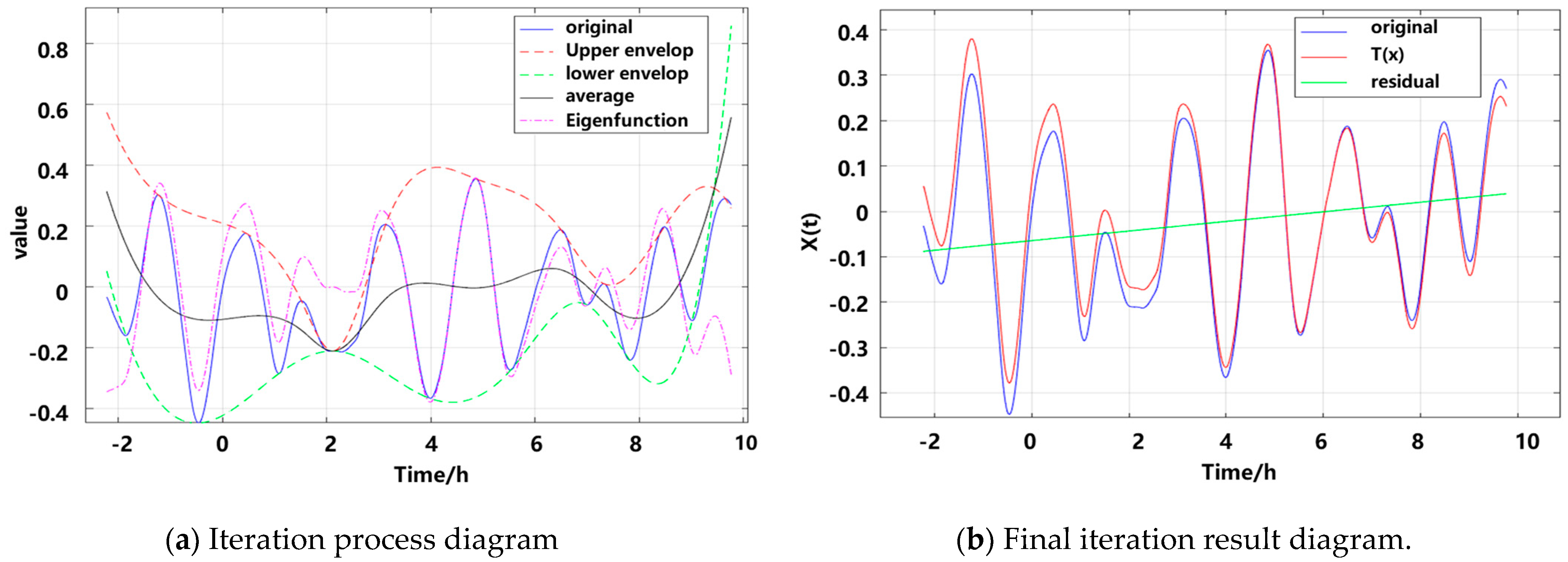
Figure 8 shows the performance of TE extraction and extrapolation. As Figure 8 shows, based on the original data $S_{\mathit{orbit}}^{\prime }\left(t\right)$, the intrinsic function $G_i\left(t\right)$ is obtained through multiple iterations, as depicted in Figure 7. Finally, the TE is derived according to $S_{\mathit{orbit}}^{\prime }\left(t\right)={\sum }_{i=1}^n{G}_i\left(t\right)+{\mathit{r}}_{\mathit{n}+1}\left(t\right)$. The final TE $R\left(t\right)$ is specifically shown in Figure 8b.

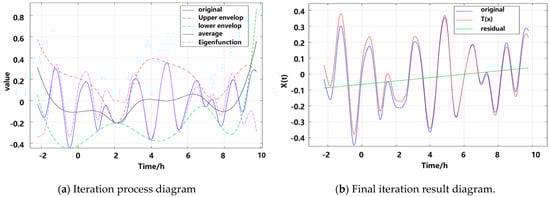
Figure 8. TE extraction and extrapolation performance: (a) iteration process, (b) final iteration result.

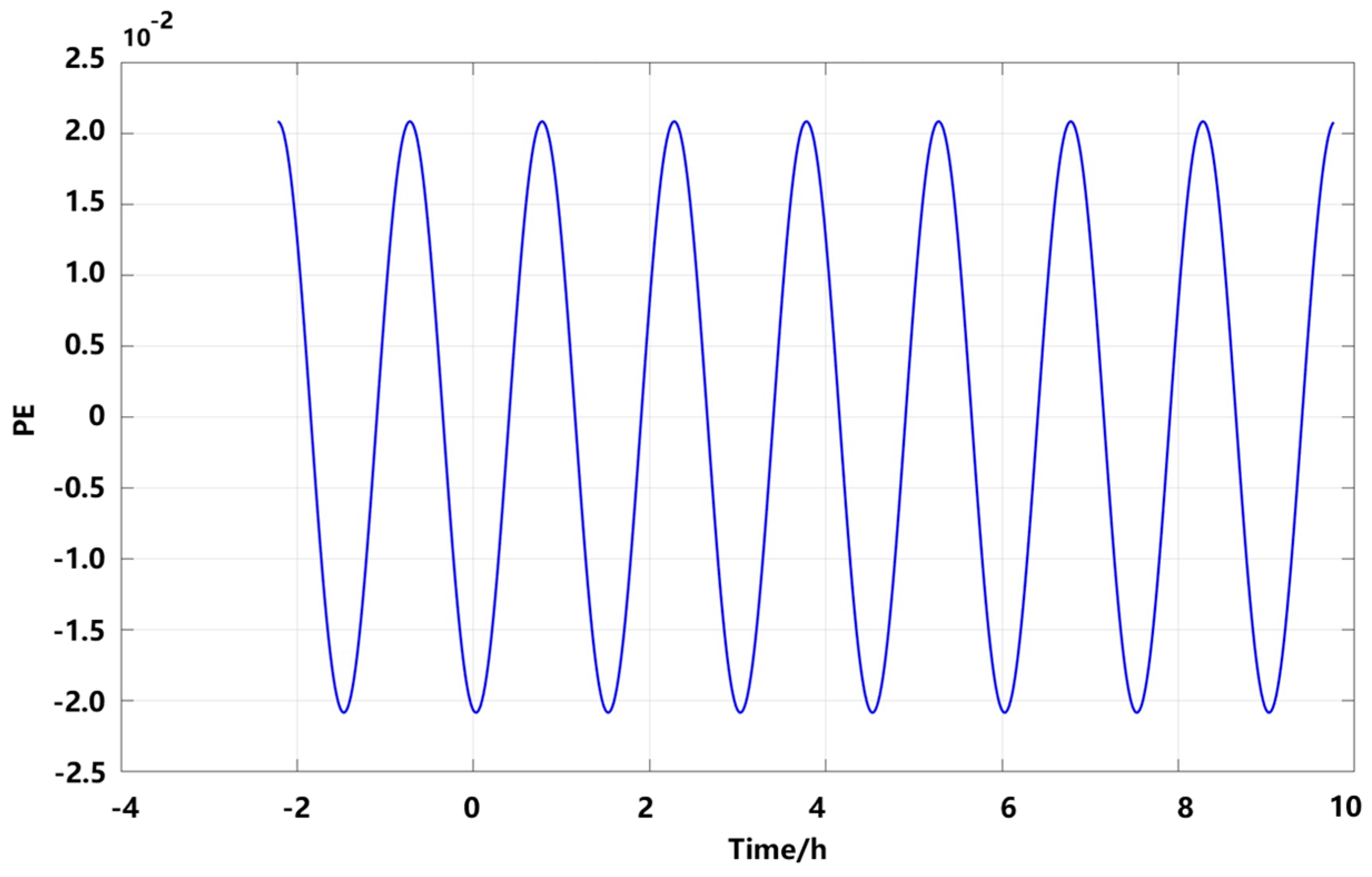
Figure 9 shows the values of the PE obtained through the FFT and spectral analysis. It can be observed that PE $S\left(t\right)$ has a period of 1.517 h and an amplitude of 0.02. This indicates that while a PE exists in $S_{\mathit{orbit}}^{\prime }\left(t\right)$, its overall impact on the values is minimal.

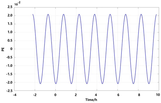
Figure 9. PE extraction and extrapolation performance.

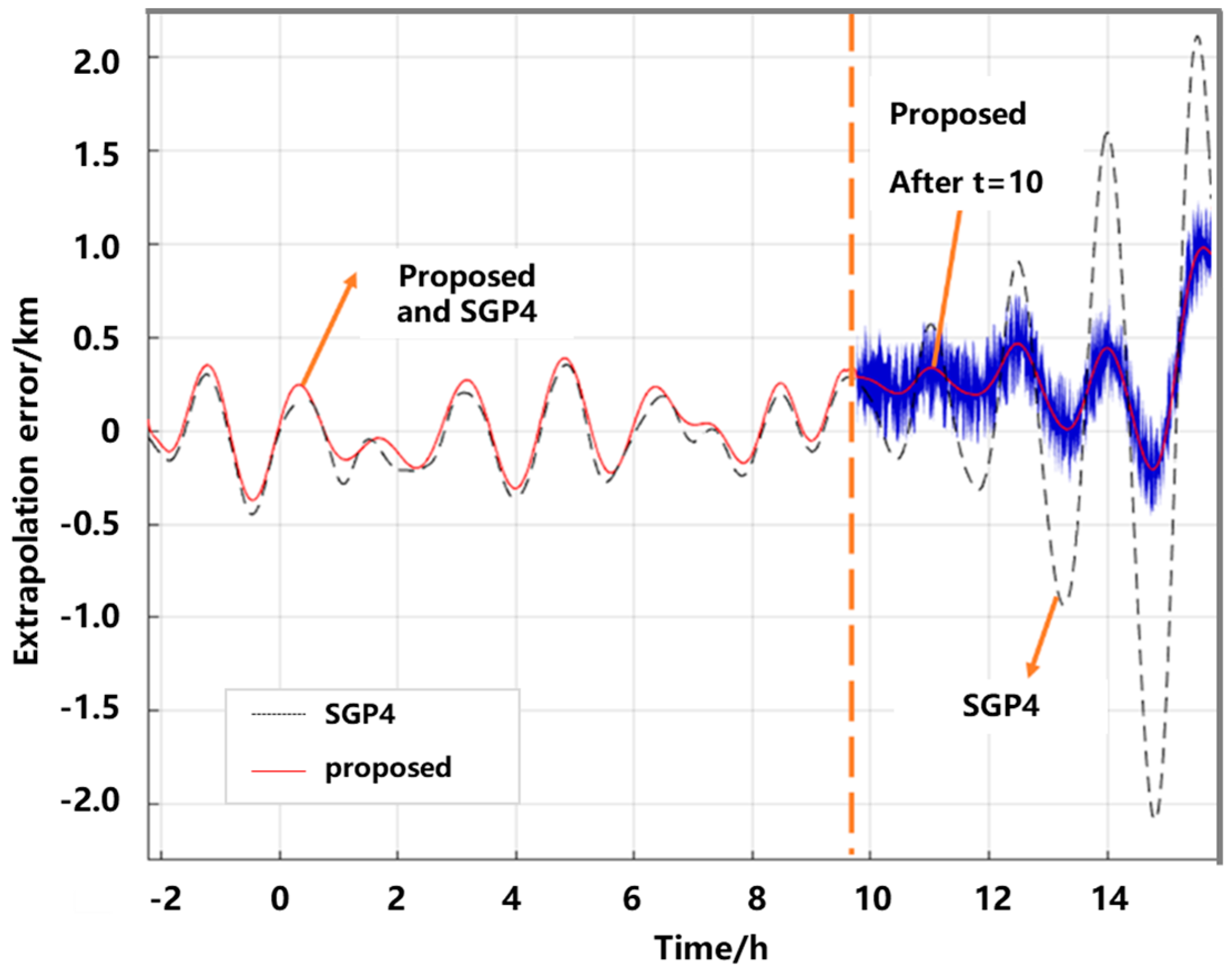
Figure 10 shows the extrapolation results when using the MS-FARIMA model. As Figure 10 shows, before $t=10$ h, the extrapolation error exhibited by the proposed MS-FARIMA is close to that of the original SGP4. After $t=10$ h, it is evident that the optimized extrapolation error for the proposed MS-FARIMA decreases by 33.5% compared to the original SGP4.

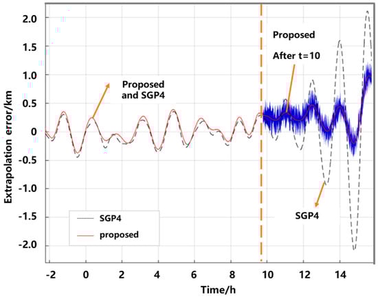
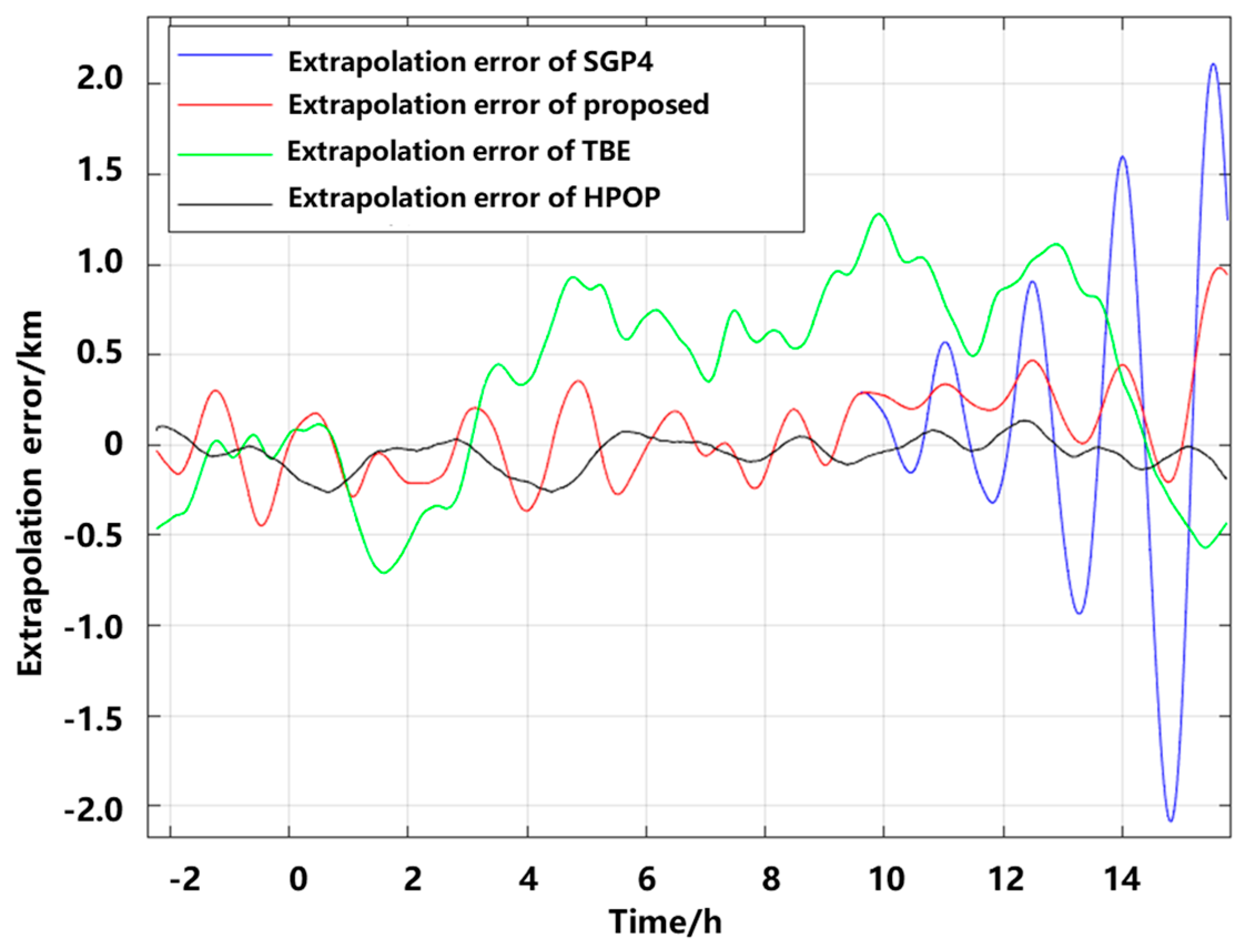
Figure 10. Performance comparison of proposed MS-FARIMA and other existing algorithms.

Figure 10 shows the performance comparison between the proposed algorithm and existing extrapolation algorithms, which are exemplified by the two-body extrapolation (TBE) algorithm, SGP4 algorithm, and the high-precision orbit propagator (HPOP) algorithm. As Figure 11 shows, the extrapolation error of the proposed algorithm is generally within 0.5 km after 15 h. In comparison, the extrapolation error of the SGP4 algorithm is generally beyond 0.5 km after 10 h. In the observed time, the extrapolation error of the two-body extrapolation algorithm is higher than that of the SGP4 algorithm and the proposed algorithm, and is also generally greater than 0.5 km. Additionally, the extrapolation error of HPOP generally remains within 0.3 km over 15 h. However, the HPOP algorithm needs to acquire more ephemeris data through broadcasting. From the experimental results, the prediction errors of all four algorithms exhibit certain fluctuations, but they show an increasing trend overall. This is consistent with the theoretical results.

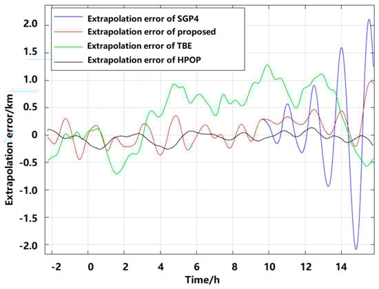
Figure 11. Comparison of ephemeris optimization algorithm errors.

Table 6 shows the mean absolute errors (MAEs) of the four ephemeris optimization algorithm errors. Compared to the traditional SGP4 algorithm, the proposed algorithm’s error shows a significant decrease, second only to the HPOP algorithm. In addition, the proposed algorithm has lower complexity.

Table 6. The MAEs of the ephemeris optimization algorithm errors.

Extrapolation Error	Proposed	SGP4	TBE	HPOP
MAE (km)	0.19	0.3357	0.5589	0.07467
Complexity	Simple	Simple	Simple	Complex

5.3. Optimization of Communication Performance (The Case of DFO Compensation)

Figure 12 shows the simulated DFO examination scenario for the LEO-SIN. This figure shows the trajectory of the satellite over 10 min and the three positions of the UE. Based on the different positions of the UE, the position and velocity can be calculated and the DFO can also be calculated.

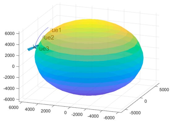
Figure 12. The DFO scenario of the LEO-SIN.

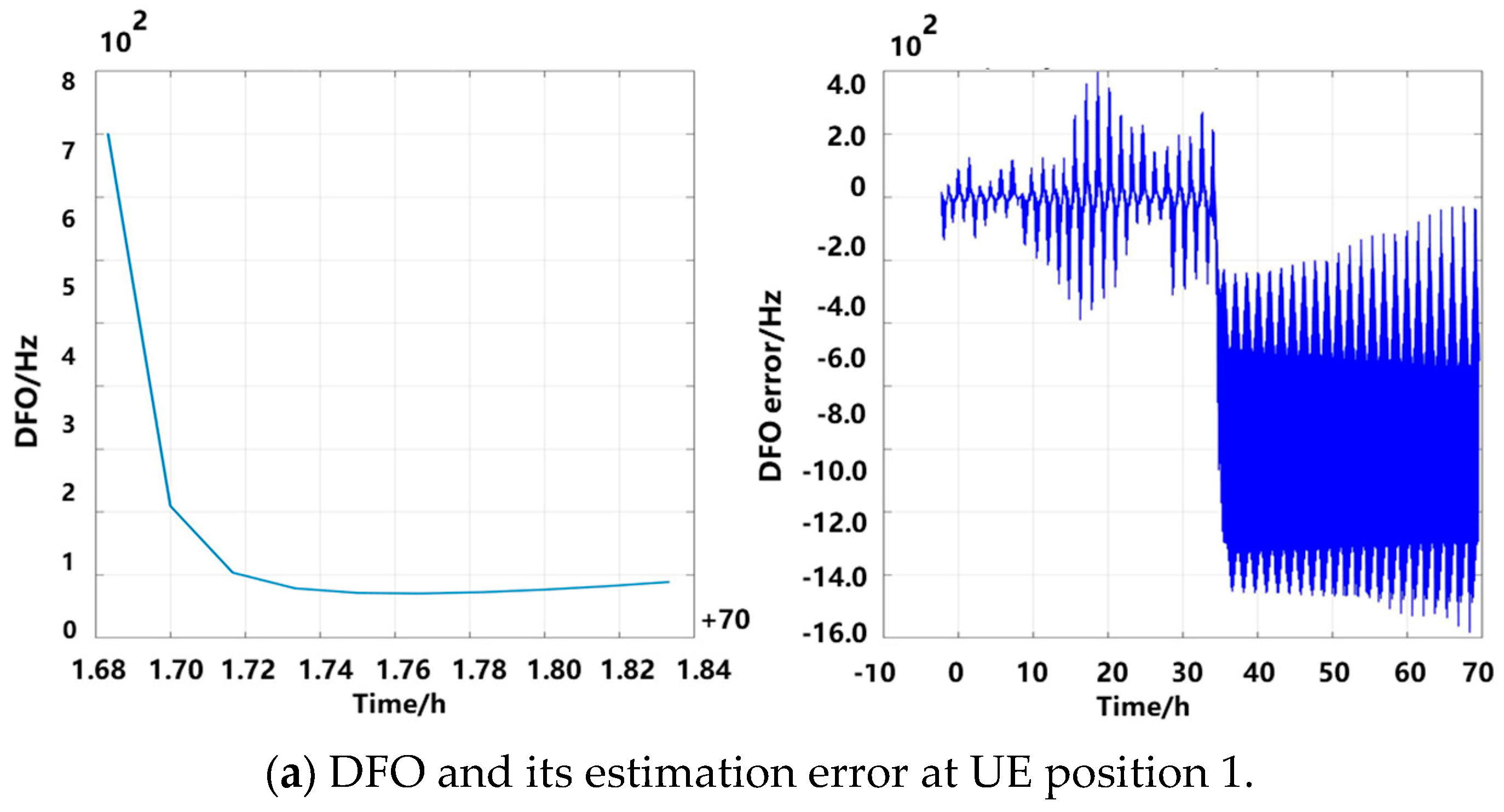
Figure 13 shows the DFO estimation performance of the proposed method. As Figure 13c show, within 35 h the DFO error estimate remains within 400 Hz. The subcarrier spacing used in this simulation is 15 kHz. To meet the requirements, the DFO error should be less than 4% of this spacing, which is 600 Hz. Therefore, using the optimized ephemeris for DFO calculations allows for predictions up to 35 h.

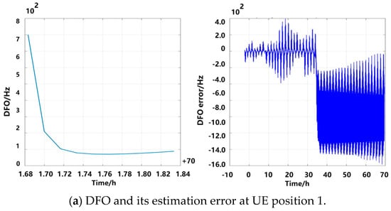
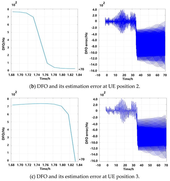
Figure 13. DFO estimation errors based on the proposed method: (a) UE position 1, (b) UE position 2, and (c) UE position 3.

6. Conclusions

This work proposed an LEO-SIN orbit extrapolation method based on MSEC and MS-FARIMA, focusing on solving the problems of low accuracy and low timelessness in existing ephemeris prediction algorithms.

This method decomposed the extrapolation error based on the satellite ephemeris into three categories: RE, TE, and PE. The orbit extrapolation scheme that combines MSEC and MS-FARIMA achieved the elimination of the RE and TE.

This method reduced the ephemeris extrapolation error by 33.5% compared to existing methods, which also contributes to the enhanced performance of DFO estimation in MPDTSC. Future work could incorporate artificial intelligence techniques such as deep learning to further improve the adaptability and accuracy of the orbit extrapolation model.

This work proposed an LEO-SIN orbit extrapolation method based on MSEC and MS-FARIMA. The conclusions are as follows:

• We are the first to propose separating the broadcast ephemeris extrapolation errors into three types: RE, TE, and PE. We focused on improving the extrapolation accuracy by diminishing and compensating for the RE and TE. We also derived the lower bound of the orbit extrapolation error based on single-satellite ephemeris information;
• This work first proposed a novel and accurate ephemeris extrapolation framework that involves the ephemerides of multi-satellite and multi-stream data TSFs;
• An MSEC orbit extrapolation error elimination algorithm that analyzes the spatial and temporal associations between corresponding and different satellites at different times was designed. This algorithm utilized multiple sets of ephemeris information from MSEC to diminish the RE. The focus was primarily on improving the extrapolation accuracy by addressing the RE and TE;
• This work is the first to design an MS-FARIMA algorithm, which supports data from the same attribute information at different times for different objects. The reasons for the improved accuracy of the ephemeris extrapolation error based on MSEC and multi-stream information were also explored;
• The orbit extrapolation scheme that combined MSEC and MS-FARIMA achieved higher accuracy than the single-satellite, single-stream scheme;
• This work proposed a DFO estimation and compensation algorithm for the LEO-SIN based on the employment of the above-optimized ephemeris. It theoretically derives the impacts of different ephemeris errors on DFO estimation, enhancing the DFO estimation accuracy.

References

- Wang, C.X.; You, X.H.; Gao, X.Q.; Zhu, X.M.; Li, Z.X.; Zhang, C.; Hanzo, L. On the Road to 6G: Visions, Requirements, Key Technologies, and Testbeds. IEEE Commun. Surv. Tutor. 2023, 25, 905–974. [Google Scholar] [CrossRef]
- Zidic, D.; Mastelic, T.; Kosovic, I.N.; Cagalj, M.; Lorincz, J. Analyses of ping-pong handovers in real 4G telecommunication networks. Comput. Netw. 2023, 227, 12. [Google Scholar] [CrossRef]
- Premsankar, G.; Piao, G.Y.; Nicholson, P.K.; Di Francesco, M.; Lugones, D. Data-Driven Energy Conservation in Cellular Networks: A Systems Approach. IEEE Trans. Netw. Serv. Manag. 2021, 18, 3567–3582. [Google Scholar] [CrossRef]
- Chen, S.Z.; Sun, S.H.; Miao, D.S.; Shi, T.; Cui, Y.P. The Trends, Challenges, and Key Technologies of Beam-Space Multiplexing in the Integrated Terristrial-Satellite Communication for B5G and 6G. IEEE Wirel. Commun. 2023, 30, 77–86. [Google Scholar] [CrossRef]
- Peng, D.Y.; He, D.X.; Li, Y.; Wang, Z.C. Integrating Terrestrial and Satellite Multibeam Systems Toward 6G: Techniques and Challenges for Interference Mitigation. IEEE Wirel. Commun. 2022, 29, 24–31. [Google Scholar] [CrossRef]
- Guo, F.; Yang, Y.; Ma, F.J.; Zhu, Y.F.; Liu, H.; Zhang, X.H. Instantaneous velocity determination and positioning using Doppler shift from a LEO constellation. Satell. Navig. 2023, 4, 9. [Google Scholar] [CrossRef]
- Wang, D.Y.; Qin, H.L.; Huang, Z.G. Doppler Positioning of LEO Satellites Based on Orbit Error Compensation and Weighting. IEEE Trans. Instrum. Meas. 2023, 72, 11. [Google Scholar] [CrossRef]
- Khairallah, N.; Kassas, Z.M. Ephemeris Tracking and Error Propagation Analysis of LEO Satellites with Application to Opportunistic Navigation. IEEE Trans. Aerosp. Electron. Syst. 2024, 60, 1242–1259. [Google Scholar] [CrossRef]
- Yang, R.H.; Song, Z.G.; Xi, X.L. Self-assisted first-fix method for GPS receiver with autonomous short-term ephemeris prediction. IET Radar Sonar Navig. 2019, 13, 1974–1980. [Google Scholar] [CrossRef]
- Lu, W.Q.; Wang, H.G.; Wu, G.Q.; Huang, Y. Orbit Determination for All-Electric GEO Satellites Based on Space-Borne GNSS Measurements. Remote Sens. 2022, 14, 2627. [Google Scholar] [CrossRef]
- Carlin, L.; Hauschild, A.; Montenbruck, O. Precise point positioning with GPS and Galileo broadcast ephemerides. Gps Solut. 2021, 25, 77. [Google Scholar] [CrossRef]
- Ko, H.; Kyung, Y. Resource- and Neighbor-Aware Observation Transmission Scheme in Satellite Networks. Sensors 2023, 23, 4889. [Google Scholar] [CrossRef] [PubMed]
- Kong, Q.L.; Gao, F.; Guo, J.Y.; Han, L.T.; Zhang, L.G.; Shen, Y. Analysis of Precise Orbit Predictions for a HY-2A Satellite with Three Atmospheric Density Models Based on Dynamic Method. Remote Sens. 2019, 11, 40. [Google Scholar] [CrossRef]
- Gaur, D.; Prasad, M.S. One-Second GPS Orbits: A Comparison Between Numerical Integration and Interpolation. In Proceedings of the 2019 6th International Conference on Signal Processing and Integrated Networks (SPIN), Noida, India, 7–8 March 2019; pp. 973–977. [Google Scholar] [CrossRef]
- Gou, J.; Roesch, C.; Shehaj, E.; Chen, K.; Shahvandi, M.K.; Soja, B.; Rothacher, M. Modeling the Differences between Ultra-Rapid and Final Orbit Products of GPS Satellites Using Machine-Learning Approaches. Remote Sens. 2023, 15, 5585. [Google Scholar] [CrossRef]
- Matsumura, T.; Higashino, T.; Nakagawa, Y.; Okada, M. Machine learning approach for predicting precise ZTD produced by GNSS broadcast ephemeris. In Proceedings of the 2022 IEEE 11th Global Conference on Consumer Electronics (GCCE), Osaka, Japan, 18–21 October 2022; pp. 66–67. [Google Scholar] [CrossRef]
- Thammawichai, M.; Luangwilai, T. Data-driven satellite orbit prediction using two-line elements. Astron. Comput. 2024, 46, 100782. [Google Scholar] [CrossRef]
- Ge, H.; Meng, G.; Li, B. Zero-Reconvergence PPP for Real-Time Low-Earth Satellite Orbit Determination in Case of Data Interruption. IEEE J. Sel. Top. Appl. Earth Obs. Remote Sens. 2024, 17, 4705–4715. [Google Scholar] [CrossRef]
- Wang, K.; Liu, J.W.; Su, H.; El-Mowafy, A.; Yang, X.H. Real-Time LEO Satellite Orbits Based on Batch Least-Squares Orbit Determination with Short-Term Orbit Prediction. Remote Sens. 2023, 15, 133. [Google Scholar] [CrossRef]
- Zhuang, Y.; Wang, L.; Zhou, H. Real-time Kinematic Orbit Determination of GRACE D Satellite Using GPS Broadcast Ephemeris. In Proceedings of the 2023 IEEE International Conference on Unmanned Systems (ICUS), Hefei, China, 13–15 October 2023; pp. 937–942. [Google Scholar] [CrossRef]
- Mukundan, A.; Wang, H.C. Simplified Approach to Detect Satellite Maneuvers Using TLE Data and Simplified Perturbation Model Utilizing Orbital Element Variation. Appl. Sci. 2021, 11, 10181. [Google Scholar] [CrossRef]
- Asraf, A.; Surayuda, R.H.; Ribah, A.Z.; Kamirul; Mukhayadi, M. Determination of Mean Orbital Elements Using GPS Data for LAPAN Satellite Daily Operation. In Proceedings of the 2021 IEEE International Conference on Aerospace Electronics and Remote Sensing Technology (ICARES), Bali, Indonesia, 3–4 November 2021; pp. 1–6. [Google Scholar] [CrossRef]
- Boquet, G.; Martinez, B.; Adelantado, F.; Pages, J.; Ruiz-de-Azua, J.A.; Vilajosana, X. Low-Power Satellite Access Time Estimation for Internet of Things Services Over Nonterrestrial Networks. IEEE Internet Things J. 2024, 11, 3206–3216. [Google Scholar] [CrossRef]
- Campiti, G.; Brunetti, G.; Braun, V.; Di Sciascio, E.; Ciminelli, C. Orbital kinematics of conjuncting objects in Low-Earth Orbit and opportunities for autonomous observations. Acta Astronaut. 2023, 208, 355–366. [Google Scholar] [CrossRef]
- Chen, J.Y.; Lin, C.S. Research on Enhanced Orbit Prediction Techniques Utilizing Multiple Sets of Two-Line Element. Aerospace 2023, 10, 532. [Google Scholar] [CrossRef]
- Du, Y.S.; Qin, H.L.; Zhao, C. LEO Satellites/INS Integrated Positioning Framework Considering Orbit Errors Based on FKF. IEEE Trans. Instrum. Meas. 2024, 73, 14. [Google Scholar] [CrossRef]
- Bian, H.X.; Liu, R.K. Reliable and Energy-Efficient LEO Satellite Communication with IR-HARQ via Power Allocation. Sensors 2022, 22, 3035. [Google Scholar] [CrossRef] [PubMed]
- Yang, J.; Sheng, H.; Wan, H.; Yu, F. FARIMA Model Based on Particle Swarm-genetic Hybrid Algorithm Optimization and Application. In Proceedings of the 2021 3rd International Academic Exchange Conference on Science and Technology Innovation (IAECST), Guangzhou, China, 10–12 December 2021; pp. 188–192. [Google Scholar] [CrossRef]
- Christian, G.A.; Wijaya, I.P.; Sari, R.F. Network Traffic Prediction of Mobile Backhaul Capacity Using Time Series Forecasting. In Proceedings of the 2021 International Seminar on Intelligent Technology and Its Applications (ISITIA), Surabaya, Indonesia, 21–22 July 2021; pp. 58–62. [Google Scholar] [CrossRef]
Disclaimer/Publisher’s Note: The statements, opinions and data contained in all publications are solely those of the individual author(s) and contributor(s) and not of MDPI and/or the editor(s). MDPI and/or the editor(s) disclaim responsibility for any injury to people or property resulting from any ideas, methods, instructions or products referred to in the content. |
© 2024 by the authors. Licensee MDPI, Basel, Switzerland. This article is an open access article distributed under the terms and conditions of the Creative Commons Attribution (CC BY) license (https://creativecommons.org/licenses/by/4.0/).