Abstract
Unmanned aerial vehicles (UAVs) are increasingly significant in modern warfare due to their versatility and capacity to perform high-risk missions without risking human lives. Beyond surveillance and reconnaissance, UAVs with jet propulsion and engagement capabilities are set to play roles similar to conventional jets. In various scenarios, military aircraft, drones, and UAVs face multiple threats while ground radar systems continuously monitor their positions. The interaction between these aerial platforms and radars causes temporal fluctuations in scattered echo power due to changes in aspect angle, impacting radar tracking accuracy. This study utilizes the potential radar cross-section (RCS) dynamics of an aircraft throughout its flight, using ground radar as a reference. Key factors influencing RCS include time, frequency, polarization, incident angle, physical geometry, and surface material, with a focus on the complex scattering geometry of the aircraft. The research evaluates the monostatic RCS case and examines the impact of attitude variations on RCS scintillation. Here, we present dynamic RCS modeling by examining the influence of flight dynamics on the RCS fluctuations of a UAV-sized aircraft. Dynamic RCS modeling is essential in creating a robust framework for operational analysis and developing effective countermeasure strategies, such as advanced active decoys. Especially in the cognitive radar concept, aircraft will desperately need more dynamic and adaptive active decoys. A methodology for calculating target aspect angles is proposed, using the aircraft’s attitude and spherical position relative to the radar system. A realistic 6DoF (6 degrees of freedom) flight data time series generated by a commercial flight simulator is used to derive aircraft-to-radar aspect angles. By estimating aspect angles for a simulated complex flight trajectory, RCS scintillation throughout the flight is characterized. The study highlights the importance of maneuver parameters such as roll and pitch on the RCS measured at the radar by comparing datasets with and without these parameters. Significant differences were found, with a 32.44% difference in RCS data between full maneuver and no roll and pitch changes. Finally, proposed future research directions and insights are discussed.
1. Introduction
UAV platforms have received increasing attention from both researchers and industries due to their low cost, efficiency, and reduced risk [1]. Their wide-ranging applications have led to extensive research across multiple fields, as UAVs evolve from their original role in surveillance and reconnaissance operations to play essential roles in executing various operational tasks [2]. For instance, in a near-future electronic engagement scenario, UAVs are estimated to perform quite similarly to how conventional military aircraft perform a variety of maneuvers while facing multiple threats. Likewise, UAVs and unmanned combat aerial vehicles (UCAVs) have become prevalent on the battlefield, valued for their affordability, low risk, and cost-effectiveness as carriers while also fulfilling critical operational functions [3]. Central to these engagements is the interaction between land radar systems and these airborne platforms. Within this context, the radar system maintains a fixed position, continuously monitoring the aircraft’s aerial whereabouts. Nevertheless, the reflected power from the aircraft experiences temporal fluctuations, notably during specific maneuvers that modify the aspect angle discerned by the radar, thereby influencing its tracking and detection precision [4]. This paper centers on modeling the potential radar cross-section (RCS) dynamics of a UAV/UCAV throughout a flight trajectory, with the tracking radar serving as the primary reference point. The literature presents numerous RCS simulation techniques, and the selection of the appropriate one hinges on factors such as the size of the object model and the wavelength of the radar. Subsequently, based on the frequency, the method for RCS calculation can be determined. For instance, in the case of an air superiority military aircraft, an L-band radar may be utilized [5]. By assessing the ratio of the aircraft’s size (l) to the wavelength of the L-band radar (λ), since l is much bigger than λ, it becomes evident that the analysis should be conducted using high-frequency approximations [6]. Consequently, methods suited for the optical region, such as geometrical optics (GO), physical optics (PO), and shooting and bouncing rays (SBRs) [7,8,9] could be employed for accurate RCS analysis. The RCS of an aircraft is influenced by various factors including time, frequency, polarization, incident angle, physical geometry, and surface material [10]. Traditionally, a single RCS value is considered as the time-averaged value of the aircraft at a particular polarization [11]. However, for complex shapes such as jet fighters or UAV/UCAVs, the scattering geometry and scatterer units on the airplane vary significantly from simple shapes like spheres or cubes. Consequently, the physical characteristics of the aircraft play a crucial role in determining the scattered wave by influencing the incident radar wave. Therefore, they affect RCS characteristics of complex scatterers in both monostatic and bistatic scenarios. This paper focuses specifically on evaluating the monostatic case. The frequency of the emitted incident wave directly influences the phase variation of the scattered wave across various sections of the aircraft’s surfaces or scatterers, leading to fluctuations in RCS scintillation [12]. While the importance of physical geometry and exterior features in the analysis is evident, changes in radar emission direction and frequency can significantly alter the aspect angle parameters and distinctive RCS characteristics of the targeted aircraft, respectively [11].
One approach to mitigate radar threats during flight is through strategic flight path planning in relation to radar locations. To minimize the probability of detection by radars dispersed throughout a battlefield while optimizing fuel efficiency, aircraft employ various algorithms to determine the optimal path. A modified algorithm targeting, specifically, stealth drones navigating in an operational environment saturated with both fixed and dynamic radar systems, is presented in [13]. The method relies on both flight path and attitude adjustments to enhance low observability (stealth) by optimizing the aircraft’s radar cross-section (RCS) profile, specifically, based on the RCS pattern of the F-117 platform. The authors focus on avoiding detection and demonstrate superior results with the proposed method. They do not consider scenarios where the aircraft has already been detected, so address different survivability challenges accordingly. Similarly, the authors in [14] explore a comparable approach by analyzing the RCS of an ellipsoid-shaped glider, using the PO method combined with Gaussian filter post-processing. Aircraft attitude adjustments and flight trajectory optimization are key strategies to minimize detection by multiple radars while maintaining the shortest possible path.
The investigation conducted in [12] examines aspect angle calculations within the context of “cone–cylinder rotated body aircraft”, which encompass commercial airliners and ballistic missiles. This analysis operates under the assumption that the RCS of such aircraft remains constant or isotropic in the roll dimension. Consequently, any roll maneuver is anticipated to have minimal to negligible impact on the RCS of the aircraft under consideration. In another work, detailed in [15], the authors focused on aircraft tracking and classification utilizing passive radar technology and analyzing the radar cross-section of a hypothetical aircraft. They employed very high frequency (VHF) and ultra-high-frequency (UHF) bands, along with a method of moments (MoM) solver for the RCS analysis. Furthermore, the flight maneuvers were narrowed into three primary modes: constant velocity and altitude, climb or descent, and sustained turn at a constant speed. Subsequently, they formulated a Bayesian classification algorithm for the joint tracking and classification of aircraft by its RCS. In a further comprehensive investigation, detailed in [16], the authors adopted an empirical approach to address the platform RCS and aspect angle analysis conundrum. They utilized three distinct datasets derived from different aircraft: the PA-28-181 Archer II, the Boeing 737, and the Inertial Navigation System (INS) units embedded within the aircraft. Upon obtaining the INS data, a simulation framework was employed to replicate the flight paths of the aircraft, incorporating a fixed-position radar to calculate aspect angles within the simulation environment. Although the degrees of freedom for the three aircraft did not exhibit significant variations, typically remaining within 10 degrees and often even less than 2 degrees due to predefined flight paths, a comprehensive environment was established for the analysis of target–radar interactions. In addition to the kinematic approaches of the dynamic RCS problem, research into cognitive radar applications is gaining momentum and demonstrating significant advancements in target tracking [17]. The authors of [18] focus on the detection of small drones, which pose a threat in civilian areas, using the YOLO algorithm. By utilizing data from an IRIS FMCW radar equipped with a rotating antenna on a moving platform, drone detection and classification were achieved with 99% accuracy in an environment containing various objects such as birds, wind turbines, and ground-based items. Traditional active decoys may be rendered obsolete by the superior processing and adaptive capabilities of cognitive tracking technologies on the battlefield. To effectively counter the feedback mechanisms that enable cognitive radars to sense, learn, and adapt to their environment, active decoy algorithms and capabilities must be enhanced [19]. Hence, active decoys need to become more dynamic and adaptive. Integrating the RF properties of the aircraft deploying the decoy can provide critical inputs for refining the decoy’s jamming functions.
When employing radar for tracking an aircraft or platform, conventionally regarded as a mass entity, emphasis is typically placed solely on monitoring alterations in spatial location [11]. However, it is imperative to acknowledge that the dynamic movement executed by the target encompasses not only translational motion but also variations in orientation [14]. The radar cross-section depends on physical characteristics and external details of airplane and aspect direction of the tracking radar. Thus, in the evaluation of the RCS of an aircraft, due regard must be given to the fluctuation in RCS in relation to the diverse angles of attitude. Therefore, the correlation or fluctuation pattern between the RCS of the target and its orientation angles can be explained [20]. In addition to the relative three-dimensional location of the aircraft with respect to the illuminating radar, the Euler angles, particularly, roll, pitch, and yaw, of the targeted aircraft establish a direct relation with the RCS [21]. As mentioned, the Euler angles, which are comprised of roll, pitch, and yaw, serve to describe not only the orientation of a rigid body but also the attitude of a mobile frame of reference in 3-dimensional space. Throughout a complex flight trajectory, an aircraft undergoes continuous movement within both global coordinates by altering its own position, and local coordinates by adjusting its heading and attitude. The parameters of these coordinate systems operate independently, implying that the aircraft’s location and attitude are unrelated, each holding distinct significance for aspect angle calculations. These features are also known as six degrees of freedom (6DoF). An unclassified technical report [22] presents a methodology for calculating the target aspect angle by leveraging aircraft attitude angles and the relative spherical position to the radar system. Consequently, the report delineates two angles that characterize the orientation of the radar beam’s incidence upon the aircraft. This approach delineates the optimal direction for aircraft pilots to locate radar systems, with calculation outcomes expressing the radar-to-platform vector direction in terms of platform spherical coordinates.
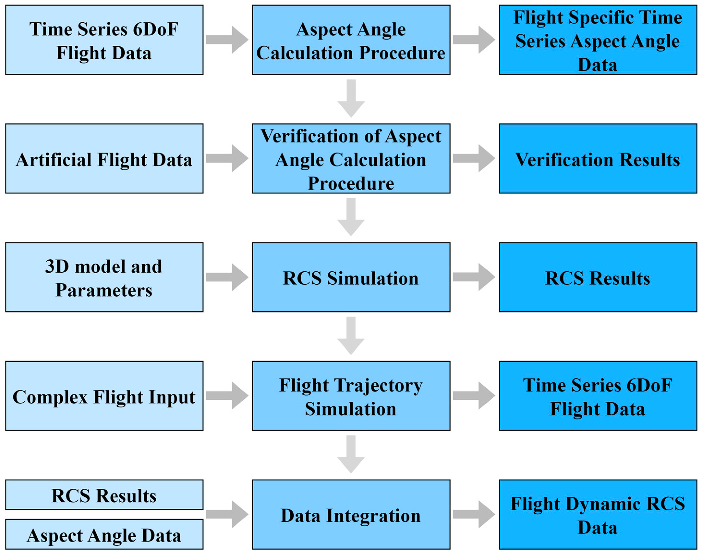
This study proposes an application domain for the aspect angle estimation method outlined in [22], integrating aircraft aspect angles with corresponding RCS values at Euler angles. As illustrated in Figure 1, an assessment of the verification of the aspect angle estimation approach is implemented by utilizing a controlled flight dataset, and then, the RCS simulation is conducted for an aircraft. Throughout this process, challenges encountered in implementing the method proposed in [22] are addressed to acquire a usable dataset of aspect angles along a flight trajectory, aligned with the simulated RCS dataset. Furthermore, the commercial flight simulator software, DCS World [23], is employed to generate an intricate and realistic flight time-series dataset. In brief, a highly maneuverable aircraft is flown in a realistic engagement scenario where air surveillance radar is present. Thanks to the freedom of controlling the aircraft in the simulator, numerous turns and roll maneuvers are conducted during the flight. Moreover, to be able to extract the time-series dataset with 6DoF from the flight conducted in the simulator, another commercially available simulation environment, TacView [24], is utilized. The same software can be used for reviewing and monitoring the whole flight, from start to finish. Then, the acquired time series of 6DoF flight data is used as the input of the aspect angle estimation technique. The problems encountered in the verification of the proposed technique are considered, and some modifications are then applied. As a result, aircraft-to-radar aspect angle data are acquired for targeted flights created in the simulator. Ultimately, all acquired data are fused to establish a flight dynamic RCS profile specific to a designated radar location.
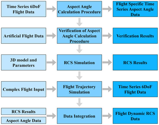
Figure 1.
Flow of the methodology.
The contributions of the paper can be listed as follows:
- We demonstrate the impact of aspect angle on the RCS fluctuations of an aircraft as observed by a ground-based radar threat. To this end, RCS estimation outputs from various flight scenarios were compared and analyzed.
- We investigate the influence of flight dynamics on RCS fluctuations of a UAV-sized aircraft, utilizing readily available tools instead of traditional, costly flight tests or simulations. This demonstrates that practical data through affordable and accessible methods can be acquired.
- We establish an operational framework that may help develop countermeasure strategies, including advanced active decoys.
- We not only evaluate the effect of flight profiles on aspect angles but also thoroughly examine their impact on RCS fluctuations, offering a quantifiable evaluation.
- Our dynamic RCS modeling can be generalized for all engagement scenarios with all operational actors.
The paper is structured as follows: Section 2 describes the aspect angle procedure and verifies its results in the first two subheadings, then discusses the RCS simulation parameters and details of the 3D model used, and finally, details the flight simulation method. Section 3 analyzes the results of the flight simulation characteristics, explains the aspect angle results of the subject flight, and evaluates the RCS fluctuation results obtained from integrating the spherical RCS data of the model and aspect angle data of the simulated flight. Section 4 discusses the methods and results of the paper and outlines future work. Section 5 concludes the paper.
2. Proposed Model for Assessing the Impact of Aircraft Maneuvers on Aspect Angle and RCS Scintillation
2.1. Estimation of Aspect Angle
Aspect angle calculations are conducted following the methodology outlined in [22]. A thorough description of all calculations is provided and elucidated in this section. Subsequently, verification of these calculations is undertaken through artificial flight paths. In these flight paths, the aircraft approaches the radar from the south at an altitude of 3 km. Throughout these control tests, one of the three degrees of freedom—namely, heading, roll, or pitch—serves as the variable, while the others remain constant. Consequently, the impact of varying these attitude variables on the azimuth (θ) and elevation (ϕ) values of the aircraft’s aspect angle can be observed.
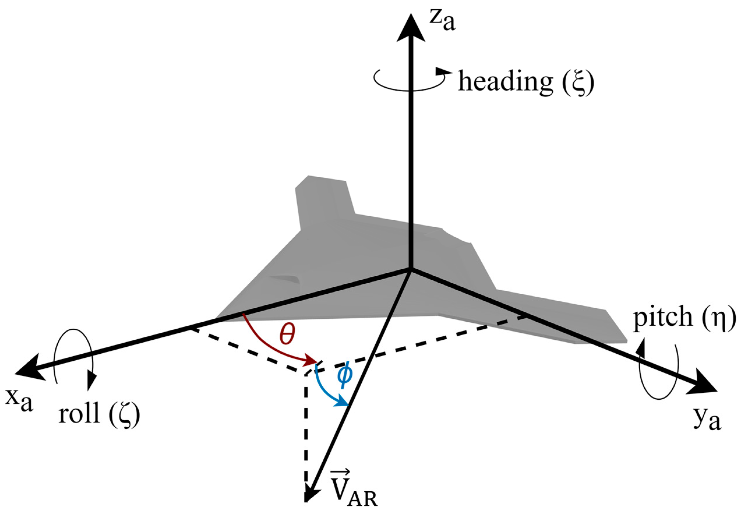
As a first step, we have to assume a coordinate system in which the aircraft is placed in the center, as shown in Figure 2. The x-axis points in the direction of the nose of the aircraft, the y-axis points in the direction of the wing port, and the z-axis points up, perpendicular to the x and y axes. points from the aircraft to the radar and can be expressed as in (1). Thus, the aspect angles θ and ϕ can be calculated as in (2) and (3), respectively.
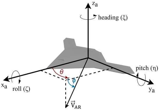
Figure 2.
Illustration of aircraft aspect angles (θ: azimuth ϕ: elevation). Drone model is courtesy of [25].
To determine the arrival angle of the radar beam with respect to the aircraft, the radar-to-aircraft engagement vector () must be found. The aircraft’s position with respect to the radar is expressed as the range (Rng), azimuth (Az), and elevation (El) in the coordinate system of the radar. To map it to the aircraft’s coordinate system, a transformation is carried out. The Rng, Az, and El parameters are transformed into the east, north, and ip coordinate system referenced to the radar as follows:
Thus, can be defined in the Cartesian coordinate system as a result of this first transformation as follows:
The transformation of the radar-to-aircraft vector into the aircraft-to-radar vector can be achieved through its additive inverse as follows:
The radar’s coordinate system, defined by its x, y, and z axes, needs to be transformed into the aircraft’s coordinate system, which comprises the xa, ya, and za axes. After resolving the respective location problem using the , three features in 6DoF are addressed. Now, the integration of the remaining three features—heading, roll, and pitch—into the transformation of into finalizes the estimation technique. The transformation matrix is detailed on a step-by-step basis, addressing each rotation individually. First, the heading (ξ) is investigated in the calculation process. Since the aircraft does not rotate in the z-axis while changing its heading, the x and y axes are subject to the rotation matrix, as depicted in (7). It should be noted that since the ξ angle is referenced to the north, whereas the x-axis of the radar’s coordinate system aligns with the east, a new angle, ξ′, must be utilized (ξ′ = ξ − 90°). This adjustment will be examined during the algorithm’s verification.
The second parameter to be handled is the pitch (η), during which the aircraft rotates its wing port. In this case, the y′-axis remains stable while the x′ and z′ axes rotate, as described in (8)
Finally, the roll angle (ζ) is addressed, during which only the y″ and z″ axes undergo change, as indicated in (9).
All transformation matrices provided in (7), (8), and (9) can be consolidated into one matrix, encapsulating the entire transformation process, as clearly shown in Equation (12) in [22]. As stated at the outset of this sequence of transformation calculations, the primary objective was to derive from . With the transformation matrix identified in [22], can be obtained, as outlined in (10).
Substituting each component of into (2) and (3) culminates in the finalization of the aspect angle calculation, whereby the θ and ϕ angles are expressed exclusively in terms of the 6DoF parameters derived from any flight trajectory data. However, prior to the utilization of intricate flight data as input, supervised flights are imperative to validate the algorithm’s outputs. To this end, the algorithm undergoes trials against an artificial flight trajectory meticulously constructed to serve as a controlled path, enabling the prediction of the aspect angle algorithm’s outputs. Within this trajectory, the aircraft’s commencement from a position 25 km south of the ground radar, with its nose oriented toward the north, thus establishing a heading of 0°, is a foundational premise. Subsequently, the aircraft proceeds with a level flight at a constant altitude until reaching the ground location of the radar. This experimental setup is shown in Figure 3.
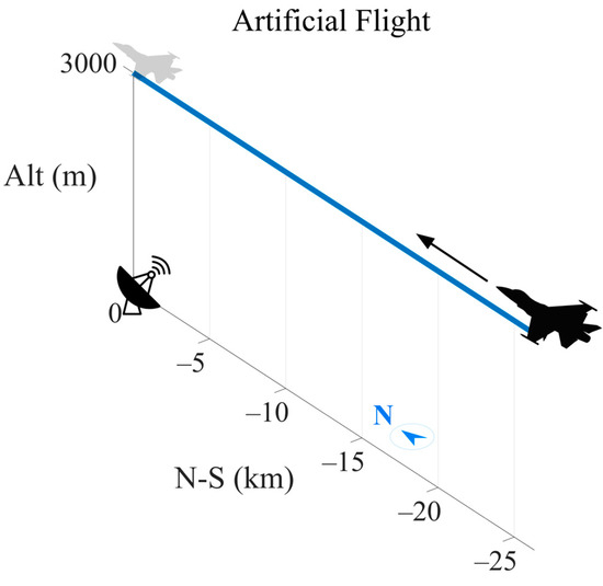
Figure 3.
An artificial flight route is created in MATLAB. Aircraft approaches the radar from the south at a constant velocity.
2.2. Verification of Aspect Angle Calculation Procedure
For the initial phase of verification, the heading angle of the aircraft is systematically adjusted while keeping other angles constant. However, upon examination of the flight path, it becomes evident that deviations from the 0° heading result in the aircraft flying at skewed, unrealistic angles, largely unrelated to the intended flight direction, as illustrated in Figure 4.
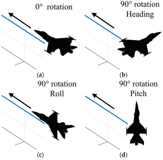
Figure 4.
Verification flights on synthesized path with 0° of rotation in any axis (a), 90° rotation in heading (b), 90° rotation in roll (c), and 90° rotation in pitch (d).
Consequently, this adjustment is expected to induce changes in the azimuth angles of the aircraft’s spherical reference system, allowing for their determination. Ideally, these changes should manifest as a full 0° to 360° circle. However, the results of the calculations present a discrepancy. Specifically, variations in the heading angle result in changes in azimuth, but improper mapping between angles is observed. Upon closer inspection, it is revealed that this pattern arises from the alteration of the ξ angle, as discussed in the initial stages of attitude angle transformation matrix calculations. Surprisingly, in the context of this study, the modification of ξ proves unnecessary and is consequently omitted to attain more precise azimuth angles. The resulting angles are utilized for all subsequent verifications and discussions. Furthermore, another anomaly encountered during the trials is observed beyond 180° azimuth angles, wherein the azimuth angles cease to correspond with the heading angles and instead revert back to 0°, following the same pattern. This phenomenon yields a symmetric chart for azimuth, as depicted. Consequently, any analysis reliant on these angles fails to discern the right or left side of the aircraft. While this presents a challenge for RCS studies, particularly if the aspect angle suggests multiple possible attitudes of the aircraft, it can be overlooked if the RCS profile is symmetrical along the body axis and the primary objective of the study is the expected RCS value, rather than the precise attitude of the aircraft. This pragmatic approach is adopted within this paper. However, it is worth noting that elevation angles show no such inconveniences, with 0° corresponding to wing level, 90° pointing towards the top, and −90° pointing towards the bottom of the aircraft.
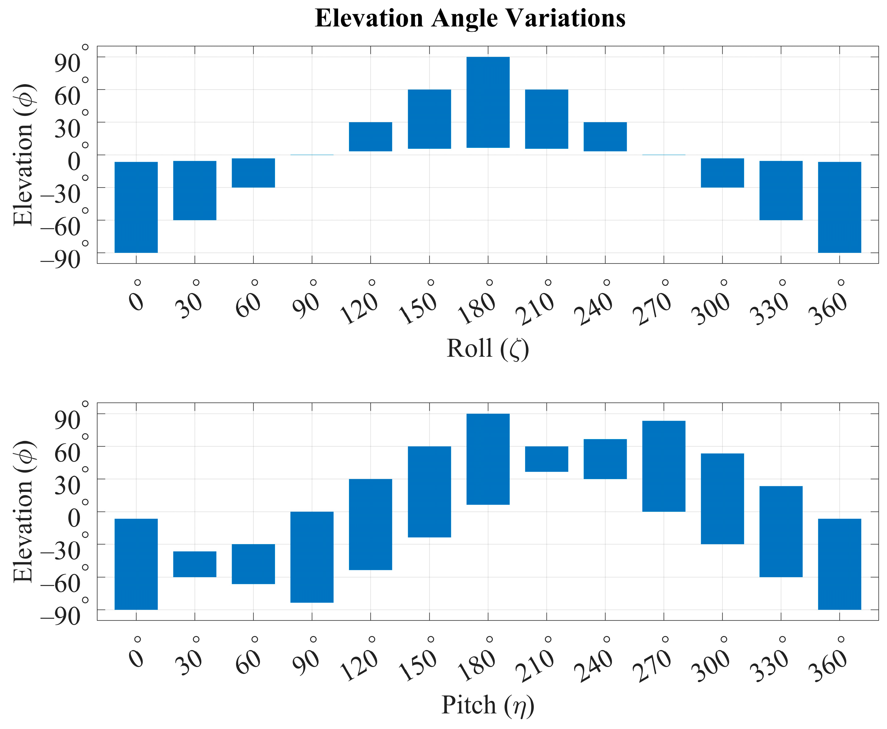
Next, the roll angle is varied to observe its effects on the azimuth and elevation angles. In this experiment, the aircraft is rotated along its roll axis in the same manner as the heading adjustment, as seen in Figure 4, and the resulting changes in azimuth and elevation are examined. Upon reviewing Figure 5, it is expected that when the roll angle is 0°, the azimuth remains constant at 0° because it runs parallel to the surface with no vertical component, while the elevation angle is anticipated to change from a very small value to 90°, given that the starting point of the flight is distant from the radar and the ending point aligns exactly with the z-axis of the radar. In the subsequent step, when the roll is selected to be 30°, both the azimuth and elevation planes no longer remain parallel to the surface and exhibit a vertical component in the radar’s coordinate system. So, at the beginning of the flight, the azimuth angle starts with small values and eventually reaches 90° for every roll rotation value. For each 30° of roll angle, the elevation ends up with a value 30° greater than expected. Additionally, when the wing plane becomes parallel with the surface, the resulting azimuth angle becomes 0°, as observed at 0° and 90° roll angles.
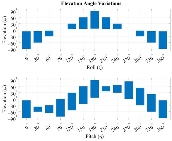
Figure 5.
Variation in elevation angle with respect to roll and pitch angles.
In the third step of the experimental procedure, the pitch angle is systematically adjusted as well. This adjustment is expected to exclusively affect the elevation angle, with notable changes becoming apparent as the aircraft approaches the end of its flight path, specifically at the location of the radar. Notably, as the pitch angle surpasses 90°, azimuth changes are anticipated due to the aircraft effectively traveling backward. The findings presented in Figure 5 illustrate a direct correlation between the increase in pitch angle and the corresponding adjustment in the elevation angle, consistent with theoretical expectations. The narrow results seen at 30°, 60°, 210°, and 240° are actually due to the symmetric structure of the spherical elevation angle axis. For instance, at the beginning of the flight, for a 30° pitch rotation, the elevation angle is at −36.5°; in the middle of the flight, it reaches −90°; and it ends up at −60°, thus the angle interval scanned throughout the flight is constant at each pitch angle. This observation reinforces the notion that pitch adjustments predominantly influence the elevation angle during aircraft maneuvers.
2.3. Radar Cross-Section (RCS) Simulations
For the RCS simulation, an open-source three-dimensional approximate model of a fighter jet is employed and a custom code is executed for RCS simulations [26]. Due to challenges in selecting a suitable UAV/UCAV model for simulations, priority was given to the size of the aircraft. The unavailability of an appropriate UAV/UCAV model necessitated the selection of an alternative aircraft with a similar geometry. On the other hand, given the high speeds and maneuverability exhibited by the new generation of UAV/UCAVs, the employed fighter jet model presents itself as a potentially suitable model for RCS analysis. Furthermore, the methodology of this study is adaptable and can be applied to various models and platforms. Table 1 summarizes the specifications of the aircraft and computation parameters. The RCS computation is conducted in the L-band frequency region (1.4 GHz). The PO technique is utilized for the simulation because of the large dimensions of the model and high-frequency application, as well as low hardware demand and short run times [27]. Following the λ/10 criterion, the 3D model undergoes a perfect electric conductor (PEC) meshing operation with triangles of 0.02 m edge length prior to the RCS simulation, resulting in 878,284 triangles comprising the external surface of the jet platform. The results are obtained across the 360 degrees of azimuth and elevation of the model with 1° steps.

Table 1.
Summary of RCS simulation features.
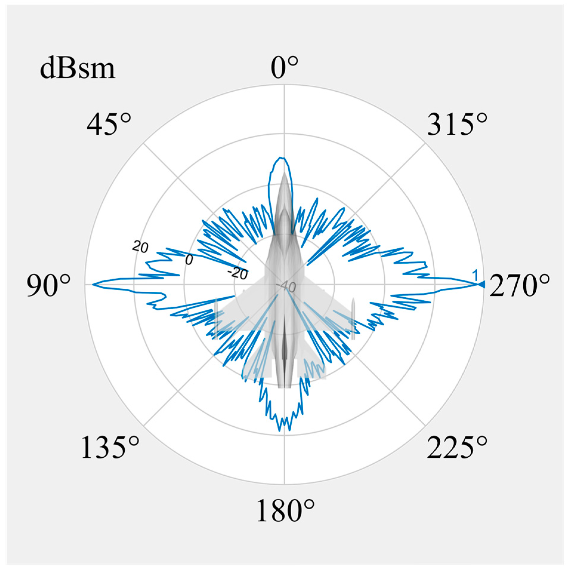
A full circle RCS result of the 3D model at 0° elevation (ϕ) is depicted in Figure 6. In the radial azimuth plot, the aircraft’s nose corresponds to θ = 0° and the RCS values show peaks at the nose, wing tips, and tail of the aircraft. Since physical optics (PO) calculations may sometimes introduce inaccuracies when a model has deep dents and reflectors and due to imperfections in the 3D model, some asymmetric results could be observed; whereas the RCS signature is expected to be approximately symmetric along the body of the aircraft. To evaluate these inconsistencies, the outcomes were compared with those for similar aircraft models from [28,29] and were found to be mostly consistent. The peaks valued at 36 dBsm at 90° and 270° of the radial plots are likely due to cylindrical shapes on the wing tips and missiles mounted under the wings. The 18 dBsm peak at 180° is presumably attributed to the engine exhaust meshing in the model, which acts like a corner reflector. Additionally, the air inlet under the nose is probably responsible for the peak at 0°, which is just over 10 dBsm at its maximum in between 9° and 356° degrees of azimuth. Generally, the RCS results are greater than 0 dBsm once in every 90° from the nose of the aircraft for certain angle intervals. The highest peaks are present at the wing tips, specifically between 73° and 101° for the left side and between 287° and 259° for the right side. Peak values at the rear are located between 189° and 166° at the azimuth.
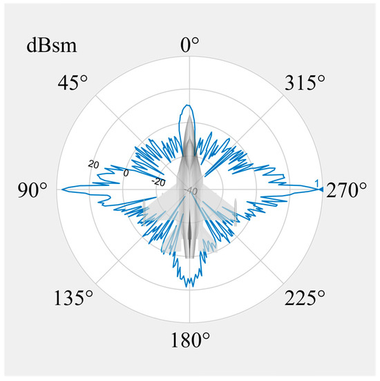
Figure 6.
RCS result of the model at 0° elevation and 0–360° azimuth. For reasons of availability, a more accessible model is used for the simulations.
2.4. Flight Trajectory Simulation
While 6DoF parameters of aircraft motion can be derived for straightforward flight trajectories such as level flight, sustained turns, and straight takeoff and landing, generating complex flight path data is essential for a realistic engagement scenario in a battlefield. To achieve this, the use of flight simulator software is necessary, given that the classification policies of armed forces worldwide strictly maintain the confidentiality of datasets and do not disclose them to the public. Additionally, developing a dataset entirely in-house facilitates the usability of the final product and allows for seamless integration within its intended scope.
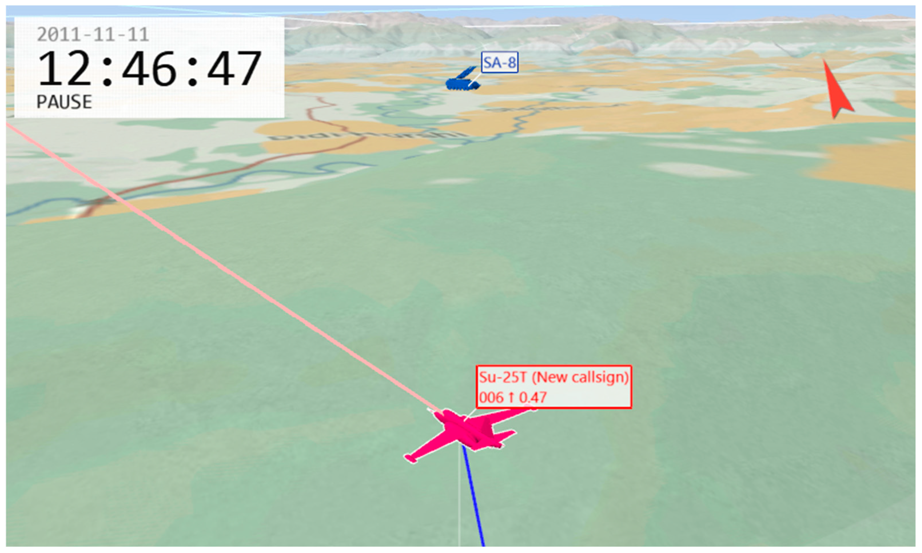
A commercial simulation software, namely, “Digital Combat Simulator (DCS World)” [23], served as the platform for generating intricate and realistic flight paths within a threat-platform scenario. In this scenario, the threat is represented by a fixed land radar with a known position, as depicted in Figure 7. At the onset of the flight, a fixed-wing platform embarks from the farthest end of the blue-colored path relative to the radar position. Throughout the flight, various maneuvers are executed to induce changes in roll, pitch, and heading angles. A representative sortie, depicted in Figure 7, is conducted for this study, during which the aircraft traverses along the blue path while dynamically adjusting its attitude through rotations. Upon completion of the flight, all 6DoF parameters are extracted using a flight data analysis tool, TacView [24], with a sampling rate of 1 Hz. Leveraging the 3D scene viewing capabilities of this tool, the entire flight scene is scrutinized to verify aspect angles through direct observation, as seen in Figure 8.
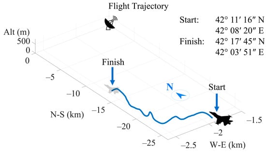
Figure 7.
Flight path of the aircraft (blue string) and position of the radar.
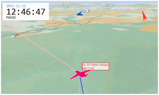
Figure 8.
A moment from flight seen on TacView software. Su-25T aircraft is used to create flight trajectory due to availability reasons and it is anticipated that no significant differences exist between the flight characteristics of different aircraft under study. SA-8 represents the location of the radar.
3. Results
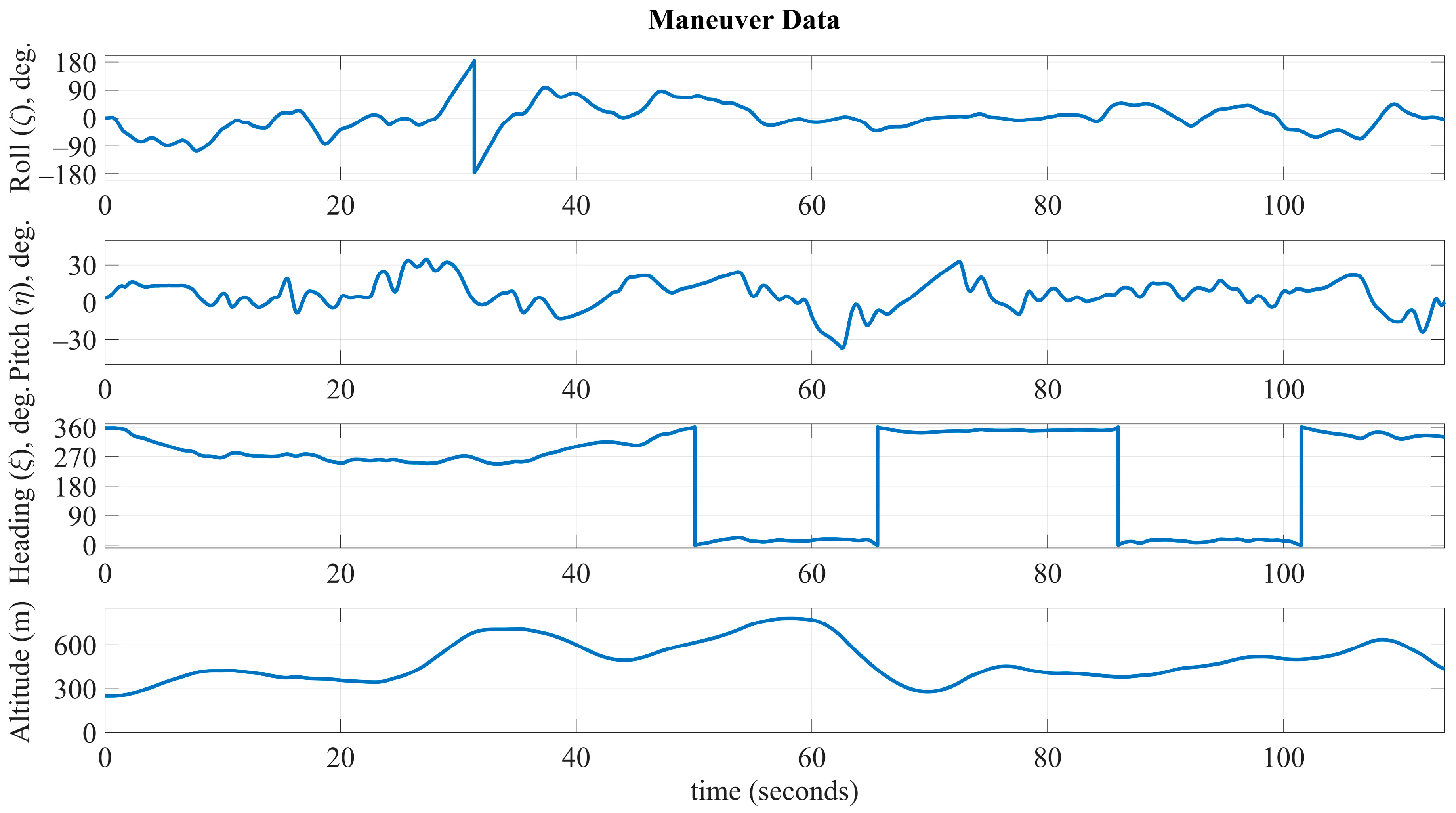
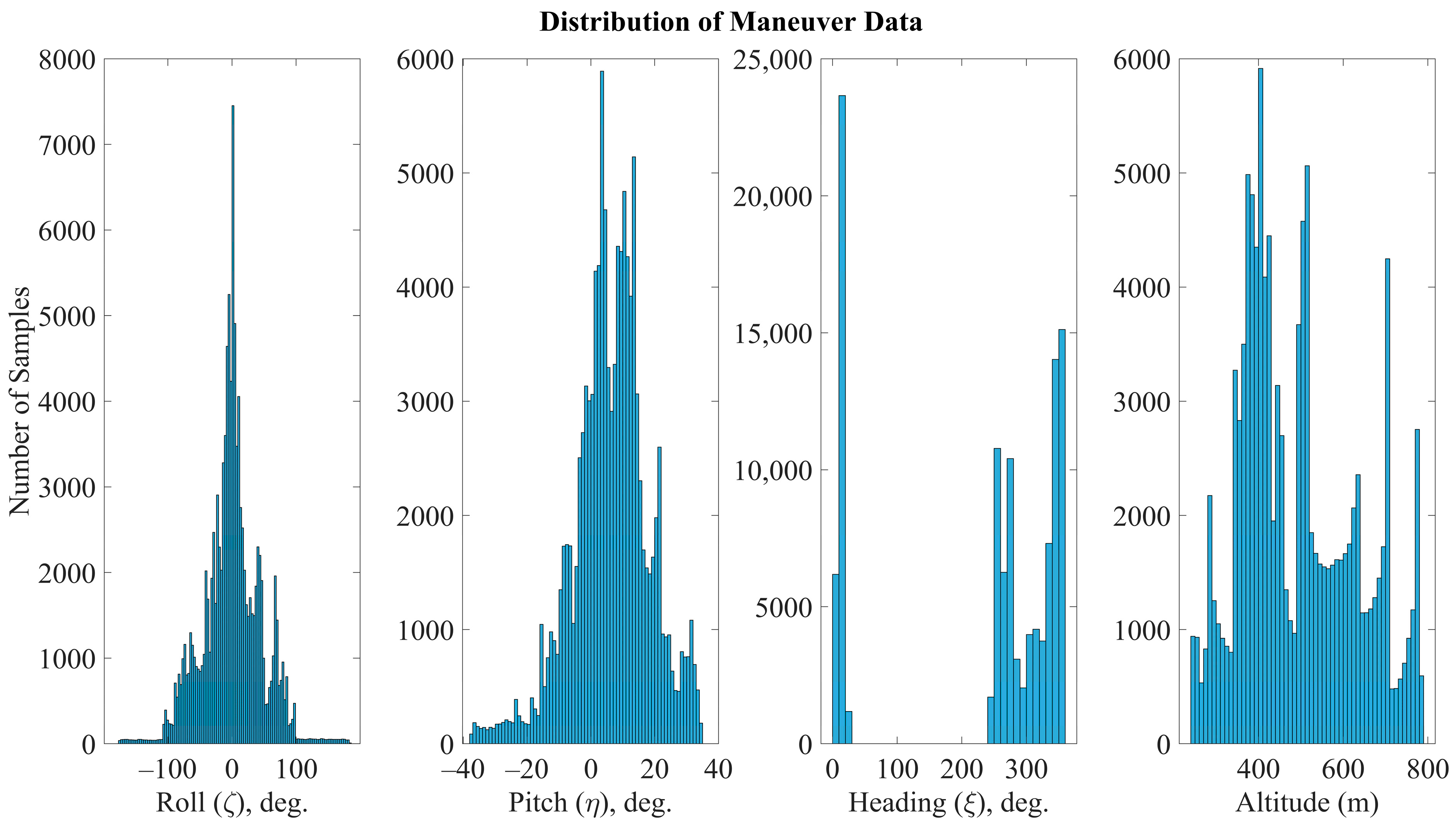
The RCS results were derived using a spherical scope of a 3D aircraft model, as opposed to the cylindrical model employed in [12], where RCS was simplified for roll maneuvers. This method highlighted the roll angle’s significant impact on RCS fluctuations throughout the flight, enabling the simulation of aircraft movements to closely mimic real-world scenarios and not confining the analysis to a few specific flight modes as in [15]. However, implementing the aspect angle calculations from [22] for this study revealed several challenges in integrating the two datasets. To address the azimuth angle output issue—where the algorithm produced values only between 0° and 180°, and sometimes negative elevation values—assumptions of symmetry in the platform RCS were made. An orientation process was subsequently implemented to align the RCS values with the correct angles during data integration. Dynamic flight RCS data for the aircraft were gathered using accessible and cost-effective data acquisition methods, unlike in [16], which used real INS data and uniform flight patterns across various aircraft, for which the attitude angles are minute. Essential characteristics of the flight data obtained from the flight simulator are detailed in Figure 9, where angular degrees of freedom and altitude values throughout the flight are plotted. The sudden drop in the ζ value around the 30 s mark results from a 360° roll maneuver. Aside from that, the aircraft generally remained parallel to the ground most of the time. As seen in Figure 10, the roll angle instances create a normal distribution centered around 0°. Sharp falls and rises in the heading (ξ) plot indicate transitions between 0° and 359° on the compass, rather than an unrealistic rotation on the compass plane. Between the 10 and 40 s marks, the nose of the aircraft generally pointed towards the west, resulting in 270° data values during that interval. Pitch (η) values are not sharply accumulated around the 0° mark like ζ, as the aircraft tends to point upwards, leading to a high number of instances around the 10° mark. Generally, samples are distributed between 0° and 20°. For a stable flight, all these parameters are supposed to peak at one point. However, in this case, the aircraft is quite maneuverable and utilizes this ability in an engagement scenario, thus the plots show variability in complex flight scenarios.

Figure 9.
Flight specific degrees of freedom and altitude values with respect to flight time.

Figure 10.
Instance distributions of degrees of freedom and altitude values of the flight.
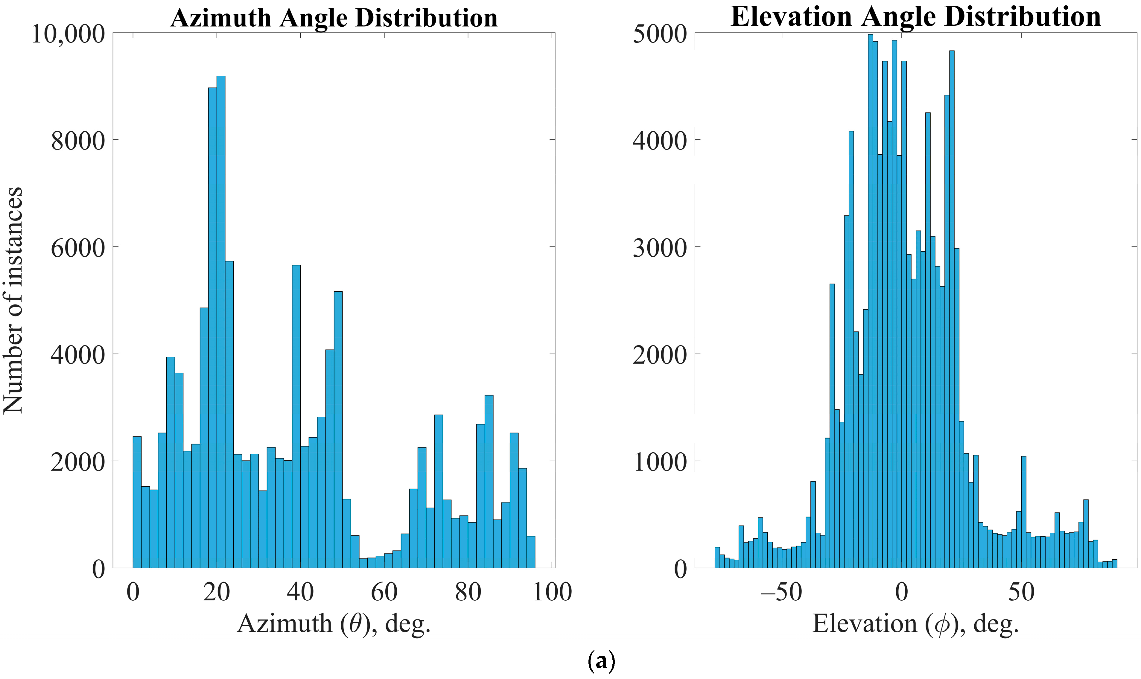
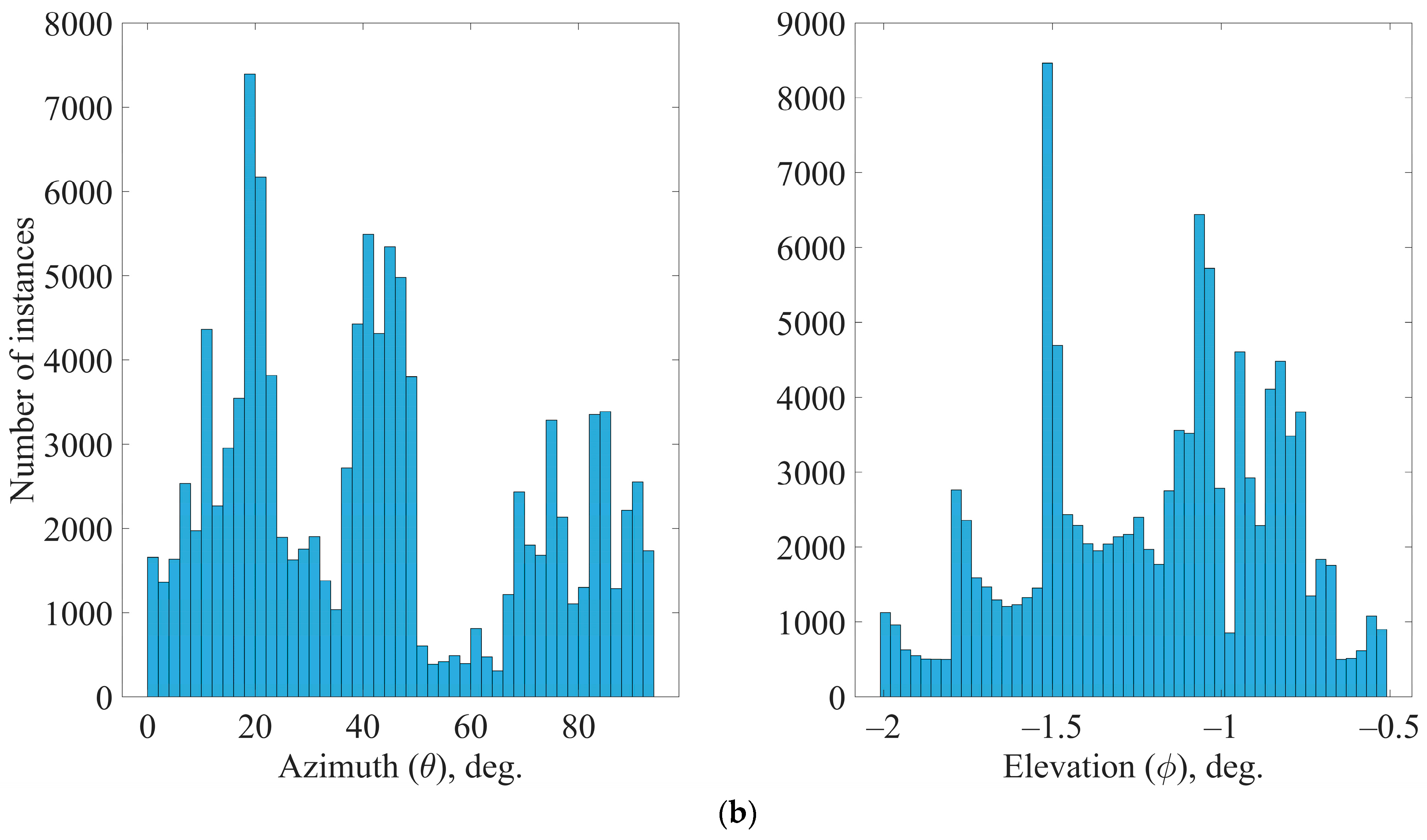
The azimuth aspect angle calculations resulted in a more dispersed data cluster compared to the data found in [16], as shown in Figure 11. Due to the radar’s position near the north-northeast of the aircraft, the azimuth aspect angle values accumulated in two intervals: 0–50° and 65–80°. The aircraft predominantly flew northward, leading to accumulation in the 0–50° range, while eastward flights caused the 65–80° interval to capture the remaining instances. The elevation values were predictable and comparable with [16] because the aircraft’s bottom pointed down for most of the flight. Despite some extreme roll angle values, the roll angle peaked near 0°, as seen in Figure 10. When roll and pitch angles were ignored and set to zero throughout the flight, resulting in a flight conducted solely with heading and altitude changes, the azimuth results did not change significantly, maintaining clear grouping. The elevation aspect angle values vary between −2° and −0.5°, contrasting with the −90° to 90° range seen in the fully disturbed data, demonstrating the significance of rotational degrees of freedom on aspect angles.
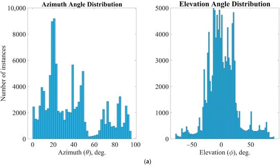
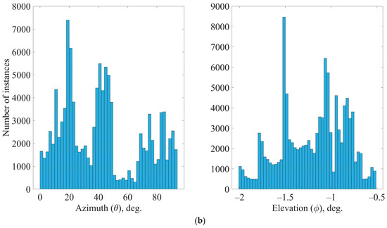
Figure 11.
Aspect angle distributions of two different flight data, (a) represents azimuth and elevation distributions of the flight data with full disturbance, (b) represents the azimuth and elevation distributions of flight data with zero roll and pitch rotation.
The effect of the flight profile on aspect angles is given in Table 2. It is important to note that the cases in [16] disabled all degrees of freedom, including heading, while in this paper, only roll and pitch are disabled. The rotation in heading significantly affects aspect angles in the case of this paper, so reaffirming this was deemed unnecessary. Additionally, the heading angle variation in [16] was minimal, making the disabling of the heading variable closely align with real data. In contrast, the data used in this paper show significant changes in heading, and setting it to zero would result in unrealistic flight profiles, such as an aircraft traveling west while its nose points north, and overall, causing incomparability with the data provided in [16]. To avoid this, heading was not altered primarily, allowing for direct comparison of elevation, which is independent of the heading parameter. Moreover, while in [16] the azimuth scale includes negative values, this paper scales azimuth between 0° and 180°. This difference is manageable and does not significantly impact the analysis. The major difference in the maximum value of elevation is expected since it is largely dependent on roll and elevation. Regardless, if heading is set to zero, the gap between the maximum and median value of the azimuth aspect angle becomes narrow, indicating that the variation only depends on the location of the aircraft and relative distance to the radar, while the rotational effect plays an important role in data with full disturbance.
Table 2.
Comparison of effect of flight profiles on variation in aspect angles.
Following the acquisition of the two datasets, namely, the RCS simulation results and aspect angle calculations, they are finally integrated to elucidate the radar-specific RCS behavior of the aircraft, as seen in Figure 12, visualizing the RCS scintillation level of the platform on the radar throughout the flight time, and some of these fluctuation behavior changes at the highlighted points are observed in the TacView [24] flight monitor at the corresponding time. At point A, the aircraft makes a roll and pitch maneuver, resulting in only showing the bottom of the body with a skewed angle. At point B, another roll maneuver is made suddenly and the RCS is reduced drastically, which can also be seen at point C, where a 360° roll maneuver is conducted. After 40 s, the aircraft goes into a more stable flight profile, attempting less attitude changes. Lastly, at point D the plane turns its nose slightly towards the radar, resulting in a little peak in the flight dynamic RCS profile. Furthermore, the RCS fluctuation results derived from the flight data depicted in Figure 11, where the roll and pitch angles were zeroed, are presented using the blue line. Beyond the annotated points, numerous instances exhibit significant deviations of varying magnitudes. Towards the end of the flight, a notable divergence is observed, with the blue line peaking near 15 dBsm, contrasting sharply with the red line, which shows a marked decrease to approximately −25 dBsm. Another distinct disparity appears around the 47 s mark, with an RCS difference of nearly 30 dBsm evident. Overall, the flight data reflecting realistic conditions with full degrees of freedom display a more dynamic RCS profile, while the constrained dataset results in a less volatile and less unstable RCS scintillation. Although a detailed analysis and evaluation of the major differences between the two RCS datasets may reveal more critical insights, the average difference between them is found to be 32.44% when using the full-disturbance RCS as the reference.
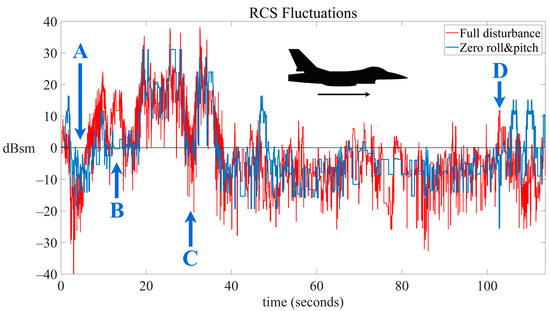
Figure 12.
RCS fluctuation data from the view of the radar with respect to time. Red indicates the data with full rotational degrees of freedom, blue indicates the same data but with zero degrees of roll and pitch rotation. Points A (2.–5. s), B (11. s), C (29.–32. s), and D (103. s) indicate significant changes in RCS appearance of the aircraft during flight.
As illustrated in Figure 13, fluctuations in the RCS are discernible along the flight path. Notably, these fluctuations are intricately tied to the specific location of the radar. It is imperative to note that even if the flight path remained unaltered, variations in the observer’s position would yield entirely different RCS fluctuations. In essence, the red plot delineates the exposure level of the radar throughout the duration of the flight, serving as a comprehensive representation of the radar’s interaction with the aircraft.
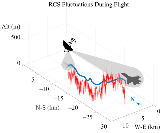
Figure 13.
RCS amplitude plot of the aircraft precisely mapped along the flight route (blue). RCS fluctuations seen from the location of the radar at the origin (red).
The results of the study show that the methodologic approach utilized near-realistic, accessible and repeatable simulations to depict RCS fluctuation behavior under dynamic flight conditions. The effects of the degrees of freedom are analyzed by comparing the statistics of different flight profiles and RCS scintillation results of the aspect angles.
4. Discussion
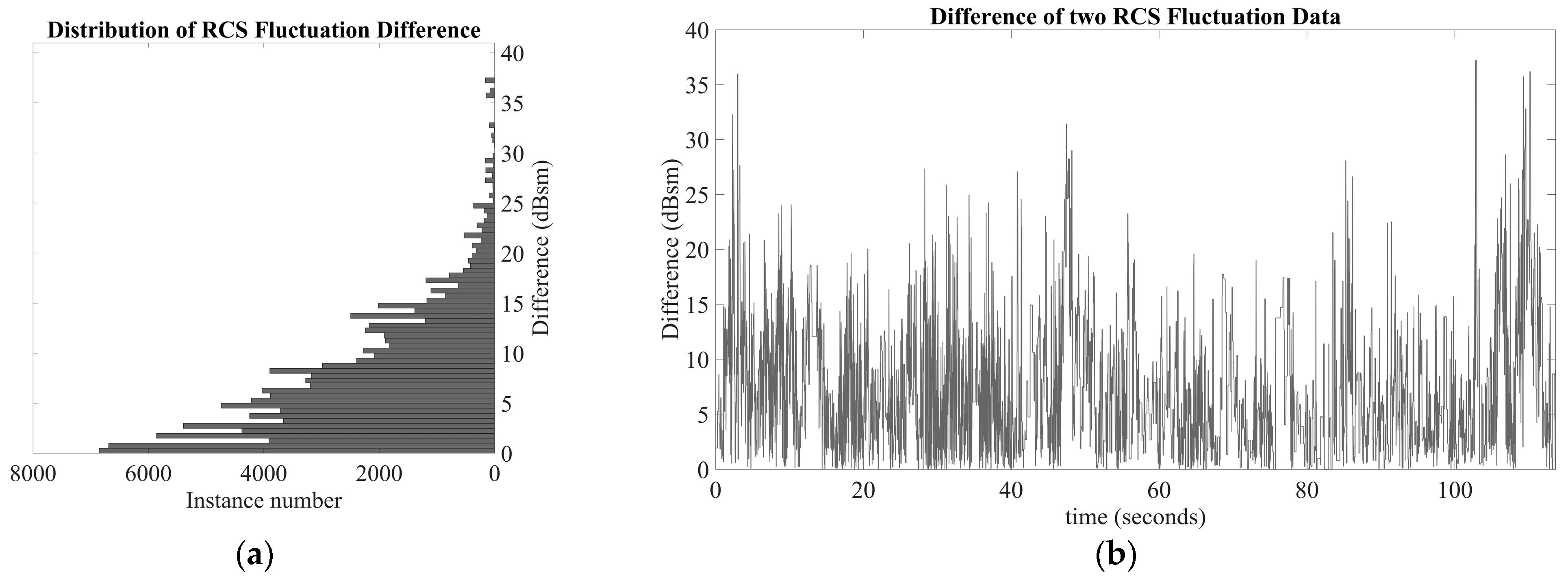
The aim of this paper was to propose and utilize a set of methods to ascertain the impact of rotational degrees of freedom on the RCS scintillation of a UAV observed from a ground radar. The review of the existing literature highlights a gap in affordable and accessible solutions for generating necessary flight data in a user-friendly and repeatable manner, prompting this paper to advocate for the use of commercial flight simulators and monitoring software in the process. The RCS simulation process employed here includes only PO calculations due to their computational efficiency and minimal hardware demands. Given the extended duration of each simulation step, RCS calculations are conducted at every degree of the aircraft’s azimuth and elevation. While it is feasible and potentially advantageous to perform RCS calculations using alternative methods such as MoM or SBR with more frequent intervals, the current approach balances precision and computational feasibility. Although the λ/10 triangulation criterion is deemed adequate, reducing this value would likely enhance the accuracy of the RCS calculations. The quality of RCS calculations is inherently dependent on the chosen method and model, which are significantly influenced by the available hardware and software tools. The aspect angle calculation procedure was verified using supervised flights generated with a custom code, yielding satisfactory results. Consequently, further verification with other simulation software or another framework is not deemed necessary. However, developing a versatile simulation script within a simulation framework could reduce errors and the time spent on validating aspect angle results with other monitoring software. The methods outlined in this paper are sufficient for the current scope of interest, but high-sensitivity and large-scale analyses may require more sophisticated customizations, particularly for evaluating the effectiveness of countermeasures. There is a challenge in statistically analyzing the differences between two RCS datasets that exhibit similar overall trends but contain significant discrepancies at certain points. Conducting a detailed maneuver analysis to understand these variations is complex and beyond the scope of this paper, but it is a crucial subject for future research. The comparison metrics presented in Figure 13 include both overall differences and time-dependent variations. Figure 14 quantifies these differences, providing a numerical summary. Determining the threshold for what constitutes a critical dBsm difference is highly context-dependent, varying according to specific engagement scenarios and operational considerations. Therefore, making a definitive judgment on whether the maneuver significantly impacts the RCS is not within the scope of this study. Instead, this paper lays the groundwork for understanding the basic trends and highlights the need for more in-depth analysis in future work.

Figure 14.
Difference in two RCS scintillation values. (a) shows the number of difference values; (b) shows the difference in RCS outputs as a time series.
In future research endeavors, a focused exploration into refining aspect angle calculations could significantly enhance the depth and accuracy of our understanding within the context of this study. By delving into the intricacies of aspect angle tuning, researchers could propose innovative methodologies or adjustments aimed at improving the precision and reliability of these calculations. Moreover, there exists ample opportunity to elevate the quality of RCS simulations by leveraging more sophisticated 3D models and advanced hardware capabilities. By employing state-of-the-art technology and techniques, such as higher-fidelity modeling and superior hardware configurations, researchers can strive to achieve more accurate and detailed RCS simulations, thereby providing deeper insights into the dynamic interactions between aircraft and radar systems. Also, with the rapid advancement of cognitive radar technology showing significant improvements in target tracking [17], traditional active decoys are at risk of becoming outdated due to the superior processing and adaptive capabilities of cognitive radar systems in military applications. To counteract the sophisticated feedback mechanisms that allow cognitive radars to sense, learn, and adapt to their environment [19], it is essential to upgrade active decoy algorithms and functionalities. These decoys need to be more dynamic and responsive. Utilizing the RF properties of the aircraft deploying the decoy can offer valuable inputs for enhancing and fine-tuning the decoy’s jamming capabilities. These advancements hold the potential to enrich our understanding of dynamic combat scenarios and contribute to the development of more effective defense strategies in the future.
5. Conclusions
This study aimed to investigate the influence of flight dynamics on RCS fluctuations of a UAV-sized aircraft as detected by ground-based radar, utilizing readily available tools in place of conventional restrictive demonstrations, expensive flight tests, or simulations. The goal was to create a framework for operational analysis and develop countermeasure strategies such as advanced active decoys. An interactive simulation environment was employed to gather flight data, with the aircraft’s aspect angles relative to the ground radar calculated to obtain relevant azimuth and elevation angles over time, resulting in a comprehensive time-series dataset. Through post-operation monitoring, significant RCS fluctuations were identified and linked to specific aircraft maneuvers by observation. The analysis highlighted the crucial role of flight maneuvers, demonstrating that dynamic changes in roll and pitch can lead to RCS fluctuations exceeding 35 dBsm in the case of this study. Utilizing advanced modeling techniques, this research provides insights into the complex relationship between flight maneuvers and RCS behavior, with an emphasis on the influence of roll and pitch angles. By combining aspect angle calculations with simulated RCS data, this study contributes to future defense and countermeasure research. Especially in the areas of advanced active decoys which can emulate platform RCS fluctuation, and cognitive radar technologies which can utilize learning algorithms, offering valuable implications for future warfare concepts.
Supplementary Materials
Custom MATLAB scripts and 3D model used in this paper can be found at: https://github.com/senkrm/aspect-angle-specific-rcs (accessed on 13 September 2024).
Author Contributions
Conceptualization and methodology K.S., A.K. and S.A.; investigation, software, validation, visualization, and writing—original draft K.S.; supervision and writing—review and editing S.A. and A.K. All authors have read and agreed to the published version of the manuscript.
Funding
This research received no external funding.
Data Availability Statement
Custom MATLAB scripts, 3D model and the dataset used in this paper (Supplementary Materials) can be found at: https://github.com/senkrm/aspect-angle-specific-rcs (accessed on 13 September 2024).
Acknowledgments
This work is supported by ASELSAN Inc. The authors would like to thank ASELSAN Inc.
Conflicts of Interest
Authors Kerem Sen and Sinan Aksimsek were employed by the company ASELSAN Inc. The remaining author declares that the research was conducted in the absence of any commercial or financial relationships that could be construed as a potential conflict of interest.
References
- Bianchi, D.; Borri, A.; Cappuzzo, F.; Di Gennaro, S. Quadrotor Trajectory Control Based on Energy-Optimal Reference Generator. Drones 2024, 8, 29. [Google Scholar] [CrossRef]
- Gui, D.; Le, M.; Huang, Z.; D’Ariano, A. A Decision Support Framework for Aircraft Arrival Scheduling and Trajectory Optimization in Terminal Maneuvering Areas. Aerospace 2024, 11, 405. [Google Scholar] [CrossRef]
- Deng, H.; Huang, J.; Liu, Q.; Zhao, T.; Zhou, C.; Gao, J. A Distributed Collaborative Allocation Method of Reconnaissance and Strike Tasks for Heterogeneous UAVs. Drones 2023, 7, 138. [Google Scholar] [CrossRef]
- Guan, J.; Huang, J.; Song, L.; Lu, X. Stealth Aircraft Penetration Trajectory Planning in 3D Complex Dynamic Environment Based on Sparse A* Algorithm. Aerospace 2024, 11, 87. [Google Scholar] [CrossRef]
- Leonardo, S.p.A. RAT 31DL L-Band/Solid State 3D Air Surveillance Radar. Available online: https://electronics.leonardo.com/en/products/rat-31dl (accessed on 27 February 2024).
- Uluisik, C.; Cakir, G.; Cakir, M.; Sevgi, L. Radar Cross Section (RCS) Modeling and Simulation, Part 1: A Tutorial Review of Definitions, Strategies, and Canonical Examples. IEEE Antennas Propag. Mag. 2008, 50, 115–126. [Google Scholar] [CrossRef]
- Ling, H.; Chou, R.-C.; Lee, S.-W. Shooting and Bouncing Rays: Calculating the RCS of an Arbitrarily Shaped Cavity. IEEE Trans. Antennas Propag. 1989, 37, 194–205. [Google Scholar] [CrossRef]
- Weinmann, F. Ray Tracing with PO/PTD for RCS Modeling of Large Complex Objects. IEEE Trans. Antennas Propag. 2006, 54, 1797–1806. [Google Scholar] [CrossRef]
- Sezgin, D. Radar Cross Section Measurement of Various Objects with 77–81 GHz Automotive Radar and Assessment of Radar Cross Section Simulation Tools. Master’s Thesis, Atılım University, Ankara, Türkiye, 2022. [Google Scholar]
- Wolff, C. Radar Cross-Section. Available online: https://www.radartutorial.eu/ (accessed on 27 April 2024).
- Fourikis, N. Advanced Array Systems, Applications and RF Technologies; Signal Processing and Its Applications; Academic Press: San Diego, CA, USA, 2000; ISBN 978-0-12-262942-6. [Google Scholar]
- Hu, Y.; Qi, X.; Cao, R.; Liu, B.; Yang, K. Research on Relationship between RCS of Moving Targets and Radar Aspect Angle. In Proceedings of the 2022 IEEE 5th Advanced Information Management, Communicates, Electronic and Automation Control Conference (IMCEC), Chongqing, China, 16–18 December 2022; IEEE: Chongqing, China, 2022; pp. 1848–1857. [Google Scholar]
- Zhang, Z.; Jiang, J.; Wu, J.; Zhu, X. Efficient and Optimal Penetration Path Planning for Stealth Unmanned Aerial Vehicle Using Minimal Radar Cross-Section Tactics and Modified A-Star Algorithm. ISA Trans. 2023, 134, 42–57. [Google Scholar] [CrossRef] [PubMed]
- Xu, Q.; Ge, J.; Yang, T.; Sun, X. A Trajectory Design Method for Coupling Aircraft Radar Cross-Section Characteristics. Aerosp. Sci. Technol. 2020, 98, 105653. [Google Scholar] [CrossRef]
- Herman, S.M. Joint Passive Radar Tracking and Target Classification Using Radar cross Section; Drummond, O.E., Ed.; SPIE: San Diego, CA, USA, 2003; pp. 402–417. [Google Scholar]
- Persson, B.; Bull, P. Empirical Study of Flight-Dynamic Influences on Radar Cross-Section Models. J. Aircr. 2016, 53, 463–474. [Google Scholar] [CrossRef]
- Haykin, S.; Zia, A.; Arasaratnam, I.; Xue, Y. Cognitive Tracking Radar. In Proceedings of the 2010 IEEE Radar Conference, Arlington, VA, USA, 10–14 May 2010; IEEE: Arlington, VA, USA, 2010; pp. 1467–1470. [Google Scholar]
- Haifawi, H.; Fioranelli, F.; Yarovoy, A.; Van Der Meer, R. Drone Detection & Classification with Surveillance ‘Radar On-The-Move’ and YOLO. In Proceedings of the 2023 IEEE Radar Conference (RadarConf23), San Antonio, TX, USA, 1–4 May 2023; IEEE: San Antonio, TX, USA, 2023; pp. 1–6. [Google Scholar]
- Guerci, J.R.; Guerci, R.M.; Ranagaswamy, M.; Bergin, J.S.; Wicks, M.C. CoFAR: Cognitive Fully Adaptive Radar. In Proceedings of the 2014 IEEE Radar Conference, Cincinnati, OH, USA, 19–23 May 2014; IEEE: Cincinnati, OH, USA, 2014; pp. 0984–0989. [Google Scholar]
- Knott, E.F.; Shaeffer, J.F.; Tuley, M.T. Radar cross Section, 2nd ed.; Artech House Radar Library; Artech House: Boston, MA, USA, 1993; ISBN 978-0-89006-618-8. [Google Scholar]
- Chen, W.-K. The Electrical Engineering Handbook; Elsevier Academic Press: Amsterdam, The Netherlands, 2005; ISBN 978-0-12-170960-0. [Google Scholar]
- Caraway, W.D.; Abell, D.C. A Method for the Determination of Target Aspect Angle with Respect to a RADAR; US Army Missile Command: Redstone Arsenal, AL, USA, 1996. [Google Scholar]
- Eagle Dynamics, S.A. Digital Combat Simulator. Available online: https://www.digitalcombatsimulator.com/cn/ (accessed on 13 September 2024).
- Raia Software Inc. TacView (1.9.3) 2006. Available online: https://www.tacview.net/download/latest/en/ (accessed on 13 September 2024).
- Northrop Grumman X-47B by 67bope Is Licensed under the Creative Commons—Attribution—Non-Commercial—No Derivatives License. Available online: https://www.printables.com/model/216790-northrop-grumman-x-47b (accessed on 13 September 2024).
- “F-16” (Https://Skfb.Ly/HQxq) by Surveytown Is Licensed under Creative Commons Attribution. 2015. Available online: https://sketchfab.com/3d-models/f-16-00d69679955a423a9337726635cc5e1c (accessed on 13 September 2024).
- Chatzigeorgiadis, F. Development of Code for a Physical Optics Radar cross Section Prediction and Analysis Application. Ph.D. Thesis, Naval Postgraduate School, Monterey, CA, USA, 2006. [Google Scholar]
- Yue, K.; Chen, S.; Shu, C. Calculation of Aircraft Target’s Single-Pulse Detection Probability. J. Aerosp. Technol. Manag. 2015, 7, 314–322. [Google Scholar] [CrossRef]
- Touzopoulos, P.; Boviatsis, D.; Zikidis, K.C. 3D Modelling of Potential Targets for the Purpose of Radar Cross Section (RCS) Prediction: Based on 2D Images and Open Source Data. In Proceedings of the 2017 International Conference on Military Technologies (ICMT), Brno, Czech Republic, 31 May–2 June 2017; IEEE: Brno, Czech Republic, 2017; pp. 636–642. [Google Scholar]


Disclaimer/Publisher’s Note: The statements, opinions and data contained in all publications are solely those of the individual author(s) and contributor(s) and not of MDPI and/or the editor(s). MDPI and/or the editor(s) disclaim responsibility for any injury to people or property resulting from any ideas, methods, instructions or products referred to in the content. |
© 2024 by the authors. Licensee MDPI, Basel, Switzerland. This article is an open access article distributed under the terms and conditions of the Creative Commons Attribution (CC BY) license (https://creativecommons.org/licenses/by/4.0/).