Abstract
Space robots are vital for in-orbit maintenance of large satellites, but dense payloads and complex surface structures pose challenges for safe crawling operations. This study proposes an improved trajectory planning framework for three-dimensional satellite surfaces. In the path search stage, the traditional A* algorithm is enhanced with traction cost, reflecting surface adhesion, and proximity cost, ensuring collision avoidance. The resulting comprehensive cost function integrates path length, safety, and feasibility, producing paths more consistent with real mobility constraints. In the smoothing stage, cubic B-spline curves refine the discrete path, with real-time collision detection embedded in the optimization of control points to prevent trajectory penetration. Simulations show that the method achieves millisecond-level planning, with path length reduced by 6.82% and trajectory smoothness significantly improved, eliminating the phenomenon of sharp turns with folded corners. The approach ensures continuous, stable, and collision-free movement of space robots, highlighting its potential for reliable in-orbit operations.
1. Introduction
In addressing satellite in-orbit issues, space robots serve as highly efficient maintenance tools. Typically deployed aboard large orbital service vehicles, these robots can approach target satellites autonomously or under control. Utilizing biomimetic adhesion technology, they traverse satellite surfaces with stability to execute precision maintenance tasks [1]. However, achieving efficient and reliable autonomous movement across complex topographical features on satellite surfaces remains a challenging problem in path planning. On the one hand, the robot must navigate multidimensional environmental challenges, including varying surface materials and three-dimensional curved surfaces [2]. On the other hand, when performing hull inspections or localized repairs, multiple constraints—including contact stability [3], energy-efficient motion optimization, and obstacle avoidance [4]—must be comprehensively considered to devise safe and efficient movement paths. Current path planning research primarily encompasses traditional classical algorithms, evolutionary computation methods, and swarm intelligence optimization algorithms. Among these, classical algorithms form the theoretical foundation of path planning. For instance, Dijkstra’s algorithm [5] employs a breadth-first strategy to guarantee global optimality but suffers from low computational efficiency. Floyd’s algorithm [6] excels at solving the all-sources shortest path problem. Meanwhile, the APF algorithm [7,8] achieves real-time obstacle avoidance through virtual force fields but is prone to getting stuck in local minima. The RRT* [9] progressively approximates optimal paths through parent node re-selection and path re-routing, making it suitable for high-dimensional planning, but suffers from slow convergence and poor path smoothness. Genetic algorithms [10] achieve global exploration of the solution space through selection, crossover, and mutation operations, yet exhibit weak local search capabilities, often yielding suboptimal rather than optimal solutions. The A* algorithm [7,11] is an efficient and reliable path planning method. Building upon Dijkstra’s algorithm, A* incorporates a heuristic evaluation mechanism. Its cost function comprehensively considers both the cost of the path already traversed and the estimated cost of the remaining path. The core advantage of A* lies in its ability to guarantee finding the optimal path when conditions are met, and it will always find a feasible solution when one exists. This ensures path optimality while significantly improving search efficiency.
Currently, many researchers both domestically and internationally have made a series of improvements to the traditional A* algorithm. Tang [12] optimized the A* algorithm by incorporating the Manhattan distance heuristic, effectively ensuring the acceptability and consistency of cost estimates. Compared to traditional methods such as Dijkstra’s algorithm, this approach reduced the total path distance by 25.5% and decreased turning angles by 33.3%. Wang [13] utilized the A* algorithm in lunar rover path planning and optimization to enhance the quality of the generated paths. Miyombo [14] combined the A* algorithm with Dijkstra’s algorithm to optimize walking paths within radioactive waste disposal sites. They calculated heuristic values by measuring gamma radiation dose rates, thereby ensuring reasonable path planning in hazardous environments. Chen [15] combined a bidirectional A* algorithm with ant colony optimization (ACO), using ACO to refine the heuristic function. This significantly improved path search efficiency and reduced planning time. Fransen [16] proposed an A* heuristic incorporating turning costs. By combining Euclidean distance with a lower bound estimate for rotation costs, they enhanced search efficiency. Experiments demonstrated a reduction in iterations of up to 68%. Zheng [17] addressed path planning in 3D environments by proposing an enhanced A* algorithm. This approach increases search directions through a two-level expanded neighborhood and refines the heuristic function to better approximate actual path distances, effectively reducing expanded nodes and shortening planned paths. Peng [18] enhanced the data storage approach of the A* algorithm by introducing a fast query mechanism based on array structures. This improvement maintained algorithmic completeness while boosting runtime efficiency by over 40% and partially shortening the optimal path length. However, the above approaches primarily focus on search speed and path length optimization without addressing path smoothness in depth. The generated paths may exhibit issues such as excessive turning points and significant curvature changes, which are detrimental to smooth motion control of the robot.
The primary techniques employed for path planning smoothing include polynomial interpolation curves [19], Bézier curves [20], and B-spline curves [21]. SHI [22] proposed an optimized A* algorithm, employing a 36th-order neighborhood search matrix to solve U-turn fitting problems. Combined with a post-processing method based on Bézier curves, this approach enables continuous curvature variation in the planned path. Lai [23] integrated an improved A* algorithm with piecewise quadratic Bézier curves. By adjusting the search neighborhood and introducing a dynamic weighted heuristic function, they effectively reduced redundant nodes and runtime. Building upon this, Bézier curves were applied to smooth the path, further optimizing the planned path in terms of curvature and length. However, compared to polynomial interpolation curves and Bézier curves, B-spline curves offer superior local controllability and numerical stability. They effectively mitigate oscillation issues associated with higher-order curves while ensuring continuity in position, velocity, and acceleration along the path. Zhang [24] proposed a path smoothing method based on cubic quasi-uniform B-spline curves. By designing a fan-shaped output algorithm, the approach enhanced computational efficiency. Combined with a maximum curvature constraint, it achieved C2 continuity of the path, effectively improving the smoothness and feasibility of mobile robot trajectories. Fan [25] addressed the issue of sharp corners in deep-sea mining vehicle paths by proposing a smoothing algorithm based on cubic B-splines and introducing minimum turning radius constraints. Simulation results demonstrate that this method ensures path C2 continuity and curvature constraints, making it more suitable for deep-sea mining vehicles navigating the seabed. However, the aforementioned research on path smoothness optimization remains constrained by two-dimensional plane planning, lacking verification of its adaptability to three-dimensional terrain and elevation changes in actual motion control.
The main innovations of this paper include:
- Proposal of an improved A* algorithm with multi-factor optimization. By adding traction cost to reflect lunar surface adhesion and proximity cost for collision avoidance, a comprehensive cost function is built, ensuring the initial path better matches motion constraints of space robots.
- Introduction of a cubic B-spline smoothing method with embedded collision detection. By integrating obstacle checks into control point optimization, trajectory penetration is avoided, enhancing continuity and safety.
- Design of a voxel-difference obstacle recognition and friction visualization method. Using spatial hashing and color mapping improves adaptability to complex planetary surface.
- Construction of a hierarchical optimization framework for irregular 3D satellite surfaces. Combining global search with local smoothing balances safety, smoothness, and feasibility, supporting efficient crawling in complex environments.
The paper is structured as follows: Section 2 presents 3D satellite modeling and configuration space construction; Section 3 details the improved A* cost design and B-spline smoothing with safety constraints; Section 4 introduces voxel-difference obstacle recognition and friction weight generation; Section 5 develops a multi-objective optimization model; Section 6 verifies the method via simulations; Section 7 concludes with findings and application prospects in space robotics.
2. Geometric Modeling of Irregular Three-Dimensional Satellites
2.1. Satellite Model Construction
A parametric satellite model was constructed using SOLIDWORKS 2021. This model is a parameterized theoretical representation specifically developed for this study, rather than a physical replica of any on-orbit satellite. A hierarchical design strategy was first adopted to integrate the main framework with subsidiary components containing key features such as solar panel joints. Surface friction coefficients were then generated continuously across the model using laser point cloud reconstruction combined with a Monte Carlo random weighting algorithm, while a 20-neighborhood smoothing constraint was applied to simulate realistic surface roughness. Obstacles were classified according to the robot’s effective lifting threshold of 27 cm (including a 10% safety margin): tall obstacles, such as 50 cm communication antennas, were designated for detouring, whereas small obstacles, such as sensor modules with heights below 10 cm, were allowed to be directly crossed. The final modeling results are shown in Figure 1.
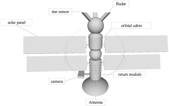
Figure 1.
Three-dimensional structural model of satellite.
Based on the satellite model, a complete three-dimensional point cloud environment was constructed. The point cloud data densely covers multiple module regions and subsidiary structures, while surface normals and obstacle point annotations were incorporated to support spatial traversability analysis and path obstacle-avoidance planning, as shown in Figure 2.
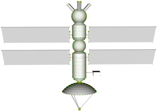
Figure 2.
Point cloud friction coefficient mapping diagram.
It should be noted that the path planning model constructed in this paper does not currently account for non-ideal factors such as sensor noise, actuator errors, and dynamic obstacles. In subsequent research, robust optimization and adaptive replanning strategies will be incorporated to enhance the algorithm’s practical reliability in uncertain environments.
2.2. Workspace Modeling and Configuration Space Transformation
Robot path planning aims to design safe and efficient paths from the starting point to the target. However, the complex obstacles in the physical environment, the robot’s own motion constraints, and the computational complexity of high-dimensional searches pose challenges for precise modeling and real-time solutions. To address this, spatial abstraction and mapping are required to transform the physical workspace into a computable planning space, thereby balancing accuracy and efficiency.
In the three-dimensional workspace , three fundamental sets are defined: the obstacle set , the robot body volume , and the free space accessible to the robot, denoted as
As illustrated in Figure 3, the blue block in the workspace represents the robot entity, whose movement is constrained by the spatial distribution of the red polygonal obstacles. Due to the robot’s physical volume, its actual navigable area in three-dimensional space is smaller than the free space covered by the ideal point-based target path.
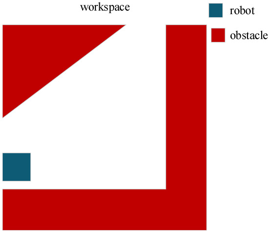
Figure 3.
Path planning workspace.
To address the high complexity of path planning and the difficulty of collision detection in physical spaces, the academic community has introduced the configuration space (C-Space) theory [26]. This method simplifies robots into unstructured particles by expanding obstacles, representing their positions or poses as configuration points.
As shown in Figure 4, the original obstacles together with their inflated boundaries define the configuration space obstacle region . A collision is considered to occur if the robot’s configuration point lies within this region. The inflated obstacles in the configuration space are computed using the Minkowski sum, defined as
where denotes the Minkowski sum, and the inflation radius is determined by the robot’s physical dimensions, the sensing range, and a safety margin, expressed as
where is the effective radius of the robot, accounts for the sensing range, and represents the additional safety margin.
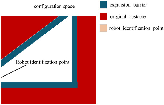
Figure 4.
Path planning configuration space.
In the configuration space, the current position of the robot is represented by its configuration point . If this point does not belong to the obstacle region , the robot is considered to be located in the free space, which is defined as
In the configuration space, the robot is represented by a massless point with no volume and shape. The original obstacles together with the inflated obstacles constitute the configuration space obstacles. Consequently, the path planning problem is transformed into finding a path in the configuration space from the start point to the goal point .
3. Improved A*-B Spline Hybrid Path Planning Algorithm
3.1. A* Algorithm with Multi-Cost Factor Optimization
To plan initial paths that comply with robotic mobility constraints in complex star chart environments, the traditional A* algorithm has been optimized with multiple cost factors. This algorithm no longer relies solely on Euclidean distance as the path cost. Instead, it constructs a comprehensive cost function that integrates path geometric length, surface adhesion safety, traction characteristics, and obstacle avoidance safety. Its core lies in the redefinition of the heuristic function and the actual cost function.
The actual cost represents the accumulated value from the start point to the node . The update formula is given as
where and are the three-dimensional coordinates of nodes and , respectively, and denotes the Euclidean distance. The term is the attraction cost factor, defined as the arithmetic mean of the attraction coefficients of adjacent nodes:
where is the attraction coefficient at a node, reflecting the tribological properties of the surface material and obtained from the predefined friction distribution field . The coefficient ranges within . The greater the attraction coefficient, the larger the weight , and consequently the smaller the actual traversal cost of the corresponding path segment. This design effectively guides the robot to avoid high-friction regions and instead prioritizes traversing areas with lower friction, thereby favoring regions with higher safety.
To ensure that the planned path strictly avoids high-risk obstacles, the algorithm adopts a hard-constrained strategy, explicitly prohibiting the expansion of any node belonging to the high-risk obstacle set . For an expanded neighboring node, the following check is performed:
If node belongs to the high-risk obstacle set, it is skipped directly. This strategy eliminates the risk of collision with high-risk obstacles at the source, thereby constituting the core safeguard for ensuring path safety.
The heuristic cost function estimates the cost from the current node to the goal node , which is computed using the three-dimensional Euclidean distance:
where and are the coordinates of nodes and , respectively. The total cost of node is the sum of the actual cost and the heuristic cost, which serves as the priority ranking criterion in the open list:
where denotes the accumulated path cost from the start node to the current node ; is the heuristic function from to the goal node , representing the estimated cost; and is a weighting parameter. Nodes are expanded in ascending order of . The search proceeds iteratively until the goal is reached or no feasible path exists.
3.2. Cubic B-Spline Optimization Based on Secure Embedding
Smooth path planning typically employs parametric curve methods, commonly including PH curves, Bézier curves, and B-spline curves. Each curve possesses distinct suitability characteristics. Among these methods, this paper selects B-splines as the basis function for trajectory generation, primarily based on their three key advantages in robotic motion planning. The local support property of B-splines allows adjusting individual control points to affect only the local curve segment, facilitating online trajectory correction and real-time replanning. All derivatives of B-splines retain the B-spline form, and control points can be derived through linear relationships, simplifying the imposition of constraints on higher-order motion quantities. Additionally, the convexity of the curve ensures it lies within the convex hull formed by the control point polygon, aiding collision detection and enhancing path safety.
Therefore, to address issues such as the initial path generated by the A* algorithm being composed of discrete points and exhibiting sharp turns, this section employs a cubic uniform B-spline curve with C2 continuity to perform smoothing optimization. This curve not only ensures continuity in both velocity and acceleration along the robot’s motion trajectory but also incorporates a real-time collision detection mechanism to guarantee the absolute safety of the smoothed path.
The mathematical definition of an order B-spline curve is given as
where denotes the coordinates of the control point (a total of control points), and represents the order B-spline basis function. The basis function is computed as
Here, denotes the binomial coefficient.
For the special case of cubic B-spline (), the basis functions can be compactly expressed in matrix form:
Accordingly, the cubic B-spline curve is given by:
When the parameter takes values in the interval , the curve yields the position of each point on a segment. Let and represent the horizontal and vertical coordinates of the curve segment, respectively. They can be expressed as
Traditional B-spline smoothing may result in curve segments deviating from control point envelopes, potentially leading to collisions with obstacles. To address this issue, real obstacle detection is incorporated into the B-spline sampling process, ensuring that each generated path point undergoes safety verification.
Let the high-risk obstacle point cloud set be defined as , where represents the high-risk obstacle set. For each candidate path point , the minimum Euclidean distance to the obstacle set is computed as
With a predefined safety distance threshold , the safety condition can be expressed as
Finally, the smoothed path is constructed by the set of sampled points that satisfy the safety constraint:
3.3. Hybrid Algorithm Collaborative Framework
The improved A* search and B-spline optimization demonstrate significant advantages in global feasibility and local continuity for path planning, respectively. To achieve path generation that balances safety, smoothness, and cost-optimality in complex celestial environments, these two methods are organically integrated. The overall workflow, illustrated in Figure 5, is executed in three phases: map preprocessing, path planning, and curve optimization. First, during map preprocessing, the system generates a sparse 3D mesh map based on point cloud models and annotates terrain elevation, friction coefficients, and obstacle distributions with encoded labels. Subsequently, path search is performed in the constructed graph space using the A* algorithm. Guided by a heuristic function and adjusted by a friction cost term in the cost function, a discrete sequence of path points is generated from the start to the target point. This path satisfies collision-free constraints but may still exhibit structural issues such as abrupt curvature changes or motion discontinuities. In the third stage, the system sparsifies the path and selects key path nodes as control points for input to the B-spline optimization module. Leveraging its high-order continuity, the B-spline curve generates a smooth trajectory between control points, ensuring positional continuity and first-order derivative continuity. This eliminates velocity discontinuities caused by path angularity, enhancing path executability. The final output path undergoes verification against the following characteristics: total path length, maximum curvature, minimum obstacle distance, and average friction cost. This ensures the path meets fundamental requirements for spatial robot task execution in terms of reachability, safety, and physical plausibility.
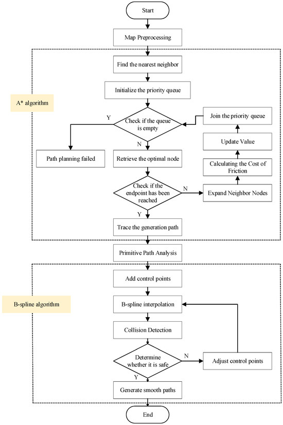
Figure 5.
The overall process of path planning.
4. Voxelized Obstacle Recognition and Friction-Aware Perception
4.1. Voxel-Based Obstacle Detection
Voxelization is a method of discretizing continuous space, which maps a three-dimensional point cloud into fixed-size cubic voxels [27]. Each voxel can be regarded as a unit cube. If a point falls within a voxel, the voxel is considered “occupied.” By setting the voxel size , the target model point cloud can be discretized into voxel indices for subsequent voxel-based comparison. The voxelization process is expressed as
where denotes the voxel side length in meters, representing the voxel resolution.
After the voxel indexing is established, the system first constructs a static reference model point cloud to build the voxel dictionary . This dictionary records all voxel indices occupied by the reference model, serving as the baseline spatial occupancy of the safe region. When the system subsequently acquires the target model point cloud , each point is projected into the voxel space, and its voxel index is compared against the reference dictionary.
If , the point is identified as a new obstacle voxel. The collection of all such points forms the obstacle voxel set:
This approach enables automatic obstacle detection and modeling by comparing voxel indices, even in the absence of explicit geometric reconstruction of the obstacles.
As shown in Figure 6 and Figure 7, the red point set represents the newly detected obstacle points based on the aforementioned voxel difference detection method, which are widely distributed in key areas such as structural edges, external protrusions, and attachment devices.
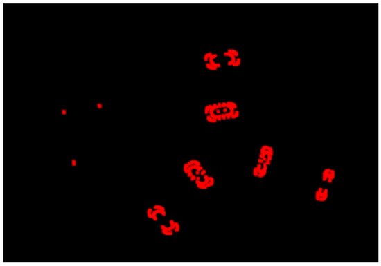
Figure 6.
Schematic diagram of high obstacle recognition results.
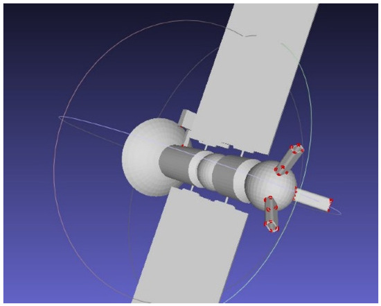
Figure 7.
Visualization of high obstacle recognition results.
4.2. Surface Friction Modeling and Visualization
To more effectively represent surface friction variations on lunar terrain during path planning modeling and enhance quantitative perception of terrain passability, this section proposes a friction coefficient field generation method integrating random perturbations with spatial continuity constraints. A color mapping mechanism is introduced to visualize friction distribution characteristics, aiding in the identification of high-risk areas and the optimization of detour path planning.
In the friction field modeling, each sampled point in the point cloud is first assigned a random value following a uniform distribution using the Monte Carlo method:
This range is based on empirical measurements of typical satellite surface materials. The lower bound of 0.2 represents low-friction regions, while the upper bound of 1.0 corresponds to rough structural surfaces.
To mitigate the variation of friction values caused by randomness, a neighborhood smoothing constraint is introduced for each point , ensuring local consistency of friction coefficients. The constraint is defined as
where denotes the set of the 20 nearest neighboring points of . Experimental verification confirms that this neighborhood smoothing effectively reduces abrupt fluctuations while preserving local detail.
After determining the friction coefficient, RGB mapping rules are further applied to visualize the results. To facilitate intuitive identification of differences in passability across paths, the following linear color coding is employed:
This linear mapping renders higher friction values in shades of green, indicating enhanced passability; conversely, reddish hues denote low friction coefficients, slip hazards, or mechanical adhesion difficulties, signifying hazardous zones. The correspondence between typical friction coefficients and color semantics is shown in Table 1.

Table 1.
Semantic color specification table.
In addition, to enable automated point cloud rendering, high-friction points and regular points are further distinguished through color mapping. The friction coefficient perturbation is defined as
where denotes a random variable uniformly sampled from the interval . This perturbation is mapped into the RGB color space as
As illustrated in Figure 8, the color-coded friction coefficients present a smooth gradient from red to green. The red region corresponds to high-friction areas, the green region represents low-friction areas, and the gradient between them reflects the actual distribution of friction values. This color-coding mechanism enhances the intuitive perception of traversability in path planning and provides visual assistance for subsequent path evaluation and dynamic replanning.
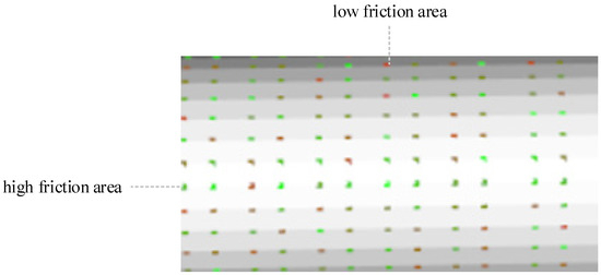
Figure 8.
Point cloud friction coefficient mapping diagram.
Currently, our model treats surface adsorption forces as static constraints based on material properties. However, we clearly recognize that the adsorption force fluctuates dynamically as the robot moves on the surface, which is a process involving complex contact mechanics. Therefore, in this phase of the study focusing on geometric path planning, we do not address this dynamic effect for the time being, and the problem will be addressed in future high-fidelity simulations and physical verification.
5. Optimization Problems and Solutions
The path planning problem can essentially be regarded as a multi-objective optimization problem, in which an evaluation function is typically constructed to quantitatively assess the quality of different candidate paths. For the three-dimensional path planning problem of a space robot operating in an asteroid environment, the proposed comprehensive evaluation function consists of three components: path length, path smoothness, and obstacle avoidance capability. The formulation is given as
where denotes the overall evaluation function, represents the path length evaluation function, is the path smoothness evaluation function, and is the obstacle avoidance evaluation function. The coefficients , , are the weighting factors corresponding to each evaluation function.
For the path length metric , the evaluation is based on the total distance traveled from the start point to the goal point. Given a path represented by a directed graph consisting of a set of edges, it can be expressed as
and the path length evaluation function can be expressed as the cumulative sum of edge lengths:
The path smoothness metric reflects the continuity of the path and the variation of curvature. For a continuous path , the curvature radius and heading variation are incorporated to define the weighted smoothness function as
where denotes the curvature radius at path point , and represents the heading change rate, capturing the oscillatory behavior of curvature variations along the path.
For different types of robots and application scenarios, the weighting coefficients and can be adjusted accordingly. In general, the stronger the robot’s turning capability, the lower the requirement for path smoothness, and thus the smaller the smoothness weighting coefficient . For a given robot configuration, the smaller the ratio , the smoother the optimal path tends to be. For robots with rigid structures, smoothness stability is of critical importance, and therefore the coefficient should be assigned a relatively larger value.
For the obstacle distance evaluation function , during the trajectory planning process, in addition to avoiding direct collisions with obstacles, it is also necessary to provide sufficient clearance for sensors and other peripheral components. This requires that the minimum distance between the trajectory and surrounding obstacles remains sufficiently large. For a given path , let denote the minimum distance between the path point and its nearest obstacle. The obstacle distance evaluation function is then defined as
Here, is formulated as the sum of the reciprocals of the minimum distances from all path points to obstacles. This design effectively penalizes trajectories that pass too close to obstacles, while paths maintaining larger clearance are less affected, thereby ensuring that path optimization accounts for safety in addition to length and smoothness.
In practical path planning, the weighting coefficients , , can be flexibly adjusted according to mission requirements, balancing the relative importance of path length, smoothness, and safety. The final optimization objective is expressed as
6. Simulation Experiment
6.1. Experimental Platform and Scenario Construction
To validate the practicality and performance of the proposed A*-B spline path planning algorithm under varying surface conditions and structural complexities, this paper establishes a standardized testing platform. The algorithm’s core components were developed using C++17 within the Visual Studio 2022 development environment. The hardware platform consists of a Lenovo Y7000P laptop equipped with an Intel i7-9750H CPU and NVIDIA GTX 1660 Ti GPU, providing sufficient computational power for 3D point cloud processing and real-time path generation.
6.2. Path Generation and Comparative Analysis
This section systematically compares the A* algorithm with the improved A*-B spline hybrid algorithm based on 12 typical path planning cases and dataset results. The experiments utilize a high-precision satellite 3D model incorporating typical components such as parabolic antennas and solar panel arrays. The model surface is constructed into a point cloud map through ordered sampling with a density of 200 pts/m2. The frame rate was stabilized at 33.3 FPS, meeting real-time planning requirements. Figure 9 displays the visualization results of 12 path planning case studies.
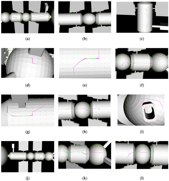
Figure 9.
12 sets of path planning visualization results. (a–l) respectively display the path planning results of the A* algorithm (purple) and the A*-B-spline hybrid algorithm (green) across 12 experimental groups. The figures demonstrate that the A*-B-spline paths maintain shorter path lengths while significantly enhancing path smoothness and continuity, particularly excelling in complex surfaces and densely obstructed areas.
Table 2 lists the 12 experimental datasets employed in this study, designed primarily based on the following aspects: Regarding environmental characteristics, experiments cover various typical 3D scenarios including “cross-sectional environments,” “transition zones,” and “complex surfaces” to systematically evaluate algorithm performance in both structured and unstructured environments. In terms of path types, datasets are categorized into hierarchical levels including “global planning,” “mid-range planning,” and “local obstacle avoidance,” reflecting multi-level planning requirements from macro-level path generation to local dynamic adjustments. In terms of scenario specificity: Sets 1 and 10 test algorithm stability under long-distance, full-dimensional variations; Sets 6, 7, and 9 focus on verifying obstacle avoidance capabilities; Sets 3 and 4 target vertical motion and complex surface scenarios, evaluating algorithm performance under elevation changes and multi-constraint conditions. Furthermore, all start and end coordinates are defined within the simulated environment, encompassing spatial distribution patterns such as horizontal expansion, vertical variation, and diagonal movement. This ensures the representativeness and reproducibility of experimental data, establishing a systematic baseline for subsequent performance evaluations in the figure.
Table 2.
12 sets of experimental data sets.
Next, a quantitative comparison and analysis was conducted on the differences in path planning effects between the A* algorithm and the A*-B spline hybrid algorithm. The analysis focused on two dimensions: geometric features and motion features. All the relevant analyses were based on the 12 sets of origin-destination path experimental data mentioned above.
6.2.1. Geometric Feature Analysis
A quantitative analysis of twelve path planning samples shows that the improved A*-B-spline hybrid algorithm outperforms the traditional A* algorithm in path geometry. In terms of path length, the hybrid algorithm achieves an average reduction of 6.82%. In Experiment 3, the length dropped from 57.41 m to 51.36 m, an improvement of 10.54%. This reduction results mainly from the B-spline smoothing process, which removes redundant turning points and reduces path backtracking.
Path smoothness shows even greater improvement. The maximum directional change angle decreased sharply from 90.1° ± 3.7° to 11.0° ± 1.1°, a reduction of 87.8%. All sharp turns were eliminated. The number of sharp turns fell from 8.3 to 0, representing a 100% optimization rate. These results confirm that the B-spline algorithm effectively removes the abrupt corners produced by the A* algorithm, yielding smooth paths that satisfy robotic kinematic constraints. The detailed data are presented in Table 3. The arrows in the Improvement-Rate column indicate the direction of change: ↓ denotes a decrease and ↑ denotes an increase.
Table 3.
Comparison of geometric features between A* algorithm and improved A*-B spline algorithm (mean ± standard deviation).
6.2.2. Energy Consumption and Execution Time Analysis
The average energy consumption of the hybrid algorithm was 469.80 ± 329.10, an increase compared to the 165.19 ± 109.83 recorded for Algorithm A. In terms of execution time, the hybrid algorithm averaged 206.83 ± 128.45 ms, also higher than the 84.17 ± 53.51 ms achieved by Algorithm A. Nevertheless, it should be noted that the proposed method completes trajectory planning within milliseconds on standard personal computer platforms, demonstrating its potential for real-time applications. This result indicates that the computational resources invested in the A*-B-spline algorithm primarily translate into a significant improvement in path quality. For satellite robots, the combined benefits of reduced path length—including energy savings, protection of mechanical structures from abrupt turns, and enhanced control precision through smoother paths—far outweigh the additional computational overhead. Particularly in long-term orbital missions, minimizing mechanical wear and enhancing mobility reliability take precedence over computational time. Future work will involve porting this algorithm to representative embedded systems and conducting benchmark testing to further validate its performance in real-world deployment scenarios.
6.2.3. Kinematic Characteristics and Safety Performance Analysis
Regarding path curvature metrics, the hybrid algorithm achieved an average curvature of 0.1358 m−1, slightly lower than the A* algorithm’s 0.1365 m−1, indicating a marginal improvement in overall path smoothness. However, its maximum curvature mean increased from 0.66 m−1 to 1.20 m−1, representing an approximately 82% rise. This primarily stems from the introduction of small-radius segments in local regions by B-spline curves to achieve greater smoothness and continuity. On the other hand, the overall uniformity of curvature distribution showed no significant difference, with variance decreasing only slightly from 7.66 × 10⁻⁴ to 7.30 × 10⁻⁴—a reduction of about 4.6%—indicating that curvature fluctuations remained generally stable. Regarding directional continuity, the hybrid algorithm continues to demonstrate advantages, particularly in mitigating abrupt changes during high-angle turns, resulting in smoother path transitions.
In Group 1 long-distance path planning(where the purple path represents the A* algorithm and the green path represents the A*-B-spline algorithm), the path lengths for the A* algorithm and hybrid algorithm were 324.9m and 304.4m, respectively, representing a reduction of approximately 6.33%. Simultaneously, all sharp turns were completely eliminated, reducing their number from 28 to 0, and the maximum direction change angle was optimized from 92.0° to 10.5°, demonstrating superior path smoothness, as shown in the detailed section of Figure 10. Regarding path dynamics cost, the hybrid path avoids unnecessary sharp turns and backtracking maneuvers, resulting in increased theoretical energy consumption. This indicates superior motion economy and execution feasibility for long-distance paths.
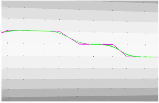
Figure 10.
Group 1 local detail diagrams.
In the typical obstacle avoidance task of Group 7, the hybrid path actively adjusts the path curvature radius and control point layout through spline configuration, achieving efficient navigation around local obstacle clusters. As shown in Figure 11, all high-density obstacle zones were avoided without sacrificing path length, and no path-obstacle overlap nodes occurred, further validating the algorithm’s dynamic adaptability in local obstacle environments.
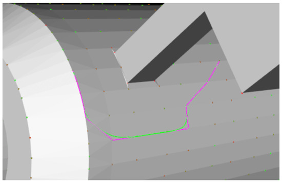
Figure 11.
Group 7 detail images.
The statistical results for Group 10 reveal that the original A* path contained as many as 32 sharp turns with directional change angles exceeding 60°. After B-spline smoothing, such abrupt changes were completely eliminated, resulting in highly continuous steering transitions, as shown in Figure 12. Furthermore, the maximum directional change angle along the path decreased from 93.7245° to 12.0414°, clearly demonstrating the hybrid algorithm’s superior robustness and controllability in terms of feasibility.
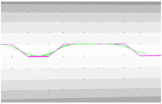
Figure 12.
Group 10 local detail diagrams.
Overall, the A*-B-spline path effectively mitigates issues like path discontinuity and abrupt turns at the kinematic level, enhancing path tracking stability and robotic driving comfort. From a safety perspective, regarding obstacle avoidance capability, the minimum safety distance between paths generated by the hybrid algorithm and obstacles increased from 21.47 to 21.83m, representing a 1.67% improvement. This effectively expands the obstacle avoidance margin of the path and reduces potential collision risks.
6.3. Multi-Algorithm Comparison Experiment
To further validate the comprehensive performance of the A*-B-spline hybrid algorithm in complex satellite surface path planning, this section introduces the Rapidly-exploring Random Tree (RRT) algorithm based on random sampling as a comparative benchmark, establishing a framework for comparing the three algorithms. The experiment is conducted in a typical satellite surface transition zone, with the starting coordinates at (97.25, 61.3099, 234.87) and the ending coordinates at (157.199, 43.4477, 237.158). This region incorporates typical features such as surface transitions and localized obstacle distributions, effectively testing the geometric adaptability and motion continuity performance of each algorithm. The path planning results for the three algorithms are shown in Figure 13, where purple represents the traditional A* algorithm, green represents the A*-B-spline hybrid algorithm, and cyan represents the RRT surface path planning algorithm. A quantitative comparison of the key performance metrics for the three algorithms is presented in Table 4.
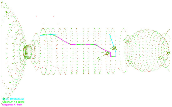
Figure 13.
Result diagram of the three algorithms path planning.
Table 4.
Comparison of geometric features among three algorithms (mean ± standard deviation).
From the analysis of path geometric characteristics, the A*–B-spline hybrid algorithm demonstrated optimal performance in path length at 64.78 m. This represents a 5.64% reduction compared to the A* algorithm’s 68.65 m and a 14.95% reduction compared to the RRT algorithm’s 76.17 m. This advantage primarily stems from the B-spline curve’s optimization of redundant turning points along the path, achieving path length compression through the redistribution of control points. In terms of path smoothness, the A-B spline algorithm demonstrated overwhelming superiority, successfully reducing the maximum directional change angle from 90° for the A algorithm and 75.37° for the RRT algorithm to 9.23°, representing reductions of 89.74% and 87.75%, respectively. Simultaneously, the algorithm completely eliminates sharp turns in the path, reducing their number from 2 in A* and 1 in RRT to 0, demonstrating the significant effect of B-spline smoothing on improving path continuity.
Regarding curvature characteristics, the three algorithms exhibit distinct distribution patterns. The RRT algorithm, employing a random sampling strategy, naturally produces paths with superior curvature uniformity. Its average curvature is 0.031 m−1, maximum curvature is 0.091 m−1, both the lowest among the three algorithms, and its curvature variance is only 0.0013, indicating the smoothest path curvature. The A*–B-spline algorithm outperformed the A* algorithm in average curvature, achieving a 21.51% improvement. This demonstrates the role of spline curves in overall path smoothing. However, in local regions, to maintain higher-order continuity, the B-spline curve incorporates segments with smaller radii, resulting in a maximum curvature of 0.595 m−1. This exceeds both the A* algorithm’s 0.408 m−1 and the RRT algorithm’s 0.091 m−1. This phenomenon reflects the trade-off between smoothness and curvature extremes in path planning.
Regarding path quality metrics, the A*-B-Spline algorithm achieved a total cost of 211.732, surpassing the A* algorithm’s 82.955 and the RRT algorithm’s 81.729. This higher value primarily stems from the B-spline curve’s comprehensive optimization of multiple objective functions, including path length, curvature continuity, and safety. Regarding safety, the RRT algorithm achieved the maximum minimum safe distance due to its random expansion feature, demonstrating superior obstacle avoidance robustness. The A algorithm and A-B spline algorithm yielded similar safe distances of 6.495 m and 6.428 m, respectively. Though lower than RRT, these values still meet the basic safety requirements for satellite path planning. In computational efficiency, Algorithm A demonstrated optimal performance, completing in just 37 milliseconds. The A*-B spline algorithm, incorporating an additional B-spline optimization step, increased execution time to 73 milliseconds. The RRT algorithm’s computational time was significantly higher than both Algorithm A and the A*-B spline algorithm. These results clearly reveal the trade-offs among different algorithms in path planning: While the A* algorithm offers a distinct advantage in computational efficiency, the paths it generates exhibit noticeable jaggedness and abrupt directional changes, making them unsuitable for robots requiring smooth motion. The RRT algorithm produces more natural paths but at the cost of significantly increased path length, leading to reduced motion efficiency. In contrast, the A*-B-Spline hybrid algorithm maintains the advantage of path length while completely eliminating abrupt directional changes through B-spline smoothing. It generates continuous trajectories compliant with robotic kinematic constraints. Although computational time increases, the enhanced path quality is crucial for ensuring stable operation of the planetary robot, fully demonstrating the algorithm’s comprehensive advantages in complex surface path planning.
Although this paper focuses on the optimization of geometric paths, the generated B-spline curves are highly suitable as front-end solutions for subsequent dynamic trajectory optimization due to their excellent properties of higher-order continuity. In future work, it will be straightforward to generate dynamically feasible trajectories by introducing constraints such as velocity, acceleration, and jerk and by performing time parameterization based on the geometric paths generated by this algorithm.
7. Conclusions
To address path planning challenges for space robots navigating complex satellite surfaces, this study proposes an innovative hybrid A*-B-spline algorithm. Through system simulation verification in typical satellite surface environments, the algorithm demonstrates significant performance advantages: Compared to traditional A* algorithms and methods like RRT, the new approach not only generates smoother, continuous trajectories that satisfy kinematic constraints but also effectively avoids surface protrusions in complex terrain. It prioritizes traversing high-friction areas to enhance movement stability. Both quantitative and qualitative analyses confirm that the proposed hybrid algorithm successfully achieves synergistic optimization of path geometry and motion continuity. While ensuring safety, it demonstrates superior comprehensive performance in path smoothness, directional continuity, and robustness. To address the current limitations of this work, our future research will advance along three interconnected directions. We will first establish a ground-based physical platform to validate the algorithm’s performance with dynamic experiments in a simulated satellite environment. Subsequently, we will extend the framework to multi-robot collaborative planning, enhancing coordination and execution efficiency in complex scenarios. Ultimately, we will incorporate real-world factors—including sensor noise, variable load conditions, actuator errors, and dynamic obstacles—to bolster the algorithm’s robustness in uncertain environments. The integration of these dynamic constraints will enable the generation of realistic, real-time trajectories from geometric paths, thereby laying a crucial technological foundation for future in-orbit services.
Author Contributions
Conceptualization, X.L. and W.Z.; methodology, X.L.; software, X.L.; validation, X.L., C.Z. and S.G.; formal analysis, X.L.; investigation, X.L.; resources, C.Z.; data curation, X.L.; writing—original draft preparation, X.L.; writing—review and editing, W.Z., C.Z. and S.G.; visualization, X.L.; supervision, W.Z. and Z.X.; project administration, W.Z.; funding acquisition, W.Z. All authors have read and agreed to the published version of the manuscript.
Funding
This research received no external funding.
Data Availability Statement
Data used to support this study are available from the authors upon request.
Conflicts of Interest
The authors declare no conflicts of interest.
References
- Wen, C.; Zheng, P.; Jing, Z.; Guo, C.; Chen, C. Force–Position Coordinated Compliance Control in the Adhesion/Detachment Process of Space Climbing Robot. Aerospace 2024, 12, 20. [Google Scholar] [CrossRef]
- Hawkes, E.W.; Jiang, H.; Cutkosky, M.R. Three-Dimensional Dynamic Surface Grasping with Dry Adhesion. Int. J. Robot. Res. 2016, 35, 943–958. [Google Scholar] [CrossRef]
- Huang, C.; Liu, Y.; Bai, B.; Wang, K. The Flying and Adhesion Robot Based on Approach and Vacuum. Aerospace 2022, 9, 228. [Google Scholar] [CrossRef]
- Zhang, J.; Zhang, J.; Zhang, Q.; Wei, X. Obstacle Avoidance Path Planning of Space Robot Based on Improved Particle Swarm Optimization. Symmetry 2022, 14, 938. [Google Scholar] [CrossRef]
- Katona, K.; Neamah, H.A.; Korondi, P. Obstacle Avoidance and Path Planning Methods for Autonomous Navigation of Mobile Robot. Sensors 2024, 24, 3573. [Google Scholar] [CrossRef]
- Lyu, D.; Chen, Z.; Cai, Z.; Piao, S. Robot Path Planning by Leveraging the Graph-Encoded Floyd Algorithm. Future Gener. Comput. Syst.-Int. J. Esci. 2021, 122, 204–208. [Google Scholar] [CrossRef]
- Yang, Y.; Luo, X.; Li, W.; Liu, C.; Ye, Q.; Liang, P. AAPF*: A Safer Autonomous Vehicle Path Planning Algorithm Based on the Improved A* Algorithm and APF Algorithm. Clust. Comput. 2024, 27, 11393–11406. [Google Scholar] [CrossRef]
- Li, X.; Li, G.; Bian, Z. Research on Autonomous Vehicle Path Planning Algorithm Based on Improved RRT* Algorithm and Artificial Potential Field Method. Sensors 2024, 24, 3899. [Google Scholar] [CrossRef]
- Guan, T.; Han, Y.; Kong, M.; Wang, S.; Feng, D.; Yang, W. An Improved Artificial Potential Field with RRT Star Algorithm for Autonomous Vehicle Path Planning. Sci. Rep. 2025, 15, 16982. [Google Scholar] [CrossRef]
- Zengin, H.A.; Isik, A.H. Improvement for Traditional Genetic Algorithm to Use in Optimized Path Finding. Artif. Intell. Appl. Math. Eng. Probl. 2020, 43, 473–483. [Google Scholar]
- He, C.; Lian, S.; Shi, Q.; Miao, Z. An Improved Joint Space Astar Algorithm for a 6-DOF Manipulator with Pre-Planning Strategy. Sci. Rep. 2025, 15, 18164. [Google Scholar] [CrossRef] [PubMed]
- Tang, L. Research on Path Planning of Lunar Exploration Robot Based on A* Algorithm. IET Conf. Proc. 2024, 2024, 481–486. [Google Scholar] [CrossRef]
- Wang, K.; Peng, S.; Liu, S.; Li, H. Study on Path Planning of Lunar Rover Based on A* Algorithm Optimization. Spacecr. Eng. 2019, 28, 19–26. [Google Scholar]
- Miyombo, M.E.; Liu, Y.; Mulenga, C.M.; Siamulonga, A.; Kabanda, M.C.; Shaba, P.; Xi, C.; Ayodeji, A. Optimal Path Planning in a Real-World Radioactive Environment: A Comparative Study of A-Star and Dijkstra Algorithms. Nucl. Eng. Des. 2024, 420, 113039. [Google Scholar] [CrossRef]
- Chen, Y.; Guo, J.; Yang, H.; Wang, Z.; Liu, H. Research on Navigation of Bidirectional A* Algorithm Based on Ant Colony Algorithm. J. Supercomput. 2021, 77, 1958–1975. [Google Scholar] [CrossRef]
- Fransen, K.; Van Eekelen, J. Efficient Path Planning for Automated Guided Vehicles Using A* (Astar) Algorithm Incorporating Turning Costs in Search Heuristic. Int. J. Prod. Res. 2023, 61, 707–725. [Google Scholar] [CrossRef]
- Zheng, W.; Huang, K.; Wang, C.; Liu, Y.; Ke, Z.; Shen, Q.; Qiu, Z. Research on 3D Path Planning of Quadrotor Based on Improved A* Algorithm. Processes 2023, 11, 334. [Google Scholar] [CrossRef]
- Peng, J.; Huang, Y.; Luo, G. Robot Path Planning Based on Improved A* Algorithm. Cybern. Inf. Technol. 2015, 15, 171–180. [Google Scholar] [CrossRef]
- Bay, T.; Cattiaux-Huillard, I.; Romani, L.; Saini, L. On G1 and G2 Hermite Interpolation by Spatial Algebraic-Trigonometric Pythagorean Hodograph Curves with Polynomial Parametric Speed. Appl. Math. Comput. 2023, 458, 128240. [Google Scholar] [CrossRef]
- Bulut, V. Path Planning for Autonomous Ground Vehicles Based on Quintic Trigonometric Bezier Curve: Path Planning Based on Quintic Trigonometric Bezier Curve. J. Braz. Soc. Mech. Sci. Eng. 2021, 43, 104. [Google Scholar] [CrossRef]
- Sun, Y.; Wang, H. Research on B-Spline Curve Trajectory Planning Method Considering Curvature. In Proceedings of the 2024 8th International Conference on Robotics, Control and Automation, Icrca, Shanghai, China, 12–14 January 2024; pp. 211–216. [Google Scholar]
- Shi, J.; Su, Y.; Bu, C.; Fan, X. A Mobile Robot Path Planning Algorithm Based on Improved A*. J. Phys. Conf. Ser. 2020, 1486, 032018. [Google Scholar] [CrossRef]
- Lai, R.; Wu, Z.; Liu, X.; Zeng, N. Fusion Algorithm of the Improved A* Algorithm and Segmented Bézier Curves for the Path Planning of Mobile Robots. Sustainability 2023, 15, 2483. [Google Scholar] [CrossRef]
- Zhang, Y.; Xue, Q.; Ji, S. Continuous Path Smoothing Method of B-Spline Curve Satisfying Curvature Constraint. J. Huazhong Univ. Sci. Technol. Nat. Sci. 2022, 50, 59–65+72. [Google Scholar]
- Fan, B.; Chen, P. Continuous Path Smoothing for Deep-Sea Mining Vehicles Using B-Spline Curves. Proc. Inst. Mech. Eng. Part D-J. Automob. Eng. 2025, 09544070251315532. [Google Scholar] [CrossRef]
- Liu, Y.; Zhang, X.; Wu, C.; Yang, M. Obstacle Avoidance Planning for Industrial Robots Based on Singular Manifold Splitting Configuration Space. Concurr. Comput.-Pract. Exp. 2024, 36, e8245. [Google Scholar] [CrossRef]
- Gonizzi Barsanti, S.; Marini, M.R.; Malatesta, S.G.; Rossi, A. Evaluation of Denoising and Voxelization Algorithms on 3D Point Clouds. Remote Sens. 2024, 16, 2632. [Google Scholar] [CrossRef]


Disclaimer/Publisher’s Note: The statements, opinions and data contained in all publications are solely those of the individual author(s) and contributor(s) and not of MDPI and/or the editor(s). MDPI and/or the editor(s) disclaim responsibility for any injury to people or property resulting from any ideas, methods, instructions or products referred to in the content. |
© 2025 by the authors. Licensee MDPI, Basel, Switzerland. This article is an open access article distributed under the terms and conditions of the Creative Commons Attribution (CC BY) license (https://creativecommons.org/licenses/by/4.0/).