A Combined Optimization Method for the Transition Control Schedules of Aero-Engines

Abstract

A well designed transition control schedule can enable the engine to quickly and smoothly transition from one operating state to another, thereby enhancing the maneuverability of the aircraft. Although traditional pointwise optimization methods are fast in solving the transition control schedules, their optimized control schedules suffer from fluctuation problems. While global optimization methods can suppress fluctuation problems, their slow solving speed makes them unsuitable for engineering applications. In this paper, a combined optimization method for the transition control schedules of aero-engines is proposed. This method divided the optimization of the control schedules into two layers. In the outer-layer optimization, the global optimization technique was utilized to suppress the fluctuation of geometrically adjustable parameters. In the inner-layer optimization, the pointwise optimization technique was adopted to quickly obtain the control schedule of fuel flow rate. Moreover, a construction method of non-uniform control points in the global optimization layer was proposed, which significantly reduced the number of control points that needed to be optimized; thus, improving the efficiency of global optimization. The optimization problem of the acceleration and deceleration control schedules of a mixed-flow turbofan engine was used to verify the effectiveness of the combined optimization method. The results show that, compared with the pointwise optimization method, the transition time optimized by the combined optimization method shows no obvious difference. The control schedules optimized by the combined optimization method are not only smooth but can also prevent some components from approaching their working boundaries.

1. Introduction

The transition performance of aero-engines plays a crucial role in aircraft maneuverability. However, due to the complexity and strong nonlinearity of aero-engines, it is difficult to quickly design the optimal transition control schedules within the constraints [1,2]. At present, there are mainly two types of optimization methods for the transition control schedules of aero-engines, which are the pointwise optimization methods and the global optimization methods.

The pointwise optimization methods discretize the optimization problem of the transition control schedules into sub-optimization problems at each time step or discrete operating point. These methods attempt to adjust the engine’s adjustable parameters within each sub-optimization problem, enabling the engine to complete the transition operation rapidly and smoothly. Hao [3] and Zheng [4] ignored the engine’s dynamic effects and optimized the adjustable parameters of key working points in the transition process based on the engine’s steady-state model. Although a smooth mode transition of the variable cycle engine was achieved, the neglect of dynamic effects led to low design accuracy of the transition control schedules and an inability to guarantee the minimum mode transition time. Chen [5,6,7] and Kurzke [8] proposed the virtual power extraction method that can use the power extraction for the steady state of the engine to simulate the remaining power in the transition process. Thus, the transition control schedules of the engine can be analyzed and optimized at discrete steady-state operating points. Jia [9,10,11] proposed a transition process reverse method based on the virtual power extraction method. This method incorporates specific adjustable parameters and performance parameters of the engine into the unknown variables and equilibrium variables of the equations for the engine model, respectively. During the process of solving the engine equations, the adjustable parameters corresponding to the specified performance parameters can be automatically solved; thus, simplifying the design process of the transition control schedules. However, the virtual power extraction method assumes that the relationship between the rotational speeds of the high-pressure and low-pressure rotors in the transition process is the same as that in the steady state. Moreover, it ignores dynamic factors such as the volume effect, resulting in a low design accuracy of the transition control schedules. Lu et al. [12] iterated the virtual power extraction method and used the optimized transition control schedules from the previous step to calculate the relationship between the rotational speeds of the high-pressure and low-pressure rotors. Although this has improved the optimization accuracy, it has also multiplied the optimization time. Qi [13] and Li [14] proposed a kind of pointwise optimization method that directly optimizes the adjustable parameters of the engine at each time step during the transition process, and obtained the control schedule curves of fuel flow rate and nozzle throat area during the acceleration process. The pointwise optimization methods are widely used for various aero-engines due to their relatively fast optimization speed [15,16,17,18,19]. However, since they do not consider the relationship between working points in the transition process, there are fluctuations in the optimized control schedules [20]. Zhao et al. [21] constrained the adjustable parameters at the current time step according to the predicted values of the performance parameters in the next few time steps. Although this suppresses the high-frequency fluctuations of the control schedules, it prolongs the transition time. Hao [22,23] and Zhang [24] added constraints on the change rate of adjustable parameters in pointwise optimization, largely inhibiting the high-frequency fluctuations of control schedules. However, there are still low-frequency fluctuations. To suppress the fluctuation problem that occurs in the pointwise optimization methods, the global optimization methods are proposed.

The global optimization methods parameterize the transition control schedule curves into discrete control points. These methods directly optimize the control points to minimize the transition time. Moreover, it is quite easy to enhance the smoothness of the control curves by various means. Zhang et al. [25] restricted the control parameters to change monotonically during the global optimization. While this enhanced the smoothness of the control schedules, it significantly limited the flexibility of the control schedules, thus, making it impossible to guarantee the shortest transition time. Zheng et al. [20]. used Bezier curves to construct the control schedules for fuel flow rate and nozzle throat area and directly optimized the control points of the Bezier curve to minimize the acceleration time. The smoothness of the Bezier curve effectively suppresses the fluctuation problem of the control schedules. Song et al. [26] introduced the maximum entropy theory in the global optimization method. They suppressed the high-frequency fluctuations by maximizing the entropy value of the control schedules. Additionally, they suppressed the low-frequency fluctuations through the piecewise linearization of the optimized control schedules. Although the global optimization methods demonstrate advantages in suppressing fluctuations of control schedules, they involve numerous control points of the control schedules, which leads to a high-dimensional global optimization problem. Moreover, repeated evaluations of transition times for different control schedules make the optimization time cost unacceptable. To reduce the time for global optimization, Ye et al. [27,28,29] used surrogate models to estimate the engine’s transition time. However, due to the complexity of the aero-engines, it is difficult to guarantee the accuracy of surrogate models, which leads to noticeable differences in the control schedules and transition times obtained from different surrogate models.

In this paper, a combined optimization method for the transition control schedules of aero-engines is proposed. This method divides the optimization of control schedules into two layers. For the inner-layer optimization, the pointwise optimization technique is used to quickly optimize the control schedules that usually do not fluctuate. For the outer-layer optimization, the global optimization technique is employed to suppress the control schedules that are prone to fluctuations. Furthermore, to reduce the time cost of global optimization, a construction method of non-uniformly distributed control points is proposed. Thus, the number of control points that need to be optimized can be reduced.

The rest of this paper is organized as follows. Section 2 introduces the transition optimization problem of engines. Section 3 elaborates on the principle, process, and innovation of the combined optimization method. In Section 4, the method is applied to the optimization of acceleration and deceleration control schedules for a mixed-flow turbofan engine to verify its effectiveness and advancement. Section 5 presents a summary of this paper.

2. Transition Optimization Problem of Aero-Engines

2.1. The Mathematical Formulation of the Transition Optimization Problem

The transition process of aero-engines mainly includes acceleration and deceleration processes. The acceleration process refers to pushing the power lever to make the engine transition from a low-thrust state to a high-thrust state. The deceleration process is the opposite. The transition time of an aero-engine is its key dynamic performance. When the power lever is pushed rapidly for acceleration, the fuel flow rate increases swiftly, followed by a rise in the outlet temperature of the combustor and the rotor speed. In addition, the operating point of the compressor will move towards its surge boundary, as shown in Figure 1. During the acceleration process, the compressor should maintain a sufficient surge margin to ensure that its working point does not approach the surge boundary too closely. During the deceleration process, there is no need to worry about the operating point of the compressor becoming too close to the surge boundary. However, it is necessary to limit the minimum value of the fuel flow rate to prevent the combustor from flame-out. Therefore, in the transition process, it is not only required to have a short transition time but also necessary to ensure the reliable operation of the engine. Typically, in the transition process, it is required that parameters such as the compressor surge margin, rotor speed, and combustor outlet temperature do not exceed the limit values.

Generally, the transition control schedules for the engine can be expressed as the relationship between adjustable parameters and time:

$$\mathit{X}(t)=[x_1(t),x_2(t),\cdot \cdot \cdot ,x_i(t),\cdot \cdot \cdot ,x_I(t)]$$

(1)

where $x_i(t)$ represents the value of the i-th adjustable parameter at time t and I represents the number of adjustable parameters.

The control schedule curves of adjustable parameters during the transition process can be optimized, so that the engine can complete the transition process quickly and reliably. The objective function of the transition process optimization can be expressed as the following:

$$\left\{\begin{array}{l}\min \hspace{0.33em}O={\displaystyle \underset{0}{\overset{t}{\int }}{\left(P(\mathit{X}(t))-P_{\mathrm{target}}\right)}^2}dt\\ s.t.\hspace{0.33em}{g}_j(\mathit{X}(t))\le 0, j=1,2,3\dots J\end{array}\right.$$

(2)

where $\mathit{P}$ represents the performance parameter of the engine, which is usually the thrust or rotor speed (in this paper, the thrust is selected as $\mathit{P}$); $P_{\mathrm{target}}$ represents the target value of the performance parameter at the end of the transition process; $g_j$ denotes the j-th constraint condition during the transition process; and $J$ represents the number of constraint conditions.

For the mixed-flow turbofan engine studied in this paper, the constraint conditions to be met during the transition process are shown below:

$$\left\{\begin{array}{l}{g}_1(\mathit{X}(t))={\displaystyle \frac{{\mathrm{SM}}_{\mathrm{F},\min }-{\mathrm{SM}}_{\mathrm{F}}(\mathit{X}(t))}{{\mathrm{SM}}_{\mathrm{F},\min }}}\\ g_2(\mathit{X}(t))={\displaystyle \frac{{\mathrm{SM}}_{\mathrm{C},\min }-{\mathrm{SM}}_{\mathrm{C}}(\mathit{X}(t))}{{\mathrm{SM}}_{\mathrm{C},\min }}}\\ g_3(\mathit{X}(t))={\displaystyle \frac{N_{\mathrm{L}}(\mathit{X}(t))-N_{\mathrm{L},\max }}{N_{\mathrm{L},\max }}}\\ g_4(\mathit{X}(t))={\displaystyle \frac{N_{\mathrm{H}}(\mathit{X}(t))-N_{\mathrm{H},\max }}{N_{\mathrm{H},\max }}}\\ g_5(\mathit{X}(t))={\displaystyle \frac{T_4(\mathit{X}(t))-T_{4,\max }}{T_{4,\max }}}\\ g_6(\mathit{X}(t))={\displaystyle \frac{M{a}_{22}(\mathit{X}(t))-M{a}_{22,\max }}{M{a}_{22,\max }}}\\ g_7(\mathit{X}(t))={\displaystyle \frac{\dot{\mathit{X}}(t)-{\dot{\mathit{X}}}_{\max }}{{\dot{\mathit{X}}}_{\max }}}\end{array}\right.$$

(3)

where the subscripts min and max, respectively, represent the lower and the upper limits of the parameter; ${\mathrm{SM}}_{\mathrm{F}}$ and ${\mathrm{SM}}_{\mathrm{C}}$ respectively represent the surge margins of the fan and the high-pressure compressor; $N_{\mathrm{L}}$ and $N_{\mathrm{H}}$ respectively represent the rotational speeds of the low-pressure rotor and the high-pressure rotor; $T_4$ represents the combustor outlet temperature; $M{a}_{22}$ represents the Mach number at the outlet of the fan bypass duct; $\dot{\mathit{X}}$ represents the change rate of the adjustable parameters.

2.2. Traditional Optimization Methods for Transition Control Schedules

Traditional optimization methods for transient control schedules mainly include the pointwise optimization methods and the global optimization methods.

The pointwise optimization methods discretize the objective function described by Equation (2) into each time step of the transition process:

$$\left\{\begin{array}{l}\min \hspace{0.33em}O(t_k)={\left(P(\mathit{X}(t_k))-P_{\mathrm{target}}\right)}^2\\ s.t.\hspace{0.33em}\hspace{0.33em}\hspace{0.17em}{g}_j(\mathit{X}(t_k))\le 0,\hspace{0.33em}j=1,2,3\dots J\end{array}\right.$$

(4)

where $O(t_k)$ represents the objective function of the k-th time step and $\mathit{X}(t_k)$ represents the adjustable parameters at the end of the k-th time step.

At each time step during the transition process, the $\mathit{X}(t_k)$ is optimized to satisfy Equation (4), so that the performance parameter of the engine can quickly approach its target value. For engines with multiple adjustable parameters, Equation (4) needs to be further expanded as follows:

$$\left\{\begin{array}{l}\min \hspace{0.33em}O(t_k)={\left({\displaystyle \frac{P(\mathit{X}(t_k))-P_{\mathrm{target}}}{P_{\mathrm{target}}-P_{\mathrm{start}}}}\right)}^2\left(1-\omega \right)+\omega {\displaystyle {\sum }_{i=1}^I{\left(\frac{x_i(t_k)-x_{i,\mathrm{target}}}{x_{i,\mathrm{up}}-x_{i,\mathrm{low}}}\right)}^2}\\ s.t.\hspace{0.33em}\hspace{0.33em}\hspace{0.17em}{g}_j(\mathit{X}(t_k))\le 0,\hspace{0.33em}j=1,2,3\dots J\end{array}\right.$$

(5)

where $P_{\mathrm{start}}$ represents the value of the performance parameter at the start of the transition process; $x_i(t_k)$ represents the i-th adjustable parameter at the end of the k-th time step; $x_{i,\mathrm{target}}$ represents the target value of the i-th adjustable parameter at the end of the transition process; $x_{i,\mathrm{low}}$ and $x_{i,\mathrm{up}}$ respectively represent the lower and upper limits of the i-th adjustable parameter; and $\omega$ represents the weight factor of the adjustable parameters.

The second term on the right side of Equation (5) ensures that the adjustable parameters also reach their steady-state target values at the end of the transition process, thus avoiding the conflict between the steady-state control schedules and the transition control schedules. Typically, the value of $\omega$ is set to 0.5.

The pointwise optimization methods feature relatively high optimization speeds at each time step. However, they have difficulty in considering the smoothness of the adjustable parameters over time. Thus, the optimized control schedules are prone to fluctuations.

The global optimization methods no longer decompose the optimization problem of the transition process. Usually, they directly construct the sequence of adjustable parameters over time:

$$\mathit{S}=[\mathit{X}(t_0),\mathit{X}(t_1),\cdot \cdot \cdot ,\mathit{X}(t_k),\cdot \cdot \cdot ,\mathit{X}(t_K)]$$

(6)

where $\mathit{X}(t_{\mathrm{k}})$ represents the adjustable parameters at the end of the k-th time step and $\mathit{K}$ represents the number of time steps. $\mathit{X}(t_0)$ and $\mathit{X}(t_{\mathrm{K}})$ are the known start and target values of adjustable parameters in the transition process. Therefore, the optimization variables of the global optimization methods are as follows:

$$\overline{\mathit{S}}=[\mathit{X}(t_1),\mathit{X}(t_2),\cdot \cdot \cdot ,\mathit{X}(t_{\mathrm{k}}),\cdot \cdot \cdot ,\mathit{X}(t_{K-1})]$$

(7)

The global optimization methods directly optimize $\overline{\mathit{S}}$ to satisfy Equation (2). Meanwhile, the smoothing methods for the control schedules, such as the maximum entropy method in reference [26], can be easily applied. However, there are typically a large number of time steps in the transition process. Specifically, the value of $\mathit{K}$ in Equation (7) is very large, which makes the dimension of the optimization problem extremely high. Even worse, the dimension of $\mathit{X}$ in Equation (7) will also increase as the number of adjustable parameters increases, further increasing the dimension of the optimization problem. In addition, during the global optimization process, it is necessary to repeatedly conduct transition simulations of the engine for different $\overline{\mathit{S}}$. Owing to the relatively long time required for a complete transition simulation, the high-dimensional optimization cost of the global optimization methods is unacceptable.

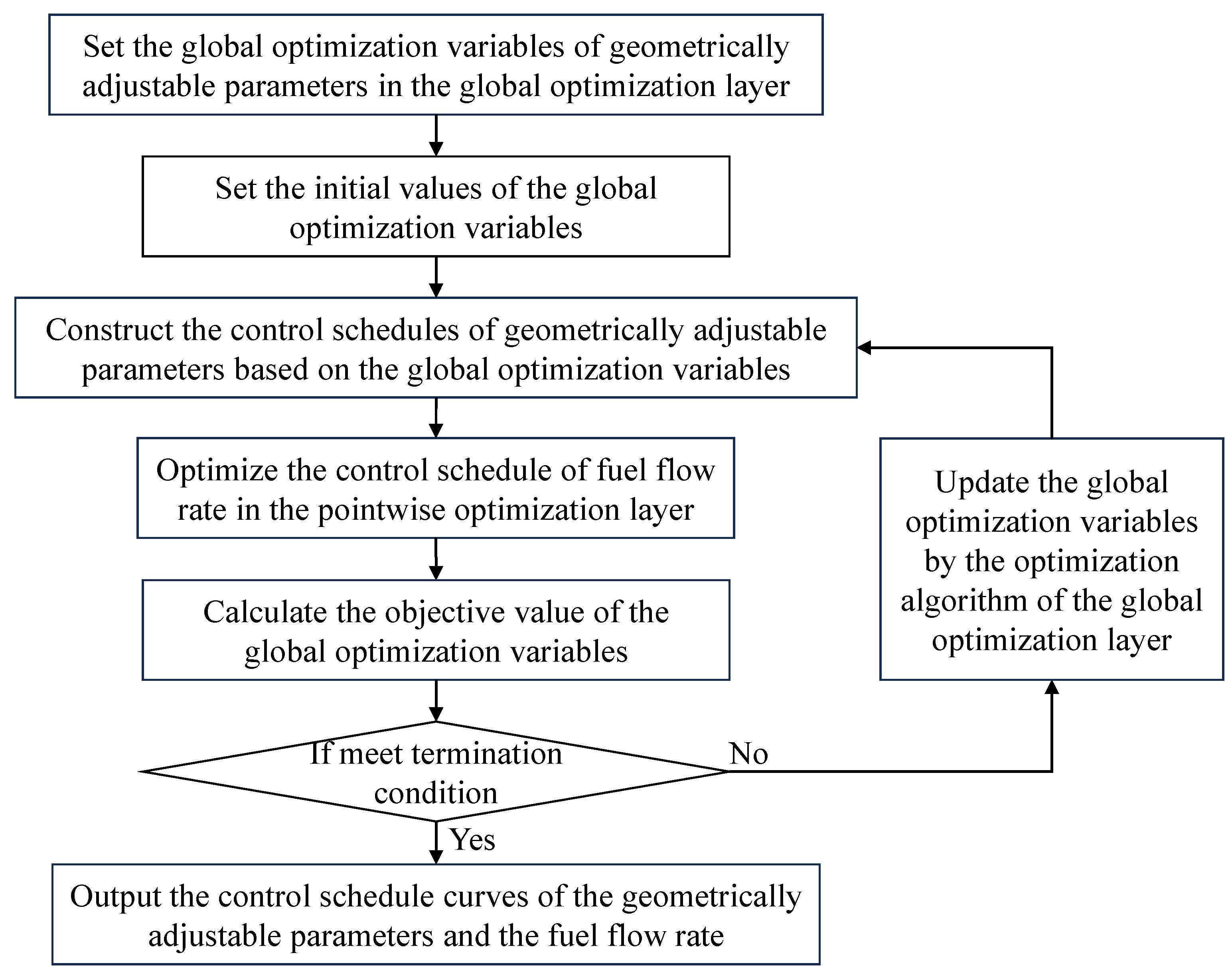
3. Combined Optimization Method

Generally, the fuel flow rate has a strong correlation with the transient performance of the engine. According to the results in references [12,13], even when the pointwise optimization method is adopted, the optimized control schedule of the fuel flow rate is quite smooth. Compared with the fuel flow rate, the geometrically adjustable parameters have a weaker correlation with the transient performance of the engine. Moreover, there is a strong coupling relationship among the geometrically adjustable parameters. According to the results in references [26,27], even when the global optimization method is adopted, the geometrically adjustable parameters will still fluctuate. Apparently, traditional optimization methods overlook the disparities among different adjustable parameters. They directly incorporate all adjustable parameters into the optimization variables, which imposes a heavy burden on the optimization algorithm and makes it very difficult to quickly optimize smooth control schedules.

The combined optimization method proposed in this paper divides the optimization of the dynamic control schedules into two layers. In the outer-layer optimization, the global optimization technique is applied to suppress the geometrically adjustable parameters that are prone to fluctuations. In the inner-layer optimization, the pointwise optimization technique is used to quickly obtain the control schedule of the fuel flow rate. Furthermore, the global optimization technology has been improved, which can significantly reduce the time cost of global optimization. The flowchart of the combined optimization method is shown in Figure 2.

Specifically, the combined optimization method involves the following steps:

(1)

Set the global optimization variables of geometrically adjustable parameters in the global optimization layer.

Generally, traditional global optimization methods uniformly divide the adjustable parameters into multiple control points according to time or rotor speed. For example, in Reference [27], the uniformly distributed control points for the Bezier curve of the nozzle throat area versus the high-pressure rotor speed are optimized, as shown in Figure 3. However, an excessive number of control points makes the dimension of global optimization extremely high, which greatly intensifies the difficulty of global optimization. In addition, the control schedules for engineering applications are required to be as simple as possible, so as to reduce the burden of the controller. In the case of uniformly distributed control points, the number of control points cannot be directly reduced. Otherwise, the degree of freedom of the control schedules will be limited. Therefore, a construction method for non-uniformly distributed control points is proposed.

In this paper, the low-pressure rotor speed $N_{\mathrm{L}}$ is selected as the independent variable of the control schedule. For the i-th adjustable parameter $x_i$, the non-uniform distribution of two control points is shown in Figure 4. If the coordinate values of the control points are directly taken as the optimization variables, the optimization algorithm cannot guarantee that the rotor speeds of the control points increase monotonically, i.e., $N_{\mathrm{L},2}>N_{\mathrm{L},1}$. Therefore, the dimensionless rotor speed increment is defined as optimization variable:

$$\lambda {\displaystyle {\sum }_{m=1}^{M+1}\Delta N_{\mathrm{L},m}}=N_{\mathrm{L},\mathrm{target}}-N_{\mathrm{L},\mathrm{start}}$$

(8)

where $\Delta N_{\mathrm{L},m}$ represents the m-th dimensionless rotor speed increment, which is within the interval (0, 1]; $N_{\mathrm{L},\mathrm{target}}$ and $N_{\mathrm{L},\mathrm{start}}$, respectively, represent the target and start value of the $N_{\mathrm{L}}$; $\mathit{M}$ represents the number of control points; and $\lambda$ represents the scaling factor.

When all the dimensionless rotor speed increments are known, the $\lambda$ can be calculated according to Equation (8). Thus, the rotor speeds of all control points can be calculated in turn:

$$N_{\mathrm{L},m}=N_{\mathrm{L},m-1}+\lambda \Delta N_{\mathrm{L},m}$$

(9)

where the subscript $m$ denotes the serial number of the control point. And it should be noted that $N_{\mathrm{L},0}=N_{\mathrm{L},\mathrm{start}}$.

Furthermore, to avoid sudden changes in the adjustable parameter, the change rate of the adjustable parameter is constrained. The change rate of the i-th adjustable parameter with respect to the rotor speed is defined as follows:

$${\dot{x}}_{i,m}=\left|{\displaystyle \frac{x_{i,m}-x_{i,m-1}}{N_{\mathrm{L},m}-N_{\mathrm{L},m-1}}}\right|$$

(10)

where $x_{i,m}$ represents the value of the i-th adjustable parameter of the m-th control point.

In order to complete the transition process rapidly, the adjustable parameter of the last control point will naturally approach its target value. Therefore, it is usually unnecessary to limit the change rate of the adjustable parameters between the last control point and the target point. However, if the coordinate values of the control points are directly taken as the optimization variables, the optimization algorithm cannot ensure that ${\dot{x}}_{i,m}$ of all control points are less than their limit value ${\dot{x}}_{i,\max }$.

When the values of $x_{i,m-1}$, $N_{\mathrm{L},m-1}$, and $N_{\mathrm{L},m}$ are all known, the upper and lower limits of $x_{i,m}$ can be calculated according to ${\dot{x}}_{i,\max }$:

$$\left\{\begin{array}{l}{x}_{i,m,\mathrm{up}}=x_{i,m-1}+{\dot{x}}_{i,\max }(N_{\mathrm{L},m}-N_{\mathrm{L},m-1})\\ x_{i,m,\mathrm{low}}=x_{i,m-1}-{\dot{x}}_{i,\max }(N_{\mathrm{L},m}-N_{\mathrm{L},m-1})\end{array}\right.$$

(11)

In addition, $x_{i,m}\in [x_{i,\mathrm{low}},x_{i,\mathrm{up}}]$. Evidently, $x_{i,m}\in [x_{i,\mathrm{low}},x_{i,\mathrm{up}}]\cap [x_{i,m,\mathrm{low}},x_{i,m,\mathrm{up}}]$. Therefore, the dimensionless value ${\overline{x}}_{i,m}$ of the adjustable parameter, which belongs to the interval [0, 1], is defined as the optimization variable. And the actual value of each adjustable parameter can be calculated in turn:

$$x_{i,m}={\overline{x}}_{i,m}\left(\min (x_{i,\mathrm{up}},x_{i,m,\mathrm{up}})-\max (x_{i,\mathrm{low}},x_{i,m,\mathrm{low}})\right)$$

(12)

In conclusion, the optimization variables of the i-th adjustable parameter can be expressed as the following:

$${\mathit{v}}_i=\left[(\Delta N_{\mathrm{L},1},{\overline{x}}_{i,1}),(\Delta N_{\mathrm{L},2},{\overline{x}}_{i,2}),\cdots ,(\Delta N_{\mathrm{L},m},{\overline{x}}_{i,m}),\cdots ,(\Delta N_{\mathrm{L},M},{\overline{x}}_{i,M}),\Delta N_{\mathrm{L},M+1}\right]$$

(13)

It should be noted that $\Delta N_{\mathrm{L},M+1}$ represents the dimensionless rotor speed increment between the last control point and the target point. Since the adjustable parameter of the target point is known, ${\overline{x}}_{i,M+1}$ does not need to be an optimization variable.

For each adjustable parameter, the number of control points $\mathit{M}$ can be different. And the global optimization variables of $\mathit{I}$ adjustable parameters in the global optimization layer can be described as follows:

$$\mathit{V}=\left[{\mathit{v}}_1,{\mathit{v}}_2,\cdots ,{\mathit{v}}_i,\cdots ,{\mathit{v}}_I\right]$$

(14)

By optimizing $\mathit{V}$, it can be ensured that the rotor speeds of the control points increase monotonically, and the change rate of the adjustable parameters does not exceed the limit.

(2)

Set the initial values of the global optimization variables.

If gradient optimization algorithms, such as the sequential quadratic programming algorithm, are used in the global optimization layer, it is assumed that the initial control points are uniformly distributed along the rotor speed, and the straight line connecting the start point and the target point of the transition process is used to determine the initial coordinates of the control points. For instance, regarding the two control points in Figure 4, their initial positions are shown in Figure 5. Therefore, the value of $\Delta N_{\mathrm{L},m}$ for each initial control point can be set to the same value of $1/(1+M)$, where $\mathit{M}$ represents the number of control points. Subsequently, the value of ${\overline{x}}_{i,m}$ for each control point can be calculated inversely in sequence according to Equation (12).

If population-based algorithms like the differential evolution algorithm are used in the global optimization layer, each individual representing global optimization variables only needs to be randomly initialized within the optimization region. In addition, to give the initial population relatively reasonable initial values, the initialization method used in gradient optimization algorithms can be adopted to initialize a single individual in the population. Generally, the number of individuals in a population is relatively large. Assigning an initial value to a single individual will not affect the diversity of the initial population and, thus, will not affect the convergence of the algorithm.

(3)

Construct the control schedules of geometrically adjustable parameters based on the global optimization variables.

When the global optimization variables are given, the coordinate values of each control point can be calculated according to Equations (9) and (12). The results of Reference [26] show that the piecewise linearization of the control schedule has little impact on the transition performance. Therefore, in order to reduce the complexity of the control schedule, this paper no longer constructs complex curves such as the Bezier curve based on the control points. Instead, the control schedule of each adjustable parameter is directly constructed through linear interpolation of the control points.

(4)

Optimize the control schedule of fuel flow rate in the pointwise optimization layer.

In the pointwise optimization layer, the control schedules of geometrically adjustable parameters delivered by the global optimization layer are adopted. During each time step of the transition process, the fuel flow rate is optimized to meet Equation (4).

It should be noted that at this time, the $\mathit{X}(t_k)$ in Equation (4) only contains one optimization variable, that is, the fuel flow. Therefore, gradient optimization algorithms such as the sequential quadratic programming algorithm can be adopted to ensure relatively high optimization efficiency. We strongly recommend using the sequential quadratic programming algorithm in the pointwise optimization layer, as it is extremely proficient in solving the nonlinear constrained optimization problem described by Equation (4). During the optimization process, the algorithm will automatically search for the optimal solution within the feasible region that satisfies the constraints, without requiring any additional treatment of the constraint conditions.

(5)

Calculate the objective value of the global optimization variables.

The objective function described in Equation (2) needs to be integrated over time. Its discretized form over time steps is shown as follows:

$$\min O={\displaystyle {\sum }_{k=1}^K{\left(P(\mathit{X}(t_k))-P_{\mathrm{target}}\right)}^2}$$

(15)

where $K$ represents the number of time steps.

The control point construction method proposed in this paper has considered the change rate constraints of geometrically adjustable parameters, and the pointwise optimization layer has considered engine performance constraints. Thus, there is no need to account for other constraint conditions in the global optimization layer’s objective function.

Particularly, for the case of interruption in the transition process calculation, it is stipulated that the engine performance parameters at subsequent time steps are equal to their interruption values. At this moment, a relatively large objective function value will cause the optimization algorithm to discard current optimization variables.

(6)

Check whether the termination condition of the global optimization layer is met.

The termination condition of the global optimization layer is associated with the optimization algorithm used in this layer. When gradient optimization algorithms such as the sequential quadratic programming algorithm are used, the termination condition is usually that the change in the objective function value is less than a predefined threshold. When population-based algorithms like the differential evolution algorithm are employed, the termination condition is usually that the number of optimization generations reaches its predetermined value.

If the termination condition is met, output the control schedule curves of the geometrically adjustable parameters and the fuel flow rate. Otherwise, update the global optimization variables by the optimization algorithm of the global optimization layer and then, return to step 3.

In conclusion, the combined optimization method proposed in this paper can integrate the advantages of the global optimization methods and the pointwise optimization methods. In the pointwise optimization layer, the only optimization variable is the fuel flow rate. The sequential quadratic programming algorithm is adopted to ensure relatively high optimization efficiency [30]. In the global optimization layer, the non-uniform control points construction method proposed in this paper can significantly reduce the number of control points, thus, greatly shortening the time required for global optimization. The differential evolution algorithm [31], which has good global convergence, is applied to the global optimization layer, thus ensuring that the algorithm is less likely to fall into local optimal solutions.

4. Results and Discussion

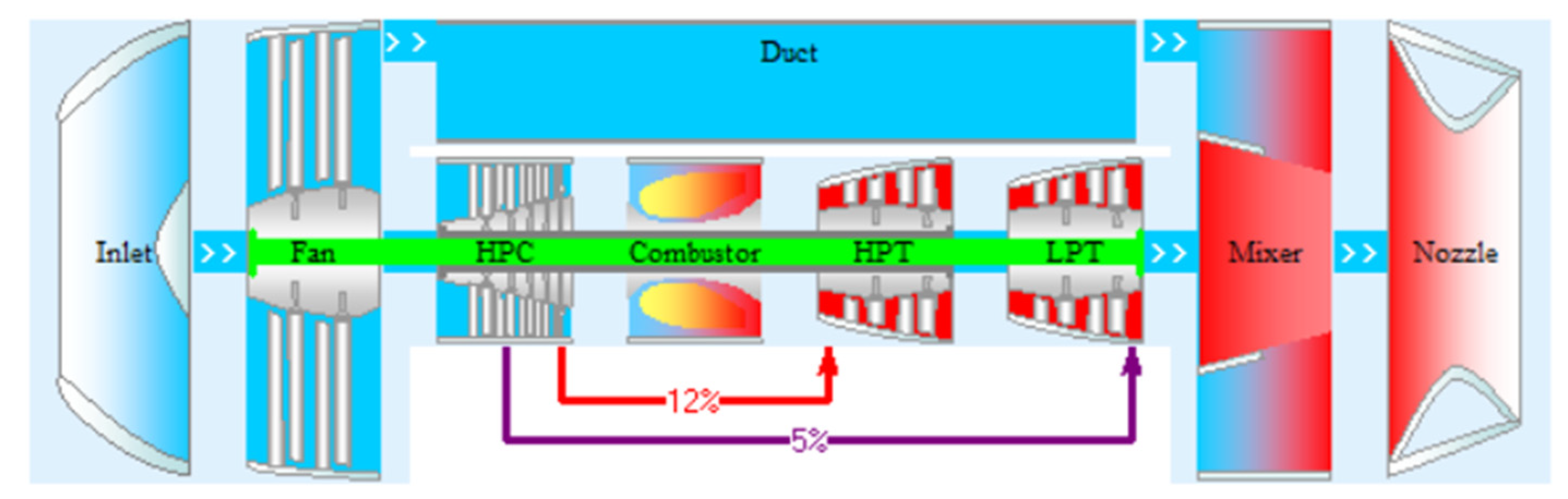
4.1. Simulation Model

To verify the effectiveness of the combined optimization method, the acceleration and deceleration control schedules of a mixed-flow turbofan engine were optimized. The simulation model of the mixed-flow turbofan engine was built in the aero-engine performance simulation program [32,33,34], as shown in Figure 6. This engine model is a detailed model (controller not included) constructed based on the component-based method. The performance parameters of each component model are calculated based on theoretical equations and characteristic maps constructed using experimental data. In Figure 6, HPC represents the high-pressure compressor, while HPT and LPT stand for the high-pressure turbine and low-pressure turbine, respectively. Lines of different colors denote the bleed air, and the numbers represent the relative bleed air amounts.

The design parameters of the mixed-flow turbofan engine are given in

Table 1. Design parameters of the mixed-flow turbofan engine.

Design Parameter	Value
Altitude (m)	0
Mach number	0
Inlet mass flow rate (kg/s)	130
Fan pressure ratio	3.32
Fan bypass ratio	0.59
HPC pressure ratio	6.00
Combustor outlet temperature (K)	1976
Thrust (kN)	93.0
Specific fuel consumption (kg/(N·h))	0.0767

, as well as the design operating condition is the sea-level standard condition.

Before optimizing the control schedules, it is necessary to determine the start and final states of the transition process. The two states selected in this paper are the idle state and the maximum state at the sea-level standard condition, and their parameters are shown in

Table 2. Parameters of idle state and maximum state.

Parameter Name	Idle State	Maximum State
Altitude (m)	0	0
Mach number	0	0
$\mathrm{Fuel} \mathrm{flow} \mathrm{rate} {\mathit{W}}_{\mathrm{f}}$ (kg/s)	0.1315	1.9854
$\mathrm{LPT} \mathrm{throat} \mathrm{area} A_{\mathrm{LPT}}$ (%)	130	100
$\mathrm{Nozzle} \mathrm{throat} \mathrm{area} A_8$ (m2)	0.5	0.2846
$\mathrm{Low}-\mathrm{pressure} \mathrm{rotor} \mathrm{speed} N_{\mathrm{L}}$ (%)	48	100
Thrust (kN)	5.06	93.0
Specific fuel consumption (kg/(N·h))	0.0936	0.0767

.

In this paper, two geometrically adjustable parameters, the LPT throat area and the nozzle throat area $A_8$, are selected as the optimization variables for the global optimization layer, while the fuel flow rate $W_{\mathrm{f}}$ is chosen as the optimization variable for the pointwise optimization layer. The lower and upper limits of the optimization variables are shown in

Table 3. Lower and upper limits of the optimization variables.

Optimization Variable	Lower Limit	Upper Limit
$A_{\mathrm{LPT}}$ (%)	100	130
$A_8$ (m2)	0.2	0.5
$W_{\mathrm{f}}$ (kg/s)	0.05	3

. The limit values of the constraint parameters to be satisfied during the transition process are shown in

Table 4. Limit values of the constraint parameters.

Constraint Parameter	Lower Limit	Upper Limit
$\mathrm{Fan} \mathrm{surge} \mathrm{margin} {\mathrm{SM}}_{\mathrm{F}}$ (%)	15
$\mathrm{HPC} \mathrm{surge} \mathrm{margin} {\mathrm{SM}}_{\mathrm{C}}$ (%)	15
$\mathrm{Low}-\mathrm{pressure} \mathrm{rotor} \mathrm{speed} N_{\mathrm{L}}$ (%)		102
$\mathrm{High}-\mathrm{pressure} \mathrm{rotor} \mathrm{speed} N_{\mathrm{H}}$ (%)		102
$\mathrm{Combustor} \mathrm{outlet} \mathrm{temperature} T_4$ (K)		2000
$\mathrm{Duct} \mathrm{outlet} \mathrm{Mach} \mathrm{number} M{a}_{22}$		0.8
$\mathrm{Change} \mathrm{rate} \mathrm{of} W_{\mathrm{f}}$ with respect to time (kg/s2)		1.5
$\mathrm{Change} \mathrm{rate} \mathrm{of} A_{\mathrm{LPT}}$$\mathrm{with} \mathrm{respect} \mathrm{to} N_{\mathrm{L}}$ (%/%)		20
$\mathrm{Change} \mathrm{rate} \mathrm{of} A_8$$\mathrm{with} \mathrm{respect} \mathrm{to} N_{\mathrm{L}}$ (m2/%)		0.5

.

In the pointwise optimization layer, the time step for the transition process calculation is set to 0.1 s. The total time of the acceleration and deceleration processes are set to 6 s and 10 s, respectively. The convergence accuracy of the sequential quadratic programming algorithm is set to 10⁻⁴. In the global optimization layer, the population size of the differential evolution algorithm is set to eight times the number of optimization variables. When the number of control points of the control schedules is 1, 2, and 3, respectively, the maximum number of generations of the differential evolution algorithm is set to 80, 100, and 150, respectively.

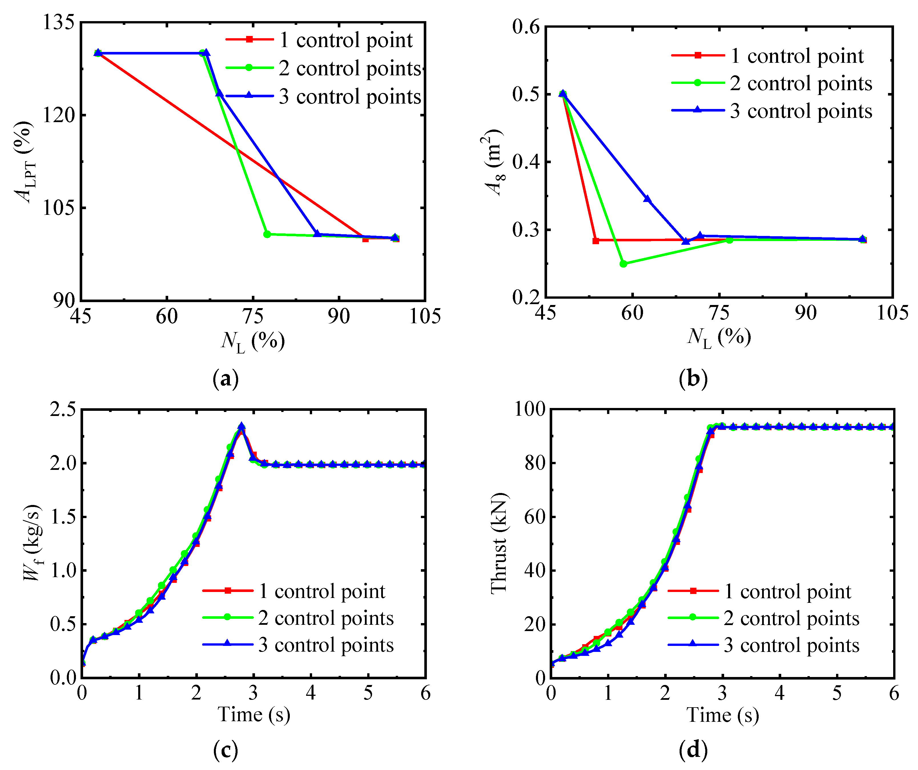
4.2. Research on the Number of Control Points

As mentioned above, the combined optimization method proposed in this paper enables the control schedules with a smaller number of control points. To analyze the impact of the number of control points on the transition process, 1–3 control points are selected for each geometrically adjustable parameter, respectively, and the control schedules for the transition process are optimized. The optimization results of the acceleration and deceleration processes are presented in Figure 7 and Figure 8, respectively.

It can be seen from Figure 7a,b that when the number of control points varies, the optimization results of the control schedules for geometrically adjustable parameters differ substantially. However, as can be seen from Figure 7c,d, the number of control points has no obvious impact on the fuel flow rate and acceleration time. The reason is that, compared with the fuel flow rate, geometrically adjustable parameters have a relatively minor impact on the acceleration process. Moreover, there exists a coupling relationship among geometrically adjustable parameters. That is, different combinations of these parameters can achieve the same control effect. Therefore, there exist different control schedules for geometrically adjustable parameters, yet similar transition processes can be achieved through similar fuel flow rate control schedules. In addition, an increase in the number of control points makes the feasible region of the control schedule more diverse. This is the main reason why geometrically adjustable parameters obtained by traditional optimization methods tend to fluctuate.

The deceleration process depicted in Figure 8 is similar to the acceleration process. Therefore, to simplify the control schedules and suppress their fluctuations, a single control point is selected for all geometrically adjustable parameters in both the acceleration and deceleration processes in this paper. Apparently, compared with traditional global optimization methods, which often use as many as 30 control points for a single adjustable parameter [27], the number of control points in this paper is significantly reduced, thus significantly improving the efficiency of global optimization.

In addition, the optimization times of the combined optimization method with different numbers of control points and the pointwise optimization method are shown in

Table 5. The optimization times of the combined optimization method with different numbers of control points and the pointwise optimization method.

Optimization Case	Acceleration Optimization Time	Deceleration Optimization Time
Combined optimization with 1 control point	2.5 h	3.1 h
Combined optimization with 2 control points	7.6 h	9.6 h
Combined optimization with 3 control points	20.0 h	23.7 h
Pointwise optimization	30 s	37 s

. It should be noted that the hardware platform used for the optimization is a computer with a CPU with a main frequency of 2.53 GHz and 8 GB of RAM. As can be seen from Table 5, with the reduction in the number of control points, the optimization time of the combined optimization method decreases significantly. However, even when the combined optimization method uses only one control point, its optimization time is still significantly longer than that of the pointwise optimization method. Evidently, although the pointwise optimization method is prone to fluctuations in the control schedules, its high optimization efficiency cannot be ignored. This is also the intention behind proposing the combined optimization method in this paper.

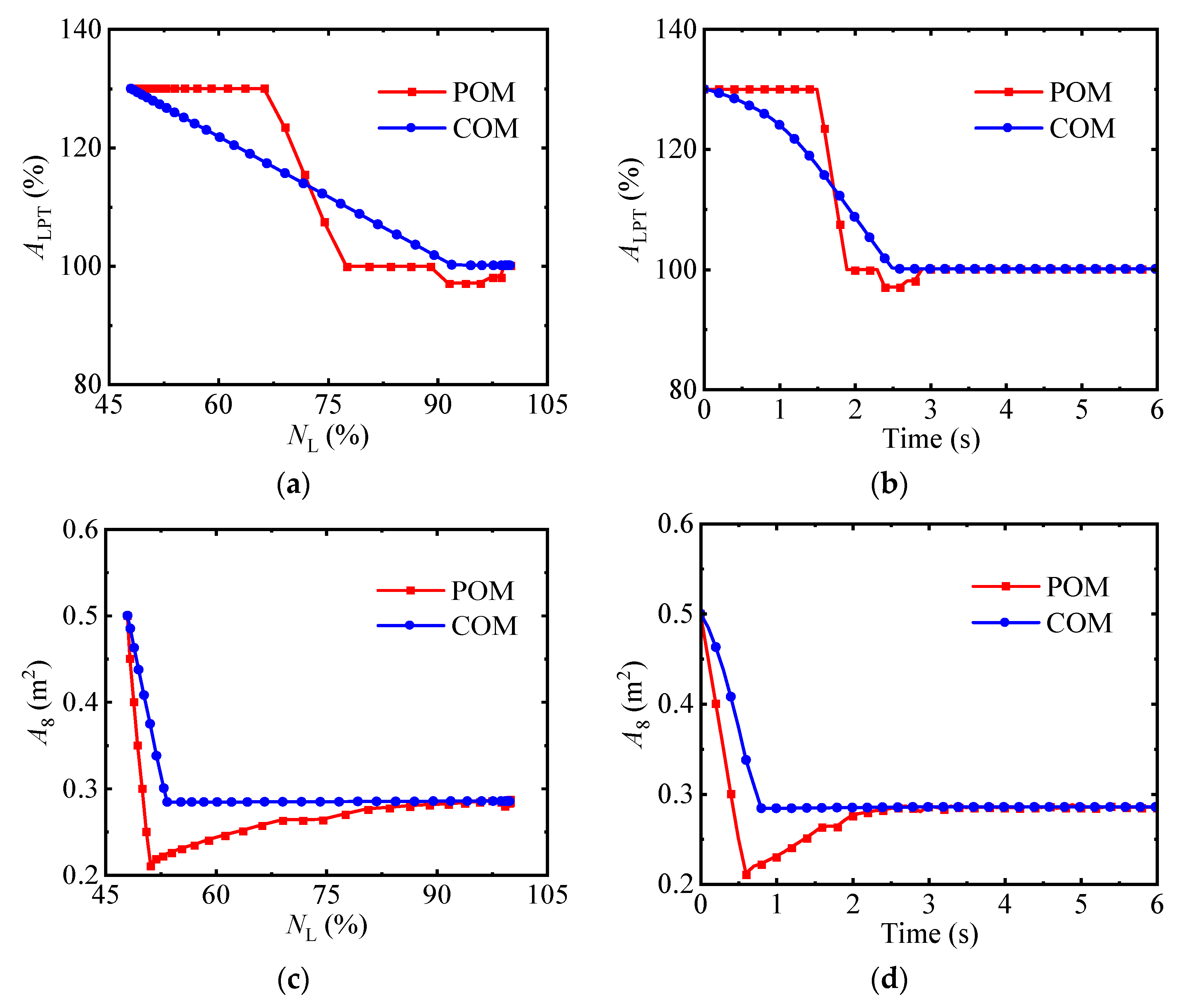
4.3. The Optimization Results of the Acceleration Process

Figure 9 and Figure 10 show the variation trends of adjustable parameters and performance parameters in the acceleration process optimized by the pointwise optimization method (POM) and the combined optimization method (COM). In Figure 9, on the left, the adjustable parameters’ variation trends with $N_{\mathrm{L}}$ are shown (adjustable parameters are usually controlled according to rotor speed), while on the right are those with time. As can be observed from Figure 9a–d, the geometrically adjustable parameters optimized by POM fluctuate significantly, while those optimized by COM are relatively smooth. In the first 2 seconds, the value of $A_8$ optimized by POM is relatively small, while $A_{\mathrm{LPT}}$ is relatively large, resulting in a relatively small pressure ratio of the low-pressure turbine. Therefore, a slightly larger $W_{\mathrm{f}}$ is required to increase the thrust rapidly, as shown in Figure 9e,f. After 2 seconds, the adjustable parameters optimized by the two methods are relatively close to each other.

It can be seen from Figure 10 that there is no obvious difference in the transition times obtained by the two optimization methods, and the variation trends of the performance parameters, except for the ${\mathrm{SM}}_{\mathrm{F}}$ and the $M{a}_{22}$, are very similar. This is due to the fact that before 2 seconds, the value of $A_8$ optimized by COM is relatively large, which makes the engine’s flow capacity stronger, thereby, making the ${\mathrm{SM}}_{\mathrm{F}}$ and $M{a}_{22}$ relatively larger as well. Sufficient ${\mathrm{SM}}_{\mathrm{F}}$ can avoid fan surge caused by sudden changes in working conditions during the acceleration process, which is beneficial for the safety of the engine.

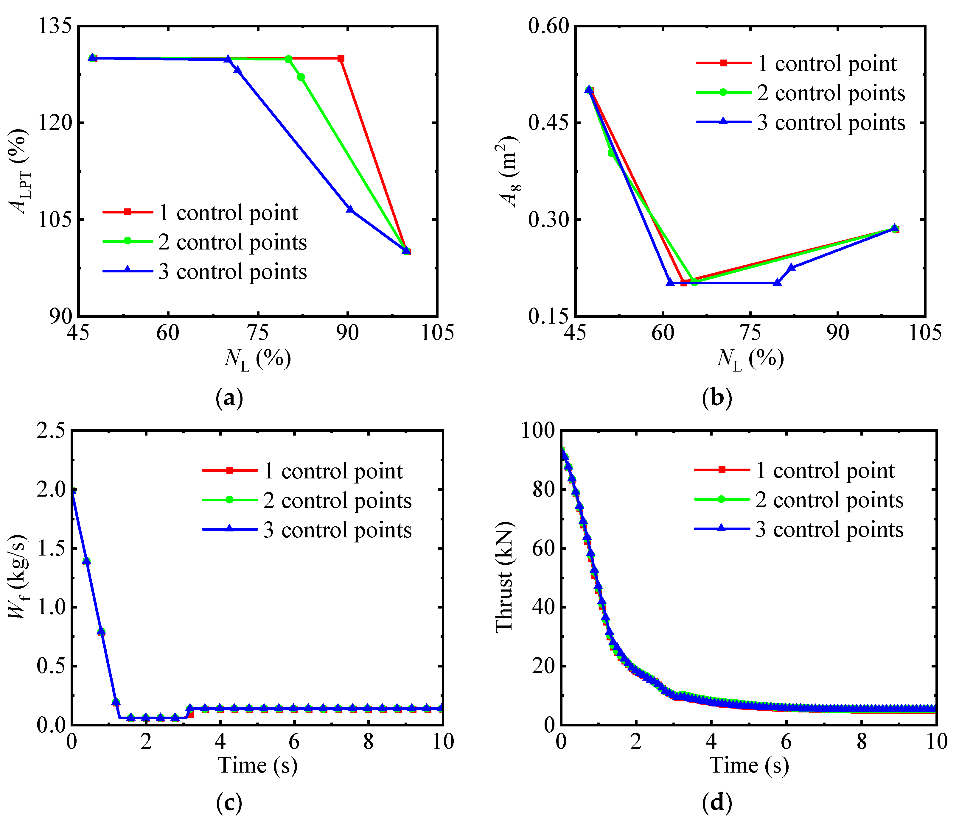
4.4. The Optimization Results of the Deceleration Process

Figure 11 and Figure 12 show the variation trends of adjustable parameters and performance parameters in the deceleration process optimized by the pointwise optimization method (POM) and the combined optimization method (COM). In Figure 11, on the left, the adjustable parameters’ variation trends with $N_{\mathrm{L}}$ are shown (adjustable parameters are usually controlled according to rotor speed), while on the right are those with time. By comparing Figure 9a–d and Figure 11a–d, it can be seen that during the deceleration process, the fluctuation of the geometrically adjustable parameters optimized by POM is more evident, while those optimized by COM remain relatively simple. Limited by the maximum value of the $W_{\mathrm{f}}$ change rate and the minimum value of the $W_{\mathrm{f}}$, the variation trends of the $W_{\mathrm{f}}$ optimized by the two methods during the deceleration process are almost exactly the same, as shown in Figure 11f. In the first four seconds, the value of $A_8$ optimized by POM is relatively large, while $A_{\mathrm{LPT}}$ is relatively small, which makes the pressure ratio of the low-pressure turbine relatively large. Therefore, the $N_{\mathrm{L}}$ optimized by POM is slightly higher than that by COM in the first four seconds, as shown in Figure 11e and Figure 12c. After 4 seconds, the adjustable parameters optimized by both methods approach their target values rapidly.

It can be seen from Figure 12 that there is no obvious difference in the transition times obtained by the two optimization methods, and the variation trends of the performance parameters, except for the ${\mathrm{SM}}_{\mathrm{F}}$ and the $M{a}_{22}$, are very similar. This is due to the fact that before 2 seconds, the value of $A_8$ optimized by COM is relatively small, which makes the engine’s flow capacity weaker, and thus the ${\mathrm{SM}}_{\mathrm{F}}$ and $M{a}_{22}$ are also smaller. Although in the early stage of the deceleration process, the ${\mathrm{SM}}_{\mathrm{F}}$ obtained by COD is smaller, it does not approach its limit value, so it will not cause obvious adverse effects on the safety of the engine. In addition, in the early stage of the deceleration process, the $M{a}_{22}$ obtained by POM reaches its limit value, which makes the duct operate under its working boundary. It is evident that COM can balance the working conditions of the fan and duct components effectively.

In conclusion, during the acceleration and deceleration process, there is always a situation where the performance parameters optimized by POM touch the limit values, while the parameters optimized by COM are still far from the limit boundaries, as shown in Figure 10e and Figure 12h. This is due to the fact that POM fully exploits the performance of the engine at each time step in order to minimize the acceleration time, but it also causes some engine components to operate under extreme conditions. However, COM is restricted by the change rate constraints of the control points of geometrically adjustable parameters and cannot adjust the geometrically adjustable parameters arbitrarily. It can not only suppress the fluctuation of the control schedules, but also prevent some components from becoming too close to their working boundaries.

5. Conclusions

In this paper, a combined optimization method for the transition control schedules of aero-engines was proposed. This method integrates the traditional pointwise optimization method into the global optimization method. In addition, the problem of a large number of control points that needed to be optimized in global optimization methods was solved. The research results showed the following:

(1)

Compared with the fuel flow rate, geometrically adjustable parameters have a relatively minor impact on the transition process. Moreover, there exists a coupling relationship among geometrically adjustable parameters. That is, different combinations of these parameters can achieve the same control effect. This is the main reason why geometrically adjustable parameters obtained by traditional optimization methods tend to fluctuate. This is also the reason why the transition time does not change significantly after the smoothing technologies are applied to the control schedules.

(2)

In the global optimization layer of the combined optimization method, the number of control points has no obvious impact on the transition time. The fewer the number of control points, the more beneficial it is not only for reducing the optimization time but also for avoiding fluctuations in the control schedules.

(3)

There is no significant difference in the transition time optimized by the combined optimization method and the pointwise optimization method. However, the control schedules obtained by the combined optimization method are not only free from fluctuations but also simple, making them highly applicable in engineering.

(4)

Constrained by change rate constraints of the control points of geometrically adjustable parameters, the combined optimization method cannot adjust the geometrically adjustable parameters arbitrarily. This enables the optimized control schedules to prevent some components from becoming too close to their working boundaries, thus, enhancing the safety of the engine during the transition process.

In future research, the combined optimization method can be applied to new-concept engines with more adjustable parameters, thus, further verifying the effectiveness of this method. In addition, in combination with the engineering requirements of the control schedules, further simplifications can be made to the construction method of control points of the control schedules, thus, reducing the optimization difficulty and cost of the control schedules.

References

1. Chen, H.; Li, Q.; Ye, Z.; Pang, S. Neural Network-Based Parameter Estimation and Compensation Control for Time-Delay Servo System of Aeroengine. Aerospace 2025, 12, 64. [Google Scholar] [CrossRef]
2. Lian, X.C.; Wu, H. Aeroengine Principles; Northwestern Polytechnical University Press: Xi’an, China, 2005; p. 300. [Google Scholar]
3. Hao, W.; Wang, Z.; Zhang, X.; Zhang, M. A New Design Method for Mode Transition Control Law of Variable Cycle Engine. In Proceedings of the AIAA 2018 Joint Propulsion Conference, Cincinnati, OH, USA, 9 July 2018. [Google Scholar]
4. Zheng, J.; Luo, Y.; Tang, H.; Zhang, J.; Chen, M.; Zhang, Y. Design Method Research of Mode Switch Transient Control Schedule on Adaptive Cycle Engine. J. Propuls. Technol. 2022, 43, 49–58. [Google Scholar]
5. Chen, Y.; Xu, S.; Cai, Y.; Tu, Q. Virtual Power Extraction Method of Designing Acceleration and Deceleration Control Law of Turbofan. In Proceedings of the 45th AIAA/ASME/SAE/ASEE Joint Propulsion Conference & Exhibit, Denver, CO, USA, 2–5 August 2009. [Google Scholar]
6. Chen, Y.; Xu, S.; Liu, Z.; Tu, Q.Y.; Yu, S.Z. Power Extraction Method for Acceleration and Deceleration Control Law Design of Turbofan Engine. J Aerosp. Power. 2009, 24, 867–874. [Google Scholar]
7. Jia, L.Y.; Chen, Y.C.; Tan, T.; Tian, T.G. Analysis for Influence of Variable Geometry Parameters on Transition State Performance of Variable Cycle Engine. J. Propuls. Technol. 2020, 41, 1681–1691. [Google Scholar]
8. Kurzke, J.; Halliwell, I. Propulsion and Power; Springer: Berlin, Germany, 2018; pp. 270–273. [Google Scholar]
9. Jia, L.Y. Research on Variable Cycle Engine Control Schedule Design. Ph.D. Thesis, Northwestern Polytechnical University, Xi’an, China, 2017. [Google Scholar]
10. Jia, L.Y.; Chen, Y.C.; Cheng, R.H.; Song, K.; Tan, T. Direct Simulation Method of Transient-State Performance of Variable Cycle Engines. J. Aeronaut. 2020, 41, 123901. [Google Scholar]
11. Jia, L.; Chen, Y.; Cheng, R.; Tan, T.; Song, K. Designing Method of Acceleration and Deceleration Control Schedule for Variable Cycle Engine. Chin. J. Aeronaut. 2021, 34, 27–38. [Google Scholar] [CrossRef]
12. Lu, J.; Guo, Y.Q.; Wang, L. A New Method for Designing Optimal Control Law of Aeroengine in Transient States. J. Aerosp. Power 2012, 27, 1914–1920. [Google Scholar]
13. Qi, X.F.; Fan, D.; Chen, Y.C.; Li, W.G. Multivariable Optimal Acceleration Control of Turbofan Engine Based on FSQP Algorithm. J. Propuls. Technol. 2004, 25, 233–236. [Google Scholar]
14. Li, J.; Fan, D.; Sreeram, V. Optimization of Aero Engine Acceleration Control in Combat State Based on Genetic Algorithms. Int. J. Turbo Jet-Eng. 2012, 29, 29–36. [Google Scholar] [CrossRef]
15. Hu, H. Transient Control of Aeroengine Based on SQP Method. Master’s Thesis, Nanjing University of Aeronautics and Astronautics, Nanjing, China, 2015. [Google Scholar]
16. Jiang, T.M.; Zhang, X.B.; Wang, Z.X.; Liu, Y.Q. Design of Control Law Design of Lift Fan Starting Based on Time Prediction. J. Aerosp. Power 2023, 38, 2001–2014. [Google Scholar]
17. Dai, A.N. Research on the On-Board Adaptive Model and Optimization Control of Aero-Engine. Master’s Thesis, Dalian University of Technology, Dalian, China, 2020. [Google Scholar]
18. Liu, Z.H. Research on Optimizing Adaptive Acceleration and Deceleration Control Schedule of Turbofan Engine. Master’s Thesis, Nanjing University of Aeronautics and Astronautics, Nanjing, China, 2021. [Google Scholar]
19. Zhu, B.B. Design of Control Schedule and Control Algorithm for Triple Bypass Variable Cycle Engine. Master’s Thesis, Nanjing University of Aeronautics and Astronautics, Nanjing, China, 2020. [Google Scholar]
20. Zheng, Q.G.; Zhang, H.B. A Global Optimization Control for Turbo-Fan Engine Acceleration Schedule Design. Proc. Inst. Mech. Eng. Part G J. Aerosp. Eng. 2018, 232, 308–316. [Google Scholar] [CrossRef]
21. Zhao, L.; Fan, D.; Shan, W.W. A Global Optimization Approach to Aero-Engine Under Transient Conditions. J. Aerosp. Power 2007, 22, 1200–1203. [Google Scholar]
22. Hao, W.; Wang, Z.X.; Zhang, X.B.; Li, Z.; Wang, J.K. Ground starting modeling and control law design method of variable cycle engine. J. Aerosp. Power 2022, 37, 152–164. [Google Scholar]
23. Hao, W.; Wang, Z.X.; Zhang, X.B.; Li, Z.; Wang, J.K. Mode Transition Modeling and Control Law Design Method of Variable Cycle Engine. J. Propuls. Technol. 2022, 43, 78–87. [Google Scholar]
24. Zhang, J.Y.; Dong, P.C.; Zheng, J.C.; Wang, J.; Chen, M. General Design Method of Control Law for Adaptive Cycle Engine Mode Transition. AIAA J. 2022, 60, 330–344. [Google Scholar] [CrossRef]
25. Zhang, X.; Ye, Y.; Wang, Z.; Xiao, B. A Neural Network Learning-Based Global Optimization Approach for Aero-Engine Transient Control Schedule. Neurocomputing 2022, 469, 180–188. [Google Scholar] [CrossRef]
26. Song, K.R.; Chen, Y.C.; Jia, L.Y.; Tan, T. Design of Variable Cycle Engine Acceleration Control Schedule Based on Gradient Method and Maximum Entropy Method. J. Propuls. Technol. 2022, 43, 55–63. [Google Scholar]
27. Ye, Y.F.; Wang, Z.X.; Zhang, X.B. Cascade Ensemble-RBF-Based Optimization Algorithm for Aero-Engine Transient Control Schedule Design Optimization. Aerosp. Sci. Technol. 2021, 115, 106779. [Google Scholar] [CrossRef]
28. Ye, Y.F.; Wang, Z.X.; Zhang, X.B. Multi-Surrogates Based Modelling and Optimization Algorithm Suitable for Aero-Engine. J. Propuls. Technol. 2021, 42, 2684–2693. [Google Scholar]
29. Ye, Y.F.; Wang, Z.X.; Zhang, X.B. Sequential Ensemble Optimization Based on General Surrogate Model Prediction Variance and Its Application on Engine Acceleration Schedule Design. Chin. J. Aeronaut. 2021, 34, 16–33. [Google Scholar] [CrossRef]
30. Yuan, X.Y.; Sun, W.Y. Optimal Theory and Methods; Beijing Science and Technology Press: Beijing, China, 2001. [Google Scholar]
31. Storn, R.; Price, K. Differential Evolution-A Simple and Efficient Heuristic for Global Optimization over Continuous Spaces. J. Glob. Optim. 1997, 11, 341–359. [Google Scholar] [CrossRef]
32. Zhou, H. Research on Variable Cycle Engine Characteristics Analysis and Its Integration Design with Aircraft. Ph.D. Thesis, Northwestern Polytechnical University, Xi’an, China, 2016. [Google Scholar]
33. Zhang, M.Y.; Wang, Z.X.; Zhang, X.B.; Zhou, L. Simulation of Windmilling-Ram Mode Performance for Tandem TBCC Engine. J. Aerosp. Power 2018, 33, 2939–2949. [Google Scholar]
34. Hao, W.; Wang, Z.X.; Zhang, X.B.; Zhou, L. Acceleration Technique for Global Optimization of a Variable Cycle Engine. Aerosp. Sci. Technol. 2022, 129, 107792. [Google Scholar] [CrossRef]
Figure 1. Working lines of the compressor.
Aerospace 12 00144 g001
Figure 2. Flowchart of the combined optimization method.
Aerospace 12 00144 g002
Figure 3. Control points for the Bezier curve.
Aerospace 12 00144 g003
Figure 4. Non-uniform distribution of two control points.
Aerospace 12 00144 g004
Figure 5. Uniform distribution of the two initial control points.
Aerospace 12 00144 g005
Figure 6. Simulation model of the mixed-flow turbofan engine.
Aerospace 12 00144 g006
Figure 7. The parameters of the acceleration process obtained by the combined optimization method with different numbers of control points. (a) A LPT vs. N L , (b) A 8 vs. N L , (c) W f vs. Time, (d) Thrust vs. Time.
Aerospace 12 00144 g007
Figure 8. The parameters of the deceleration process obtained by the combined optimization method with different numbers of control points. (a) A LPT vs. N L , (b) A 8 vs. N L , (c) W f vs. Time, (d) Thrust vs. Time.
Aerospace 12 00144 g008
Figure 9. Variation trends of adjustable parameters in the acceleration process. (a) A LPT vs. N L , (b) A LPT vs. Time, (c) A 8 vs. N L , (d) A 8 vs. Time, (e) W f vs. N L , (f) W f vs. Time.
Aerospace 12 00144 g009aAerospace 12 00144 g009b
Figure 10. Variation trends of performance parameters in the acceleration process. (a) Thrust vs. Time, (b) Specific fuel consumption vs. Time, (c) N L vs. Time, (d) N H vs. Time, (e) SM F vs. Time, (f) SM C vs. Time, (g) T 4 vs. Time, (h) M a 22 vs. Time.
Aerospace 12 00144 g010aAerospace 12 00144 g010b
Figure 11. Variation trends of adjustable parameters in the deceleration process. (a) A LPT vs. N L , (b) A LPT vs. Time, (c) A 8 vs. N L , (d) A 8 vs. Time, (e) W f vs. N L , (f) W f vs. Time.
Aerospace 12 00144 g011
Figure 12. Variation trends of performance parameters in the deceleration process. (a) Thrust vs. Time, (b) Specific fuel consumption vs. Time, (c) N L vs. Time, (d) N H vs. Time, (e) SM F vs. Time, (f) SM C vs. Time, (g) T 4 vs. Time, (h) M a 22 vs. Time.
Aerospace 12 00144 g012