Heuristic Deepening of the Variable Cycle Engine Model Based on an Improved Volumetric Dynamics Method

Abstract

High-precision and real-time modeling are crucial for accelerating the research cycle of next-generation aero-engines. The volumetric dynamics method is acknowledged as the most accurate approach to capture the engine’s transition state process. Nevertheless, the traditional volumetric method encounters challenges, such as neglecting static pressure equilibrium within the mixer and complexities in ascertaining the component volume size when the dynamic simulation time step varies. To address these issues, an improved volumetric dynamics modeling method featuring pressure ratio collaborative updating and the adaptive virtual volume method has been proposed, and a real-time component-level model of a variable cycle engine is established based on this method. The pressure ratio collaborative updating method dynamically updates the pressure ratio of rotating components by inversely calculating the internal and external bypass pressure of the mixer according to static pressure equilibrium constraints and the momentum conservation principle. The adaptive virtual volume method determines the optimal virtual volume size using the particle swarm optimization algorithm, with cosine similarity serving as the evaluation metric. The simulation results indicate that the model based on an improved volumetric dynamics method achieves high accuracy and superior real-time performance. Moreover, compared to traditional modeling methods, the co-operating line of the improved volumetric dynamic method exhibits a smoother transition, signifying a closer resemblance to the real physical process.

1. Introduction

The variable cycle engine, as a pivotal system for next-generation fighter aircraft, adeptly reconciles the economic efficiency of subsonic flight with the substantial thrust requirements of supersonic flight, offering unparalleled performance benefits [1,2]. High-precision dynamic models serve as the cornerstone for engine control [3] and fault diagnosis [4], and are crucial in ensuring the performance advantage [5,6].

At present, aero-engine modeling methods are primarily divided into three categories: data-driven, mechanism-driven [7,8,9], and hybrid models. Data-driven modeling approaches regard the engine as an integrated system, constructing a model that mirrors the engine’s functionality through analysis of its input and output data. The two main methodologies are system identification methods [10,11] and black-box methods [12,13]. With the development of machine learning, the method of constructing aero-engine models based on neural networks has been widely applied. Ren et al. proposed a data-driven modeling method for the aero-engine aerodynamic model by combining stochastic gradient descent with support vector regression (SGDSVR) [14]. Quevedo et al. proposed a surrogate model based on artificial neural networks (ANNs) to estimate the fundamental frequency of the assembly formed by the wind turbine. Both of the data-driven modeling methods offer clear advantages in terms of real-time performance [15]. However, the established model may struggle to accurately capture the dynamic characteristics of each section parameter. Mechanism-based modeling methods can be used to develop full-envelope and full-state component-level models based on the principles of aerothermodynamics, and are extensively utilized in the field of aero-engine modeling [16]. The hybrid model integrates the advantages of models using both the artificial intelligence method and the mechanism-based method. Pang et al. proposed a novel hybrid adaptive model, which consists of a component-level model, an improved incremental linearized Kalman filter, and a state space model [17]. Cheng et al. combined the component-level model (CLM) with an artificial neural network (ANN) to establish a surrogate model, which has good real-time performance [18]. Cai et al. proposed a new hybrid modeling framework that combines a long short-term memory (LSTM) neural network with a physics-based model, which demonstrates better performance than traditional methods [19]. As can be seen from the above research, hybrid models usually combine other methods with the mechanistic-based models. Therefore, the mechanism-based model is the cornerstone for developing aero-engine modeling, and its development and research are of vital importance. The primary solution methods for these models encompass the iterative method [20,21] and volumetric dynamics method [22,23].

Early iterative algorithms primarily included the parameter cycle method and the equilibrium cycle method, both characterized by their simplicity and ease of implementation. However, the complexity of aero-engine configurations continues to escalate, and these methods have difficulties in meeting real-time performance requirements. In response to this challenge, more advanced algorithms, such as the N + 1 point residual method, Newton–Raphson method, and Broyden method have been developed [24]. Among these methods, the Newton–Raphson method has emerged as one of the most prevalently utilized in the field of aero-engine performance simulation, owing to its characteristics of high computational efficiency and excellent convergence [25,26]. Nevertheless, it is worth noting that, since iterative methods solely rely on mathematical mechanisms, part of the transient characteristics may be overlooked during the solution process.

The volumetric dynamics method was first proposed by Fawke, who states that the assumption of mass flow rate continuity during transient processes is invalid, and the accumulation effect of the air flow rate and energy will cause pressure fluctuations of the volume outlet [27]. Subsequently, Roberts developed a non-iterative turbofan engine model that integrates the principles of rotor dynamics, thermodynamics, and volumetric dynamics mechanisms. This model provides more details of the engine operational process, thereby enhancing the comprehension of its performance characteristics [28]. Yepifanov et al. investigated the impact of various dynamic factors on volumetric method modeling, and the established engine model can more accurately reflect the dynamic operating characteristics of the engine [29]. Masahiro Kurosaki et al. proposed a numerical integration method for the aero-engine volumetric model based on an improved Euler method [30]. Liu et al. combined the volume effect with an iteration algorithm, presenting a novel modeling method for variable area bypass injectors. This method has been proven to exhibit superior convergence and computational efficiency [31]. Guo et al. developed a reusable and flexible general simulation platform for turbofan engines based on a multi-dynamics approach; the simulation result has minimal steady-state error and good real-time performance [32]. In the component-level model (CLM) based on the volume effect, the dynamic characteristics of an engine can be captured more accurately without iteration through reasonable design of the volumes. Although the volumetric dynamics method for modeling has become relatively mature, challenges still persist. These challenges include insufficient consideration of static pressure balance conditions in the mixer and difficulties in selecting appropriate volume sizes during variable step dynamic performance calculations. These problems have an important impact on improving the accuracy and real-time performance of the engine model.

The main innovations of this study are as follows:

(1)

A pressure ratio collaborative update method is proposed to address the oversight of the static pressure balance constraint at the mixer in conventional volumetric models.

(2)

An adaptive virtual volume method is proposed to improve the model’s real-time performance while preserving the dynamic advantages of the volumetric dynamic method.

(3)

Based on the proposed improved volumetric dynamic method, the component-level model of the variable cycle engine is established. The model can capture the actual physical characteristics of the VCE more accurately.

It is worth mentioning that this paper further clarified the differences and advantages of the iterative method and volumetric dynamic method in modeling, which has great significance for the future development of aero-engine modeling.

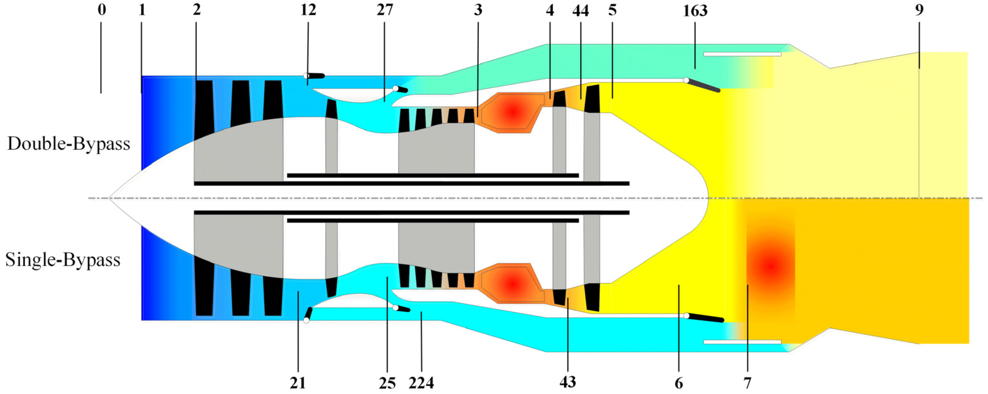
2. Component-Level Modeling

2.1. Modeling Hypothesis

The variable cycle engine (VCE), renowned for its superior performance characteristics, including exceptional fuel efficiency during subsonic cruise and remarkable unit thrust in supersonic flight regimes, has emerged as a prominent focus of advanced research. The VCE, characterized by its intricate configuration and pronounced inter-component coupling, is selected as the research subject to effectively demonstrate the universal applicability of the proposed methodology. Spanning from inlet to outlet, the components of the VCE primarily include the inlet, fan, forward variable area bypass injector (FVABI), core driven fan stage (CDFS), high-pressure compressor (HPC), combustion chamber, high-pressure turbine (HPT), mode selection valve (MSV), low-pressure turbine (LPT), rear variable area bypass injector (RVABI), mixer, afterburner, and nozzle. The main architecture and cross-section definition are shown in Figure 1.

The actual operating process of the VCE is extremely complex, making the establishment of an accurate mathematical model quite challenging. Therefore, the following assumptions are often made before modeling:

(1)

The gas within the engine flow path is treated as a quasi one-dimensional flow.

(2)

The effects of variations in the gas Reynolds number on component characteristics are disregarded.

(3)

The adiabatic coefficient $k$ at each section of the engine is regarded as a function of total temperature $T_t$ and residual gas coefficient $\alpha$ at that section.

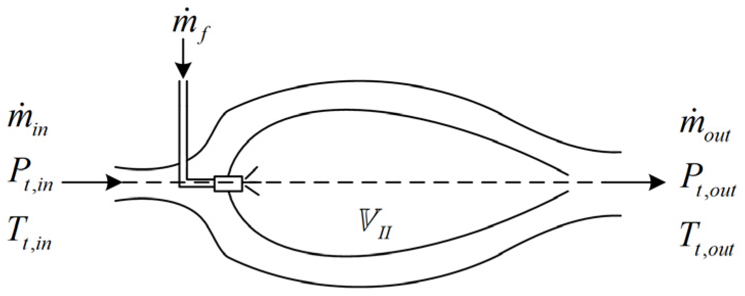
2.2. Volume Modeling

Taking the combustion chamber as an example, this section provides a concise introduction of the volume modeling. The inlet and outlet cross-sections of the combustion chamber volume are defined as Figure 2.

According to the energy equation, the unsteady processes in the main combustion chamber caused by volume effects can be described as Equations (1) and (2) [33].

$$\begin{array}{l}{\displaystyle \frac{d{T}_{t,out}\left(t\right)}{dt}}={\displaystyle \frac{R_{out}\left(t\right)T_{t,out}\left(t\right)}{V_C{P}_{t,out}\left(t\right){\psi }_h\left(t\right)}}\cdot \left[{\dot{m}}_f\left(t\right)\left({\eta }_C\left(t\right)H_f+h_f\left(t\right)-{\displaystyle \frac{h_{out}\left(T_{t,out}\left(t\right),{\alpha }_{out}\left(t\right)\right)}{k_{out}\left(T_{t,out}\left(t\right),{\alpha }_{out}\left(t\right)\right)}}\right)\right.+\\ {\dot{m}}_{in}\left(t\right)\left(h_{in}\left(T_{t,in}\left(t\right)\right)-{\displaystyle \frac{h_{out}\left(T_{t,out}\left(t\right),{\alpha }_{out}\left(t\right)\right)}{k_{out}\left(T_{t,out}\left(t\right),{\alpha }_{out}\left(t\right)\right)}}\right)\\ -{\dot{m}}_{out}\left(t\right)\cdot \left.\left({\displaystyle \frac{k_{out}\left(T_{t,out}\left(t\right),{\alpha }_{out}\left(t\right)\right)-1}{k_{out}\left(T_{t,out}\left(t\right),{\alpha }_{out}\left(t\right)\right)}}{h}_{out}\left(T_{t,out}\left(t\right),{\alpha }_{out}\left(t\right)\right)\right)\right]\end{array}$$

(1)

$${\displaystyle \frac{d{P}_{t,out}\left(t\right)}{dt}}={\displaystyle \frac{R_{out}\left(t\right)T_{t,out}\left(t\right)}{V_C}}\left[{\dot{m}}_{in}\left(t\right)+{\dot{m}}_f\left(t\right)-{\dot{m}}_{out}\left(t\right)\right]+{\displaystyle \frac{P_{t,out}\left(t\right)}{T_{t,out}\left(t\right)}}{\displaystyle \frac{d{T}_{t,out}\left(t\right)}{dt}}$$

(2)

where ${\psi }_h$ is an enthalpy coefficient, as shown in Equation (3).

$${\psi }_h\left(t\right)=d{\displaystyle \frac{h_{out}\left(T_{t,out}\left(t\right),{\alpha }_{out}\left(t\right)\right)}{k_{out}\left(T_{t,out}\left(t\right),{\alpha }_{out}\left(t\right)\right)}}/d{T}_{t,out}\left(t\right)$$

(3)

To avoid differential operations, the calculation of ${\psi }_h$ uses Equation (4).

$${\psi }_h\left(t\right)={\displaystyle \frac{1}{2}}\left({\displaystyle \frac{h_{out}\left(T_{t,out}\left(t\right)+1,{\alpha }_{out}\left(t\right)\right)}{k_{out}\left(T_{t,out}\left(t\right)+1,{\alpha }_{out}\left(t\right)\right)}}\right.-\left.{\displaystyle \frac{h_{out}\left(T_{t,out}\left(t\right)-1,{\alpha }_{out}\left(t\right)\right)}{k_{out}\left(T_{t,out}\left(t\right)-1,{\alpha }_{out}\left(t\right)\right)}}\right)$$

(4)

After using the Euler method to discretize, the update of total temperature and total pressure of the volume outlet cross-section is shown in Equations (5) and (6).

$$T_{t,out}\left(t\right)=T_{t,out}\left(t-1\right)+{\displaystyle \frac{d{T}_{t,out}\left(t\right)}{dt}}dt$$

(5)

$$P_{t,out}\left(t\right)=P_{t,out}\left(t-1\right)+{\displaystyle \frac{d{P}_{t,out}\left(t\right)}{dt}}dt$$

(6)

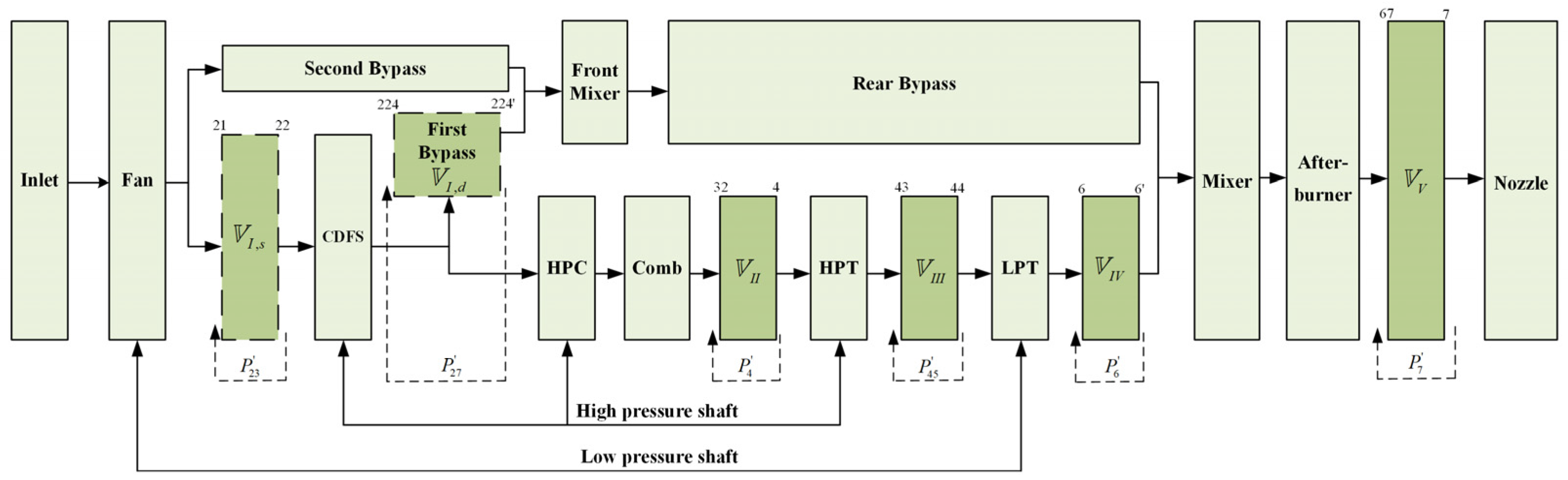
2.3. Component-Level Model

During the transition state process of the VCE, the fuel flow rate within the combustion chamber undergoes alterations. The HPT is influenced by the outlet temperature of the combustion chamber, causing its output power to vary. The fluctuation subsequently affects the operating point of the CDFS and HPC. Similarly, the output power of the LPT is also affected by the variations of inlet temperature, causing the FAN operating point variations. As a result, the operating matching points of the engine will shift. When dynamically modeling, it is essential to meet the requirements for updating each component output parameter.

Component-level modeling of the VCE primarily consists of component modeling modules and engine matching modules. The component modeling modules are established based on the principle of aerothermodynamics; the detailed modeling process is outlined in reference [34], and this part will not be repeated. The engine matching module is predominantly established based on iterative methods or volumetric dynamic methods. The convergence of the engine model based on the iterative method is heavily reliant on the selection of initial guess values, which primarily consists of rotating the component pressure ratio and rotor speed. For VCE, the initial guess values are typically set as: $\left[\begin{array}{ccccccc}{\pi }_{FAN}& {\pi }_{CDFS}& {\pi }_{HPC}& {\pi }_{HPT}& {\pi }_{LPT}& n_L& n_H\end{array}\right]$. The complexity of engine structures leads to an increase in the number of initial guess values, which adversely affects both the convergence and real-time performance of the model. When modeling based on the volumetric dynamics method, iteration can be avoided by setting the volume appropriately. The specific selection criteria for the volume are as follows:

(1)

Can avoid the iteration solutions for related components’ outlet parameters;

(2)

Can accurately capture the high-frequency characteristics of the engine’s transient state processes;

(3)

Can reflect the accumulation effects resulting from mass and energy;

(4)

Can demonstrate the impact of actuator variations on engine performance.

According to the characteristics of the VCE, this study selects five volumes, and the inlet and outlet cross-sections are shown as Figure 3. Volume I is primarily utilized to coordinate the fan outlet pressure. Due to the different thermodynamic cycles in various operating modes of the VCE, the selection of Volume I also differs. In single-bypass mode, with the MSV closed, the transition section between the fan and CDFS is designated as Volume I ${𝕍}_{I,s}$ to regulate the fan pressure ratio. In double-bypass mode, where air flow circulates through the second bypass, the first bypass is selected as Volume I ${𝕍}_{I,d}$ to adjust the CDFS pressure ratio. Volumes II to IV are employed to adjust the pressure ratio of the HPC, HPT, and LPT, respectively. The outlet pressure of each volume is updated during each flow path calculation, and the pressure ratio of rotating components is further adjusted to prevent the need for iteration. The following takes the double-bypass mode as an example to explain the updating process of each component in detail.

In double-bypass mode, the air flow from the first bypass and second bypass is blended together in the front mixer. Volume I ${𝕍}_{I,d}$ is positioned at the first bypass, with the inlet cross-section selected as $224$ and the outlet cross-section designated as ${224}^{\prime }$. The outlet total pressure $P_{t{224}^{\prime }}$ and total temperature $T_{t{224}^{\prime }}$ of ${𝕍}_{I,d}$ are adjusted based on the volume model established in Section 2.2, and $P_{t{224}^{\prime }}$ is also used to update the CDFS outlet pressure. Note that Formula (7) shows how the outlet parameters of the components in front of the volume are modifed, not the volume import.

$$P_{t27}^{\prime }\left(t\right)=P_{t{224}^{\prime }}\left(t\right)/{\sigma }_1$$

(7)

The accumulation of mass and energy in the combustion chamber leads to significant volumetric effects, necessitating to set a volume within it. To ensure that the complex combustion effects are not taken into account when the volume is updated, the front part of combustion chamber is calculated according to thermodynamic principles, Volume II ${𝕍}_{II}$ is situated in the rear part of the combustion chamber, with the inlet cross-section at $32$ and the outlet cross-section at $4$. The outlet total pressure $P_{t4}$ and total temperature $T_{t4}$ of ${𝕍}_{II}$ are adjusted based on the volume model, and $P_{t4}$ is also used to update the outlet total pressure $P_{t3}^{\prime }$ of HPC.

$$P_{t3}^{\prime }\left(t\right)=P_{t4}\left(t\right)/{\sigma }_2$$

(8)

The HPT outlet temperature is relatively high, which means that the volumetric effects resulting should be considered. Volume III ${𝕍}_{III}$ is set between the HPT and LPT, with the inlet cross-section at 43 and outlet cross-section at 44. After adjusting the outlet total pressure $P_{t44}$ and total temperature $T_{t44}$ of ${𝕍}_{III}$, $P_{t44}$ is used to update the outlet pressure $P_{t42}^{\prime }$ of the HPT.

$$P_{t42}^{\prime }\left(t\right)=P_{t44}\left(t\right)/{\sigma }_3$$

(9)

The outlet air flow from the LPT merges with the air flow from the rear bypass at mixer, so Volume IV ${𝕍}_{IV}$ is positioned at the inlet of the mixer’s inner to reflect the volume effect. The inlet cross-section is 6 and outlet cross-section is $6^{\prime }$. After adjusting the outlet total pressure $P_{t{6}^{\prime }}$ and total temperature $T_{t{6}^{\prime }}$ of ${𝕍}_{IV}$, $P_{t{6}^{\prime }}$ is used to update the outlet pressure of LPT.

$$P_{t5}^{\prime }\left(t\right)=P_{t{6}^{\prime }}\left(t\right)/{\sigma }_4$$

(10)

To reflect the volumetric effects caused by mass and energy accumulation in the afterburner and the impact of the nozzle throat area $A_8$ on the engine’s performance, Volume V ${𝕍}_V$ is positioned in the rear section of afterburner, with the inlet cross-section at 67 and outlet cross-section at 7. The outlet total pressure $P_{t7}$ is used to update the mixer outlet pressure $P_{t65}^{\prime }$, and the fan and CDFS will also be affected.

$$P_{t65}^{\prime }\left(t\right)=P_{t7}\left(t\right)/{\sigma }_5$$

(11)

After a complete flow path calculation, the inlet and outlet pressures of rotating components are updated, and the pressure ratio $\pi$ used for interpolation in characteristic maps is adjusted accordingly. As the model approaches a steady state, the fluctuations of temperature and pressure in the volumes tend to zero, and the parameters of each component will no longer change.

3. Improved Volumetric Dynamics Method

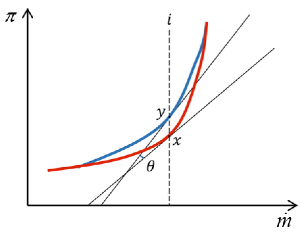
3.1. Pressure Ratio Collaborative Updating Method

As shown in Figure 3, Volume IV ${𝕍}_{IV}$ and Volume I ${𝕍}_{I,d}$ in double-bypass mode are positioned adjacent to the mixer. It is imperative to account for the impact of static pressure within the inner and outer channels to correct the gas flow rate of the volume. Taking Volume IV as an example, the inner air flow rate can be expressed as Equation (12).

$${\dot{m}}_6={\dot{m}}_5{\displaystyle \frac{P_{s6}}{P_{s16}}}$$

(12)

As illustrated in Equation (12), during a quasi-steady state of the engine, the gas flow tends to stabilize, and there is no accumulation of mass flow within the volume, indicating that the static pressure at the mixer is balanced. However, during a transient state of the engine, it is difficult to maintain the static pressure balance in the mixer. At the same time, pressure fluctuations caused by volumetric effects in Volume V ${𝕍}_V$ are only propagated to the outer bypass in the traditional volumetric dynamic model. As a result, Volume V is used solely to adjust the CDFS pressure ratio in single-bypass mode, while in double-bypass mode it is used to adjust the fan pressure ratio. Nonetheless, in the actual operating process, when nozzle throat area $A_8$ opens and other control parameters remain constant, the LPT pressure ratio increases, resulting in an elevation of output power, an increase in low-pressure rotor speed, and a shift in the operating points of both the fan and LPT. This change also has some effect on the high-pressure shaft. Therefore, relying on Volume V to adjust the fan or CDFS pressure ratio is insufficient.

To more precisely describe the physical operating process of the engine, this section proposes a pressure ratio collaborative updating method. The pressure fluctuations generated in Volume V propagate upstream simultaneously through both the inner and outer culverts, adjusting the pressure ratios of the rotating components. As these fluctuations pass through the mixer, the static pressure balance is assumed to determine the distribution of the air flow rate between the internal and external bypass. The basic concept of the pressure ratio collaborative updating method is shown in Figure 4.

After adjusting the total outlet pressure $P_{t7}$ of Volume V ${𝕍}_V$ based on the volume model, the resulting pressure fluctuations propagate upstream to update the mixer outlet total pressure $P_{t65}$. The mixer combine two air flow streams into a single stream, so it is challenging to directly ascertain the inlet total pressures $P_{t6}$ and $P_{t163}$ based on the outlet total pressure $P_{t65}$. In this study, considering the physical characteristics of momentum conservation and the constraints of the static pressure balance, the values of $P_{t6}$ and $P_{t163}$ can be determined through reverse calculation. According to the momentum conservation equation shown in Equation (13), the external value of the mixer inlet total pressure $P_{t163}$ can be obtained. Then, Equations (14) and (15) are used to calculate the static pressures of both the internal inlet $P_{s6}$ and the external inlet $P_{s16}$, respectively. By assessing the equilibrium of static pressures, the internal value of the mixer inlet total pressure $P_{t6}$ can be accurately determined based on the bisection iterative method.

$$P_{t163}={\displaystyle \frac{P_{t65}f\left({\lambda }_{65}\right)\left(A_6+A_{163}\right)-P_{t6}f\left({\lambda }_6\right)A_6}{f\left({\lambda }_{163}\right)A_{163}}}$$

(13)

$$P_{s163}=P_{t163}{\left(1-{\displaystyle \frac{k_{163}-1}{k_{163}-1}}{\lambda }_{163}^2\right)}^{k_{163}/\left(k_{163}-1\right)}$$

(14)

$$P_{s6}=P_{t6}{\left(1-{\displaystyle \frac{k_6-1}{k_6-1}}{\lambda }_6^2\right)}^{k_6/\left(k_6-1\right)}$$

(15)

The solution $P_{t6}$ can further adjust the drop pressure ratio of the low-pressure turbine ${\pi }_{LPT}$, while $P_{t163}$ is transmitted upstream through the rear bypass to update the outlet pressure of the front mixer. The update and solution method for the front mixer is the same as mixer, and the inlet total pressure $P_{t13}$ and $P_{t224}$ can be determined based on Equations (16)–(18).

$$P_{t13}={\displaystyle \frac{P_{t15}f\left({\lambda }_{15}\right)\left(A_{224}+A_{13}\right)-P_{t224}f\left({\lambda }_{224}\right)A_{224}}{f\left({\lambda }_{13}\right)A_{13}}}$$

(16)

$$P_{s13}=P_{t13}{\left(1-{\displaystyle \frac{k_{13}-1}{k_{13}-1}}{\lambda }_{13}^2\right)}^{k_{13}/\left(k_{13}-1\right)}$$

(17)

$$P_{s224}=P_{t224}{\left(1-{\displaystyle \frac{k_{224}-1}{k_{224}-1}}{\lambda }_{224}^2\right)}^{k_{224}/\left(k_{224}-1\right)}$$

(18)

The total pressure $P_{t224}$ is transmitted through the first bypass to adjust the pressure ratio of CDFS. Meanwhile, the total pressure $P_{t13}$ modifies the fan’s pressure ratio through the second bypass. In double-bypass mode, Volume V ${𝕍}_V$ can achieve a coordinated update of ${\pi }_{Fan},{\pi }_{CDFS},{\pi }_{LPT}$. In single-bypass mode, although no airflow passes through the second bypass, the pressure fluctuations also have a significant impact on CDFS, and ${𝕍}_V$ can still achieve a coordinated update of ${\pi }_{CDFS}$ and ${\pi }_{LPT}$. The model considering the pressure ratio collaborative updating not only maintains the static pressure balance constraint condition at the mixer, but also takes into account the influence of variable geometry adjustment on the dynamic matching of upstream components.

3.2. Adaptive Virtual Volume Method

The real-time performance and simulation accuracy of aero-engine dynamic models have long been critical indicators for evaluating model quality. Generally, models based on the iteration method support larger dynamic simulation time steps (20–25 ms), resulting in better real-time performance, and models based on volume dynamics can reflect the engine high-frequency physical characteristics more accurately with smaller simulation time steps (1–2 ms) [35]. Traditional volume-based models typically use smaller steps, which will compromise real-time performance. Increasing the simulation time step may improve real-time performance to some extent, but risks losing the model’s dynamic tracking capability. Under the same control parameters, for a deceleration process with total a simulation time of 10 s, the Newton–Raphson iteration model ${\mathrm{CLM}}_{N-R}$ uses a simulation time step of 25 ms, while the improved volumetric dynamics model ${\mathrm{CLM}}_{Im𝕍}$ uses steps of 1 ms, 2 ms, 5 ms, and 10 ms. The fan co-operating line and corresponding computational time are compared as shown in Figure 5. The computational time was tested on a desktop computer with an i5-12400 CPU and a dominant frequency of 2.50 GHz.

As shown in Figure 5, as the simulation time step increases, the co-operating line of the volumetric dynamics model progressively deviates from the normal line, while the computational time significantly decreases. This indicates a contradictory relationship between real-time performance and the dynamic tracking capability. This paper also found that, in addition to the simulation time step, the selection of volume size also has a significant impact on the dynamic simulation results of the volumetric dynamics model. By adjusting the size of the virtual volume, the decline in dynamic tracking capability resulting from the increased simulation time step can be partially alleviated.

To assess the quality of the selected volume size, a benchmark model and evaluation metric must first be established. In the traditional volumetric dynamics model, the simulation time step is set to 1 ms. Following this, the volume size is adjusted to ensure that the dynamic co-operating lines of the rotating components are as smooth as possible, thereby establishing the benchmark model. Cosine similarity is used to measure the difference between two individuals by comparing the cosine of the angle between their vectors. When the simulation time step changes, the average cosine similarity between the dynamic co-operating lines of the current model and benchmark model are calculated to assess the fit degree. The selection rule of the vector angle is shown in Figure 6, where the red curve represents the dynamic co-operating line of the benchmark model and the blue curve represents the dynamic operating line of the current model.

The average cosine similarity is calculated as shown in Equation (19).

$$\cos \left(\theta \right)={\displaystyle \frac{1}{n}}\left[{\displaystyle \frac{{\displaystyle \sum _{i=1}^n\left({\dot{m}}_{xi}\times {\dot{m}}_{yi}+{\pi }_{xi}\times {\pi }_{yi}\right)}}{{\displaystyle \sum _{i=1}^n\left(\sqrt{{\dot{m}}_{xi}^2+{\pi }_{xi}^2}\times \sqrt{{\dot{m}}_{yi}^2+{\pi }_{yi}^2}\right)}}}\right]$$

(19)

where the subscript $x$ represents points on the co-operating line of the benchmark model, while the subscript $y$ represents points on the co-operating line of the current model at the same air flow rate $i$. The value of $\theta$ is the angle between the two points’ tangents. The closer the result is to 1, the higher the fit degree.

When changing the simulation time step, adjusting the size of the volume can still affect the performance matching of the entire engine. Furthermore, the influence of each volume size on the transient state process demonstrates a complex coupling relationship. Therefore, it is necessary to optimize the sizes of all virtual volumes collectively. Particle swarm optimization (PSO) is an algorithm designed to discover optimal solutions through co-operation and information-sharing mechanisms within a population. In this section, the PSO algorithm is used to determine the optimal virtual volume sizes for different simulation time steps.

Under the same operating conditions and control parameters, the simulation time step for the benchmark model is consistently set to 1 ms, while the current model represents the improved volume dynamics model, which is achieved through modification of the simulation time step. These models perform dynamic performance simulations, yielding different co-operating lines. The average cosine similarity is calculated by taking $n$ points uniformly according to the air flow rate on the co-operating line, as shown in Equation (19). The sum of average cosine similarities for the fan, CDFS, HPC, HPT, and LPT is used as the objective function. The optimization criterion is shown in Equation (20).

$$J=\cos {\left(\theta \right)}_{Fan}+\cos {\left(\theta \right)}_{CDFS}+\cos {\left(\theta \right)}_{HPC}+\cos {\left(\theta \right)}_{HPT}+\cos {\left(\theta \right)}_{LPT}$$

(20)

The optimization objective is obtained by calculating the cosine similarity weighted sum of the current co-operating line and the benchmark co-operating line of the fan, CDFS, HPC, HPT, and LPT. The larger the average cosine similarity, the closer the dynamic co-operating line of current model to benchmark model, indicating better performance.

4. Simulation and Analysis

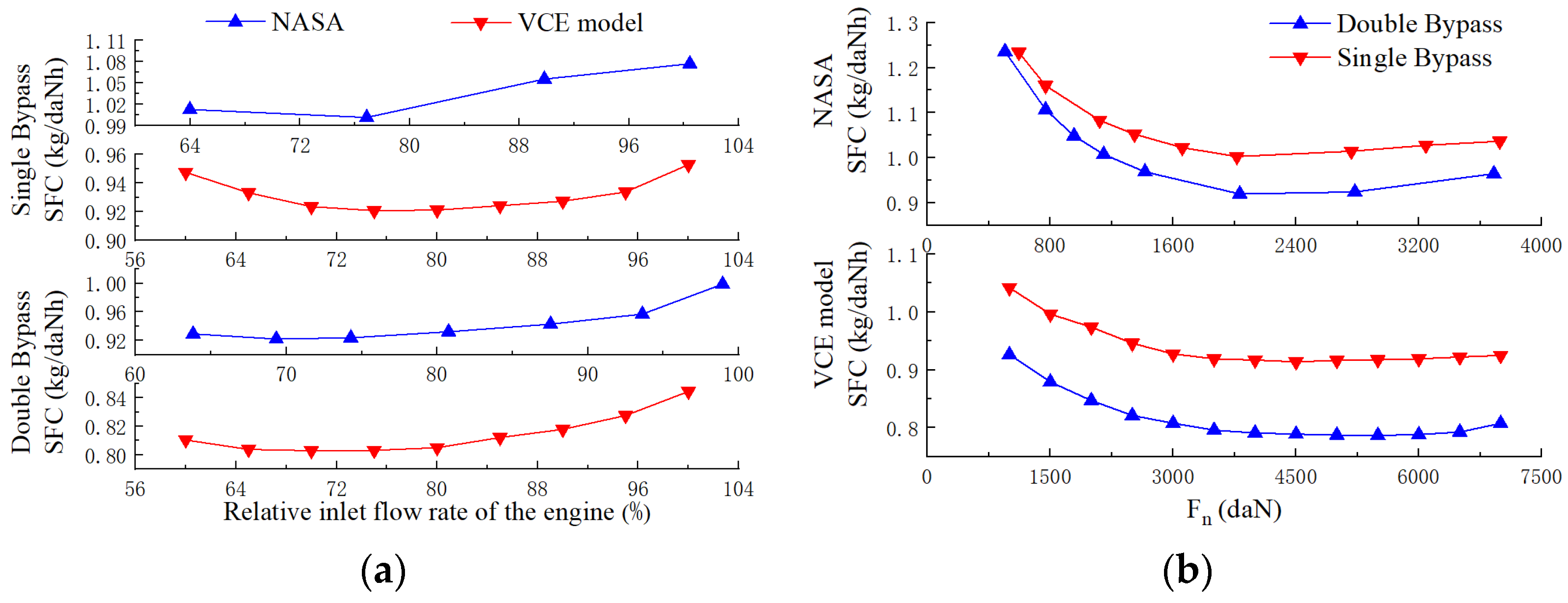
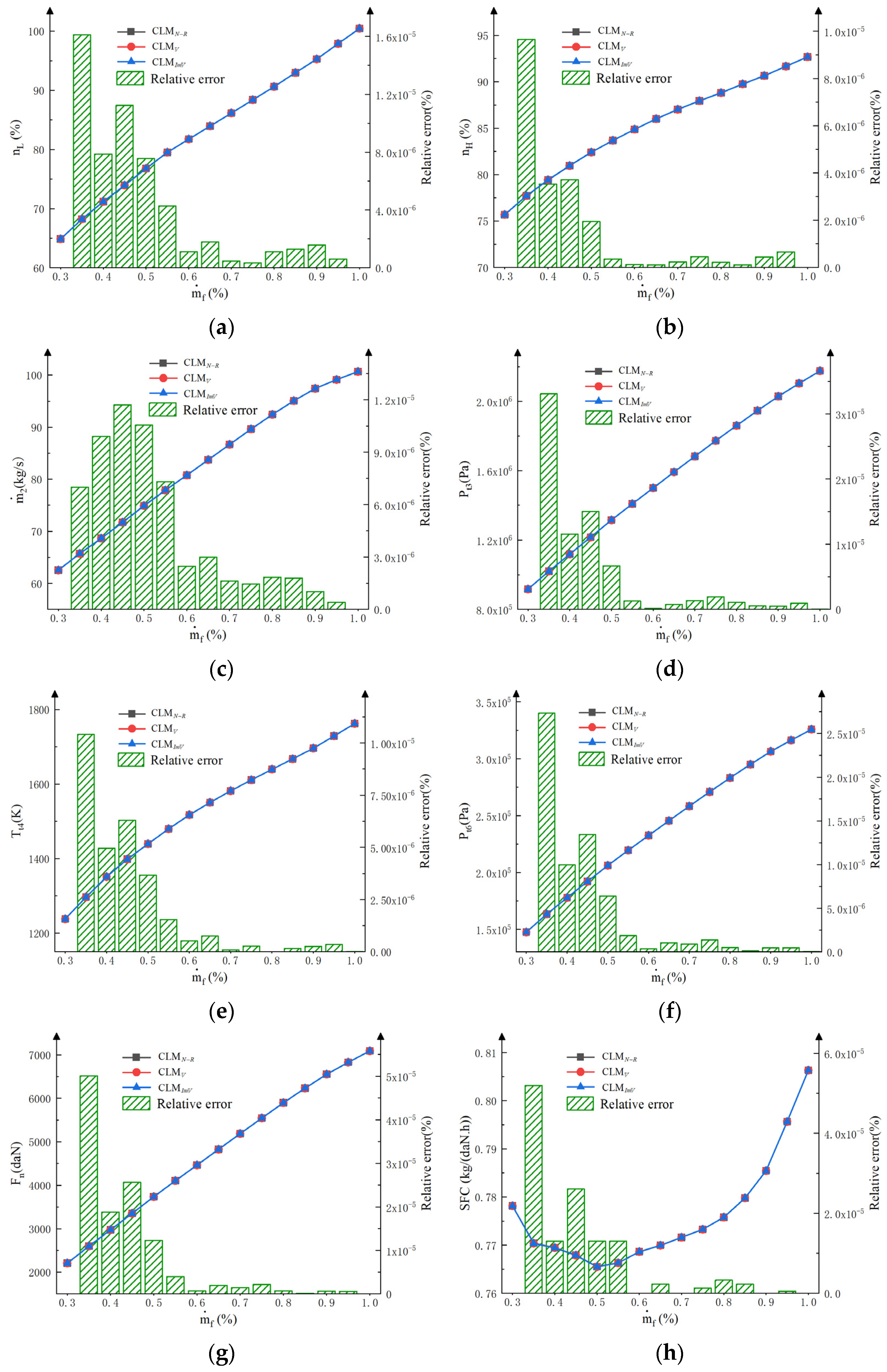
4.1. Comparison of Steady State

In order to verify the reliability of the variable cycle engines established in this paper, the performance calculation results of the model under two working modes were compared with the test data from foreign public sources [36]. Under ground conditions, the total thrust of the engine is maintained constant through fuel control, and the specific fuel consumption (SFC) is calculated by adjusting the variable geometric parameters, as shown in Figure 7. Since the variable cycle engines studied in this paper and the engines in the literature have differences in geometric dimensions and design parameters, deviations inevitably exist in the final calculation results. Therefore, the focus of the comparison is not on the absolute numerical values but on the changing trends. Figure 7a and Figure 7b, respectively, show the influence of $A_8$ and $A_{LT}$ on the changing trend of the fuel consumption rate.

The comparison in Figure 7 shows that under ground conditions, the changing trend of the fuel consumption rate of the steady-state performance matching model is basically consistent with the test data in the NASA report. A further comparison is made of the relationship between the engine’s relative inlet flow rate, total thrust, and specific fuel consumption, as shown in Figure 8.

In Figure 8a, the engine is in subsonic cruise mode, with fuel control maintained to keep the total thrust constant, and the inlet air flow of the engine is regulated to compare the impact on the variation trend of the fuel consumption rate. Figure 8b shows the variation trend of specific fuel consumption with total thrust under the two operating modes. As can be seen from Figure 8, the variation trend of specific fuel consumption of the performance matching model with inlet flow and total thrust is consistent with the test data.

To verify the computational accuracy of the established volumetric dynamics model, the steady-state errors are compared with those of the Newton–Raphson iteration model. Under international standard atmospheric conditions at sea level, keeping other control parameters constant, the fuel flow rate in the main combustion chamber is varied from 30% to 100% of the design point, with intervals of 5%. Simulation results for 15 steady-state operating points are shown in Figure 9. The horizontal axis represents the fuel flow rate of the main combustion chamber, and the vertical axis represents the key performance and state parameters of the VCE. The bar chart shows the relative error between the improved volumetric dynamics model ${\mathrm{CLM}}_{Im𝕍}$ and the iteration-based model ${\mathrm{CLM}}_{N-R}$.

As shown in Figure 9, when giving the same input, the Newton–Raphson iteration model, conventional volumetric dynamics model, and improved volumetric dynamics model exhibit remarkably similar output results for each steady-state point. The maximum relative error is only 0.0052%. This demonstrates that the improved volume dynamics model established in this study achieves a high degree of steady-state accuracy. To further analyze the accuracy and computational power, the root mean square error (RMSE) of each steady-state process is compared in Figure 9, in which the accuracy comparison is based on the iterative model; the results are shown in

Table 1. Table of comparison for accuracy.

Model	${\mathit{n}}_{\mathit{L}}$ RMSE	${\mathit{n}}_{\mathit{H}}$ RMSE	${\dot{\mathit{m}}}_2$ RMSE	${\mathit{T}}_{\mathit{t}4}$ RMSE	${\mathit{P}}_{\mathit{t}6}$ RMSE
${\mathrm{CLM}}_{𝕍}$	0.0035%	0.0034%	0.0041%	0.0029%	0.0025%
${\mathrm{CLM}}_{Im𝕍}$	0.0034%	0.0034%	0.0040%	0.0029%	0.0018%

.

As can be seen in Table 1, the traditional volumetric dynamics model and the improved volumetric dynamics model have little difference in their root mean square error, except for pressure. The improved volumetric dynamics model takes into account the constraint condition of the static pressure balance in the mixer like the iterative model, so the root mean square error is significantly reduced.

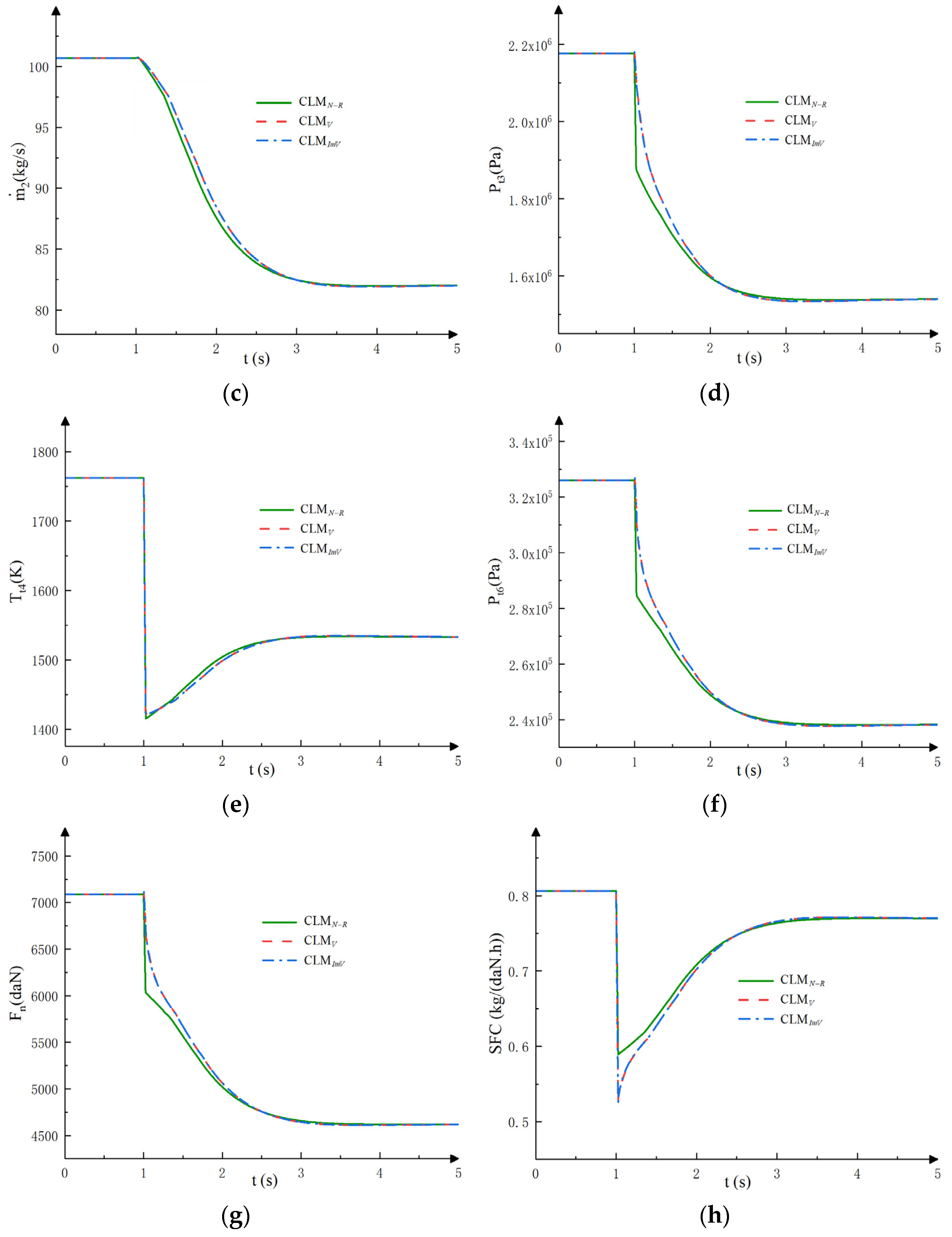
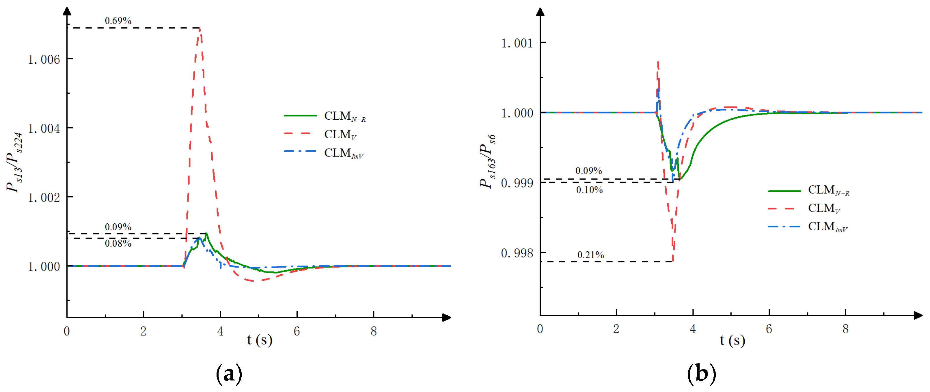
4.2. Comparison of Transition State

To further validate the dynamic accuracy of the improved volumetric dynamic model, a comparison of the transient state simulation results is conducted. To facilitate a more effective comparison of the dynamic simulation results among the three models and demonstrate the advantage of the volume-based model in maintaining smooth transitions under abrupt changes, the simulation conditions are set with standard atmospheric conditions at sea level, where the fuel flow rate linearly decreases from 1.588 kg/s to 0.988 kg/s within 25 ms; starting at 1 s, the results are shown in Figure 10.

As shown in Figure 10, the quasi-steady-state points of the iteration method model and the volumetric dynamic model are essentially the same, but their dynamic behaviors differ. During the dynamic variations of the HPC outlet pressure $P_{t3}$, LPT outlet pressure $P_{t6}$, and thrust $F_n$, the volumetric dynamic model exhibits a significantly smoother response compared to the iteration method model. The sudden decrease in the fuel flow rate in the combustion chamber causes a sharp change in the specific fuel consumption $SFC$, and since the volume model is more sensitive to flow rate variations, it is reasonable that the simulation curve of $SFC$ for the volume based model shows greater fluctuations compared to the iteration method model. The single-step simulation time of the dynamic process shown in Figure 10 is compared, and the results are shown in

Table 2. Table of comparison for single-step simulation time.

Model	Average Time of Single-Step	Total Time
${\mathrm{CLM}}_{N-R}$	0.269 ms	2.34 ms
${\mathrm{CLM}}_{𝕍}$	0.105 ms	3.65 ms
${\mathrm{CLM}}_{Im𝕍}$	0.103 ms	2.35 ms

.

As can be seen from Table 2, the iterative model requires multiple flow path calculations, so the single-step simulation time is larger. The volume dynamics model only carries out a single flow path calculation, so the single-step simulation takes less time. However, from the analysis of the total simulation time, the iterative model can converge quickly in the dynamic process, requiring fewer simulations, and the total simulation time required for convergence is only 2.34 ms. The number of simulations required for the convergence volumetric model is more and the total simulation time is larger. Due to the selection of an appropriate simulation step size and volume size, the total simulation time of the improved volumetric dynamics model is significantly reduced. To further compare the transition state between models, the fan co-operating line of this transient process is shown in Figure 11.

As shown in Figure 11, the fan co-operating lines of iteration method model and the volumetric dynamic model nearly coincide under steady-state conditions. During the transient state process, the iteration method model exhibits a sudden drop and sharp turns, which are inconsistent with the actual physical behavior of the engine. This phenomenon corresponds to the abrupt changes observed in $P_{t3}$, $P_{t6}$, and $F_n$ in Figure 10. In contrast, the co-operating line of the volumetric dynamic model varies smoothly, aligning better with the actual operational trends of the engine.

This clearly shows the difference between the iterative method model and the volumetric dynamics model. The iteration method model does not consider the engine’s real physical conditions during transient state processes, but instead only balances the co-operating equations in a faster way. Additionally, the volumetric dynamic model can reflect the characteristics of transient state processes more accurately, and the simulation results are closer to the real situation in the case of a sudden change. In terms of real-time performance, the iterative method model demonstrates advantages, whereas regarding dynamic characteristics, the volumetric method model exhibits superior capabilities.

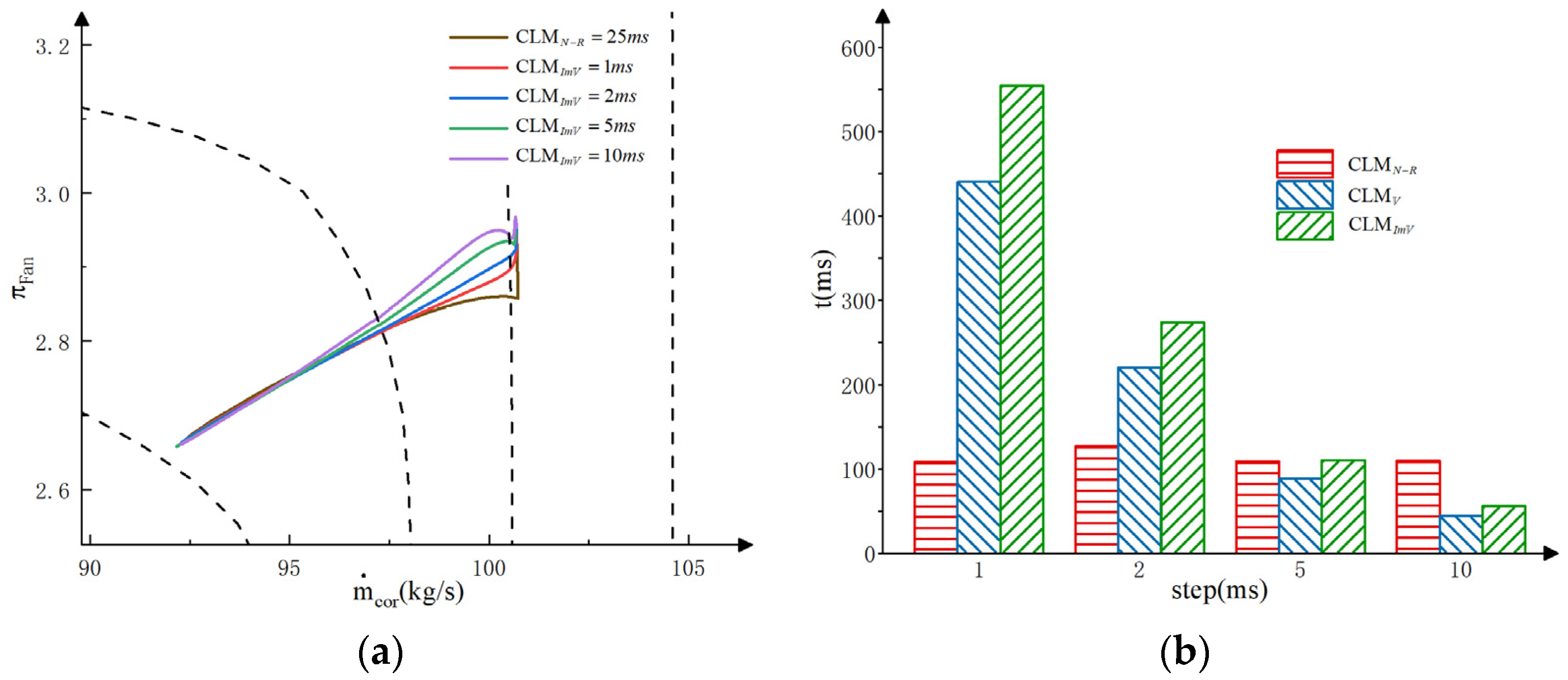
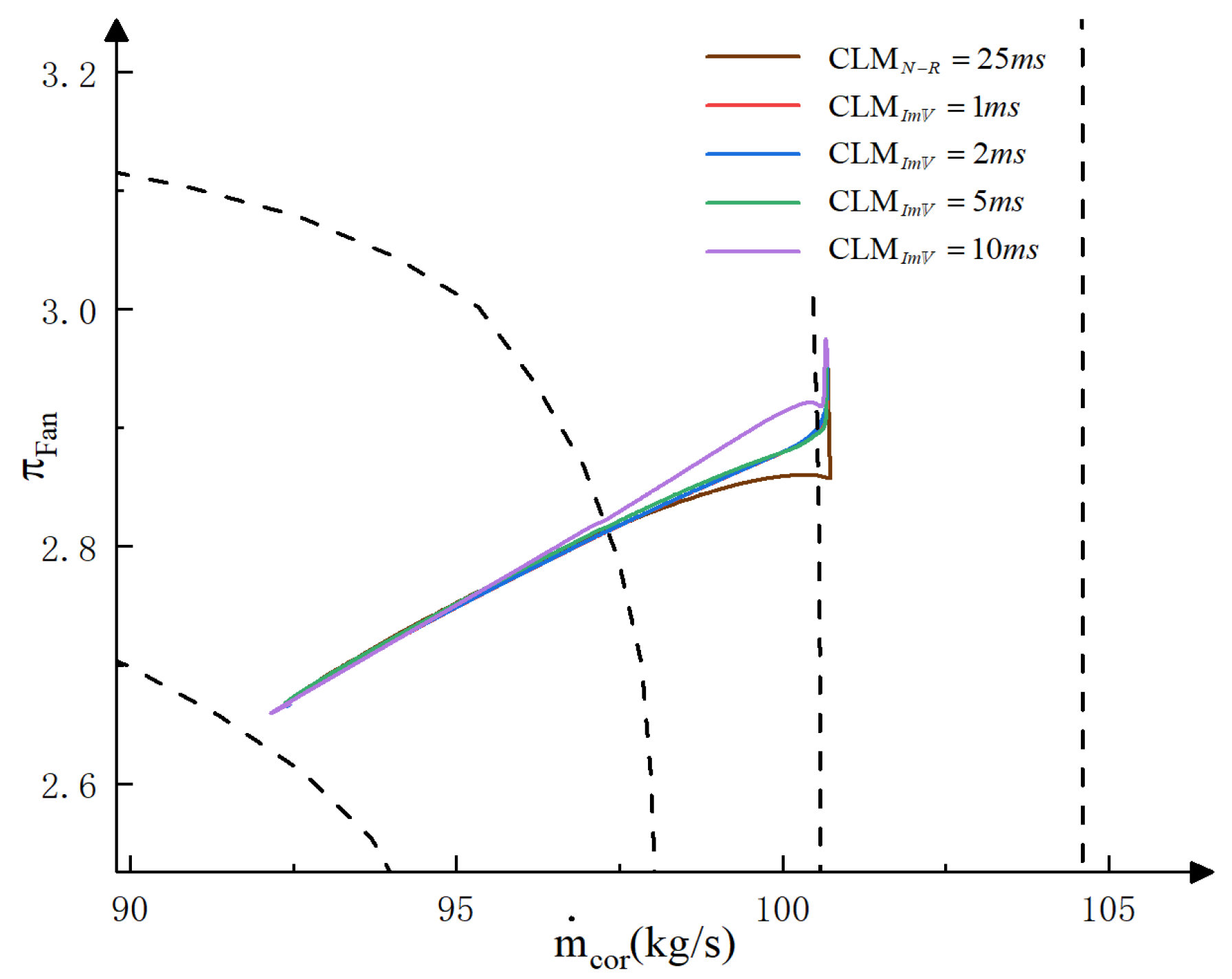
4.3. Simulation of Improved Volumetric Dynamics Model

This study integrates the pressure ratio collaborative update method and the adaptive virtual volume method to propose an improved volumetric dynamics modeling approach. This section provides a detailed description of the simulation results based on the improved method. To verify the effectiveness of the pressure ratio collaborative update method, the set VCE is operating in double-bypass mode under standard atmospheric conditions at sea level, with other control parameters constant. The fuel flow rate increases linearly from 1.2 kg/s to 1.588 kg/s starting at 3 s, with an increase in time of 0.5 s. The variations of the static pressure at the front and rear mixer inlet are compared, as shown in Figure 12.

As shown in Figure 12, for the Newton–Raphson iteration model, conventional volumetric dynamics model, and improved volumetric dynamics model, the maximum change rate of static pressure at the front mixer inlet is 0.09%, 0.69%, and 0.08%, respectively, while the maximum change rate at the rear mixer inlet is 0.09%, 0.21%, and 0.10%. The maximum static pressure change rates of both the iteration method model and the improved volumetric dynamics model are no greater than 0.10%, which is significantly smaller compared to the conventional volumetric dynamics model. This demonstrates that the improved method, which incorporates the pressure ratio collaborative update, can overcome the limitations of the conventional volume method by accounting for the static pressure balance constraint at the mixers. As a result, the model can better reflect the actual dynamic physical processes.

To verify the effectiveness of the proposed adaptive virtual volume method, under the same operating conditions and input as Figure 5a, the benchmark model is selected based on the smoothness of the co-operating line when the simulation time step is set to 1 ms. The initial virtual volume size and the optimal virtual volume sizes obtained through PSO for different simulation time steps are shown in

Table 3. Table of virtual volume size under different simulation steps.

Step	${𝕍}_{\mathit{I}}$/m3	${𝕍}_{\mathit{I}\mathit{I}}$/m3	${𝕍}_{\mathit{I}\mathit{I}\mathit{I}}$/m3	${𝕍}_{\mathit{I}\mathit{V}}$/m3	${𝕍}_{\mathit{V}}$/m3	t/ms	$\mathit{J}$
1 ms	1	2	2	2	3	554.4	5.0000
2 ms	5.50	1.01	1.94	9.70	3.07	273.6	4.9999
5 ms	7.77	0.27	13.52	11.64	1.96	110.1	4.9995
10 ms	12.82	0.45	7.67	14.10	1.95	55.8	4.9977

. The improvement of the fan co-operating line after using the optimal virtual volume is shown in Figure 13.

As shown in Figure 13, the fan co-operating lines for simulation time steps of 1 ms, 2 ms, and 5 ms almost overlap, with no noticeable deviation from the reference operating line as the simulation step increases, which is observed in Figure 5a. For a simulation time step of 10 ms, although adjusting the virtual volume does not fully achieve the optimal state, there is still a noticeable improvement. To further investigate the impact of the virtual volume size on the dynamic process, the variations in rotor speed before and after adjusting the virtual volume under the aforementioned simulation conditions are shown in Figure 14.

As shown in Figure 14a, before adjusting the virtual volume, the dynamic variation in rotor speed gradually exhibits a lagging phenomenon as the simulation time step increases. This is caused by the enhanced volume effect resulting from the larger simulation time step. However, as seen in Figure 14b, with the optimal virtual volume size, the lag effect in rotor speed dynamic variation is significantly reduced. This further demonstrates that adjusting the virtual volume size can mitigate the dynamic characteristic lag caused by an increase in the simulation time step.

From the perspective of simulation real-time performance, a larger simulation time step is preferred, but from the perspective of simulation accuracy, a smaller time step is desired. In practical application, the adaptive virtual volume method can select the optimal simulation step within the current volume by evaluating the deviation of the current co-operating line from the benchmark line. It comprehensively considers both real-time performance and calculation accuracy. The introduction of the adaptive virtual volume method reduces the lag effect caused by increasing the simulation time step, which improves the real-time performance of the volumetric dynamics model while ensuring the dynamic tracking capability.

5. Conclusions

This paper proposes an improved volumetric dynamics modeling method for the VCE based on the pressure ratio collaborative updating method and adaptive virtual volume method. According to the obtained results, the following conclusions can be drawn:

(1)

Based on the systematic analysis of the volumetric dynamics modeling process and flow path updating mechanism, a complex configuration model of the VCE is established.

(2)

A pressure ratio collaborative update method is proposed to address the oversight of the static pressure balance constraint at the mixer in conventional volumetric models. This method also offers a more accurate simulation of the nozzle’s impact on engine dynamic performance matching.

(3)

An adaptive virtual volume method is proposed by using cosine similarity as the optimization criterion. This method improves the model’s real-time performance while preserving the dynamic advantages of the volumetric dynamic method.

(4)

The steady-state error of volumetric dynamics model is no greater than 0.0052%, and the transient state simulation curves are smoother, which means the model can capture the actual physical characteristics of VCE more accurately.

It is worth mentioning that this paper establishes component-level models for the VCE based on both the volumetric dynamics method and the iteration method. A comparison is made to indicate the strengths and weaknesses of the two modeling methods in detail, which is significantly important for the development of aero-engine component-level modeling techniques.

The proposed improved volumetric dynamics modeling method is mainly applied to the component-level modeling of aero-engines. In the future, we will combine the improved volume dynamics model proposed in this paper with machine learning methods to further explore a more advantageous hybrid model modeling method.

References

1. Aygun, H.; Turan, O. Exergetic sustainability off-design analysis of variable-cycle aero-engine in various bypass modes. Energy 2020, 195, 117008. [Google Scholar]
2. Jia, X.; Zhou, D.; Wei, X.; Wang, H. A novel performance analysis framework for adaptive cycle engine variable geometry components based on topological sorting with rules. Aerosp. Sci. Technol. 2023, 141, 108579. [Google Scholar]
3. Jia, X.; Zhou, D. Multi-variable anti-disturbance controller with state-dependent switching law for adaptive cycle engine. Energy 2024, 288, 129845. [Google Scholar] [CrossRef]
4. Tahan, M.; Tsoutsanis, E.; Muhammad, M.; Karim, Z.A. Performance-based health monitoring, diagnostics and prognostics for condition-based maintenance of gas turbines: A review. Appl. Energy 2017, 198, 122–144. [Google Scholar] [CrossRef]
5. Zhang, X.; Zhang, T.; Sheng, H. A novel aeroengine real-time model for active stability control: Compressor instabilities integration. Aerosp. Sci. Technol. 2024, 145, 108844. [Google Scholar] [CrossRef]
6. Sheng, H.; Liu, T.; Zhao, Y.; Chen, Q.; Yin, B.; Huang, R. New model-based method for aero-engine turbine blade tip clearance measurement. Chin. J. Aeronaut. 2023, 36, 128–147. [Google Scholar] [CrossRef]
7. Wei, Z.; Zhang, S.; Jafari, S.; Nikolaidis, T. Gas turbine aero-engines real time on-board modelling: A review, research challenges, and exploring the future. Prog. Aerosp. Sci. 2020, 121, 100693. [Google Scholar]
8. Chen, J.; Hu, Z.; Wang, J. Aero-engine real-time models and their applications. Math. Probl. Eng. 2021, 2021, 9917523. [Google Scholar]
9. Aliramezani, M.; Koch, C.R.; Shahbakhti, M. Modeling, diagnostics, optimization, and control of internal combustion engines via modern machine learning techniques: A review and future directions. Prog. Energy Combust. Sci. 2022, 88, 100967. [Google Scholar]
10. Wang, J. Identification-based aeroengine nonlinear modeling: A comparative study. Simulation 2020, 96, 199–206. [Google Scholar]
11. Villarreal-Valderrama, F.; Liceaga-Castro, E.; Hernandez-Alcantara, D.; Santana-Delgado, C.; Ekici, S.; Amezquita-Brooks, L. Control-Oriented System Identification of Turbojet Dynamics. Aerospace 2024, 11, 630. [Google Scholar] [CrossRef]
12. Ma, Y.; Du, X.; Sun, X. Adaptive modification of turbofan engine nonlinear model based on LSTM neural networks and hybrid optimization method. Chin. J. Aeronaut. 2022, 35, 314–332. [Google Scholar] [CrossRef]
13. Wang, Y.; Huang, J.; Zhou, W.; Lu, F.; Xu, W. Neural network-based model predictive control with fuzzy-SQP optimization for direct thrust control of turbofan engine. Chin. J. Aeronaut. 2022, 35, 59–71. [Google Scholar] [CrossRef]
14. Ren, L.-H.; Ye, Z.-F.; Zhao, Y.-P. A modeling method for aero-engine by combining stochastic gradient descent with support vector regression. Aerosp. Sci. Technol. 2020, 99, 105775. [Google Scholar] [CrossRef]
15. Quevedo-Reina, R.; Álamo, G.M.; Padrón, L.A.; Aznárez, J.J. Surrogate model based on ANN for the evaluation of the fundamental frequency of offshore wind turbines supported on jackets. Comput. Struct. 2023, 274, 106917. [Google Scholar] [CrossRef]
16. Luo, X.; Geng, J.; Li, M.; Liu, B.; Wang, L.; Song, Z. Research on Iterative Calculation and Optimization Methods of Aero-engine On-board Model. J. Syst. Simul. 2022, 34, 2649–2658. [Google Scholar]
17. Pang, S.; Li, Q.; Feng, H. A hybrid onboard adaptive model for aero-engine parameter prediction. Aerosp. Sci. Technol. 2020, 105, 105951. [Google Scholar] [CrossRef]
18. Cheng, X.; Zheng, H.; Yang, Q.; Zheng, P.; Dong, W. Surrogate model-based real-time gas path fault diagnosis for gas turbines under transient conditions. Energy 2023, 278, 127944. [Google Scholar] [CrossRef]
19. Cai, W.; Zhao, Y.-P.; Zhu, Y.; Yin, J.; Xu, Z.-Y.; Liu, W.-M. A Novel Hybrid Aeroengine Modeling Method for Combining Data-Driven Modules. J. Aerosp. Eng. 2024, 37, 04024055. [Google Scholar] [CrossRef]
20. Wang, B.; Xuan, Y. Heuristic deepening of aero engine performance analysis model based on thermodynamic principle of variable mass system. Energy 2024, 306, 132481. [Google Scholar] [CrossRef]
21. Ozdemir, U. Comparison of the Newton–Raphson Method and genetic algorithm solutions for nonlinear aircraft trim analysis. Proc. Inst. Mech. Eng. Part G J. Aerosp. Eng. 2023, 237, 725–740. [Google Scholar]
22. Kong, X.; Wang, X.; Tan, D.; He, A. A non-iterative aeroengine model based on volume effect. In Proceedings of the AIAA Modeling and Simulation Technologies Conference, Portland, OR, USA, 8–11 August 2011; p. 6623. [Google Scholar]
23. Jia, Z.; Tang, H.; Jin, D.; Xiao, Y.; Chen, M.; Li, S.; Liu, X. Research on the volume-based fully coupled method of the multi-fidelity engine simulation. Aerosp. Sci. Technol. 2022, 123, 107429. [Google Scholar]
24. Palman, M.; Leizeronok, B.; Cukurel, B. Comparative study of numerical approaches to adaptive gas turbine cycle analysis. Int. J. Turbo Jet-Engines 2023, 40, 425–436. [Google Scholar]
25. Zheng, Q.; Li, L.; Zhang, H.; Chen, J. Research on a high-precision real-time improvement method for aero-engine component-level model. Int. J. Turbo Jet-Engines 2024, 41, 293–305. [Google Scholar]
26. Pang, S.; Li, Q.; Zhang, H. A new online modelling method for aircraft engine state space model. Chin. J. Aeronaut. 2020, 33, 1756–1773. [Google Scholar]
27. Fawke, A.J.; Saravanamuttoo, H.I.H. Digital computer methods for prediction of gas turbine dynamic response. SAE Trans. 1971, 80, 1805–1813. [Google Scholar]
28. Roberts, R.A.; Eastbourn, S.M. Modeling techniques for a computational efficient dynamic turbofan engine model. Int. J. Aerosp. Eng. 2014, 2014, 283479. [Google Scholar]
29. Yepifanov, S.; Zelenskyi, R.; Sirenko, F.; Loboda, I. Simulation of pneumatic volumes for a gas turbine transient state analysis. Turbo Expo: Power for Land, Sea, and Air. Am. Soc. Mech. Eng. 2017, 50916, V006T05A037. [Google Scholar]
30. Kurosaki, M.; Sasamoto, M.; Asaka, K.; Nakamura, K.; Kakiuchi, D. An efficient transient simulation method for a volume dynamics model. Turbo expo: Power for land, sea, and air. Am. Soc. Mech. Eng. 2018, 51128, V006T05A008. [Google Scholar]
31. Liu, Y.; Chen, M.; Tang, H. A versatile volume-based modeling technique of distributed local quadratic convergence for aeroengines. Propuls. Power Res. 2024, 13, 46–63. [Google Scholar]
32. Guo, C.; Sun, Y.; Li, L.; Zhu, X. High-Fidelity Simulation and Performance Analysis of Twin-Spool Turbofan Engine Based on Multi-dynamics Approach. Int. J. Aeronaut. Space Sci. 2024, 25, 1243–1256. [Google Scholar]
33. Pan, M.X.; Chen, Q.L.; Zhou, Y.Q.; Zhou, W.; Huang, J. A multi-dynamics approach to turbofan engine modeling. Chin. J. Aeronaut 2019, 40, 99–110. [Google Scholar]
34. Cai, C.; Zheng, Q.; Zhang, H. A new method to improve the real-time performance of aero-engine component level model. Int. J. Turbo Jet-Engines 2023, 40, 101–109. [Google Scholar]
35. Hashmi, M.B.; Lemma, T.A.; Ahsan, S.; Rahman, S. Transient behavior in variable geometry industrial gas turbines: A comprehensive overview of pertinent modeling techniques. Entropy 2021, 23, 250. [Google Scholar] [CrossRef]
36. French, M.; Allen, C. NASA VCE Test Bed Engine Aerodynamic Performance Characteristics and Test Results; AIAA Paper 1981–1594; NACA: Boston, MA, USA, 1981.
Figure 1. Architecture of variable cycle engine.
Aerospace 12 00274 g001
Figure 2. Main combustion chamber model schematic diagram.
Aerospace 12 00274 g002
Figure 3. VCE flow path calculation schematic diagram.
Aerospace 12 00274 g003
Figure 4. Pressure ratio collaborative updating schematic diagram.
Aerospace 12 00274 g004
Figure 5. Comparison between iterative method and volumetric method in modeling. (a) Fan co-operating lines. (b) Computational time.
Aerospace 12 00274 g005
Figure 6. Selection rules of vector angle for co-operating line schematic diagram.
Aerospace 12 00274 g006
Figure 7. Comparison of NASA report and volumetric dynamic models in variable geometric parameters. (a) The influence of A 8 . (b) The influence of A L T .
Aerospace 12 00274 g007
Figure 8. Comparison of NASA report and volumetric dynamic models in performance parameters. (a) Relative inlet flow rate of the engine. (b) Total thrust.
Aerospace 12 00274 g008
Figure 9. Comparison of steady state between iterative model and volumetric dynamic model. (a) Low-pressure shaft rotor speed n L . (b) High-pressure shaft rotor speed n H . (c) Fan inlet air flow rate m ˙ 2 . (d) HPC outlet total pressure P t 3 . (e) Combustion chamber outlet total temperature T t 4 . (f) LPT outlet total pressure P t 6 . (g) Thrust F n . (h) Specific fuel consumption S F C .
Aerospace 12 00274 g009
Figure 10. Comparison of transition performance simulation results between iterative model and volumetric dynamic model. (a) Low-pressure shaft rotor speed n L . (b) High-pressure shaft rotor speed n H . (c) Fan inlet air flow rate m ˙ 2 . (d) HPC outlet total pressure P t 3 . (e) Combustion chamber outlet total temperature T t 4 . (f) LPT outlet total pressure P t 6 . (g) Thrust F n . (h) Specific fuel consumption S F C .
Aerospace 12 00274 g010aAerospace 12 00274 g010b
Figure 11. Comparison of fan co-operating line for iterative model and volumetric model.
Aerospace 12 00274 g011
Figure 12. Comparison of static pressure simulation results of mixer. (a) Front mixer inlet static pressure ratio P s 13 / P s 224 . (b) Rear mixer inlet static pressure ratio P s 163 / P s 6 .
Aerospace 12 00274 g012
Figure 13. Fan co-operating line based on adaptive virtual volume method.
Aerospace 12 00274 g013
Figure 14. Comparison of rotor speed variation based on adaptive virtual volume method. (a) Before virtual volume adjustment. (b) After virtual volume adjustment.
Aerospace 12 00274 g014