Design of an Orbital Infrastructure to Guarantee Continuous Communication to the Lunar South Pole Region

Abstract

The lunar south pole has gained significant attention due to its unique scientific value and potential for supporting future human exploration. Its potential water ice reservoirs and favourable conditions for long-term habitation make it a strategic target for upcoming space missions. This has led to a continuous increase in missions towards the Moon thanks mainly to the boost provided by NASA’s Artemis programme. This study focuses on designing a satellite constellation to provide communication coverage for the lunar south pole. Among the various cislunar orbits analysed, the halo orbit families near Earth–Moon Lagrangian points L1 and L2 emerged as the most suitable ones for ensuring continuous communication while minimising the number of satellites required. These orbits, first described by Farquhar in 1966, allow spacecraft to maintain constant communication with Earth due to their unique geometric properties. The candidate orbits were initially implemented in MATLAB using the Circular Restricted Three-Body Problem (CR3BP) to analyse their main features such as stability, periodicity, and coverage time percentage. In order to develop a more detailed and realistic scenario, the obtained initial conditions were refined using a full ephemeris model, incorporating a ground station located near the Connecting Ridge Extension to evaluate communication performance depending on the minimum elevation angle of the antenna. Different multi-body constellations were propagated; however, the constellation consisting of three satellites around L2 and a single satellite around L1 turned out to be the one that best matches the coverage requirements.

1. Introduction

In recent years, the lunar south pole has attracted growing attention due to its remarkable scientific and strategic potential. With more than 140 missions planned between 2023 and 2033, the exploration of this region has become a priority for major space agencies worldwide [1,2]. This interest stems from both its unique geomorphological characteristics and the presence of permanently shadowed regions (PSRs), which are believed to contain significant deposits of water ice. These ice reservoirs, if confirmed, could serve as a crucial resource for future long-term lunar missions, providing essential support for a human presence by enabling in situ resource utilisation (ISRU) for drinking water, oxygen production, and fuel generation. Furthermore, certain elevated regions within the south pole receive near-continuous sunlight, making them ideal candidates for solar power installations that could sustain a permanent lunar base and other critical infrastructure [3].

The biggest effort arrives from NASA’s Artemis mission which aims to return humans to the Moon more than fifty years later. A key component of this effort is the Lunar Gateway, a space station planned to orbit the Moon, facilitating exploration missions and serving as a hub for scientific research and technology development. However, one of the primary challenges in establishing a sustainable lunar presence is ensuring continuous communication coverage over the south polar region. To address this, the European Space Agency (ESA) has introduced the Moonlight Initiative, a programme dedicated to developing a reliable lunar communication and navigation network that would provide uninterrupted connectivity between Earth, orbiting spacecraft, and surface missions [4]. To achieve continuous coverage of the lunar south pole, a multi-body constellation is essential. Various orbit options must be carefully analysed to determine the most effective configuration that balances coverage, stability, and operational cost. Various studies propose different orbital architectures that optimise communication and navigation for lunar exploration, pointing out that the stability of some elliptical orbits makes them highly cost-effective [5,6]; furthermore, ref. [6] evidences the excellent scalability of circular polar orbits united with their potential for global coverage even if they require a larger number of satellites. The study of cislunar dynamics, particularly leveraging orbits around Earth–Moon Lagrange points L1 and L2, presents a promising solution [7]. These orbits offer unique advantages in maintaining continuous communication with Earth due to their specific geometric properties. The first part of this work is aimed at selecting a family of orbits that would best verify the requirements for local continuous coverage of the lunar polar regions. Thereafter, the analysis provides new insights into the residence time of different satellite constellations over a specific Artemis’ landing site provided with different antenna minimum elevation angles; the constellations are propagated around Lagrangian points L1 and L2 exploiting high-fidelity simulations considering gravitational perturbations.

2. Multi-Body Constellation Design

The lunar gravitational environment is particularly complex, and simulations are not always straightforward, which is why different types of constellations are analysed in order to choose and develop the one that best suits the coverage requirements. One of the main drivers in the choice of orbits has been safeguarding the space around the lunar surface; developing a constellation system is crucial from the earliest stage of lunar exploration and colonisation, but it is crucial to do so in a responsible way and avoid unnecessarily overcrowding such a delicate near-surface environment, risking compromising the viability of the many future missions planned to our natural satellite.

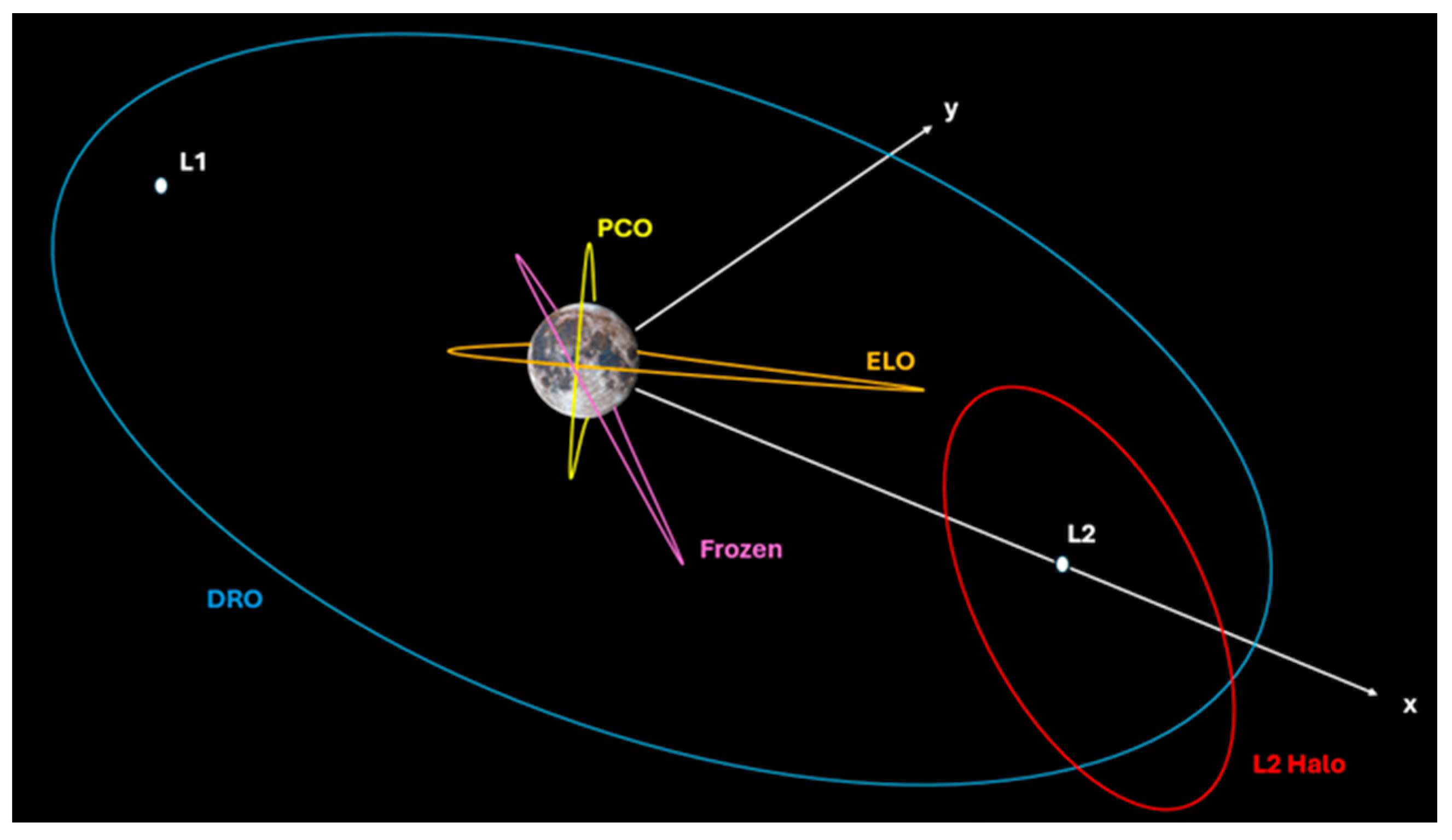
2.1. Possible Cislunar Orbits

There are several solutions for orbiting the Moon which will be presented below to provide an initial comparative assessment [8]; a visual representation is also provided in Figure 1.

• Low Lunar Orbits (LLOs) are typically circular orbits or slightly elliptical with an average altitude of around 100 km and any possible inclination; these orbits turn out to be the perfect candidate for surface access.
• Elliptical Lunar Orbits (ELOs) are equatorial orbits with a low perilune distance providing favourable access to the surface, but compared to the previous one they reduce access costs from Earth.
• Prograde Circular Orbits (PCOs) have a radius up to 5000 km; they are highly stable and require almost zero corrections to be maintained.
• Frozen Lunar Orbits are orbits with constant average eccentricity and an argument of periapsis values; this kind of orbit was discovered by analysing gravitational potential and looking for regions, corresponding to defined orbital parameters, in which effects due to perturbations are cancelled out or minimised. Those orbits exist for only certain combinations of energy, eccentricity, and inclination, and although they can provide high stability over time, research into them is not trivial. An in-depth study of this kind of orbit may be found in [9].
• Earth–Moon Liberation Point Halo Orbits are periodic orbits around the collinear liberation points which remain relatively fixed in the Earth–Moon plane, rotating at the same rate as that of the Moon around the Earth and that of the Moon around its own axis. Farquhar coined the term halo in 1966, noting how these orbits create a halo about the Moon by observing them from Earth [10]. Within a full ephemeris model, they may be slightly unstable, but their strengths include continuous Earth visibility, relatively easy access from Earth, and in certain cases predictable behaviour.
• Distant Retrograde Orbits (DROs) are a stable family of planar orbits about the smaller primary within the three-body problem [11].

In addition, a more detailed comparison of these orbits together with an assessment of their capability in Earth and lunar surface access as well as station-keeping cost and communication evaluations have been carried out in [8].

2.2. Lunar Constellation

Constellations of satellites have been increasingly used for the last 50 years for a wide variety of applications including global navigation systems, communication infrastructures, Earth observation, and many others. But while developments in “Earth Space” have made great strides by experimenting with ever more numerous and complex constellations, the same cannot be said for the lunar environment; lunar constellations are not a trivial issue and contrarily to Earth-orbiting constellations, lunar-distributed satellite systems are more expensive in deployment and maintenance.

A constellation around the Moon has never been established, but there have been a couple of missions that have included a formation flight in their operation scheduling: the Gravity Recovery and Interior Laboratory (GRAIL) and the Japanese Kaguya (SELENE) with two and three satellite formations, respectively [12,13]. Over the years, three distinct strategies have emerged as the leading approaches to constellation design; the first two are more historical and flight-proven while the third one was developed during the early years of the 21st century:

• The street-of-coverage design, typically involving satellites in polar orbits with a separation between the orbital planes selected such that the ground coverage of satellites in adjacent planes overlaps to provide full coverage.
• The Walker/Mozhaev constellation consisting of evenly distributed satellites in evenly distributed planes in circular orbits.
• The Flower Constellations (FCs) conceived by [14] based on placing all satellites on the same trajectory in a rotating reference frame. When viewed from the rotating frame, the common trajectory appears as multi-petaled “flowers”. An FC is generally characterised by repeatable ground tracks and suitable phasing mechanics. The basic requirements that an FC must have can be summarised as follows:

  -

  Identical orbit shape: anomalistic period, argument of perigee, height of perigee, and inclination;

  -

  Compatibility: the orbital period is evaluated in such a way as to yield a perfectly repeated ground track;

  -

  An equally displaced node line along the equatorial plane for each satellite in a complete FC.

Compared to the Walker constellation design, an FC design demonstrates higher performance given the higher number of possible design parameters [15]; furthermore, with the Flower Constellation the design process is generalised to include elliptical orbits allowing a greater focus on particular areas.

Architectures for Lunar South Pole Coverage

Useful guidelines to design a local coverage constellation are proposed in [16]; to provide redundant, continuous, and focused coverage minimising the number of satellites, orbits should have the following characteristics:

• Sufficiently large semi-major axis values to produce continuous single and double coverage with a minimal number of satellites;
• Large eccentricity values to focus coverage near apoapsis for longer contact durations;
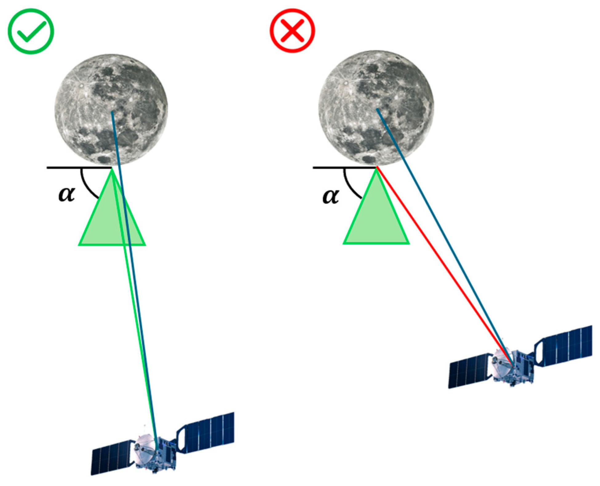
• Inclination values to orient the coverage swaths over the poles (rather than the equator);
• The argument of periapsis values set to either 90° or 270° depending on whether apoapsis should be over the south pole or north pole, respectively.

Having understood the necessary characteristics for a coverage constellation, the choice of the ideal orbit is the result of a thorough trade-off between the constellation stability, i.e., its lifetime, and the deploying and maintenance cost of the entire multi-body architecture, which is extremely tied to the number and size of the single spacecraft. For example, because of the Moon’s anisotropic gravitational field, the authors of ref. [17] have suggested a solution with an Elliptical Lunar Frozen Orbit (ELFO); ELFOs minimise sensitivity to external perturbations and provide persistent stable coverage to either the north or south pole with no requirements for station keeping for up to 10 years. However, given the proximity to the surface, insertion costs can increase exponentially. Even ref. [18] developed an LLO for small-sat constellation-exploiting areas of partial stability of the lunar environment, but their polar communication analysis makes use of over a hundred satellites; problems related to such numerous navigations and communication constellations have yet to be solved and may not be applicable. These include, for example, the proper design of efficient deployment schemes and the development of effective end-of-life disposal scenarios. Still, concerning the high number of orbiting satellites, a numerical analysis of the Flower Constellation provides its best performance, increasing the number of petals and consequently that of the orbiting spacecraft. Therefore, at least at this early exploratory stage, it might be prohibitive to push for such impactful solutions, risking compromising access to the lunar surface; furthermore, building a multi-body architecture in the immediate vicinity of the Moon requires larger beamwidths and/or constellation sizes to ensure horizon-to-horizon coverage [19]. After evaluating different possibilities to design a multi-body infrastructure, the Earth–Moon Lagrange points appear to be more viable locations to deploy these constellations.

2.3. Candidate Orbits: Halo Southern Families

The dynamical properties around the Lagrange points coupled with the fact that they have a large line of sight access area to the Moon’s surface make them a good candidate for deploying constellations with a minimal number of spacecraft [19]. Consequently, the southern families of halo orbits around collinear liberation points L1 and L2 could fit perfectly for this type of operation thanks to their prolonged permanence in the southern hemisphere of the Moon; for example, orbital mechanics analysis for the Lunar Gateway has selected L2 southern halo orbits, thereby demonstrating strong interest in this type of solution [20].

The most interesting subgroup of this family comprises Near-Rectilinear Halo Orbits (NRHOs). Within low-fidelity models, such as the three-body problem, NRHOs show favourable stability properties that suggest the potential to maintain their motion over a long duration while consuming few propellant resources; this can provide a good starting point for high-fidelity models. NRHOs offer advantages like relatively inexpensive transfer options from the Earth and feasible transfer options to the lunar surface and other orbits in cislunar space and beyond [21]. From a geometry point of view, they are distinguished by their elongated shape, a feature required for local coverage applications, and their constant visibility with selected ground stations on Earth’s surface. A spacecraft orbiting in an NRHO may be subject to the eclipsing of different durations and frequencies; it is therefore essential to control and predict this phenomenon. Orbital resonance is an important consideration for meeting eclipse constraints. Resonance in terms of the sidereal period is focused on the time required for a celestial body to complete a revolution in its orbit relative to another body (the Moon’s sidereal period is around 27.322 days); it corresponds to the period to see the Moon return to the same location in the sky from the centre of the Earth. On the other side, the synodic period is based on the time between the successive conjunctions of a celestial body with the Sun, and, in this case, it corresponds to the time to see the Moon return to the same location with respect to the Sun (the Moon’s synodic period is about 29.5306 days). Lastly, ref. [21] presented preliminary transfer studies demonstrating that NRHOs are accessible from Low Earth Orbits (LEOs) for a relatively low cost and short time of flight, which are crucial features for a crewed mission.

3. Dynamical Results

As a foundation for the design of a multi-body constellation, dynamical models with varying levels of fidelity have been employed. For the preliminary analysis, the Circular Restricted Three-Body Problem (CR3BP) has been implemented in MATLAB (R2023a) [22] (Figure 2a), providing a reliable approximation of the Earth–Moon system dynamics and enabling a deeper understanding of the behaviour of the selected orbital mechanics. This low-fidelity analysis yields the initial state vectors of the candidate orbits, which subsequently serve as the input for high-fidelity simulations. The need to introduce high fidelity is related to the fact that in reality corrective manoeuvres are required to ensure the periodicity of orbits. These simulations, conducted using GMAT and FreeFlyer [23,24], incorporate a full ephemeris model, accounting for the Moon’s gravitational field up to the 50th harmonic, as well as the perturbative influences of the Earth, the Sun, Jupiter, and solar radiation pressure (SRP). The high-fidelity phase ultimately enables the construction of the final constellation and a comprehensive global coverage analysis.

3.1. The Circular Restricted Three-Body Problem

Two masses m₁ and m₂ move in the circular orbits of radius r₁₂ about their centre of mass just under the action of their mutual gravitation; the reference frame (Figure 3) used is comoving and non-inertial with the x-axis directed toward m₂ and the y-axis being in the orbital plane to which the z-axis is perpendicular. To complete the system, a third body of negligible mass m compared to the primary ones is introduced; it has no effect on the motion of the other two bodies.

For the purposes of numerical analysis in MATLAB, it is convenient to use a dimensionless system of units to express the equation of motion through the following steps:

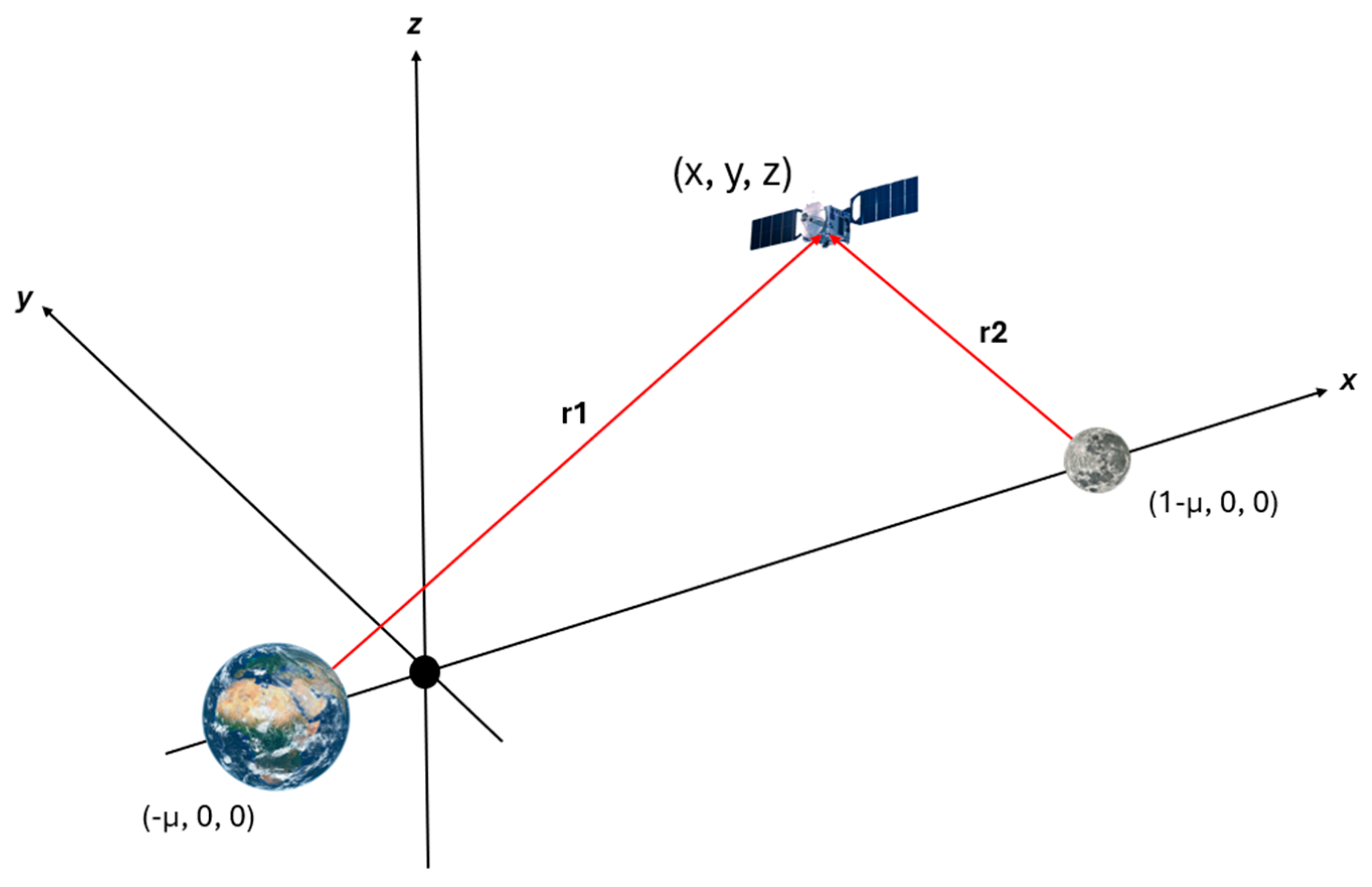
• The masses are normalised so that m₁ = 1 − µ and m₂ = µ, where µ = m₂/(m₁ + m₂) is the mass parameter of the system.
• The angular velocity of the comoving rotating frame is normalised to one.
• The distance between m₁ and m₂ has their coordinates in the reference system as (−µ, 0, 0) and (1 − µ, 0, 0) on the x-axis, as viewable in Figure 3. In this way, the distances of the third body to m₁ and m₂ are given by the following:

  $${\mathit{r}}_{\mathbf{1}}^{\mathbf{2}}={\left(\mathit{x}+\mathsf{\mu }\right)}^{\mathbf{2}}+{\mathit{y}}^{\mathbf{2}}+{\mathit{z}}^{\mathbf{2}}$$

  $${\mathit{r}}_{\mathbf{2}}^{\mathbf{2}}={\left(\mathit{x}-\mathbf{1}+\mathit{\mu }\right)}^{\mathbf{2}}+{\mathit{y}}^{\mathbf{2}}+{\mathit{z}}^{\mathbf{2}}$$
• Lastly, the introduction of the non-dimensional time τ is useful during the integration procedure

  $$\tau ={\displaystyle \frac{t}{t^{*}}}$$

  where t* is the characteristic time of the system

  $$t^{*}=\sqrt{{\displaystyle \frac{r_{12}^3}{G\left(m_1+m_2\right)}}}$$

  so the equations of motion expressed in a non-dimensional form become

  $$\ddot{x}-2\dot{y}=U_x$$

  $$\ddot{y}+2\dot{x}=U_y$$

  $$\ddot{z}=U_z$$

  thereby demonstrating the effective potential, and U_x, U_y and U_z are the partial derivatives of U with respect to the position variables.

  Table 1. Main characteristics of the Earth–Moon system useful for numeric implementation.

  Feature	Value
  Moon mass	7.3477 × 1022 [kg]
  Earth mass	5.97219 × 1024 [kg]
  µ [24]	0.0121505856
  Moon radius	1734.4 [km]
  Earth–Moon average distance (r12) [25]	385,000.6 [km]
  Characteristic time (t*)	4.3651274 [days]

  offers the main parameters of the Earth–Moon system.

The equations of motion can be associated with the following six-element state vector $\overrightarrow{\mathit{q}}$, which is defined as $\overrightarrow{\mathit{q}}={\left(\mathit{x} \mathit{y} \mathit{z} \dot{\mathit{x}}\dot{ \mathit{y}}\dot{ \mathit{z}}\right)}^{\mathit{T}}$. Then, the matrix of partial derivatives $\mathit{\delta }\overrightarrow{\mathit{q}}(\mathit{\tau }+{\mathit{\tau }}_{\mathbf{0}})/\mathit{\delta }\overrightarrow{\mathit{q}}\left({\mathit{\tau }}_{\mathbf{0}}\right)$, called the state transition matrix (STM), can be expressed as

$$\dot{\mathbf{\Phi }}\left(\mathit{\tau }+{\mathit{\tau }}_{\mathbf{0}},{\mathit{\tau }}_{\mathbf{0}}\right)=\mathit{A}(\mathit{\tau })\mathbf{\Phi }(\mathit{\tau }+{\mathit{\tau }}_{\mathbf{0}},{\mathit{\tau }}_{\mathbf{0}})$$

Since the matrix A(τ) is evaluated along the reference solution, its values depend on the time and the specific trajectory being followed. For this reason, A(τ) is generally not constant when considering an arbitrary trajectory, as its elements are influenced by the local dynamics and the state of the system at each point along the path. However, if the reference is a periodic solution, then A(τ) is periodic as well. A is a 6 × 6 matrix which is divided into four submatrices, each 3 × 3

$$\mathit{A}\left(\mathit{\tau }\right)=\left[\begin{array}{cc}{\mathbf{0}}_{\mathbf{3}\times \mathbf{3}}& {\mathit{I}}_{\mathbf{3}\times \mathbf{3}}\\ {\mathit{U}}_{\mathit{X}\mathit{X}}& \mathbf{\Omega }\end{array}\right]$$

where 0_3×3 is a zero matrix, I_3×3 is the identity matrix, and

$$\mathbf{\Omega }=\left[\begin{array}{ccc}\mathbf{0}& \mathbf{2}& \mathbf{0}\\ -\mathbf{2}& \mathbf{0}& \mathbf{0}\\ \mathbf{0}& \mathbf{0}& \mathbf{0}\end{array}\right]$$

and

$${\mathit{U}}_{\mathit{X}\mathit{X}}=\left[\begin{array}{ccc}{\mathit{U}}_{\mathit{x}\mathit{x}}& {\mathit{U}}_{\mathit{x}\mathit{y}}& {\mathit{U}}_{\mathit{x}\mathit{z}}\\ {\mathit{U}}_{\mathit{y}\mathit{x}}& {\mathit{U}}_{\mathit{y}\mathit{y}}& {\mathit{U}}_{\mathit{y}\mathit{z}}\\ {\mathit{U}}_{\mathit{z}\mathit{x}}& {\mathit{U}}_{\mathit{z}\mathit{y}}& {\mathit{U}}_{\mathit{z}\mathit{z}}\end{array}\right]$$

is the symmetric matrix of the second partial derivatives of U with respect to x, y, z evaluated along the orbit.

The STM is a fundamental element in determining the main features of an orbit because it supplies valuable information regarding both the stability of the system and predictions for variations along the path; it is essentially a linear map and reflects the convergence or divergence of variations relative to a reference solution. In this way, the problem involves 42 first-order differential equations, which arise from the formulation of the dynamics in a six-dimensional state space. Specifically, 36 of these equations represent the partial derivatives of the state transition matrix with respect to the state variables, while the remaining 6 equations correspond to the equations of motion for the state vector. Despite the non-integrability of the equations of motion in closed form, Poincarè, in 1892, proved that an infinite variety of periodic orbits exist in the three-body problem [7]. Generally, the computation of periodic orbits is not trivial, and, hereafter, the focus will be on generating halo family orbits and understanding their behaviour; the numerical algorithm developed in MATLAB is based on [7,26,27,28] studies.

The initial state vector of a halo orbit is expressible as

$$\overrightarrow{{\mathit{q}}_{\mathbf{0}}}={\left({\mathit{x}}_{\mathbf{0}},\mathbf{0},{\mathit{z}}_{\mathbf{0}},\mathbf{0},\dot{{\mathit{y}}_{\mathbf{0}}},\mathbf{0}\right)}^{\mathit{T}}$$

which is perpendicular to the x-z plane. The solution is also symmetric with respect to the x-z plane, so the state vector at T/2 is

$$\overrightarrow{\mathit{q}}\left({\displaystyle \frac{\mathit{T}}{\mathbf{2}}}\right)={\left(\mathit{x},\mathbf{0},\mathit{z},\mathbf{0},\dot{\mathit{y}},\mathbf{0}\right)}^{\mathit{T}}$$

and this orbit is defined as periodic with period T. A halo orbit can be considered periodic if $\left|\dot{\mathit{x}}\right|$ and $\left|\dot{\mathit{z}}\right|<{\mathbf{10}}^{-\mathbf{8}}$ at T/2.

After introducing the concept of periodicity, another important aspect is evaluating the stability of the orbits. For a periodic orbit, the monodromy matrix is defined as the STM after one full period T, $\mathit{\varphi }\left(\mathit{T}+{\mathit{\tau }}_{\mathit{i}},{\mathit{\tau }}_{\mathit{i}}\right);$ this matrix has two characteristic properties [21]:

• The eigenvalues of the monodromy matrix always appear in reciprocal pairs.
• One pair of eigenvalues is always equal to unity due to the periodicity of the orbit and the existence of a family of such orbits with precisely periodic behaviour. The other two reciprocal pairs of eigenvalues (λ_i, 1/λ_i) are combined into a single metric for the purpose of describing the stability; it is therefore possible to introduce the stability index as

  $${\mathit{\nu }}_{\mathit{i}}={\displaystyle \frac{\mathbf{1}}{\mathbf{2}}}\left({\mathit{\lambda }}_{\mathit{i}}+{\displaystyle \frac{\mathbf{1}}{{\mathit{\lambda }}_{\mathit{i}}}}\right) \mathit{f}\mathit{o}\mathit{r} \mathit{i}=\mathbf{1,2}$$

If both the stability indices are less than one in the modulus, the orbit can be considered marginally stable in a linear sense; otherwise, it is unstable. In ref. [7], the authors showed how the NRHO region could be considered as a demarcation line for stability; moving towards the Lyapunov orbits, the stability indices mark a considerable upsurge, while towards the Moon they tend to deviate little from unity, making almost all of them eligible at first instance. Moreover, the L1 NRHO family shows only a single stability interval, while the L2 NRHO one has two intervals of stables orbits; Figure 4 and Figure 5 point out these characteristic ranges, correlating them with the perilune distance of the orbits.

3.1.1. Preliminary Results

The initial state vector generated by [7] provided a suitable starting point for the orbital propagation, but it was necessary to readjust some coordinates since some values relating to the main characteristics of the Earth–Moon system have been updated (Table 1). In addition, the initial conditions of further orbits within the stability intervals were added.

Appendix A summarises the initial dimensionless conditions for generating the halo orbit families in L1 and L2 and their respective period T; the highlighted values represent orbits that lie within the stability range. As can be noticed, the first row of each table has the peculiarity of having zero z-coordinates, and the orbit generated corresponds to the bifurcation with the Lyapunov family, which consists of a series of planar orbits lying in the x-y plane.

3.1.2. Orbit Selection

For the coverage analysis, the concept of coverage time percentage (CTP) has been followed. The CTP of a region refers to the time that the region is covered by a satellite divided by the total time of simulation or a reference time, in our case the orbital period; a region is continuously covered if the CTP equals 100% [30]. As an initial analysis, the south polar region is considered as the area between latitudes −60° and −90°. For example, a CTP value of 75% means that a satellite orbits above the south polar region for 75% of its orbital period; thus, the subsatellite point has a latitude component below the threshold value for 75% of the considered period.

The CTP evaluation has been conducted for the entire halo family and led to the selection of three orbits (

Table 2. Main orbital features of the three selected orbits from the preliminary design (low fidelity). Only the two highlighted are the subject of the high-fidelity analysis.

Orbit	${\mathit{x}}_0$	${\mathit{z}}_0$	$\dot{{\mathit{y}}_0}$	Period (days)	Sinodic Res.	Sidereal Res.	CTP [%]	Perilune Distance
L1	0.9246	−0.2180	0.1232	7.8781	3.75	3.48	80.31	3905.9
L2	1.0694	−0.20105	−0.1860	9.4966	3.11	2.88	42.32	13,798.6
L2	1.0634	−0.2003	−0.1770	9.1155	3.24	3.00	47.22	12,005.7

) as the result of a compromise between a sufficiently elongated shape tied to the CTP value, stability for proximity to the NRHO family, and avoiding lowering the orbit perilune overly (e.g., below 1000 km altitude); the first one is chosen for its excellent performance in coverage, the second one for belonging to the NRHO family, and the latter for its sidereal resonance equal to 3. The integer values of resonance result in a more stable orbital behaviour.

However, the high-fidelity model demonstrates how only the first and third are viable solutions because the NRHO tends to lose the correct phase angle between satellites with the developed mission sequence. Figure 6 highlights this problem; the apolune oscillations cause a variation in the orbital period of each satellite that after some time results in latitude overlaps and the loss of continuous coverage properties. This type of constellation demands corrective manoeuvres to adjust the phasing, which add to those needed to ensure stability, thus resulting in an overall increase in cost.

As can be seen from the CTP values in Table 2, a constellation of satellites with a precise initial true anomaly is required to ensure 24 h coverage. An example of two possible combinations of satellites that can theoretically ensure a 100% CTP is presented in Figure 7 by dividing the orbit into ten equidistant parts in time; clearly, the chosen orbit around L1 requires at least two satellites while the one around L2 requires at least three.

3.2. High-Fidelity Simulations

The Moon has a complex gravitational environment strongly linked to the geological history of our natural satellite; the more accurate the mathematical models, the more reliable and realistic the simulations will be. Once again, the importance of a thorough knowledge of the history and characteristics of the Moon is emphasised. Especially when the satellite is near to the perilune, it is crucial to account for a larger number of gravitational perturbations which are associated with different harmonic contributions. Conversely, at greater distances from the Moon, only a few gravitational harmonics are sufficient to ensure accurate results.

To accomplish this objective, GMAT provides the LP-165 lunar gravity model where spherical harmonics up to 50 degrees are considered, thus supporting the accepted heuristic that the accurate modelling of the lunar orbits requires retaining at least fifty coefficients in the Selene potential [31]. Moreover, the gravitational influence of the Sun, Earth, and Jupiter are regarded. At last, although its contribution is highly dependent on the size and geometry of the satellite, the solar radiation pressure (SRP) is also taken into account; as a preliminary analysis, the default value of the SRP area provided by GMAT equal to 1 m² has been adopted.

All the simulations have been run with a satellite of 425 kg in accordance with that of Queqiao, the relay satellite orbiting around the L2 point during the Chinese mission Chang’e 4 [32]. Meanwhile, the chosen initial epoch expressed in the UTC Gregorian format is 1 January 2025. The mission sequence (Figure 8) involves two corrective manoeuvres per orbit at the apolune and perilune, respectively, with a target to be reached at the next apsidal point; in particular, at the perilune, the speed components in x and z are required to be equal to zero, while at the apolune a constraint is also added to position coordinate z in order to not compromise the design phasing. As a general guideline, extra constraining of the final conditions to achieve this within a target sequence does not allow the problem to converge properly and greatly increases the computational cost. Moreover, without the aid of corrective manoeuvres, the orbits diverge after 4/5 days according to [7]. For this work, it has been decided to provide continuous thrust for the entire simulation time, for this lowers the required thrust levels and improves the overall trajectory control. In the first instance, simulations for all the different types of constellations provide thrust values that stand a few dozen mN, in line with the thrust produced by some types of electric propulsion, i.e., Hall effect thrusters.

3.2.1. Earth Visibility

As has previously emerged, one of the main features of certain halo orbits is their constant visibility from Earth; the stronger candidate Earth ground stations belong to the Deep Space Network (DSN). Communications through this system with lunar space have already been extensively tested; currently, the Korean Pathfinder Lunar Orbiter (KPLO) utilises the DSN’s facilities. The DSN is NASA’s international array of giant radio antennas that supports interplanetary spacecraft missions. It consists of three facilities spaced equidistant from each other (about 120 degrees apart in longitude). These sites are located in Goldstone (California), Madrid (Spain), and Canberra (Australia), as shown in Figure 9; their positions ensure that once a spacecraft sinks below the horizon at one DNS site, another facility can pick up the signal and carry on communicating. The FreeFlyer (version 7.8) software is well suited for the verification of this assumption; in its library, Freeflyer owns a series of custom Earth ground stations with their real horizon masks, among which there are also the DSN’s antennas. After the selected L1 and L2 orbits have been propagated using GMAT, the generated ephemeris is imported into FreeFlyer. By creating contact vectors between the spacecraft and the three DSN ground stations, it is possible to observe how there is always a facility in sight.

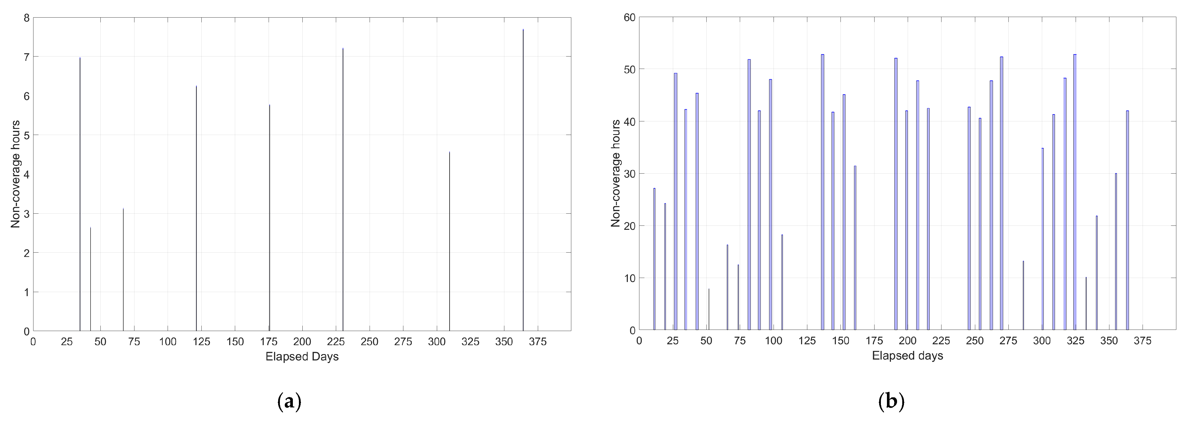
3.2.2. Constellation Design and Coverage Analysis

The objective of the following simulations is to assess how and through which design choices it is possible to guarantee 24 h lunar south pole coverage with at least one satellite in sight; in particular, for this analysis the time interval considered is equal to 365 days. As the preliminary coverage analysis within the CR3BP has already highlighted, a dedicated constellation with properly phase-shifted satellites is required.

In order to provide tangible data on coverage, it is necessary to introduce a ground station at the lunar south pole; in this work, the area defined as the Connecting Ridge Extension (Figure 10) due to its elevation and proximity to two interesting PSRs (Shackleton and De Gerlache) has been chosen for the placement of a communication facility. Its geodetic coordinates are 89.1° S and 110° W. In general, the proposed results can provide a good coverage indication also for the other regions of interest very close to the real south pole. The coverage performance is verified by correlating the minimum elevation angle of each antenna (the smallest angle above the horizon at which the antenna can effectively establish and maintain communication with a target) with the respective latitude of the satellite, as shown in

Table 3. Selected antenna minimum elevation angles compared to the spacecraft minimum associated latitude within the view cone.

Antenna Minimum Elevation Angle α [°]	Associated Latitude [°]
15	−18
20	−22
40	−42
60	−60

and Figure 11. This correlation is achieved by observing which are the equivalent latitudes of the satellite in and out of the cone of view of the antenna itself (through the FreeFlyer software); consequently, the considered latitude values become the thresholds used in the coverage analysis. Hence, a satellite is considered in sight if its latitude is lower than the threshold one.

The choice to cover such a wide range of values is dependent on the fact that there are no established values about the minimum elevation angles for a lunar ground station in the literature. Some Earth ground stations show elevation angles well below 10°, but, at least initially, it is not conceivable to do the same on the lunar surface. A more conservative approach has been preferred, which could also include rather stringent values to simulate more prohibitive locations, such as craters with particularly steep walls; this constitutes the rationale for also including antenna minimum elevation angles equal to 60°. Lastly, it is important to emphasise that this is a worst-case scenario which considers only the geodetic coordinates of the satellites for coverage purposes; surely, adding the possibility of having a steerable antenna on the satellite could greatly extend the coverage percentage.

Different combinations of constellations that should theoretically ensure total coverage have been evaluated, but the one that guarantees the best performance consists of three satellites in orbit L2 propagated, respectively, from positions 0, 4, 7 of Figure 7 and a satellite in L1 starting from the apolune, as can be seen in Figure 12. The combination of satellites both in orbit around L1 and around L2 allows us to ensure better regularity in coverage thanks to the greater elongation of the satellite trajectory in L1. With a minimum elevation angle of 60°, the annual non-coverage hours amount to approximately 44 h with a maximum non-coverage gap of 7.68 h, Figure 13. It is sufficient to decrease α by just one degree to guarantee a 100% CTP.

4. Discussion

The results from the previous section make it clear that the solution providing the best multi-body constellation design is the one with the three satellites on the 3:1 sidereal resonant L2 halo orbit and the one satellite propagated from the apolune on the L1 halo. Moreover, a value-added feature of this type of constellation is evident in Figure 14, where it is clearly visible how the time intervals in which the satellites on L2 decrease their latitude in magnitude are well compensated by the presence of the satellite in L1, ensuring better uniformity in coverage. The entire constellation has been propagated within the GMAT R2022a software by combining the ephemeris of each satellite, and Figure 15 provides an overall view from different reference frames. This work presents itself as a preliminary iteration analysis of the local coverage of the lunar south pole and in particular of the regions of interest within the Artemis programme; certainly, the future scheduled lunar missions will provide many of the answers that are currently missing, and they will help to improve the design processes of these ambitious programmes. Several adjustments can be made for future investigations which include the following:

• Improvement of the preliminary simulation within the CR3BP moving to a more detailed analysis exploiting the Bicircular Restricted Four-Body Problem (BCR4BP) which considers the solar influence; this could surely enhance the stability analysis and enrich the library of initial state vectors for orbits around the Lagrange point of the Earth–Moon system.
• Searching for combinations of orbits with periods as similar as possible to overcome the phase synchronisation issues observed in the previous sections. Ensuring the best possible phase control means minimising the need for corrective manoeuvres to restore the nominal conditions of the constellation, thus reducing costs.
• Refining the gravitational model within the high-fidelity simulations.
• Introducing a detailed satellite geometry such as the spacecraft surface area to conduct highly realistic assessments on station keeping and the propulsion system.
• Improvement of the communication analysis by equipping the satellite with a suitable antenna and introducing possible functional and performance requirements for the entire telecommunication infrastructure. Also, from a communication point of view, it will be interesting to provide an order of magnitude regarding the maximum tolerable coverage gaps for lunar ground facilities.
• Observing the contribution of the Gateway project and understanding if it could contribute to the telecom constellation.

5. Conclusions

This work proposes a possible orbital solution for the requirement to ensure continuous communication to the lunar south pole regions by demonstrating its feasibility through a properly designed constellation of halo orbits around Lagrange points L1 and L2. Furthermore, it can provide not only the crucial steps of the design flow of halo orbits but it may also be effectively generalised to other binary body systems as long as they satisfy the fundamental theoretical principles.

References

1. Cohen, B.A. Lunar Mission Priorities for the Decade 2023–2033; NASA: Washington, DC, USA, 2020. [Google Scholar]
2. Tai, W.; Cosby, M.; Lanucara, M. Lunar Communications Architecture Study Report (v1. 3). Interagency Operations Advisory Group, Lunar Communications Architecture Working Group. 2022. Available online: https://www.ioag.org/Public%20Documents/Lunar%20communications%20architecture%20study%20report%20FINAL%20v1.3.pdf (accessed on 14 February 2025).
3. Trabacchin, N.; Ochner, P.; Colombatti, G. A Physical and Spectroscopic Survey of the Lunar South Pole with the Galileo Telescope of the Asiago Astrophysical Observatory. Aerospace 2024, 11, 693. [Google Scholar] [CrossRef]
4. ESA Moonlight. Available online: https://connectivity.esa.int/esa-moonlight (accessed on 31 January 2025).
5. Ely, T.A. Coverage and Control of Constellations of Elliptical Inclined Frozen Lunar Orbits. In Proceedings of the 2005 AAS/AIAA Astrodynamics Specialist Conference, Lake Tahoe, CA, USA, 7–11 August 2005. [Google Scholar]
6. Lu, Y.; Yang, Y.; Li, X.; Zhu, Z.; Li, H.; Dong, G. Lunar Polar Orbit Relay Constellation and Its Deployment and Maintenance. In Proceedings of the 2012 Second International Conference on Intelligent System Design and Engineering Application, Sanya, China, 6–7 January 2012; pp. 333–336. [Google Scholar] [CrossRef]
7. Grebow, D. Generating Periodic Orbits in the Circular Restricted Three-Body Problem with Applications to Lunar South Pole Coverage. Master’s Thesis, School of Aeronautics and Astronautics, Purdue University, West Lafayette, IN, USA, 2006; pp. 8–14. [Google Scholar]
8. Whitley, R.; Martinez, R. Options for staging orbits in cislunar space. In Proceedings of the 2016 IEEE Aerospace Conference, Big Sky, MT, USA, 5–12 March 2016; pp. 1–9. [Google Scholar]
9. Cinelli, M.; Ortore, E.; Mengali, G.; Quarta, A.A.; Circi, C. Lunar orbits for telecommunication and navigation services. Astrodynamics 2024, 8, 209–220. [Google Scholar]
10. FARQUHAR, R.W. Lunar communications with libration-point satellites. J. Spacecr. Rocket. 1967, 4, 1383–1384. [Google Scholar] [CrossRef]
11. Hénon, M. Numerical exploration of the restricted problem, V. Astron. Astrophys. 1969, 1, 223–238. [Google Scholar]
12. GRAIL. Available online: https://www.jpl.nasa.gov/missions/gravity-recovery-and-interior-laboratory-grail/ (accessed on 31 January 2025).
13. SELENE (Selenological and Engineering Explorer). Available online: https://www.eoportal.org/satellite-missions/selene (accessed on 31 January 2025).
14. Mortari, D.; Wilkins, M.P.; Bruccoleri, C. The Flower Constellations. J. Astronaut. Sci. 2004, 52, 107–127. [Google Scholar] [CrossRef]
15. Mortari, D.; De Sanctis, M.; Lucente, M. Design of Flower Constellations for Telecom Munication Services. Proc. IEEE 2011, 99, 2008–2019. [Google Scholar] [CrossRef]
16. Ely, T.A. Stable constellations of frozen elliptical inclined lunar orbits. J. Astronaut. Sci. 2005, 53, 301–316. [Google Scholar] [CrossRef]
17. Ely, T.A.; Lieb, E. Constellations of elliptical inclined lunar orbits providing polar and global coverage. J. Astronaut. Sci. 2006, 54, 53–67. [Google Scholar] [CrossRef]
18. Shirobokov, M.; Tromov, S.; Ovchinnikov, M. Lunar Frozen Orbits for Small Satellite Communication/Navigation Constellations. In Proceedings of the International Astronautical Congress, IAC, Dubai, United Arab Emirates, 25–29 October 2021. [Google Scholar]
19. Nallapu, R.; Vance, L.D.; Xu, Y.; Thangavelatham, J. Automated design architecture for lunar constellations. In Proceedings of the 2020 IEEE Aerospace Conference, Big Sky, MT, USA, 7–14 March 2020; pp. 1–11. [Google Scholar]
20. Lee, D.E. White Paper: Gateway Destination Orbit Model: A Continuous 15 Year Nrho Reference Trajectory; No. JSC-E-DAA-TN72594; NASA: Washington, DC, USA, 2019. [Google Scholar]
21. Zimovan, E.M.; Howell, K.C.; Davis, D.C. Near rectilinear halo orbits and their application in cis-lunar space. In Proceedings of the 3rd IAA Conference on Dynamics and Control of Space Systems, Moscow, Russia, 30 May–1 June 2017; Volume 20, p. 40. [Google Scholar]
22. MATLAB R2023a. Available online: https://it.mathworks.com/products/new_products/release2023a.html (accessed on 31 January 2025).
23. General Mission Analysis Tool R2022a. Available online: http://gmatcentral.org (accessed on 31 January 2025).
24. FreeFlyer University. Available online: https://ai-solutions.com/freeflyer-astrodynamic-software/freeflyer-university/ (accessed on 12 December 2024).
25. Qual è la distanza tra la Terra e la Luna. Available online: https://www.focus.it/scienza/spazio/apollo-11-lunar-laser-ranging-misura-la-distanza-tra-la-terra-e-la-luna#:~:text=Questi%20specchi%20 (accessed on 14 February 2025).
26. Breakwell, J.V.; Brown, J.V. The ‘halo’family of 3-dimensional periodic orbits in the Earth-Moon restricted 3-body problem. Celest. Mech. 1979, 20, 389–404. [Google Scholar]
27. Connor Howell, K. Three-dimensional, periodic, ‘halo’orbits. Celest. Mech. 1984, 32, 53–71. [Google Scholar] [CrossRef]
28. Howell, K.C.; Breakwell, J.V. Almost rectilinear halo orbits. Celest. Mech. 1984, 32, 29–52. [Google Scholar] [CrossRef]
29. Gao, Z.Y.; Hou, X.Y. Coverage analysis of lunar communication/navigation constellations based on halo orbits and distant retrograde orbits. J. Navig. 2020, 73, 932–952. [Google Scholar] [CrossRef]
30. Trofimov, S.; Shirobokov, M.; Tselousova, A.; Ovchinnikov, M. Transfers from near-rectilinear halo orbits to low-perilune orbits and the Moon’s surface. Acta Astronaut. 2020, 167, 260–271. [Google Scholar] [CrossRef]
31. Lara, M.; Ferrer, S.; De Saedeleer, B. Lunar analytical theory for polar orbits in a 50-degree zonal model plus third-body effect. J. Astronaut. Sci. 2009, 57, 561–577. [Google Scholar]
32. Chang’e 4. Available online: https://en.wikipedia.org/wiki/Chang%27e_4 (accessed on 31 January 2025).
33. Lunar South Pole Atlas. Available online: https://www.lpi.usra.edu/lunar/lunar-south-pole-atlas/ (accessed on 31 January 2025).
Figure 1. Not-to-scale representation of some of the main cislunar orbits; xy define the same plane of the CR3BP.
Aerospace 12 00289 g001
Figure 2. (a) Low-fidelity model valid for the restricted three-body problem with the Earth and Moon considered as point masses, developed in MATLAB. (b) High-fidelity model: the gravitational environment of the Moon; the influence of the Earth, Sun, and Jupiter; and the contribution of SRP are included, having been developed using GMAT and FreeFlyer.
Aerospace 12 00289 g002
Figure 3. Dimensionless reference frame of the CR3BP within the Earth–Moon system.
Aerospace 12 00289 g003
Figure 4. Largest eigenvalue modulus as a function of the perilune distance for the L1 (right) and L2 (left) Near-Rectilinear Halo Orbits. Credit: [29].
Aerospace 12 00289 g004
Figure 5. Representation of the southern family of halo orbits around the lunar L1 and L2 Lagrange points. The orbits within the interval of stability are marked with a red colour. On the right side, a lateral (x, y) view is highlighted.
Aerospace 12 00289 g005
Figure 6. Latitude of the subsatellite point as a function of elapsed days for a constellation of 3 equally angular spaced satellites on the chosen L2 NRHO. After about 180 days (red circled), it is possible to observe the total loss of phasing.
Aerospace 12 00289 g006
Figure 7. Potential satellite phasing for the L1 and L2 selected halos. For better understanding, the true anomaly is also highlighted.
Aerospace 12 00289 g007
Figure 8. Typical mission sequence. Each satellite requires two corrective manoeuvres per orbit at the apsidal points.
Aerospace 12 00289 g008
Figure 9. NASA’s Deep Space Network facilities with their respective horizon masks plotted (image from the FreeFlyer interface).
Aerospace 12 00289 g009
Figure 10. The 13 Artemis candidate landing sites; the one pointed out with a yellow star corresponds to the location of the ground station used in these simulations. The background image of the lunar south pole (80° S to pole) is from the Lunar Reconnaissance Orbiter Wide Angle Camera, adapted from [33].
Aerospace 12 00289 g010
Figure 11. Exemplary representation of the way communication between the satellite and the ground station is activated. The blue lines represent the vector which defines the subsatellite point, and thus the latitude. The term α represents the minimum elevation angle for the ground station antenna.
Aerospace 12 00289 g011
Figure 12. Comparison of the annual non-coverage percentage between the different evaluated constellations.
Aerospace 12 00289 g012
Figure 13. Non-coverage hours as a function of the elapsed days. (a) Three sats on the 3:1 sidereal resonant L2 halo at positions 0, 4, 7 and one on the L1 halo from the apolune. Just to compare with the performance of a non-optimal configuration, (b) is from the constellation consisting of one sat in the L1 halo from the apolune and a sat on the 3:1 sidereal resonant L2 halo from position 5 and considering a minimum elevation angle for the antenna that is equal to 60°.
Aerospace 12 00289 g013
Figure 14. Latitude as function of the elapsed days. The latitude that is associated with the antenna with a minimum elevation angle of 60° and the latitude that ensures a CTP that is equal to 100% are also highlighted. There are three sats on the 3:1 sidereal resonant L2 halo at positions 0, 4, 7 and one on the L1 halo from the apolune.
Aerospace 12 00289 g014
Figure 15. Constellation design implemented using GMAT with three satellites on the 3:1 sidereal resonant halo (position 0 in green, position 4 in yellow, and position 7 in red) and the L1 halo from apolune in cyan. (a) Moon inertial reference frame; (b) Moon body-fixed reference frame; (c) ground track.
Aerospace 12 00289 g015