Aerodynamic Prediction and Design Optimization Using Multi-Fidelity Deep Neural Network

Abstract

With the rapid development of data-driven methods in recent years, deep neural networks have attracted significant attention for aerodynamic predictions and design optimizations. Among these methods, the multi-fidelity deep neural network (MFDNN), which can combine high-fidelity (HF) and low-fidelity (LF) data, has gained popularity. This paper systematically investigates the performances of employing MFDNN models in predicting aerodynamic coefficients and in performing aerodynamic shape optimizations (ASOs), especially the impact of using various HF/LF data ratios for training models. The results of the prediction accuracy of the aerodynamic coefficients of airfoils show that the less HF data used, the more advantages can be achieved by the MFDNN models than the single-fidelity models. The well-trained MFDNN models are then employed in an ASO problem of airfoil in the subsonic regime, and it is found that a higher HF/LF data ratio does not definitely result in a better performance in the ASO. As the insufficiency in the prediction accuracy of the optimal shapes appears when employing the non-updated MFDNN models, an update strategy is developed by tightly integrating the MFDNN models with the particle swarm optimization algorithm. To further reduce the time costs for updating models, a dual-threshold update strategy is then introduced, which can half the counts of evaluating HF data.

1. Introduction

In aircraft design, aerodynamic shape optimization (ASO) is a crucial procedure to explore the optimal design of the components whose aerodynamic characteristics are concerned. Performing an ASO typically requires hundreds of thousands of aerodynamic evaluations even for the optimization of a two-dimensional airfoil. When the computational fluid dynamics (CFD) technique is used in the ASO, the computational cost can become significantly high, sometimes even unacceptable. To overcome this problem, surrogate-based optimization (SBO) methods are frequently employed. Instead of iteratively performing CFD evaluations, some sample shapes are generated in advance to establish a surrogate model, which can quickly provide the aerodynamic coefficients during the optimization.

Traditional surrogate models include polynomial regression models (PRM), Kriging models, and radial basis function (RBF) models. The PRM models, first introduced by Box and Wilson [1], have been widely employed in mechanical and aerospace engineering [2,3]. Details on their theoretical basis can be seen in Ref. [4]. These models have been applied to various ASO tasks, such as the optimizations of re-entry vehicles [5] or a civil airfoil in transonic flow [6]. These models have the advantage of simplicity whereas the prediction accuracy may be deteriorated in the case of higher dimensions and orders. The Kriging model, proposed by D.G. Krige [7] and further developed by Matheron [8], has gained much popularity in aerospace engineering, which is employed in tasks such as the multidiscipline optimization of an aerospike nozzle [9] and the maximization of the lift-to-drag ratio of a multi-element airfoil [10]. There are some improved versions of the Kriging model, including gradient-enhanced Kriging [11], co-Kriging [12], and gradient-enhanced co-Kriging [13]. More details on these models can refer to Han’s review [14]. Radial basis functions (RBFs) [15,16], initially introduced as an interpolation method, have evolved into a surrogate model. Aryan et al. [17] used an RBFs model to optimize Gurney flaps, improving the lift-to-drag ratio by 10.28%. Zhou et al. [18] developed an RBF local surrogate model and applied it for the maximum lift-to-drag ratio optimization with the evolutionary algorithm. For all the surrogate models mentioned above, comparative studies [19,20] show that most of their performances can be case-dependent and it is difficult to find a universal accurate model.

With the rapid development of artificial intelligence technology in recent years, machine learning and deep learning techniques have been employed for constructing surrogate models. For example, Santos et al. [21] used the multi-layered perceptron (MLP) model to predict the drag polar curves of a generic airfoil from the basic aerodynamic coefficients and the airfoil geometry variables. Zhang et al. [22] introduced two convolutional neural network (CNN) models to predict the lift coefficients of the airfoils at various Reynolds numbers and Mach numbers, finding that the performance of the CNN model is comparable to that of the MLP models. Pérez et al. [23] constructed surrogate models based on the Support Vector Machines (SVMs) and used them to optimize an airfoil and a wing using an evolutionary algorithm (EA). Bouhlel et al. [24] developed gradient-enhanced artificial neural networks (GEANN) to predict the aerodynamic coefficients of the airfoils and found that the GEANN outperforms the mixture of Kriging models. Du et al. [25] developed a combination of MLP, recurrent neural networks (RNN), and a mixture of experts to predict the aerodynamic coefficients. This model is applied to ASOs in subsonic and transonic regimes, and the results are identical to those obtained by CFD-based ASOs. Recently, Li et al. [26] provided a comprehensive review on machine learning-based surrogate models. In general, compared to traditional surrogate models, machine learning- and deep learning-based surrogate models have advantages in improving prediction accuracy and handling larger amounts of training data.

When constructing a surrogate model, usually a set of sample geometries along with their aerodynamic coefficients are required. These coefficients can be obtained by using high-fidelity methods, such as solving the Reynolds-averaged Navier–Stokes (RANS) equations. However, this process can be hugely time-consuming. To solve this problem, researchers developed multi-fidelity surrogate models that can achieve a good compromise between the prediction accuracy and efficiency. Currently, the commonly used multi-fidelity models are based on those traditional surrogate models, especially the Kriging models. For example, Forrester et al. [27] proposed a multi-fidelity surrogate model based on co-Kriging using the correlation between the low-fidelity and high-fidelity data introduced by Kennedy et al. [28]. To address the difficulty in constructing the cross-covariance of the co-Kriging, Han et al. developed the hierarchical Kriging model from two level to arbitrary level [29] and applied it to the optimizations of the airfoil and the wing [30]. Much progress has also been made in developing multi-fidelity models based on deep learning technology. For example. Shi et al. [31] developed multi-fidelity models based on support vector regression, showing competitive performance with those based on Kriging and RBF. Tao et al. [32] developed the linear regression multi-fidelity surrogate model, in which the low-fidelity model is constructed with a deep belief network (DBN).

Recently, the multi-fidelity deep neural network (MFDNN) based on a composite neural network architecture has become a novel approach to construct multi-fidelity surrogate models. It was initially presented by Meng et al. [33] for solving the inverse partial differential equation problems with multi-fidelity data, later extended to construct a surrogate model in ASOs, and has been successfully applied to the optimizations of airfoils [34], wings [34,35], turbomachinery [36], and electric aircraft propellers [37]. For example, Zhang et al. [34] developed an ASO framework based on MFDNN, where high- and low-fidelity data are obtained from CFD evaluations with fine and coarse grids, respectively. It was then successfully applied to the maximization of the lift-to-drag ratio of the RAE 2822 airfoil and the minimization of the DLR-F4 wing–body configuration. By using the MFDNN models, Yang et al. [35] completed the optimization of the CRM wing in just 30 min and achieved a 3% reduction in drag counts compared to single-fidelity models. Many efforts have also been devoted to enhance the original MFDNN model. For example, Nagawkar et al. [38] introduced the gradient information into the MFDNN and developed the gradient-enhanced multi-fidelity neural network (GEMFNN), achieving better results of airfoil optimizations but lower time cost than the original MFDNN. In order to improve the utilization efficiency of low-fidelity data in the original MFDNN, Tao et al. [39] replaced the MLP in the original MFDNN with CNNs and developed the MFCNN models. To overcome the insufficiency that the linear and nonlinear corrections need to be handled separately in the original models, Geng et al. [40] used transfer learning (TL) technology to unify the separated treatment and developed the TL-MFDNN method. In the same way, Liao et al. [41] improved the MFCNN method.

This paper focuses on the MFDNN surrogate models. Despite considerable progress in the development of MFDNN models as mentioned above, there are still some aspects that need to be considered.

One aspect is the quantity of data used for training MFDNN models. In Zhang’s research [34], the MFDNN model for optimizing the RAE 2822 airfoil is trained by 20 HF data with 40 LF data at the beginning. During the optimization, one HF datum with two LF data are added to the dataset at each iteration. It makes the HF to LF data ratio to be consistent with 50%. The optimization results are well, whereas how the result and efficiency vary with the HF/LF data ratio remains unclear. Different from that value, Yang et al. [35] used 135,108 LF data with 6000 HF data, making the HF/LF data ratio to be 4.44%, while, for Geng’s work [40], the ratio turns to 6%. It can be seen that the HF/LF data ratios in different studies vary significantly. According to Nagawkar’s study [38], using different quantities of LF and HF data have an impact on the performances of the models. However, discussions about the impact of the HF/LF data ratio on the results of aerodynamic prediction and design optimization are inadequate. To enhance the understanding, this paper systematically investigates the effects of HF/LF data ratio on the aerodynamic predictions and design optimization results by testing the models trained with HF/LF data ratios ranging from 10% to 60%.

Another aspect is to enhance the performance of the MFDNN models in practical ASO problems. Random sampling methods, such as the Latin Hypercube Sampling (LHS) method, are usually employed when constructing training datasets. However, if the samples are biased from the critical design space of the specific ASO problem, it may lead to insufficient prediction accuracy of the optimal shapes. Some researchers solve this problem by using a huge amount of data to train the models. For example, Yang et al. [35] totally performed 183,075 CFD evaluations of 3-dimentional wings to ensure the accuracy of the MFDNN models; Nagawkar et al. [38] performed 4429 CFD evaluations for airfoils. This approach is effective, but it leads to tremendous computational cost. Since the most concerned design space is near the optimal shape, not the entire space, updating the model along with the optimization process seems to be a more reasonable solution. For example, Zhang et al. [34] updated the model by adding one HF datum based on the current optimal shapes with two LF data based on the crowding degree at each iteration. The MFDNN model is trained by only 20 HF data with 40 LF data at the beginning, and then 100 extra HF data and 200 extra LF data are gradually evolved during the optimization. This approach can reduce the computational cost significantly compared to the former. Inspired by this, we considered developing a more efficient update strategy that can tightly integrate MFDNN models with the PSO.

This paper is organized as follows. Section 2 introduces the construction of datasets, the training of the single-fidelity neural network (SFNN) and the MFDNN models, and the optimization algorithm. In Section 3, the MFDNN and the SFNN models are employed to predict the aerodynamic coefficients of some test airfoils, emphatically discussing the prediction accuracy varied with HF/LF data ratios. In Section 4 the MFDNN and the SFNN models are applied to some typical ASO problems, and the differences between non-updated models and updated models are presented. Finally, Section 5 summarizes the main findings and gives some suggestions for future studies.

2. Methods

Performing an ASO using MFDNN models typically requires three procedures: (1) construction of datasets; (2) training of the surrogate model; and (3) implementation of an optimization algorithm.

2.1. Construction of Datasets

A dataset is composed of features and labels. In the ASO problem, the features refer to the design variables (DVs) obtained by the parameterization method. The labels refer to the aerodynamic coefficients including lift coefficients (C_L) and drag coefficients (C_D), which can be evaluated by computational methods with different fidelities. To obtain a certain quantity of data, a design of experiment (DOE) method is employed to generate samples.

2.1.1. Geometry Parameterization Method

The Class–Shape–Transformation (CST) parameterization method [42] is employed in this paper. It consists of two parts, one is a class function to generate a basic geometry and another is a shape function to transform the basic geometry into a specific one. Mathematically, this can be formulated as

$$\zeta \left(\psi \right)=C_{N_2}^{N_1}\left(\psi \right)\cdot S\left(\psi \right)+\psi \cdot \mathrm{\Delta }{\zeta }_{TE}$$

(1)

where $\psi =x/c$ and $\zeta =y/c$ denote non-dimensional coordinates and $\mathrm{\Delta }{\zeta }_{TE}$ is the non-dimensional trailing-edge thickness. The class function $C_{N_2}^{N_1}\left(\psi \right)$ can be described as

$$C_{N_2}^{N_1}\left(\psi \right)={\psi }^{N_1}\cdot {\left(1-\psi \right)}^{N_2}$$

(2)

where N₁ and N₂ are alternative parameters that can determine the basic geometry. Specifically, the class function with N₁ = 0.5 and N₂ = 1.0 represents round-nose and aft-end airfoils. Other typical combinations of N₁, N₂ and their corresponding geometries can refer to reference [43]. The shape function $S\left(\psi \right)$ is described as

$$S\left(\psi \right)={\displaystyle \sum _{i=0}^n{b}_i{B}_n^i\left(\psi \right)}={\displaystyle \sum _{i=0}^n{b}_i\left[K_n^i{(\psi )}^i{\left(1-\psi \right)}^{n-i}\right]}$$

(3)

where $B_n^i$ is a Bernstein polynomial of order n, $K_n^i$ is the binomial coefficient defined as $K_n^i=n!/i!\left(n-i\right)!$, and $b_i$ is the scaling factor, which can be solved by the method of least squares for fitting a specific geometry.

The modified NACA0012 airfoil with a sharp trailing edge is employed as the baseline and initial geometry in the ASO problems. This airfoil is represented using the CST method with 5 DVs on each surface, and the parameterized shapes and errors are shown in Figure 1.

As shown in Figure 1, the CST-parameterized airfoil fits the database points well and the errors are in a reasonable range. The following studies are based on this geometry.

2.1.2. Calculations of Aerodynamic Coefficients

To obtain the labels of the datasets, two aerodynamic evaluation methods for achieving LF and HF data are used, respectively. For the former one, it should have a low computational cost and provide correct trends. This study uses XFOIL to obtain the LF data, which employs a panel method for solving inviscid potential flow and a built-in boundary layer solver for considering viscous effects.

When the Reynolds number is relatively low, the position of the transition point has a significant impact on results because it notably affects the size of the separation bubble, the velocity distribution, and the reattachment point. A commonly used approach for predicting transition is the e^N method, which is based on linear stability theory. This method assumes that small disturbances in the laminar flow can be described by linear disturbance equations and that these small disturbances grow as the flow develops. Once the disturbances grow beyond a certain level, the flow transitions from laminar to turbulent. In the e^N method, “N” represents the logarithmic growth factor of the disturbance energy, which is generally obtained by integrating the amplification rate of the disturbances as

$$\tilde{N}(\xi )={\displaystyle {\int }_{{\xi }_0}^{\xi }\frac{\mathrm{d}\tilde{n}}{ \mathrm{d}\xi }\mathrm{d}\xi }$$

(4)

where

$$\tilde{n}={\displaystyle \frac{\mathrm{d}\tilde{n}}{ \mathrm{d}{e}_{\theta }}}\left(H_k\right)\left[R{e}_{\theta }-R{e}_{{\theta }_0}\left(H_k\right)\right]$$

(5)

where $\xi$ is the streamline direction and $H_k$ is the kinetic energy shape parameter. According to van Ingen1’s investigation [44], the e^N method can accurately predict the translation in low-speed incompressible flow. Thus, this paper employs the e^N method with a critical N factor of 5.

For achieving the HF data, the used method should have sufficient precision. This study employs an in-house structured finite volume solver [45] based on solving the Reynolds-averaged Navier–Stokes (RANS) equations, which has proven to be accurate for many applications. Note that, during the process of sampling, different airfoils are generated with different combinations of the values of $b_i$, and the corresponding computational grids are generated automatically by the inverse distance weighting (IDW) method [46,47].

To validate the in-house RANS solver, the GAW-1 airfoil [48] with a chord length of 1 m is investigated. The flow conditions include the Mach number of 0.15, the Reynolds number of $6.3\times {10}^6$, and the angle of attack of 4.17°. An O-type structured mesh with the size of 326 × 115 is employed for the RANS solver. To ensure $y^{+}=1$, the first cell layer to wall has a height of $4.26\times {10}^{-6}$ meter. The computational mesh near the wall is shown in Figure 2. The comparisons between the computational results and the wind tunnel test results [48] of the pressure distributions (C_P) are shown in Figure 3.

The comparisons between the computational results and the wind tunnel test results of the pressure distributions (C_P) are shown in Figure 3.

It can be seen from Figure 3 that the C_P obtained by the in-house RANS solvers agree well with the experimental results, which proves its reliability.

2.1.3. Design of Experiment Method

Two distinct kinds of DOE methods are used to generate a certain quantity of shapes serving as the samples. For generating training data, the Sobol sequence method is employed, while for the test data, the Latin Hypercube Sampling (LHS) method is employed.

The Sobol sequence method is a low-discrepancy sequence method introduced by Sobol [49]. It minimizes the discrepancy to ensure that points are distributed as uniformly as possible across the multidimensional space. For a given dimension d and integer n, the Sobol sequence value $x_{n,d}$ is computed by

$$x_{n,d}={\displaystyle \sum _{i=1}^{\infty }\frac{B_{i-1}\oplus V_{i,d}}{2^i}}$$

(6)

where $B_{i-1}$ is the (i−1)th bit of the integer n, ⊕ denotes the bitwise exclusive OR (XOR) operation, $V_{i,d}$ is the ith direction number for dimension d. It can be observed that the Sobol sequence is generated using a deterministic algorithm. For a given starting condition, the sequence is consistent. Using the Sobol sequence makes the larger dataset involve the data in smaller datasets. This characteristic is difficult to achieve by using the LHS method, thus, the Sobol sequence method is selected.

The LHS method [50] is employed to generate the test data. The LHS method divides the cumulative distribution function of each parameter into N equally probable intervals, where N is the number of samples. A single value from each interval is then sampled at random. In this study, the LHS method is sourced from the Surrogate Model Toolbox [51].

In the ASO problem, the upper and lower limits of each DV and the number of sample points are given to the Sobol sequence or the LHS method to obtain samples. Then, the CST method generates the shapes and the aerodynamic coefficients are evaluated by various methods. Note that, the test dataset contains only the HF data, which are considered as accurate results and are used to examine the performances of the models. Because different methods are employed, the data in the test dataset is not involved in the training dataset for ensuring a fair measurement of the performances of each model.

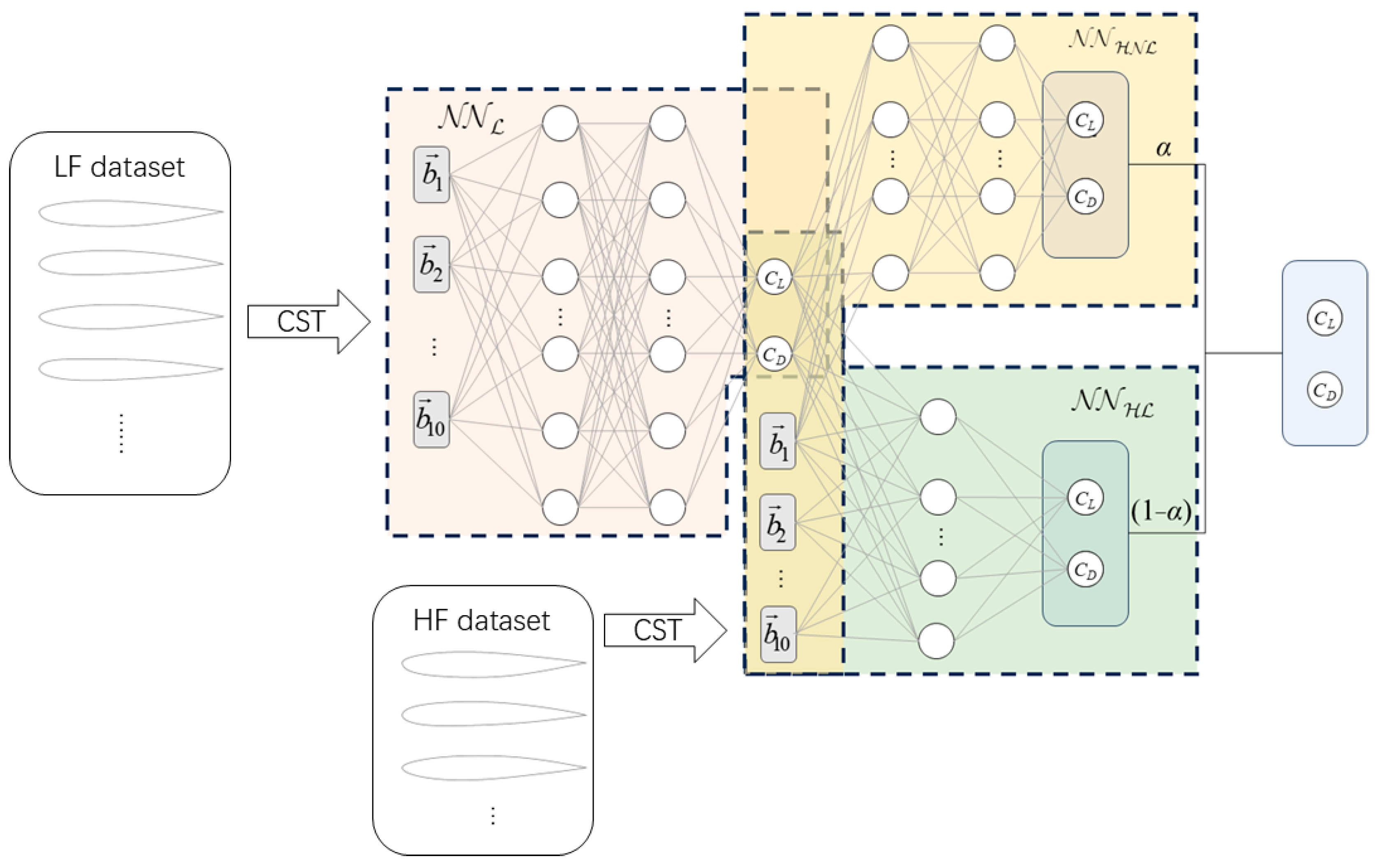
2.2. Training of Multi-Fidelity Deep Neural Networks

The multi-fidelity model is established to discover and exploit the relationships between low- and high-fidelity data, which can be expressed as

$$y_{HF}=F(y_{LF})+\delta (x)$$

(7)

where $F(•)$ is the function that maps the low-fidelity data to the high-fidelity data and $\delta (x)$ is the corresponding noise. The above equation is also written as

$$y_{HF}=\mathcal{F}(x,y_{LF})$$

(8)

To explore the linear/nonlinear correlation adaptively, $\mathcal{F}(•)$ can be divided into a linear part ${\mathcal{F}}_l$ and a nonlinear part ${\mathcal{F}}_{nl}$, i.e.,

$$y_{HF}={\mathcal{F}}_l(x,y_{LF})+{\mathcal{F}}_{nl}(x,y_{LF})$$

(9)

The multi-fidelity deep neural network model consists of three feed-forward neural networks. The first neural network, $\mathcal{N}{\mathcal{N}}_{\mathcal{L}}$, is trained using the low-fidelity data obtained from XFOIL. The second neural network, $\mathcal{N}{\mathcal{N}}_{\mathcal{H}\mathcal{L}}$, and the third neural network, $\mathcal{N}{\mathcal{N}}_{\mathcal{H}\mathcal{N}\mathcal{L}}$, trained using the high-fidelity RANS results, are employed to approximate the linear and nonlinear correlations, respectively. An additional parameter, α, is introduced to measure the linearity/nonlinearity of the correlations. The architecture of the MFDNN is presented in Figure 4. Note that b₁ to b₅ represent the 5 DVs to parameterize the upper surface of the airfoil and b₆ to b₁₀ represent the 5 DVs for the lower surface when using the CST method.

To train the MFDNN model, a loss function needs to be minimized, which consists of an LF loss function and an HF loss function

$$J({\theta }_i,{\beta }_i,{\theta }_k,{\beta }_k,\alpha )=J_{LF}({\theta }_i,{\beta }_i)+J_{HF}({\theta }_k,{\beta }_k,\alpha )$$

(10)

where

$$J_{LF}({\theta }_i,{\beta }_i)=MS{E}_{y_{LF}}+{\lambda }_{LF}{\displaystyle \sum _1^{N_{y_{LF}}}{\beta }_i^2}$$

(11)

$$\begin{array}{l}{J}_{HF}({\theta }_k,{\beta }_k,\alpha )=J_{HF}({\theta }_{k-l},{\theta }_{k-nl},{\beta }_{k-l},{\beta }_{k-nl},\alpha )\\ =MS{E}_{y_{HF}}+{\lambda }_{HF}{\displaystyle \sum _1^{N_{y_{HF}}}{{\beta }_{k-l}}^2}+{\lambda }_{HF}{\displaystyle \sum _1^{N_{y_{HF}}}{{\beta }_{k-nl}}^2}\end{array}$$

(12)

with

$$MS{E}_{y_{LF}}={\displaystyle \frac{1}{N_{y_{LF}}}}{\displaystyle \sum _1^{N_{y_{LF}}}\left[{\left|\mathcal{N}{\mathcal{N}}_{\mathcal{L}}(x_{LF},{\theta }_i,{\beta }_i)-y_{LF}\right|}^2\right]}$$

(13)

$$MS{E}_{y_{HF}}={\displaystyle \frac{1}{N_{y_{HF}}}}{\displaystyle \sum _1^{N_{y_{HF}}}\left[{\left|\begin{array}{l}\alpha \cdot \mathcal{N}{\mathcal{N}}_{\mathcal{H}\mathcal{L}}(x_{HF},{\theta }_{k-l},{\beta }_{k-l})+\\ (1-\alpha )\cdot \mathcal{N}{\mathcal{N}}_{\mathcal{H}\mathcal{N}\mathcal{L}}(x_{HF},{\theta }_{k-nl},{\beta }_{k-nl})-y_{HF}\end{array}\right|}^2\right]}$$

(14)

where $MS{E}_{y_{LF}}$ represents the mean square error (MSE) between the prediction values from $\mathcal{N}{\mathcal{N}}_{\mathcal{L}}$ and the exact values in the LF training dataset $y_{LF}$; ${\theta }_i$, ${\beta }_i$, respectively, represent the weights and biases of $\mathcal{N}{\mathcal{N}}_{\mathcal{L}}$; ${\lambda }_{LF}$ denotes the L₂ regularization parameters of $\mathcal{N}{\mathcal{N}}_{\mathcal{L}}$. Similarly, $MS{E}_{y_{HF}}$ represents the MSE between the prediction values from the weighted combination of $\mathcal{N}{\mathcal{N}}_{\mathcal{H}\mathcal{L}}$ and $\mathcal{N}{\mathcal{N}}_{\mathcal{H}\mathcal{N}\mathcal{L}}$ and the exact values $y_{HF}$ in the HF training dataset; ${\theta }_{k-l}$, ${\beta }_{k-l}$ represent the weights and biases of; ${\theta }_{k-nl}$ and ${\beta }_{k-nl}$ represent those of $\mathcal{N}{\mathcal{N}}_{\mathcal{H}\mathcal{N}\mathcal{L}}$; ${\lambda }_{HF}$ denotes the L₂ regularization parameters of $\mathcal{N}{\mathcal{N}}_{\mathcal{H}\mathcal{L}}$ and $\mathcal{N}{\mathcal{N}}_{\mathcal{H}\mathcal{N}\mathcal{L}}$, which is set to be equaled to save the computational cost.

For training the MFDNN model, a two-step training strategy is employed. Firstly, the loss function of the low-fidelity part $J_{LF}$ is minimized, and then the combined loss function of high-fidelity and low-fidelity parts, $J({\theta }_i,{\theta }_k)$, is minimized. The Adam optimizer is employed to conduct these minimizations. It should be noted that, before the training of the model, all the features and the labels are processed by Z-score normalization [52].

The performance of the MFDNN is closely related to various hyperparameters, including the numbers of layers, the number of neutrons per layer, the activation function, learning rates, epochs, and regularization rates. Some of these hyperparameters are fixed. For example, the ReLU activation function is used for the nonlinear layers; no activation function is used for linear approximations; the maximum number of epochs is set to 5000, with early stopping if no improvement is observed within 1000 epochs.

Other hyperparameters, such as the numbers of layers and neurons, learning rates, and regularization rates, are determined through the grid search method based on different training datasets. The effectiveness of these hyperparameters is assessed using a 5-fold cross-validation method, where the dataset is split into five parts—four for training and one for validation. The objective is to minimize the validation score, indicating optimal hyperparameter choices. The results of these tests and their analysis will be presented in the following section.

For practical implementation of the above process, we use the PyTorch framework (version 1.13.1). Due to inherent randomness in the training, to ensure reproducibility, we set the random seed by the command ‘torch.manual_seed(seed = 2021)’.

2.3. The Global Optimization Algorithm

This paper employs the Particle Swarm Optimization (PSO) method [53] to perform the optimizations. The PSO is a kind of global optimization algorithm that was originally intended to simulate the social behavior of birds within a flock or fish within a school. It solves an optimization problem by iteratively trying to improve a candidate solution with regard to a certain measure of quality. PSO is initialized with a group of random solutions, named particles, and then searches for optimal positions by updating generations. Each particle represents a candidate solution to the problem at hand. The particles fly through the design space by following the current optimal particles. This process is motivated by the social behavior of organisms, where each individual’s behavior is influenced by its own experience as well as the experience of neighboring individuals.

In the PSO, each particle keeps track of its coordinates in the design space which are associated with the best solution it has achieved so far, and the value is called personal best (pbest). Another best value under track is the global best value (gbest), which is the best value obtained by any particle in the population so far. At each iteration, the PSO changes the velocity of each particle toward the pbest and gbest locations. The position x_i and velocity v_i of the ith particle are updated as

$$x_i^{(t+1)}=x_i^{(t)}+\lambda \cdot v_i^{(t+1)}$$

(15)

$$v_i^{(t+1)}=w\cdot v_i^{(t)}+c_1\cdot r_1\cdot \left(pbes{t}_i-x_i^{(t)}\right)+c_2\cdot r_2\cdot \left(gbest-x_i^{(t)}\right)$$

(16)

where t represents the current iteration, $\lambda$ is the relax factor of velocity that prevents the excessive speed of the particle movement, $w$ is the inertia weight which controls the impact of the previous velocities on the current velocity, $c_1$ and $c_2$ are cognitive and social parameters, respectively, $r_1$ and $r_2$ are the learning factors with random numbers in the range [0, 1] which introduce stochastic elements to the system, $pbes{t}_i$ is the best known position of particle i, and $gbest$ is the best known position among all the particles. Note that the upper and lower bounds of the position are set as 50% and −50% of the initial values of b_i, and those of the velocity are set as 20% and −20% of the differences between the upper and lower bounds of b_i. To perform a PSO, the following steps are employed.

(1)

Initialize a population of particles with random positions and velocities within defined bounds.

(2)

Evaluate the objective function F_obj for each particle.

(3)

Update the personal best position of each particle.

(4)

Update the global best position of all particles.

(5)

Evaluate and update the velocity and position of the particles according to Equations (15) and (16).

(6)

Repeat steps 2–5 until the stopping criterion is met.

Here, the initialization of the particles uses the LHS method to generate a population of 30 particles, ensuring consistent conditions in all cases. Since the ASO problem considered in this paper involves constraints, the objective function is constructed using the exterior penalty function method. The used parameters in Equations (15) and (16) will be presented in Section 4. As random numbers $r_1$ and $r_2$ exist in the PSO, the command ‘numpy.random.seed(52)’ is used to ensure reproducibility.

To make it more clearly, the framework of the whole process for aerodynamic prediction and design optimization based on the MFDNN is presented in Figure 5.

3. Aerodynamic Coefficient Predictions Using MFDNN Models

3.1. Description of the Aerodynamic Prediction Task

Before applying the MFDNN models to the ASO problems, we first investigate the effects of the HF/LF data ratio on the prediction accuracy. Several values of HF/LF data ratios are considered, i.e., 20/200, 40/200, 60/200, 80/200, 100/200, 120/200. The performance of the MFDNN model is compared with the traditional SFNN model and for a fair comparison, the same numbers of HF data are considered in the traditional SFNN model, i.e., 20, 40, 60, 80, 100, 120.

The fifth-order CST parameterization method is employed to each surface of the airfoil to parameterize its shape. The upper and lower limits of the design variables are set as 150% and 50% of the baseline values b_i obtained by fitting the NACA 0012 airfoil. These values are detailed in

Table 1. The baseline values and upper and lower limits of b_i used in the CST parameterization method.

	Upper Surface			Lower Surface
	Baseline	Upper Bound	Lower Bound	Baseline	Upper Bound	Lower Bound
b0	0.160612	0.240918	0.080306	−0.160612	−0.080306	−0.240918
b1	0.1200491	0.1800737	0.0600246	−0.120049	−0.060025	−0.180074
b2	0.1792529	0.2688794	0.0896265	−0.179253	−0.089627	−0.268879
b3	0.1776805	0.2665208	0.0888403	−0.177681	−0.088840	−0.266521
b4	0.1881634	0.2822451	0.0940817	−0.188163	−0.094082	−0.282245

.

To generate the sample airfoils used for establishing the training dataset, all the values b_i are obtained by the Sobol sequence method as described in Section 2. Note that, when the number of the HF data increase, the samples that had been used in the lower number cases are still kept. For testing the prediction accuracy of the established models, another 20 test airfoils are generated by the LHS method. The sample airfoils in the training dataset and test dataset are presented in Figure 6 and Figure 7, respectively.

To obtain the labels of the data, the C_L and C_D of the sample airfoils are evaluated under specific flow conditions consisting of the Reynolds (Re) number 438000, the freestream Mach (Ma) number 0.3 and the angle of attack (AOA) 5°. Recall that the low-fidelity data are obtained from XFOIL and the high-fidelity data are obtained by numerically solving the RANS equations.

Based on the training dataset, the MFDNN and SFNN models are trained by the methods presented in Section 2.2. It has been demonstrated above that the hyperparameters of the MFDNN model have decisive impact on the performance of the models, and the main purpose of training the model is to obtain the optimal hyperparameters. The hyperparameters that need to be searched include the learning rate (LR), the number of hidden layers, the number of neurons in each layer, and the regularization rates.

3.2. Training Results of the Models

A grid search method is employed to find optimal hyperparameters, and this progress is conducted by three stages The first one is to find hyperparameters for $\mathcal{N}{\mathcal{N}}_{\mathcal{L}}$. The learning rates of 0.1, 0.001, 0.0001, 0.00001, the numbers of hidden layers ranging from 1 to 7, and the numbers of neurons per layer ranging from 20 to 70 are tested. The optimal hyperparameters are identified as LR of 0.01, and 2 hidden layers with each layer containing 60 neurons. The second stage is to find hyperparameters for $\mathcal{N}{\mathcal{N}}_{\mathcal{H}\mathcal{L}}$ and $\mathcal{N}{\mathcal{N}}_{\mathcal{H}\mathcal{N}\mathcal{L}}$. Note that, the number of neurons for $\mathcal{N}{\mathcal{N}}_{\mathcal{H}\mathcal{L}}$ is set equal to that for $\mathcal{N}{\mathcal{N}}_{\mathcal{H}\mathcal{N}\mathcal{L}}$ to reduce the computational costs. The optimal hyperparameters identified include a learning rate (LR) of 0.01 and a network architecture consisting of 5 hidden layers, each containing 5 neurons. The third stage is to find optimal regularization rates (denoted as ${\lambda }_{LF}$ and ${\lambda }_{HF}$). As the LF data are fixed, the optimal value of ${\lambda }_{LF}$ is identified as 0.001. Whereas, the HF data vary, so the values of ${\lambda }_{HF}$ ranging from 0.01 to 0.0000001 are tested for each model. The mean square errors (MSE) between the predictions and the labels of the test dataset are shown in

Table 2. Mean square errors when using various regulation rates ${\lambda }_{HF}$ for training the MFDNN and SFNN models. (a) MSE of the MFDNN models tested on the test dataset. (b) MSE of the SFNN models tested on the test dataset.

(a)
Data (LF/HF)	λHF
	0.01	0.001	0.0001	0.00001	0.000001	0.0000001
200/20	3.35 × 10−5	2.47 × 10−5	1.24 × 10−5	1.60 × 10−5	1.47 × 10−5	1.27 × 10−5
200/40	1.18 × 10−5	1.13 × 10−5	3.87 × 10−6	7.09 × 10−6	9.30 × 10−6	8.00 × 10−6
200/60	1.03 × 10−5	1.03 × 10−5	1.06 × 10−5	3.94 × 10−6	2.72 × 10−6	6.14 × 10−6
200/80	1.05 × 10−5	9.99 × 10−6	8.87 × 10−6	2.17 × 10−6	1.99 × 10−6	8.96 × 10−6
200/100	1.05 × 10−5	9.56 × 10−6	9.39 × 10−6	1.45 × 10−6	1.54 × 10−6	4.36 × 10−6
200/120	1.08 × 10−5	9.83 × 10−6	1.00 × 10−5	1.32 × 10−6	2.11 × 10−6	2.37 × 10-−6
(b)
Data (HF)	λHF
	0.01	0.001	0.0001	0.00001	0.000001	0.0000001
20	7.64 × 10−5	6.99 × 10−5	6.92 × 10−5	3.27 × 10−4	3.39 × 10−4	3.35 × 10−4
40	6.71 × 10−5	6.96 × 10−5	5.93 × 10−5	1.90 × 10−4	1.67 × 10−4	1.43 × 10−4
60	1.87 × 10−5	1.36 × 10−5	1.17 × 10−5	4.04 × 10−5	6.55 × 10−5	6.24 × 10−5
80	1.05 × 10−5	7.96 × 10−6	1.22 × 10−5	3.42 × 10−5	4.19 × 10−5	4.89 × 10−5
100	1.35 × 10−5	5.99 × 10−6	6.32 × 10−6	2.80 × 10−5	2.60 × 10−5	2.33 × 10−5
120	1.23 × 10−5	6.53 × 10−6	5.14 × 10−6	2.74 × 10−5	3.20 × 10−5	1.62 × 10−5

with the best MSE highlighted with underlines.

The results presented in Table 2 show that the optimal regularization rates ${\lambda }_{HF}$ vary depending on the quantities of HF data. For training the MFDNN models, employing ${\lambda }_{HF}$ of 0.0001 achieves the lowest MSE when using 20/40 HF data, while 0.000001 for using 60/80 HF data, and 0.00001 for using 100/120 HF data. For training the SFNN models, employing ${\lambda }_{HF}$ of 0.0001 achieves the lowest MSE when using 20/40/60/120 HF data, while 0.001 for using 80/100 HF data. From these results, it can be found that the value of the regularization rate has significant impact on the performance of the models, and an appropriate choice can notably reduce the MSE.

The effects of using ReLU and Tanh as the activation functions are tested, and the results are shown in

Table 3. Mean square errors when using various activate functions of ReLU and Tanh.

MFDNN			SFNN
Data (LF/HF)	Tanh	ReLU	Data (HF)	Tanh	ReLU
200/20	3.31 × 10−5	1.24 × 10−5	20	1.11 × 10−4	6.92 × 10−5
200/40	1.22 × 10−5	3.87 × 10−6	40	6.46 × 10−5	5.93 × 10−5
200/60	7.40 × 10−6	2.72 × 10−6	60	2.55 × 10−5	1.17 × 10−5
200/80	9.55 × 10−6	1.99 × 10−6	80	1.88 × 10−5	7.96 × 10−6
200/100	4.82 × 10−5	1.45 × 10−6	100	7.59 × 10−6	5.99 × 10−6
200/120	1.41 × 10−6	1.32 × 10−6	120	6.55 × 10−6	5.14 × 10−6

.

The results in Table 3 show that for both MFDNN and SFNN models, using the ReLU as the activate function can achieve lower MSE than the Tanh. Thus, the ReLU will be employed in the following tests.

After completing the three stages, the optimal hyperparameters for each model are summarized in

Table 4. Optimal hyperparameters for training the MFDNN and SFNN models. (a) Optimal hyperparameters for the MFDNN models. (b) Optimal hyperparameters for the SFNN models.

(a)
HF Data	LR	λLF	λHF	$\mathcal{N}{\mathcal{N}}_{\mathcal{L}}$		$\mathcal{N}{\mathcal{N}}_{\mathcal{H}\mathcal{L}}$	$\mathcal{N}{\mathcal{N}}_{\mathcal{H}\mathcal{N}\mathcal{L}}$
				Layers	Neurons	Neurons	Layers	Neurons
20/40	0.01	0.001	1 × 10−4	2	60	50	5	40
60/80	0.01	0.001	1 × 10−6	2	60	50	5	40
100/120	0.01	0.001	1 × 10−5	2	60	50	5	40
(b)
HF Data				LR		λHF	Layers	Neurons
20/40/60/120				0.01		1 × 10−4	5	40
80/100				0.01		1 × 10−3	5	40

.

3.3. Examination of Accuracy and Efficiency

After training each model with the corresponding optimal hyperparameters, the prediction accuracy on the 20 test airfoils is examined. Note that, the C_L and C_D values directly obtained by RANS are assumed to be accurate solutions. The L₂ norm errors and the maximum errors between the predicted values of each model and the accurate values are presented in Figure 8, and the time costs to construct the training dataset of each situation are shown in

Table 5. Time costs of constructing the training database of MFDNN and SFNN models using various quantities of data.

Data (LF/HF)	MFDNN Time (Minutes)	Data (HF)	SFNN Time (Minutes)
200/20	80.80	20	64.50
200/40	147.60	40	131.30
200/60	214.32	60	198.02
200/80	281.05	80	264.75
200/100	347.85	100	331.55
200/120	414.58	120	398.28

.

As shown in Figure 8, when the same quantity of HF data are employed, almost all the MFDNN models achieve significantly lower L2 errors and maximum errors than the SFNN models. These results indicate that introducing LF data and developing the MFDNN models is effective in improving the prediction accuracy of the aerodynamic coefficients. Specifically, the less HF data used, the larger the error gap between the MFDNN and SFNN models.

From the time costs shown in Table 5, it can be observed that the MFDNN model trained with 200 LF and 40 HF data requires less time to obtain training data than the SFNN models trained with 60, 80, and 100 HF data. However, as the results shown in Figure 8, the former model can achieve higher prediction accuracy than the latter. This indicates that when the same time cost is required to obtain training data, the MFDNN provides better prediction accuracy than the SFNN. Since obtaining HF data using CFD is expensive, the efficiency of MFDNN in constructing the training dataset is particularly desirable.

4. Aerodynamic Shape Optimization Using MFDNN Models

A global optimization typically requires thousands of objective function evaluations, which makes the time cost of employing CFD unacceptable. To solve this problem, a surrogate model is usually employed. Since the presented MFDNN models can be employed as surrogate models, this section focuses on applying them in a practical ASO problem.

4.1. Description of the Aerodynamic Shape Optimization Problem

A specific aerodynamic shape optimization problem with a single objective function subject to an equality constraint in the flow condition is considered. The flow conditions are the same as in the last section, i.e., Re = 438000, Ma = 0.3, and AOA = 5°. This ASO problem can be summarized as

minimize C_D

s.t. C_L = 0.52

To perform the ASO, the PSO optimization algorithm is employed, and the parameters used in the PSO are presented in

Table 6. Parameters used in the PSO optimization algorithm.

Parameters	Values
Number of particles	30
Inertia	0.5
Global increment	2
Particle increment	2
Velocity limitation	10%
Max iterations	200

. The bounds of the DVs are set as 150% and 50% of the baseline values (see Table 1). The exterior penalty function method is employed, which modifies the objective function as

$$F_{\mathrm{obj}}={\omega }_{eq}\cdot {[S_{CL}\cdot (C_L-0.52)]}^2+S_{CD}\cdot C_D$$

(17)

where ${\omega }_{eq}$ is the weight of the constraint function in the objective function and is set as 1000. The $S_{CL}$ and $S_{CD}$ are the scale factors of the aerodynamic coefficients, which are set to 100 and 10,000, respectively. This ensures that both coefficients are of the same order of magnitude and are consistent with the previously defined “counts”.

4.2. Optimization Results Using the Non-Updated MFDNN Models

The MFDNN models trained using 200 LF data combined with various quantities of HF data (20, 40, 60, 80, 100, and 120) and the SFNN models trained using the same HF datasets are utilized to perform the optimization. It is noted that the $C_L$ of the initial NACA 0012 is 0.52, and the $C_D$ is 0.014457. For $C_L$, one count equals 0.01, while for $C_D$, one count equals 0.0001. The optimal shapes are presented in Figure 9.

It can be seen from Figure 9 that there are differences between the optimal shapes obtained by employing different quantities of HF/LF data for training the models. The detailed results of the optimizations are shown in

Table 7. Comparison of the optimization results using the MFDNN and the SFNN models trained with various quantities of HF/LF data.

	MFDNN			SFNN
	CL (Counts)	CD (Counts)	Fobj	CL (Counts)	CD (Counts)	Fobj
200–20	52.0	134.65	134.65	52.0	139.56	139.56
200–40	52.0	130.25	130.25	52.0	138.18	138.18
200–60	52.0	131.81	131.81	52.0	138.36	138.36
200–80	52.0	131.23	131.23	52.0	137.43	137.43
200–100	52.0	131.18	131.18	52.0	136.87	136.87
200–120	52.0	132.71	132.71	52.0	136.23	136.23

.

It can be seen from Table 7 that optimizations using both the MFDNN and SFNN models reduce $C_D$ successfully. Specifically, the MFDNN models consistently achieve lower $C_D$ compared to the SFNN models, and using the extra 200 LF data for training the MFDNN models leads to a reduction in $C_D$ by approximately 5 more counts. Moreover, the optimal $C_D$ obtained by employing 20 HF data for the MFDNN model is lower than that obtained by employing 120 HF data for the SFNN model. This demonstrates that, with the need of fewer HF data, the MFDNN can achieve a better optimization result.

In the process of obtaining the training dataset, calculating one HF datum takes approximately 3 min, whereas calculating one LF datum only takes about 1.5 s. Thus, the time cost of obtaining 20 HF data for the MFDNN model is significantly lower than that of obtaining 120 HF for the SFNN model, which can demonstrate the advantage in efficiency when using the MFDNN models in an ASO.

As shown in Table 7, increasing the HF data typically improves the optimization results when using the SFNN model; however, this trend is not appropriate for the MFDNN model, and the MFDNN model trained with 40 HF data obtained the best result. This phenomenon indicates that a higher HF/LF data ratio does not definitely result in a better performance in an ASO when using MFDNN models. For the ASO problem presented in this paper, the optimal HF/LF data ratio is 20%.

The optimization histories using different models are presented in Figure 10.

As shown in Figure 10, the value of F_obj obtained from the SFNN models tends to plateau after 50 iterations, while that from the MFDNN model continues to decrease until 200 iterations. This indicates that the design space explored by the MFDNN models is more extensive than that of the SFNN models.

Furthermore, we examine the errors between the aerodynamic coefficients of the optimal shapes obtained by the MFDNN/SFNN models and by the CFD, which are presented in

Table 8. Comparison of the errors of the optimization results obtained by employing the MFDNN and the SFNN models. (a) MFDNN models. (b) SFNN models.

(a)
	CL (Counts)			CD (Counts)			Fobj
LF-HF Data	MFDNN	CFD	Error	MFDNN	CFD	Error	MFDNN	CFD
200–20	52.00	50.26	1.74	134.65	133.55	1.09	134.65	3159.76
200–40	52.00	50.03	1.97	130.25	133.24	2.99	130.25	4010.26
200–60	52.00	50.17	1.83	131.81	133.89	2.08	131.81	3475.96
200–80	52.00	50.36	1.64	131.23	132.79	1.56	131.23	2811.38
200–100	52.00	50.35	1.65	131.18	131.76	0.58	131.18	2868.12
200–120	52.00	50.91	1.09	132.71	133.54	0.83	132.71	1331.05
(b)
	CL (Counts)			CD (Counts)			Fobj
HF Data	SFNN	CFD	Error	SFNN	CFD	Error	SFNN	CFD
20	52.00	51.16	0.84	139.56	137.34	2.21	139.56	846.17
40	52.00	51.29	0.71	138.18	135.00	3.19	138.18	642.12
60	52.00	51.66	0.34	138.36	135.70	2.66	138.36	249.02
80	52.00	51.64	0.36	137.43	136.05	1.38	137.43	267.28
100	52.00	52.77	0.77	136.87	133.30	3.57	136.87	720.42
120	52.00	51.93	0.07	136.23	133.92	2.31	136.23	138.99

.

The results from Table 8 show that errors exist between the prediction values and the accurate values of $C_L$ and $C_D$. Although the $C_D$ has been reduced successfully, it is preferred to eliminate these errors. Thus, we will introduce an approach of updating the MFDNN models during the optimization to solve this problem.

4.3. Optimization Results Using the Updated MFDNN Models

The updated MFDNN model is established based on the distance between the global best position obtained in the current iteration and the global best position where the model is updated for the last time. Assuming that the current global best position is ${\overrightarrow{x}}_{g\_best,i}$, and the global best position when we update the model for the last time is ${\overrightarrow{x}}_{g\_best,last}$, the Euclidean distance between these two positions is calculated by

$${\mathrm{\Phi }}_i={‖{\overrightarrow{x}}_{g\_best,i}-{\overrightarrow{x}}_{g\_best,last}‖}_2$$

(18)

By setting a predefined threshold $\mathrm{{\rm T}}$, when ${\mathrm{\Phi }}_i<\mathrm{{\rm T}}$, the model keeps fixed, and when ${\mathrm{\Phi }}_i\ge \mathrm{{\rm T}}$, the model is updated by conducting the transfer learning. The new training dataset is constructed by evaluating one extra HF datum and one extra LF datum at the position of ${\overrightarrow{x}}_{g\_best,i}$. In this study, we set $\mathrm{{\rm T}}$ equals 0.03, and the new optimal shapes are presented in Figure 11.

As shown in Figure 11, the similarity of the optimal shapes obtained by using the updated models with various quantities of HF data is higher than that by using non-updated models. The detailed results of the optimizations are shown in

Table 9. Comparison of the errors of the optimization results obtained by employing the updated MFDNN and the SFNN models. (a) Updated MFDNN models. (b) Updated SFNN models.

(a)
	CL (Counts)			CD (Counts)			Fobj
LF-HF Data	MFDNN	CFD	Error	MFDNN	CFD	Error	MFDNN	CFD
200–20	52.00	51.95	0.05	133.60	133.59	0.01	133.61	135.91
200–40	51.99	51.99	0.00	132.58	132.66	0.07	132.78	132.83
200–60	52.00	51.89	0.11	133.01	132.94	0.07	133.01	144.77
200–80	52.01	52.05	0.04	134.60	134.67	0.07	134.66	137.25
200–100	51.98	51.92	0.06	133.91	134.05	0.14	134.21	139.92
200–120	52.00	51.95	0.05	131.80	132.56	0.77	131.80	135.22
(b)
	CL (Counts)			CD (Counts)			Fobj
HF Data	SFNN	CFD	Error	SFNN	CFD	Error	SFNN	CFD
20	52.00	52.27	0.27	137.97	136.40	1.57	137.97	210.99
40	52.00	52.08	0.08	137.34	135.96	1.38	137.34	141.62
60	52.00	51.98	0.02	139.22	137.40	1.82	139.22	137.97
80	52.00	51.90	0.10	137.46	136.86	0.60	137.46	147.45
100	52.00	52.17	0.17	137.82	137.60	0.22	137.84	167.35
120	51.98	52.01	0.03	136.39	136.39	0.00	136.92	136.42

.

The results presented in Table 9 show significant decrease in prediction errors for the updated MFDNN models. The errors are generally below 0.15 counts, except the 200-120 case for $C_D$. It demonstrates that the update strategy has effectively addressed the previous inadequacies in the MFDNN models, i.e., the prediction errors of the optimal shapes. Comparing the performances between the MFDNN and the SFNN models, the update strategy significantly benefits the MFDNN models, while, for the updated SFNN models, it does not exhibit any improvement in $C_D$ compared to the non-updated models.

The update strategy can improve the accuracy, but it also introduces extra time costs due to the need of evaluating some new data during the ASO. Although the cost is acceptable, we still consider further enhancing the efficiency of the presented update strategy by introducing a dual-threshold (DT) update strategy for the MFDNN models. Specifically, we divide the threshold $\mathrm{{\rm T}}$ into two levels, i.e., ${\mathrm{{\rm T}}}_{\mathrm{HF}}$ and ${\mathrm{{\rm T}}}_{\mathrm{LF}}$. When ${\mathrm{\Phi }}_{ji}\ge {\mathrm{{\rm T}}}_{\mathrm{LF}}$, LF data are evaluated and added to the training dataset, but the model is kept fixed; when ${\mathrm{\Phi }}_{ji}\ge {\mathrm{{\rm T}}}_{\mathrm{HF}}$, HF data are evaluated and the model is updated. By this way, some HF evaluations are substituted with LF ones to reduce time costs. In this study, we set ${\mathrm{{\rm T}}}_{\mathrm{LF}}$ equals 0.03 and ${\mathrm{{\rm T}}}_{\mathrm{HF}}$ equals 0.05. The results for employing this dual-threshold multi-fidelity deep neural network (DTMFDNN) models are shown in

Table 10. Comparison of the errors of the optimization results obtained by employing the dual-threshold updated MFDNN models.

	CL (Counts)			CD (Counts)			Fobj
HF Data	DTMFDNN	CFD	Error	DTMFDNN	CFD	Error	DTMFDNN	CFD
20	51.99	51.97	0.03	132.74	133.65	0.92	132.80	134.77
40	52.01	51.97	0.04	133.67	133.58	0.09	133.74	134.76
60	52.00	51.96	0.04	132.83	132.97	0.14	132.85	134.50
80	52.00	52.04	0.04	131.72	133.80	2.08	131.72	135.64
100	52.00	51.96	0.04	131.97	133.65	1.68	131.97	135.64
120	51.99	51.92	0.07	135.41	135.86	0.45	135.46	142.17

.

As shown in Table 10, the optimization results obtained using the dual-threshold update strategy are comparable to those using the normal update strategy. The CFD and XFOIL calls are show in

Table 11. Comparison of CFD and XFOIL calls using the single-threshold and dual-threshold update strategy for the MFDNN models.

	Single-Threshold Update Strategy		Dual-Threshold Update Strategy
LF-HF Data	CFD	XFOIL	CFD	XFOIL
200–20	23	23	13	88
200–40	29	29	16	67
200–60	25	25	15	85
200–80	23	23	12	79
200–100	13	13	9	87
200–120	22	22	8	100

.

As shown in Table 11, the results show that the CFD calls when employing the DTMFDNN models are nearly half of those when using the single threshold. Although the counts for XFOIL evaluations increase by one to two times. It is acceptable because the evaluation of an LF datum takes only about 1.5 s. These results confirm that employing the DTMFDNN models can significantly reduce the time costs, without worsening the optimization results. So far, a framework of an ASO based on the DTMFDNN model is developed, which can balance the efficiency and the optimization quality.

5. Conclusions

This paper investigates the performance of the MFDNN models in predictions of aerodynamic coefficients and performing the aerodynamic shape optimizations, especially, the impact of the HF/LF data ratio. The results of prediction accuracy show that when the same HF data are employed, less HF data are used, and more advantage in accuracy can be achieved by the MFDNN models than the SFNN. This is because its prediction accuracy is less sensitive to the quantity of HF data compared to the SFNN model when the LF data are introduced in the training. Additionally, the MFDNN model trained by 200 LF and 40 HF data achieved higher accuracy than the SFNN models trained by 60, 80, and 100 HF data. Whereas, the former one uses much less time when constructing the training dataset. It indicates that when the same time cost is required to obtain training data, the MFDNN can achieve better prediction accuracy. For performing the ASO, non-updated models are employed first. The results show that employing higher HF/LF data ratios for training MFDNN models may not result in better optimization results. For the presented study in this paper, using a ratio of 20% obtains the best result. This finding provides a reference for other researchers who want to employ the MFDNN models that employing more HF data may not be absolutely better. To solve the insufficiency of the prediction accuracy for the optimal shapes, a distance-based update strategy is introduced, and the results using updated MFDNN models show high accuracy. To further reduce the time cost, we developed a dual-threshold update strategy for the MFDNN models which is named DTMFDNN. By using these strategies, an efficient ASO framework that tightly integrates PSO with updated MFDNN models is construed. However, there are two limitations to the present study. First, the used grid search method to optimize the hyperparameters is time-consuming; a more efficient method such as Bayesian optimization is preferred. The second limitation is that when using a relatively large number of HF data in the MFDNN models, the optimization results tend to become worse. The mechanism of this phenomenon is not well understood, and deeper investigations are being conducted.

References

1. Box, G.E.P.; Wilson, K.B. On the Experimental Attainment of Optimum Conditions. J. R. Stat. Soc. Ser. B Methodol. 1951, 13, 270–310. [Google Scholar] [CrossRef]
2. Haftka, R.T.; Scott, E.P.; Cruz, J.R. Optimization and Experiments: A Survey. Appl. Mech. Rev. 1998, 51, 435–448. [Google Scholar] [CrossRef]
3. Simpson, T.W.; Poplinski, J.D.; Koch, P.N.; Allen, J.K. Metamodels for computer-based engineering design: Survey and recommendations. J. Eng. Comput. 2001, 17, 129–150. [Google Scholar] [CrossRef]
4. Myers, R.H.; Montgomery, D.C.; Anderson-Cook, C.M. Response Surface Methodology: Process and Product Optimization Using Designed Experiments; John Wiley & Sons: New York, NY, USA, 2016. [Google Scholar]
5. Engelund, W.C.; Stanley, D.O.; Lepsch, R.A.; McMillin, M.M.; Unal, R. Aerodynamic configuration design using response surface methodology analysis. In Proceedings of the Aircraft Design, Systems, and Operations Meeting, Monterey, CA, USA, 1 August 1993; p. 10718. [Google Scholar]
6. Vavalle, A.; Qin, N. Iterative Response Surface Based Optimization Scheme for Transonic Airfoil Design. J. Aircr. 2007, 44, 365–376. [Google Scholar] [CrossRef]
7. Krige, D.G. A statistical approach to some basic mine valuation problems on the Witwatersrand. J. S. Afr. Inst. Min. Metall. 1951, 52, 119–139. [Google Scholar]
8. Matheron, G. Principles of geostatistics. Econ. Geol. 1963, 58, 1246–1266. [Google Scholar] [CrossRef]
9. Simpson, T.W.; Mauery, T.M.; Korte, J.J.; Mistree, F. Kriging Models for Global Approximation in Simulation-Based Multidisciplinary Design Optimization. AIAA J. 2001, 39, 2233–2241. [Google Scholar] [CrossRef]
10. Jeong, S.; Murayama, M.; Yamamoto, K. Efficient Optimization Design Method Using Kriging Model. J. Aircr. 2005, 42, 413–420. [Google Scholar] [CrossRef]
11. Liu, W.; Batill, S. Gradient-Enhanced Response Surface Approximations Using Kriging Models. In Proceedings of the 9th AIAA/ISSMO Symposium on Multidisciplinary Analysis and Optimization, Atlanta, GA, USA, 4–6 September 2002. [Google Scholar]
12. Laurenceau, J.; Sagaut, P. Building Efficient Response Surfaces of Aerodynamic Functions with Kriging and Cokriging. AIAA J. 2008, 46, 498–507. [Google Scholar] [CrossRef]
13. Chung, H.S.; Alonso, J. Using gradients to construct cokriging approximation models for high-dimensional design optimization problems. In Proceedings of the 40th AIAA Aerospace Sciences Meeting & Exhibit, Reno, NV, USA, 14–17 January 2002. [Google Scholar]
14. Han, Z. Kriging surrogate model and its application to design optimization: A review of recent progress. Hangkong Xuebao/Acta Aeronaut. Astronaut. Sin. 2016, 37, 3197–3225. (In Chinese) [Google Scholar] [CrossRef]
15. Buhmann, M.D. Radial basis functions. Acta Numer. 2000, 9, 1–38. [Google Scholar] [CrossRef]
16. Wendland, H. Scattered Data Approximation; Cambridge University Press: Cambridge, UK, 2004; Volume 17, p. x+336. [Google Scholar]
17. Tyagi, A.; Singh, P.; Rao, A.; Kumar, G.; Singh, R.K. A novel framework for optimizing Gurney flaps using RBF surrogate model and cuckoo search algorithm. Acta Mech. 2024, 235, 3385–3404. [Google Scholar] [CrossRef]
18. Zhou, Z.; Ong, Y.S.; Nair, P.B.; Keane, A.J.; Lum, K.Y. Combining Global and Local Surrogate Models to Accelerate Evolutionary Optimization. IEEE Trans. Syst. Man Cybern. Part C Appl. Rev. 2007, 37, 66–76. [Google Scholar] [CrossRef]
19. Queipo, N.V.; Haftka, R.T.; Shyy, W.; Goel, T.; Vaidyanathan, R.; Kevin Tucker, P. Surrogate-based analysis and optimization. Prog. Aerosp. Sci. 2005, 41, 1–28. [Google Scholar] [CrossRef]
20. Yakowitz, S.J.; Szidarovszky, F. A comparison of kriging with nonparametric regression methods. J. Multivar. Anal. 1985, 16, 21–53. [Google Scholar] [CrossRef]
21. Santos, M.; Mattos, B.; Girardi, R. Aerodynamic Coefficient Prediction of Airfoils Using Neural Networks. In Proceedings of the 46th AIAA Aerospace Sciences Meeting and Exhibit, Reno, Nevada, USA, 7–10 January 2008. [Google Scholar]
22. Zhang, Y.; Sung, W.J.; Mavris, D.N. Application of Convolutional Neural Network to Predict Airfoil Lift Coefficient. In Proceedings of the 2018 AIAA/ASCE/AHS/ASC Structures, Structural Dynamics, and Materials Conference, Kissimmee, FL, USA, 8–12 January 2018. [Google Scholar]
23. Andrés-Pérez, E.; Carro-Calvo, L.; Salcedo-Sanz, S.; Martin-Burgos, M.J. Aerodynamic Shape Design by Evolutionary Optimization and Support Vector Machines; Springer International Publishing: Cham, Switzerland, 2016. [Google Scholar]
24. Bouhlel, M.A.; He, S.; Martins, J.R.R.A. Scalable gradient–enhanced artificial neural networks for airfoil shape design in the subsonic and transonic regimes. Struct. Multidiscip. Optim. 2020, 61, 1363–1376. [Google Scholar] [CrossRef]
25. Du, X.; He, P.; Martins, J.R.R.A. Rapid airfoil design optimization via neural networks-based parameterization and surrogate modeling. Aerosp. Sci. Technol. 2021, 113, 106701. [Google Scholar] [CrossRef]
26. Li, J.; Du, X.; Martins, J.R.R.A. Machine learning in aerodynamic shape optimization. Prog. Aerosp. Sci. 2022, 134, 100849. [Google Scholar] [CrossRef]
27. Forrester, A.I.J.; Sóbester, A.; Keane, A.J. Multi-fidelity optimization via surrogate modelling. Proc. R. Soc. A Math. Phys. Eng. Sci. 2007, 463, 3251–3269. [Google Scholar] [CrossRef]
28. Kennedy, M.; O’Hagan, A. Predicting the output from a complex computer code when fast approximations are available. Biometrika 2000, 87, 1–13. [Google Scholar] [CrossRef]
29. Han, Z.-H.; Görtz, S. Hierarchical Kriging Model for Variable-Fidelity Surrogate Modeling. AIAA J. 2012, 50, 1885–1896. [Google Scholar] [CrossRef]
30. Han, Z.; Xu, C.; Zhang, L.; Zhang, Y.; Zhang, K.; Song, W. Efficient aerodynamic shape optimization using variable-fidelity surrogate models and multilevel computational grids. Chin. J. Aeronaut. 2020, 33, 31–47. [Google Scholar] [CrossRef]
31. Shi, M.; Lv, L.; Sun, W.; Song, X. A multi-fidelity surrogate model based on support vector regression. Struct. Multidiscip. Optim. 2020, 61, 2363–2375. [Google Scholar] [CrossRef]
32. Tao, J.; Sun, G. Application of deep learning based multi-fidelity surrogate model to robust aerodynamic design optimization. Aerosp. Sci. Technol. 2019, 92, 722–737. [Google Scholar] [CrossRef]
33. Meng, X.; Karniadakis, G.E. A composite neural network that learns from multi-fidelity data: Application to function approximation and inverse PDE problems. J. Comput. Phys. 2020, 401, 109020. [Google Scholar] [CrossRef]
34. Zhang, X.; Xie, F.; Ji, T.; Zhu, Z.; Zheng, Y. Multi-fidelity deep neural network surrogate model for aerodynamic shape optimization. Comput. Methods Appl. Mech. Eng. 2021, 373, 113485. [Google Scholar] [CrossRef]
35. Yang, A.; Li, J.; Liem, R.P. Multi-fidelity Data-driven Aerodynamic Shape Optimization of Wings with Composite Neural Networks. In Proceedings of the AIAA AVIATION 2023 Forum, San Diego, CA, USA, 12–16 June 2023. [Google Scholar]
36. Li, Z.; Montomoli, F.; Casari, N.; Pinelli, M. High-Dimensional Uncertainty Quantification of High-Pressure Turbine Vane Based on Multi-Fidelity Deep Neural Networks. In Proceedings of the ASME Turbo Expo 2023: Turbomachinery Technical Conference and Exposition, Boston, MA, USA, 26–30 June 2023. [Google Scholar]
37. Wu, X.; Zuo, Z.; Ma, L.; Zhang, W. Multi-fidelity neural network-based aerodynamic optimization framework for propeller design in electric aircraft. Aerosp. Sci. Technol. 2024, 146, 108963. [Google Scholar] [CrossRef]
38. Nagawkar, J.R.; Leifsson, L.T.; He, P. Aerodynamic Shape Optimization Using Gradient-Enhanced Multifidelity Neural Networks. In Proceedings of the AIAA SCITECH 2022 Forum, San Diego, CA, USA, 3–7 January 2022. [Google Scholar]
39. Tao, G.; Fan, C.; Wang, W.; Guo, W.; Cui, J. Multi-fidelity deep learning for aerodynamic shape optimization using convolutional neural network. Phys. Fluids 2024, 36, 056116. [Google Scholar] [CrossRef]
40. Geng, X.; Liu, P.; Hu, T.; Qu, Q.; Dai, J.; Lyu, C.; Ge, Y.; Akkermans, R.A.D. Multi-fidelity optimization of a quiet propeller based on deep deterministic policy gradient and transfer learning. Aerosp. Sci. Technol. 2023, 137, 108288. [Google Scholar] [CrossRef]
41. Liao, P.; Song, W.; Du, P.; Zhao, H. Multi-fidelity convolutional neural network surrogate model for aerodynamic optimization based on transfer learning. Phys. Fluids 2021, 33, 127121. [Google Scholar] [CrossRef]
42. Kulfan, B.; Bussoletti, J. “Fundamental” Parameteric Geometry Representations for Aircraft Component Shapes. In Proceedings of the 11th AIAA/ISSMO Multidisciplinary Analysis and Optimization Conference, Portsmouth, VI, USA, 6–8 September 2006. [Google Scholar]
43. Kulfan, B. A Universal Parametric Geometry Representation Method—“CST”. In Proceedings of the 45th AIAA Aerospace Sciences Meeting and Exhibit, Reno, NV, USA, 8–11 January 2007. [Google Scholar]
44. van Ingen, J. The eN Method for Transition Prediction. Historical Review of Work at TU Delft. In Proceedings of the 38th Fluid Dynamics Conference and Exhibit, Seattle, WA, USA, 23 June–26 June 2008; Fluid Dynamics and Co-Located Conferences. American Institute of Aeronautics and Astronautics: Reston, VA, USA, 2008. [Google Scholar]
45. Zhou, D.; Lu, Z.; Guo, T.; Chen, G. Aeroelastic prediction and analysis for a transonic fan rotor with the “hot” blade shape. Chin. J. Aeronaut. 2021, 34, 50–61. [Google Scholar] [CrossRef]
46. Bartier, P.M.; Keller, C.P. Multivariate interpolation to incorporate thematic surface data using inverse distance weighting (IDW). Comput. Geosci. 1996, 22, 795–799. [Google Scholar] [CrossRef]
47. Zhao, Y.; Forhad, A. A general method for simulation of fluid flows with moving and compliant boundaries on unstructured grids. Comput. Methods Appl. Mech. Eng. 2003, 192, 4439–4466. [Google Scholar] [CrossRef]
48. McGhee, R.J.; Bingham, G.J. Low-Speed Aerodynamic Characteristics of a 17-Percent-Thick Medium Speed Airfoil Designed for General Aviation Applications; NASA-TP-1786; NASA Langley Research Center: Hampton, VA, USA, 1973. [Google Scholar]
49. Sobol, I.M. On the distribution of points in a cube and the approximate evaluation of integrals. USSR Comput. Math. Math. Phys. 1967, 7, 86–112. [Google Scholar] [CrossRef]
50. Jin, R.; Chen, W.; Sudjianto, A. An efficient algorithm for constructing optimal design of computer experiments. J. Stat. Plan. Inference 2005, 134, 268–287. [Google Scholar] [CrossRef]
51. Saves, P.; Lafage, R.; Bartoli, N.; Diouane, Y.; Bussemaker, J.; Lefebvre, T.; Hwang, J.T.; Morlier, J.; Martins, J.R.R.A. SMT 2.0: A Surrogate Modeling Toolbox with a focus on hierarchical and mixed variables Gaussian processes. Adv. Eng. Softw. 2024, 188, 103571. [Google Scholar] [CrossRef]
52. Shalabi, L.A.; Shaaban, Z.; Kasasbeh, B. Data Mining: A Preprocessing Engine. J. Comput. Sci. 2006, 2, 735–739. [Google Scholar] [CrossRef]
53. Kennedy, J.; Eberhart, R. Particle swarm optimization. In Proceedings of the ICNN’95—International Conference on Neural Networks, Perth, WA, Australia, 27 November–1 December 1995; Volume 1944, pp. 1942–1948. [Google Scholar]
Figure 1. The parameterization of the sharp-trailing-edge NACA 0012 airfoil by the CST method with 5th order. (a) Parametrized NACA 0012 airfoil. (b) Deviations between the parameterized airfoil with the actual one.
Aerospace 12 00292 g001
Figure 2. The O-type structured computational mesh near the wall of the GAW-1 airfoil.
Aerospace 12 00292 g002
Figure 3. Comparisons of the pressure distributions between the computational and the wind tunnel test results.
Aerospace 12 00292 g003
Figure 4. Architecture of the multi-fidelity deep neural network for predicting lift and drag coefficients.
Aerospace 12 00292 g004
Figure 5. The framework of the whole process for aerodynamic prediction and design optimization based on the MFDNN.
Aerospace 12 00292 g005
Figure 6. The sample airfoils in the training dataset generated by the Sobol method.
Aerospace 12 00292 g006
Figure 7. The test airfoils generated by the LHS method.
Aerospace 12 00292 g007
Figure 8. Comparisons of the L2 norm errors and the maximum errors between the MFDNN and the SFNN models.
Aerospace 12 00292 g008
Figure 9. Comparison of the optimal results using the MFDNN and SFNN models trained with various quantities of HF/LF data.
Aerospace 12 00292 g009
Figure 10. Comparison of the optimization histories using the MFDNN and the SFNN models trained with various quantities of HF/LF data.
Aerospace 12 00292 g010
Figure 11. Comparison of the optimal shapes using between the non-updated and updated models.
Aerospace 12 00292 g011aAerospace 12 00292 g011b