Abstract
The accurate prediction of space target trajectories is critical for aerospace defense and space situational awareness, yet it remains challenging due to complex nonlinear dynamics, measurement noise, and environmental uncertainties. This study proposes a confidence-based dual-model fusion framework that separately processes linear and nonlinear trajectory components to enhance prediction accuracy and robustness. The Attention-Based Convolutional Long Short-Term Memory (AC-LSTM) network is designed to capture nonlinear motion patterns by leveraging temporal attention mechanisms and convolutional layers while also estimating confidence levels via a signal-to-noise ratio (SNR)-based multitask learning approach. In parallel, the Kalman Filter (KF) efficiently models quasi-linear motion components, dynamically estimating its confidence through real-time residual monitoring. A confidence-weighted fusion mechanism adaptively integrates the predictions from both models, significantly improving overall prediction performance. Experimental results on simulated radar-based noisy trajectory data demonstrate that the proposed method outperforms conventional algorithms, offering superior precision and robustness. This approach holds great potential for applications in pace situational awareness, orbital object tracking, and space trajectory prediction.
1. Introduction
Accurate trajectory prediction for space targets is crucial in aerospace defense, object collision avoidance, and space situational awareness. The ability to precisely estimate and track such objects under dynamic and noisy conditions plays a significant role in threat assessment and strategic planning. However, predicting the trajectory of high-speed maneuvering targets remains challenging due to complex nonlinear motion dynamics, sensor measurement noise, and environmental uncertainties.
Conventional trajectory tracking and prediction methods typically rely on filtering techniques or motion equations. For example, the Kalman Filter (KF) has been widely used in trajectory prediction tasks, such as aircraft motion tracking, where optimized initialization parameters enhance prediction efficiency [1]. Other adaptations include infrared target tracking, where confidence-based KF enhancements improve real-time performance [2]. Additionally, integrating filtering techniques with image processing has shown promise for more accurate motion data extraction [3]. The empirical modeling of system parameters is also employed to stabilize trajectory predictions [4]. However, these approaches generally assume linear or weakly nonlinear dynamics, and they often suffer from reduced accuracy in highly maneuverable or nonlinear motion scenarios, which are common in space targets.
Despite their effectiveness in some scenarios, traditional filtering methods face significant challenges in high-speed space target tracking due to the highly dynamic nature of these targets. Their rapid maneuvers and nonlinear motion characteristics render purely linear models inadequate. Consequently, conventional methods often struggle with prediction accuracy in real-world conditions.
To address these challenges, recent research has increasingly leveraged neural network-based approaches [5]. Recurrent neural networks (RNNs), particularly long short-term memory (LSTM) networks, have demonstrated superior performance in time-series and complex trajectory forecasting, frequently outperforming traditional filtering methods. The Attention-Enhanced Convolutional LSTM (AC-LSTM), which incorporates convolutional layers and attention mechanisms, has further enhanced prediction accuracy in complex regression tasks [6]. Nonetheless, these models typically require large-scale labeled datasets, and their performance may degrade in phases of motion that exhibit quasi-linear behavior, where simpler models like KF could suffice.
Several studies have refined LSTM-based trajectory prediction. Ruiping Ji et al. [7] proposed a deep LSTM network for online trajectory prediction during the ascent phase of a high-speed vehicle, targeting the challenge of complex aerodynamic forces and the limitations of parameter uncertainty in traditional models. The method achieved prediction errors within several kilometers under noise-free conditions during the boost phase (i.e., close-range segment), with an online runtime of 0.5 s per prediction. However, this model did not consider generalization across different scenarios, and it lacked robustness testing under noisy conditions.
Jihuan Ren et al. [8] introduced a Context-Enhanced LSTM (CE-LSTM) that improves traditional Gaussian-based models and physical equation solvers by redesigning the LSTM’s internal units. Their method achieved prediction errors within tens of meters over trajectory distances ranging from hundreds to thousands of meters (under noise-free conditions), with average computation times of tens of milliseconds. However, its reliance on hyperparameter tuning and lack of noise-resilience evaluation limit its practical robustness in real-time applications.
Jiatong Liang et al. [9] developed Bidirectional LSTM with Attention Mechanism (BiLSTM-AM), designed to reduce the computational burden of traditional extrapolation methods and improve real-time responsiveness. Their experiments reported high accuracy with prediction errors below 10 m within short-range scenarios and fast inference times of a few milliseconds per run. However, the model depends on pre-filtered input data and similarly lacks robustness testing under noisy conditions.
Although these methods achieve improvements over basic RNNs, their performance in mixed-motion scenarios—where both nonlinear and linear phases coexist—is still limited. In contrast to these methods—which focus either on nonlinear modeling via deep networks or linear extrapolation via motion equations—our approach introduces a hybrid framework that integrates both nonlinear (neural network-based) and linear (Kalman filter-based) components. This enables the model to adapt to different phases of trajectory dynamics, including both highly nonlinear and quasi-linear segments. Furthermore, our method explicitly incorporates sensor noise into its design and maintains superior prediction performance under noisy conditions, thereby improving both robustness and generalizability.
In addition to end-to-end neural network models, hybrid approaches have been explored for trajectory prediction. Yaoshuai Wu and Jian Chen [10,11] combined feedforward networks with an extended Kalman filter (EKF) for indoor target localization, although these methods often fail to fully utilize the nonlinear capabilities of neural networks. Licai Dai et al. [12] introduced a Kalman filter-enhanced LSTM model for trajectory estimation, but its master–slave architecture limits the network’s adaptability. Other studies have explored clustering-based methods, such as Density-Based Spatial Clustering of Applications with Noise (DBSCAN) integrated with gated recurrent units (GRUs), which reduce computational overhead but are constrained to 2D trajectory predictions [13]. Overall, while hybrid methods show promise, they often lack a principled mechanism to balance the contributions of each module during inference.
Despite these advancements, many existing methods are not universally applicable to space-target trajectory prediction due to the unique dynamic characteristics of such targets. The motion of a high-speed space vehicle is typically modeled as a nonlinear dynamic system governed by complex physical equations. However, under certain conditions, the trajectory can be locally approximated as linear, especially when decomposed into distinct phases such as ascent, free flight, and reentry. As a result, existing methods often struggle to simultaneously handle the nonlinear and quasi-linear components of trajectory dynamics.
Given the strong regression capabilities of neural networks for nonlinear systems and the established performance of KF for linear estimation, a hybrid approach that combines both methodologies presents a promising solution. To this end, we propose a novel algorithm for predicting three-dimensional space target trajectories that integrates a dual-confidence AC-LSTM network with a Kalman Filter. The proposed method capitalizes on the complementary strengths of both models through a dynamically weighted fusion mechanism, enhancing overall prediction accuracy. Specifically, our contributions are as follows:
- Confidence-based hybrid model: We propose a novel framework that combines AC-LSTM networks applying multi-task learning techniques [14,15,16] for nonlinear trajectory prediction and a multi-channel Kalman Filter for linear motion estimation, integrating both modules through confidence-based fusion. A dual-confidence approach is also introduced, where AC-LSTM estimates confidence based on signal-to-noise ratio (SNR) variations, while KF confidence is derived from real-time residual monitoring.
- Simulation-based evaluation: A synthetic dataset of 1600 trajectories is generated using a minimum-energy trajectory model [17]. Comprehensive experiments, including ablation studies and comparisons with existing baseline methods, validated the effectiveness of the proposed method.
2. Methodology
The proposed confidence-based dual-model fusion framework is a parallel algorithm that integrates an AC-LSTM network [18] with a linear Kalman filter. This model was specifically designed to analyze the 3D space target trajectory data. Both components underwent structural and input-output optimization, enabling them to perform regression tasks on 3D trajectory data effectively. Additionally, a redesigned output structure provides confidence levels for the predictions, facilitating the dynamic weighted fusion of the two algorithms. By incorporating the AC-LSTM neural network into the linear fitting framework, the model enhances its nonlinear fitting capability while preserving the linear regression characteristics. This approach ensured that the proposed model was theoretically robust and practically executable.
Figure 1 shows a diagrammatic representation of the dual-confidence AC-LSTM and KF fusion prediction models. The model comprises three principal components: a neural network prediction module, a KF prediction module, and a fusion module.
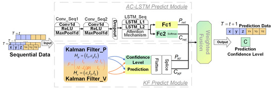
Figure 1.
AC-LSTM and KF composite model structure.
2.1. AC-LSTM Prediction Module
We implemented an AC-LSTM architecture for the network-prediction module. This hybrid model synergistically integrates convolutional neural networks (CNNs) and LSTM networks, leveraging the complementary strengths of both architectures. Specifically, the CNN component performs deep spatial feature extraction to capture trajectory motion patterns, whereas the LSTM module subsequently conducts temporal regression analysis on the processed sequential data. Compared with conventional LSTM implementations, our framework demonstrates a superior capability for modeling complex spatiotemporal relationships. To further enhance the representational power of the model, we incorporated an attention mechanism that dynamically prioritizes informative temporal states. The mathematical formulation of this architecture is described below.
For convolutional operations, we employed a parallelized one-dimensional convolution scheme that simultaneously processed multi-dimensional input features. This design enables the efficient extraction of spatial correlations across different trajectory parameters while maintaining temporal coherence. The convolution operation is mathematically expressed as follows:
where denotes the output of the convolutional sequence (specifically serving as the LSTM input when a single convolutional layer is deployed), represents the input feature vector at timestep t, , and denotes the learnable convolution kernel weights and bias term, respectively, with the ReLU serving as the nonlinear activation function.
In our LSTM network implementation, we employed a stacked multi-layer LSTM architecture to process sequential feature data. LSTM computational operations primarily consist of three fundamental gating mechanisms (forget gate, input gate, and output gate) coupled with dynamic cell-state updates. A detailed network schematic (Figure 2) and the corresponding mathematical formulation are systematically presented below.
where , , and represent the outputs of the forget, input, and output gates, respectively, and and denote the current cell state and hidden state, respectively.
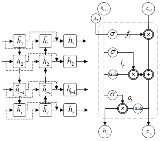
Figure 2.
LSTM Network Architecture and Unit Structure.
The forget gate regulates historical information retention through the following components: the sigmoid activation function governs the gate’s activation intensity, indicates the preceding hidden state, corresponds to the convolutional feature map from the previous timestep, and and are the trainable weight matrix and bias term, respectively. Output determines the proportion of the previous cell state information to be preserved.
The input gate modulates new feature integration via and as its parametric weights and bias, respectively, where the output specifies the assimilation rate of novel information into the current cell state.
The output gate manages the state visibility as follows: and constitute its learnable parameters, with the output scaling the contribution of the cell state to the updated hidden state.
Cell state updating combines gated operations from both the forget and input gates, utilizing the hyperbolic tangent (tanh) activation function to constrain state values within a predefined numerical range, where and parameterize the candidate state transformation. Subsequent hidden state generation depends on the refined cell state filtered through the output gate.
in the attention mechanism architecture, the query (Q), key (K), and value (V) vectors are derived through linear projections of the input embedding vectors (or outputs of the preceding layer) via distinct learnable weight matrices. The scaling factor , where denotes the dimensionality of the key vectors, is incorporated to regulate the magnitude the of dot product computations, thereby maintaining gradient stability during backpropagation. The attention weights were subsequently normalized using softmax activation to form a probabilistic distribution. The final network output synthesizes contextual dependencies across sequential positions through linear transformation parameters (, ) operating in the attention-modulated hidden state .
To enable the synchronous output of trajectory predictions and confidence estimates from the network prediction module, we implemented two task-specific fully connected branches in the output layer, one dedicated to trajectory regression and the other to confidence score estimation. The network training framework employs a multi-task learning paradigm in which distinct loss functions are strategically assigned to each subtask to ensure proper gradient flow during backpropagation [19,20]. This multi-objective optimization was formalized using a composite loss function:
where L represents the joint loss function, and and represent the loss functions for the regression tasks and confidence level assessment, respectively. The coefficient should be greater than to ensure the dominance of the regression task.
To enhance the initially defined confidence levels in the neural network module, we explicitly incorporated the confidence level estimation as a dedicated component of the network’s final output. Considering the distinctive characteristics of space targets—particularly their high velocity, long-range trajectories, and relatively low data noise—we adopted SNR as the classification criterion for confidence levels in the dataset. These predefined confidence levels were then used to train the confidence output layer of the network. The confidence level formulation for the AC-LSTM prediction module is expressed as
where k and C are the coefficients and biases of the sigmoid function, respectively, which were determined by empirically fitting different degrees of noise-added data from the training set.
2.2. KF Prediction Module
A two-channel Kalman filter prediction model was employed to mitigate the impact of fitting interference in the 3D space target trajectory data. This approach allows for the independent handling of the position and velocity data, thereby addressing the magnitude differences between these dimensions, which can impede accurate fitting. The state transition matrix F for both channels is initialized identically to ensure that the relationship between position and velocity remains consistent throughout the prediction process. The observation matrix H, employs distinct diagonal matrices to modify the mapping relationship between the position and velocity during the update process. The fundamental principles underlying the KF algorithm’s operational steps are summarized as follows [21].
here, and represent the system states before and after the update, respectively, while and denote the estimation error covariance matrices before and after the update, respectively, is the control input matrix, is the external control input, is the process noise covariance matrix, K is the Kalman gain coefficient, and is the measurement equation. These are all the process variables in the Kalman filter algorithm.
To further clarify the implementation details of the dual-channel Kalman filtering mechanism in this module, we provide the shared state transition matrix F and the distinct observation matrices corresponding to the two prediction channels. These matrices define the system dynamics and measurement relationships used in each filter branch. The specific forms are given as follows:
Here, represents a 3 × 3 identity matrix, is the discretization parameter. In the observation matrix, and denote the micro-coupling coefficients for position and velocity respectively. stands for the Jacobian matrix of acceleration with respect to position, which can be expressed as follows:
Here, the position vector is denoted as , represents the target acceleration, is the gravitational constant (taken as in this context), and r is the distance from the target to the origin.
The confidence metric of the KF prediction module follows a definition framework analogous to that of the AC-LSTM confidence formulation. The critical distinction stems from KF’s inherent stepwise recursive nature of KF: its prediction reliability quantification utilizes the accumulated multi-step forecast errors relative to ground truth observations. This error-driven confidence measure is mathematically expressed as follows:
where the position confidence and velocity confidence are defined as follows:
We employed linear and quadratic equations to model the position and velocity confidence metrics, respectively, where the coefficients and c represent the optimizable parameters of each corresponding regression function. The prediction uncertainty quantification is implemented through residual analysis over N steps, with and denoting the standard deviations of the position and velocity prediction residuals respectively, mathematically defined as
where are the measurement and prediction of step i and their residuals, respectively, and S is the standard deviation of the prediction residuals for a total of N steps.
2.3. Confidence-Based Fusion Module
In the fusion module, the predictions and confidence levels from the AC-LSTM and KF prediction modules were dynamically weighted to obtain the final 3D trajectory vector prediction result, P:
where and are the confidence levels of the two modules, and and are the prediction outputs from the AC-LSTM and KF modules, respectively. The final outputs are six-dimensional vectors consisting of the three-dimensional position and velocity coordinates.
Finally, the fused predicted trajectory, including both 3D position coordinates and 3D velocity vectors, was used as the model’s output, with a total weighted confidence score representing the reliability of the prediction result.
To summarize, the proposed framework incorporates noise-awareness at multiple levels to enhance robustness in uncertain environments. The AC-LSTM module leverages multi-task training on datasets with varying SNRs and utilizes a confidence-guided loss function to reflect prediction uncertainty. The Kalman filter module introduces a dual-channel linear filtering structure, where confidence is estimated through multi-step residual analysis. Finally, the fusion module adaptively integrates outputs from both branches based on their confidence levels, achieving a balanced and reliable prediction outcome even under significant noise, as demonstrated in the experiments presented in Section 4.
3. Simulated Dataset and Experimental Setup
This section serves as a supplement to the AC-LSTM and Kalman filter fusion framework proposed in Section 2. Rather than introducing a new method, it provides essential background and implementation details that support the development and evaluation of our approach. Specifically, we first present the physical principles and mathematical models used to simulate realistic three-dimensional space target trajectories, which form the basis of our custom dataset. We then describe the experimental environment, including both hardware and software configurations. Finally, we outline the hyperparameter optimization strategy employed for the AC-LSTM network and specify the final parameter settings adopted in the experiments. These elements are crucial for ensuring the reproducibility and reliability of the results reported in the subsequent sections.
Although physics-based models are well suited for generating idealized trajectory data under known conditions, they tend to be overly sensitive to measurement noise and environmental uncertainties, making them unsuitable for accurate real-time prediction. By contrast, the proposed data-driven framework—combining AC-LSTM with Kalman filter fusion—is designed to learn implicit motion patterns from historical data and offers enhanced robustness and predictive performance in uncertain and noisy scenarios. Unlike traditional motion models, the computational efficiency of neural network–based approaches is closely related to the number of neurons used. A detailed evaluation of the trade-off between computational time and prediction accuracy for our method is presented at the end of Section 5.
3.1. Simulated Space Target Trajectory Generation
As a fundamental trajectory model in high-speed aerospace vehicle dynamics, the minimum energy trajectory adheres to the physical principles governing the target motion and serves as a theoretical foundation for formulating advanced projectile trajectories. Therefore, this study employed trajectory data generated under the established model as the basis for systematic investigation. All simulated trajectories in the dataset follow the minimum energy principle. The principle is shown in Figure 3.
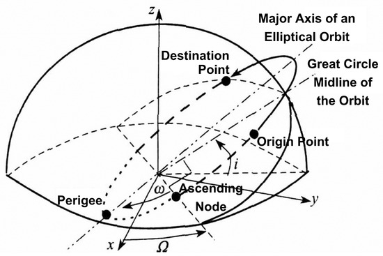
Figure 3.
Trajectory parameters in the principle of minimum energy trajectory.
Here, six parameters are used to define a complete space target trajectory: a is a semi-major axis; e is orbital eccentricity; i is orbital inclination; is the right ascension of the ascending node (RAAN); w is the argument of perigee; and is time of perigee passage.
Therefore, for a given launch point (geographic coordinates) and target points , a unique set of orbital parameters defines a complete minimum-energy trajectory. The mathematical representation is given by the following equation:
where , P, and E are functions related to (longitude) and (latitude), which have been extensively studied in the literature and will not be reiterated here. is the astronomical constant representing the Earth’s gravitational parameter, with a value of . and represent the major axis direction vector and the ascending node vector of the orbit, respectively. A, B, and C are the coefficients of the orbital plane equation . These coefficients are derived from the coordinates of the launch and target points transformed into the Earth-Centered Earth-Fixed (ECEF) coordinate system [22] and can be expressed as follows:
Here is the conversion relationship between geographic coordinates and ECEF coordinates:
Thus, by applying the minimum-energy trajectory model, a space target trajectory solution is obtained, and the complete coordinates of the trajectory are derived in the ECEF coordinate system. By discretely sampling the trajectory at fixed time intervals, the position and velocity of the space object at any given time along the trajectory can be determined as follows:
where and are the transformation vectors that define an orthogonal coordinate system in the orbital plane. The mathematical expressions for these vectors are as follows:
3.2. Network Hyperparameter and Dataset Parameters
To determine the optimal architectural hyperparameters of the network—including the convolutional layer depth, kernel dimensions, LSTM layer configuration, and hidden unit allocation—we implemented a systematic hyperparameter optimization framework. By leveraging GridSearchCV’s exhaustive search capability, we conducted a comprehensive grid-based hyperparameter search across predefined parameter spaces. The best-performing parameter configuration identified through this process was subsequently adopted as the final model specification. Figure 4 illustrates the operational workflow of the hyperparameter tuning methodology.
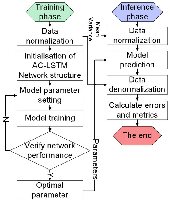
Figure 4.
Schematic Diagram of Network Hyperparameter Local Optimization.
The optimal network parameters are shown in the following Table 1.

Table 1.
Network parameter table.
The training datasets were generated through minimum-energy trajectory simulations, following the physical principles detailed in Section 3.1. Our simulation protocol involves the following: (1) discretizing the geographical constraints by sampling precise latitude-longitude coordinates within predefined launch and impact site boundaries, (2) computing three-dimensional space target trajectories for each coordinate pair, and (3) transforming all trajectory data into the ECEF coordinate system through rigorous coordinate conversion algorithms.
Our dataset construction protocol involved the strategic selection of 20 origin points, 20 designated destination points, and four apex points to generate 1600 distinct trajectories. To enhance data diversity and temporal resolution, we implemented an overlapping sliding window mechanism with a 10-step window length (corresponding to 10 s temporal coverage at 1 s sampling intervals) for trajectory segmentation. The complete parameter configurations governing the simulation framework are presented in Table 2.
Table 2.
Dataset parameter table.
To enhance the robustness and diversity of the dataset, we implemented controlled noise injection by introducing additive white Gaussian noise at varying amplitudes to the simulated trajectories. This procedure systematically generated data samples with predefined SNR levels ranging from 10 dB to 40 dB in 5 dB increments, thereby creating a comprehensive noise-resilient training corpus.
3.3. Experimental Environment
To ensure that the experimental control variables are the same, the experimental software and hardware configurations used in this study are listed in Table 3. All comparison models were run on the same platform.
Table 3.
Experimental environment table.
4. Performance Evaluation
4.1. Ablation Study on Model Components
To systematically validate the efficacy of our framework, we conducted a three-branch ablation study: (1) full architecture (AC-LSTM+KF)—the proposed confidence-based joint prediction algorithm; (2) AC-LSTM standalone—pure deep learning implementation without confidence-guided KF integration; and (3) KF standalone—the conventional filtering approach excluding neural network enhancements.
Through a comparative analysis of the prediction accuracy across different configurations, we further examined the synergistic role of AC-LSTM and the Kalman filter in trajectory prediction, highlighting the joint model’s advantages in handling both linear and nonlinear trajectories. The results of the ablation experiments are listed in Table 4.
Table 4.
Results of ablation experiments.
Ablation studies revealed distinct performance patterns across model configurations. The integrated AC-LSTM+KF architecture achieves superior precision, demonstrating an 82% improvement over standalone AC-LSTM and 96% enhancement compared to the KF-only implementation. This validates the complementary strengths: AC-LSTM’s nonlinear modeling capacity effectively captures complex trajectory patterns, whereas the KF’s linear estimation capability provides noise-resistant stabilization. This significant performance gap highlights the critical need for hybrid approaches in high-noise dynamic trajectory scenarios.
To validate the confidence estimation accuracy and training effectiveness of our neural component, we conducted isolated testing with pre-labeled confidence datasets. Figure 5 quantitatively compares the input confidence levels against network-derived confidence estimates across different noises, and the Spearman correlation coefficients (≤1) for the three dimensions of XYZ confidence are 0.987, 0.989, 0.990, respectively.
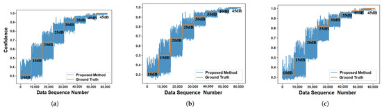
Figure 5.
Predicted confidence and ground-truth confidence. (a) Trajectory prediction confidence in the X dimension. (b) Trajectory prediction confidence in the Y dimension. (c) Trajectory prediction confidence in the Z dimension.
The Figure 5 demonstrates a comparison between the predicted and true confidence values in the network module. As shown, the predicted confidence varies inversely with data reliability and under low-SNR conditions, the confidence range expands significantly, indicating reduced reliability. Conversely, high-SNR scenarios yielded tightly clustered confidence values approaching 1.0, demonstrating consistency with statistical principles.
4.2. Prediction Accuracy Under Different SNR
To evaluate the efficacy and practical viability of our proposed methodology rigorously, we conducted comprehensive benchmarking against six established baseline approaches prior to controlled experimentation. The comparator models included the following: (1) a linear Kalman filter (KF), (2) a particle filter (PF) [23], (3) a multi-layer CNN, (4) LSTM, (5) a gated recurrent unit (GRU) [24], and (6) a transformer–encoder architecture [25].
All models were trained on identical input tensors with dimensions of 1 × 6 × 10, maintaining a consistent spatial–temporal resolution. Notably, conventional architectures generate output tensors of size 1 × 6 × 1, whereas our dual-branch framework produces enhanced 1 × 6 × 2 outputs through the channel-wise concatenation of prediction-confidence tensor pairs.
The simulation employed an identical methodology on test data with the following parameter configurations: origin point coordinates (125° W longitude, 45.0° N latitude, and 50 m altitude), destination point coordinates (115° E longitude, 35.0° N latitude, and 10 m altitude), and the trajectory apogee of 850 km. To simulate real-world sensing conditions, controlled Gaussian noise was injected at an SNR of 20 dB. The simulated test data are shown in Figure 6.
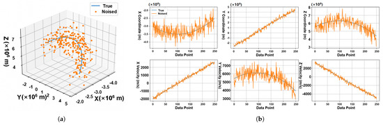
Figure 6.
3D trajectory and its decomposition diagram. (a) The 3D trajectory of the minimum energy trajectory and the coordinate sampling point after adding noise. (b) The components of the trajectory in the direction and velocity (ECEF coordinate system) and their noise sampling points.
Standard experimental protocols typically mandate noise reduction and signal filtering during data preprocessing to enhance algorithmic prediction accuracy. To rigorously evaluate the noise robustness of our method, we deliberately excluded preprocessing stages and directly utilized raw sensor data with 20 dB SNR for validation testing.
The benchmark evaluation measured three-dimensional trajectory prediction performance across comparative algorithms using mean absolute error (MAE) metrics. Our analysis specifically highlights both instantaneous error fluctuations and aggregate performance through mean error quantification, with comprehensive comparative results detailed in Figure 7.
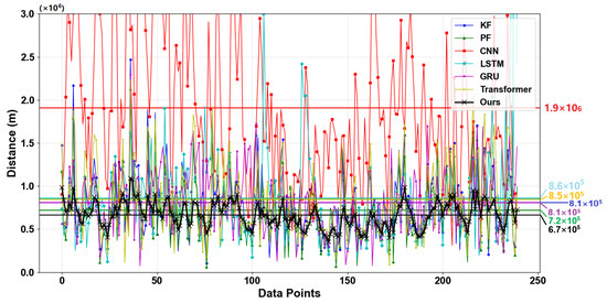
Figure 7.
Error performance of different models in 3D trajectory prediction.
The figure above illustrates the prediction error fluctuations of the proposed algorithm and comparison algorithms on the test data. The x-axis corresponds to the trajectory sampling points, and the y-axis quantifies the discrepancy between the predicted and true values. The colored markers along the y-axis display the overall mean errors for each of the seven algorithms.
As shown in the figure, the traditional convolutional neural network demonstrates limited efficacy in regressing high-speed aerospace trajectories in complex environments. In contrast, the proposed method exhibits a prediction error 2.8 times lower than that of conventional approaches. When configured with appropriate parameters, the baseline algorithms achieved relatively accurate predictions; however, our method showed statistically significant improvements: a 20.9% mean error reduction over Kalman filtering, 7.5% versus particle filtering, 28.3% against LSTM, 21% relative to GRU, and 26.9% compared to transformer architectures.
These experimental results conclusively demonstrate the dual advantage of the proposed algorithm for 3D trajectory prediction: optimal absolute accuracy coupled with minimal error fluctuations across operational scenarios.
To rigorously assess the noise robustness of the algorithm, we conducted comprehensive trajectory prediction experiments employing varying noise-corrupted datasets (10–40 dB SNR). The quantitative evaluation employed three complementary metrics: the MAE, root mean squared error (RMSE), and coefficient of determination (), systematically measuring precision loss, error magnitude, and model interpretability across signal degradation conditions. The experimental results are shown in Figure 8.
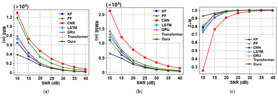
Figure 8.
Noise robustness characterization: prediction performance under signal degradation. (a) MAE values predicted via the algorithm at different SNRs. (b) RMSE values predicted via the algorithm at different SNRs. (c) index of the model at different SNRs.
Figure 8a,b show that the proposed algorithm consistently achieved the lowest MAE and RMSE values under different SNR conditions. In the experiment with an SNR of 10 dB, the prediction error metrics of the proposed algorithm were reduced by 38% and 41%, respectively, compared with the best-performing baseline algorithm. Figure 8c shows that the proposed algorithm achieved the highest value in the model evaluation. In the SNR experiment at 10 dB, the metric of the proposed algorithm is 13.6% higher than that of the best baseline model.
5. Comparison with Baseline Methods
The proposed confidence-aware fusion mechanism demonstrates superior prediction accuracy compared to conventional 3D trajectory predictors. Through the progressive refinement of prediction errors across trajectory phases, our method effectively integrates linear Kalman filtering with nonlinear neural dynamics. The baseline models used for comparison include both classical integration methods and recent deep learning approaches. Specifically, RK4 represents a physics-based baseline grounded in orbital motion equations, while DeepLSTM, CE-LSTM, and BiLSTM-AM are drawn from recent works targeting trajectory prediction under noisy conditions. These models provide diverse reference points for evaluating the effectiveness and robustness of the proposed hybrid AC-LSTM and Kalman filter framework.
The benchmark evaluation includes the following: (1) BiLSTM-AM networks; (2) CE-LSTM networks; (3) deep recurrent LSTM networks, with traditional trajectory equations as the reference baseline (based on four-order Runge-Kutta integration [26]). Experimental validation utilized the dataset described in Section 3.2, partitioned into 70% training, 20% validation, and 10% testing subsets.
Five metrics evaluate the prediction fidelity, with formal definitions provided as follows.
- Mean absolute error (MAE);MAE measures the mean absolute error between the predicted value and the actual value and is suitable for assessing the magnitude of the absolute error.
- Root mean square error (RMSE);RMSE measures the mean of the square root of the prediction error, which reflects the size of the prediction error, and larger errors are amplified.
- Mean absolute percentage error (MAPE);MAPE measures the prediction error as a percentage of the actual value and is often used to assess the relative error of the model, which can reflect the obvious scale differences in the data.
- Mean squared percentage error (MSPE);MSPE measures the squared error of the prediction as a percentage of the actual value and can penalize large errors, the value of which is sensitive.
- Coefficient of determination ();measures how well the model fits and how well the independent variable explains the dependent variable. The closer the r-squared value is to 1, the better the model. A value close to zero indicates a poor model fit.
Our experimental validation incorporates realistic noise simulation by introducing zero-mean Gaussian perturbations ( = 35,000 m, = 20,000 m, = 60,000 m) to the radar measurements, and the SNR of these data were calculated to be approximately 40 dB. Figure 9 and Table 5 compares the multi-dimensional prediction errors (X/Y/Z axes) and metrics of the five methods.
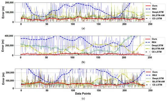
Figure 9.
Prediction error in three positional dimensions. (a) Prediction error in the X-axis direction. (b) Prediction error in the Y-axis direction. (c) Prediction error in the Z-axis direction.
Table 5.
The test metrics of the five algorithms are on the 3D trajectory dataset.
As shown in Figure 9 and Table 5, the proposed method demonstrates superior performance across all three spatial dimensions compared to the classical RK4 and several deep learning baselines (CE-LSTM, BiLSTM-AM, and Deep LSTM). Notably, in the Y-axis direction, which corresponds to the linear component of the trajectory, our method achieves a substantial performance advantage. Specifically, it records the lowest MAE (24,135 m), RMSE (30,813 m), and MAPE (0.93%) among all methods, indicating highly accurate and stable predictions. This significant improvement is attributed to the proposed model’s strong capability in capturing linear motion trends and effectively leveraging the temporal dependencies of the data.
It is also important to note that the MAPE and MSPE values for the Y-axis are generally higher across all models. This does not necessarily indicate poor model performance. Rather, the Y-axis component exhibits relatively small variation ranges (as shown in Figure 6b), which amplifies relative error metrics such as MAPE and MSPE. Consequently, even small absolute deviations can result in large percentage-based errors. Despite this, our method still achieves the lowest MAPE and MSPE in the Y direction, underscoring its superior performance and stability in modeling linear trajectories under challenging evaluation conditions.
In contrast, the X and Z axes exhibit more nonlinear and oscillatory behavior, making the prediction task more challenging. Even so, our method still outperforms all baseline models in these two directions. For instance, it achieves an MAE of 32,446 m and RMSE of 40,022 m in the X-axis, and 52,659 m and 66,397 m in the Z-axis, respectively. Although the performance margins in these directions are slightly narrower due to the inherent complexity of nonlinear trajectories, the proposed method consistently delivers the best results. This indicates that our model can generalize well across both linear and nonlinear dynamic patterns.
In terms of overall prediction quality, our method also exhibits the highest coefficient of determination (R2), exceeding 97.66% in all three directions and reaching up to 99.98% on the Y-axis, which confirms its strong goodness-of-fit. Moreover, the mean squared percentage error (MSPE) remains below 0.01% in all cases, showcasing the model’s remarkable robustness to noise. Taken together, the experimental results clearly validate that the proposed dual-confidence fusion model not only improves prediction accuracy across multiple dimensions but also enhances robustness under noisy conditions, thereby making it highly suitable for practical applications in 3D trajectory forecasting.
Table 6 provides a comparison of memory occupancy and reasoning efficiency across several methods. The results indicate that the traditional method, which relies on nested loops, exhibits a slower performance. Although the reasoning time for the method proposed in this study is marginally slower than that of other approaches, it incorporates a greater number of neurons, resulting in the highest reasoning efficiency among the evaluated methods.
Table 6.
Memory usage and inference efficiency of several methods.
6. Conclusions
The experimental results on a simulated three-dimensional space target dataset confirm that the proposed method not only achieves high prediction accuracy but also demonstrates exceptional robustness in complex environments. Specifically, our confidence-based dual-model fusion framework, which separately processes linear and nonlinear trajectory components, significantly improves the prediction performance. Compared to other related algorithms, our method reduces the prediction error in space target trajectory prediction, with the MAE value of the prediction error reduced by at least 11.1%, and the RMSE value was reduced by at least 12%. Furthermore, the proposed method maintains higher operational efficiency within the neural network module, ensuring that computational requirements are well balanced with performance gains. These results underscore the effectiveness of our dual-confidence fusion strategy, combining the strengths of the AC-LSTM network for nonlinear motion prediction and the Kalman Filter for quasi-linear motion modeling. This approach not only enhances prediction accuracy but also ensures reliability in real-world aerospace defense applications. The proposed method holds significant potential for aerospace defense systems, where rapid and precise target prediction is crucial for operational success in the complex and dynamic environments typical of aerospace missions.
Future work could explore several promising avenues: first is extending the model to address a broader range of defense scenarios, such as those encountered in aerospace environments, where rapid changes in target motion and diverse threat profiles are prevalent. By testing the model with different datasets, including real-world projectile trajectory data, we can enhance its generalizability and ensure its effectiveness in varying operational conditions encountered in aerospace defense. Second, investigating more advanced feature extraction techniques and confidence estimation methods will allow for further refinement of the model’s predictive accuracy, Which is critical for space situational awareness systems, where precision is paramount. Finally, integrating additional sensor data from sources such as radar, infrared, and satellite systems will strengthen the model’s robustness, providing a more comprehensive and adaptable solution for aerospace applications. These advancements would not only improve prediction accuracy but also ensure that the model can be effectively deployed in real-time aerospace missions, where quick, reliable, and accurate target tracking is vital for mission success.
Author Contributions
Conceptualization, C.W. and J.Z.; software, J.Z. and Y.W.; validation, J.Z. and Y.W.; formal analysis, C.W. and J.W.; resources, C.W.; writing, J.Z.; editing, Y.W. All authors have read and agreed to the published version of the manuscript.
Funding
This research was funded by the National Natural Science Foundation of China, grant number 61301211, and the China Scholarship Council, grant number 201906835017.
Data Availability Statement
All data presented in this paper were derived from our independently conducted simulations, and the complete dataset will be made publicly accessible in the near future.
Conflicts of Interest
The authors declare no conflicts of interest.
References
- Tang, C.Y.; Tang, J.; Zeng, M.J. Aircraft Flight Trajectory Prediction Based on Kalman Filtering. Mod. Inf. Technol. 2023, 16, 74–78. [Google Scholar]
- Chen, J.; Li, X.; Song, Y.S.; Dong, X.N. Real-time tracking of infrared dim-small target with multi-feature adaptive fusion under double confidence. J. Beijing Univ. Aeronaut. Astronaut. 2024, 1–13. [Google Scholar] [CrossRef]
- Liu, Y.; Zhang, M.N.; Liu, H.S. Moving object detection and tracking system based on FPGA. Integr. Circuits Embed. Syst. 2024, 24, 62–66. [Google Scholar]
- Zhang, Y.; Liu, Z.; Yang, D.; Wang, B.; Wang, Y. 3D Point Cloud Target-Tracking Algorithm Fusing Motion Prediction. J. Signal Process. 2023, 3, 516–523. [Google Scholar] [CrossRef]
- Nielsen, M. Deep Learning. Neural Network and Deep Learning. 2019. Available online: http://neuralnetworksanddeeplearning.com/ (accessed on 1 October 2024).
- Yu, Y.; Si, X.; Hu, C.; Zhang, J. A review of recurrent neural networks: LSTM cells and network architectures. Neural Comput. 2019, 31, 1235–1270. [Google Scholar] [CrossRef] [PubMed]
- Ji, R.; Zhang, C.; Liang, Y.; Wang, Y. Trajectory prediction of boost-phase ballistic missile based on LSTM. Syst. Eng. Electron. 2022, 44, 1968–1976. [Google Scholar] [CrossRef]
- Ren, J.; Wu, X.; Bo, Y.; Wu, P.; He, S. Ballistic Trajectory Prediction Based on Context-enhanced Long Short-Term Memory Network. Acta Armamentarii 2023, 44, 462–471. [Google Scholar]
- Liang, T.J.; Sun, K.; Fan, J.; Zheng, X.L.; Liao, R. Prediction of external ballistic trajectory and landing point of mortar based on BiLSTM-AM. J. Gun Launch Control 2024, 1–10. [Google Scholar] [CrossRef]
- Wu, Y. Design of Indoor 3D Tracking System Based on UWB. Integr. Circuits Embed. Syst. 2023, 23, 71–74. [Google Scholar]
- Chen, J.; Xiang, L.; Yan, M.; Guo, Y. Trajectory Tracking Based on BP Neural Network and Extended Kalman Filter. Comput. Simul. 2024, 41, 508–512. [Google Scholar]
- Dai, L.C.; Liu, X.; Zhang, H.Y.; Dai, X.; Wang, C.G. Flight target track prediction based on Kalman filter algorithm unfolding. Syst. Eng. Electron. 2023, 45, 1814–1820. [Google Scholar]
- Capobianco, S.; Millefiori, L.M.; Forti, N.; Braca, P.; Willett, P. Deep Learning Methods for Vessel Trajectory Prediction Based on Recurrent Neural Networks. IEEE Trans. Aerosp. Electron. Syst. 2021, 57, 4329–4346. [Google Scholar] [CrossRef]
- Lui, D.G.; Tartaglione, G.; Conti, F.; De Tommasi, G.; Santini, S. Long Short-Term Memory-Based Neural Networks for Missile Maneuvers Trajectories Prediction. IEEE Access 2023, 11, 30819–30831. [Google Scholar] [CrossRef]
- Jin, N.; Wu, J.; Ma, X.; Yan, K.; Mo, Y. Multi-Task Learning Model Based on Multi-Scale CNN and LSTM for Sentiment Classification. IEEE Access 2020, 8, 77060–77072. [Google Scholar] [CrossRef]
- Sener, O.; Koltun, V. Multi-Task Learning as Multi-Objective Optimization. Adv. Neural Inf. Process. Syst. 2018, 31. Available online: https://proceedings.neurips.cc/paper_files/paper/2018/hash/432aca3a1e345e339f35a30c8f65edce-Abstract.html (accessed on 10 October 2024).
- Xiao, B.; Guo, P.C.; Heng, J.; Zhang, C.Z. Solution and Simulation of Limited Energy Trajectory for Ballistic Missile. Syst. Simul. Technol. 2009, 5, 12–17. [Google Scholar]
- Livieris, I.E.; Pintelas, E.; Pintelas, P. A CNN–LSTM model for gold price time-series forecasting. Neural Comput. Appl. 2020, 32, 17351–17360. [Google Scholar] [CrossRef]
- Yang, P.; Zhao, P.; Zhou, J.; Gao, X. Confidence weighted multitask learning. Proc. Aaai Conf. Artif. Intell. 2019, 33, 5636–5643. [Google Scholar] [CrossRef][Green Version]
- Fernando, K.R.M.; Tsokos, C.P. Dynamically weighted balanced loss: Class imbalanced learning and confidence calibration of deep neural networks. IEEE Trans. Neural Netw. Learn. Syst. 2021, 33, 2940–2951. [Google Scholar] [CrossRef]
- Liu, D.; Zhao, Y.; Xu, B. Tracking Algorithms Aided by the Pose of Target. IEEE Access 2019, 7, 9627–9633. [Google Scholar] [CrossRef]
- Dong, Y.; He, Y.; Wang, G. A generalized least squares registration algorithm with Earth-centered Earth-fixed (ECEF) coordinate system. In Proceedings of the 2004 3rd International Conference on Computational Electromagnetics and Its Applications, Beijing, China, 1–4 November 2004; pp. 79–84. [Google Scholar]
- Daum, F.; Huang, J.; Noushin, A. Track before detect for radar using stochastic particle flow filters. In Proceedings of the 2020 IEEE Radar Conference (RadarConf20), Florence, Italy, 21–25 September 2020; pp. 1–6. [Google Scholar]
- Yang, Q.; Zhang, X.; Du, Y.; Zuo, Y. Radar Signal Modulation Recognition based on Multi-scale Self-correlation Combined with Layered Convolution-GRU Network. In Proceedings of the 2024 6th International Conference on Electronic Engineering and Informatics (EEI), Chongqing, China, 28–30 June 2024; pp. 1801–1804. [Google Scholar]
- Han, Y.; Huang, G.; Song, S.; Yang, L.; Wang, H.; Wang, Y. Dynamic neural networks: A survey. IEEE Trans. Pattern Anal. Mach. Intell. 2021, 44, 7436–7456. [Google Scholar] [CrossRef] [PubMed]
- Turacı, M.Ö.; Öziş, T. Derivation of three-derivative Runge-Kutta methods. Numer. Algor 2017, 74, 247–265. [Google Scholar] [CrossRef]


Disclaimer/Publisher’s Note: The statements, opinions and data contained in all publications are solely those of the individual author(s) and contributor(s) and not of MDPI and/or the editor(s). MDPI and/or the editor(s) disclaim responsibility for any injury to people or property resulting from any ideas, methods, instructions or products referred to in the content. |
© 2025 by the authors. Licensee MDPI, Basel, Switzerland. This article is an open access article distributed under the terms and conditions of the Creative Commons Attribution (CC BY) license (https://creativecommons.org/licenses/by/4.0/).