Abstract
This paper introduces the ProVANT Simulator, a comprehensive environment for developing and validating control algorithms for Unmanned Aerial Vehicles (UAVs). Built on the Gazebo physics engine and integrated with the Robot Operating System (ROS), it enables reliable Software-in-the-Loop (SIL) and Hardware-in-the-Loop (HIL) testing. Addressing key challenges such as modeling complex multi-body dynamics, simulating disturbances, and supporting real-time implementation, the framework features a modular architecture, an intuitive graphical interface, and versatile capabilities for modeling, control, and hardware validation. Case studies demonstrate its effectiveness across various UAV configurations, including quadrotors, tilt-rotors, and unmanned aerial manipulators, highlighting its applications in aggressive maneuvers, load transportation, and trajectory tracking under disturbances. Serving both academic research and industrial development, the ProVANT Simulator reduces prototyping costs, development time, and associated risks.
1. Introduction
The development of robotic systems has garnered significant attention due to their expanding range of applications. Robot design typically involves the integration of mechanical structures, hardware components, and software systems. During the development process, control hardware and software can be tested directly on the physical prototype. However, this approach carries substantial safety risks, including potential equipment damage and, in severe cases, injuries or fatalities. These risks are particularly critical in Unmanned Aerial Vehicles (UAVs), which often feature powerful actuators, fast-moving parts, and, in some instances, heavy payloads. Moreover, accidents during prototyping can significantly increase costs and extend development time, creating serious challenges for institutions and researchers with limited resources. In this context, system simulations offer a practical and cost-effective alternative. They support the development, validation, tuning, and optimization of advanced control strategies without the need for physical implementations, while also mitigating the risks associated with prototype failures.
Developing reliable control strategies and implementing them in hardware for robots involves addressing several inherent challenges, including meeting real-time execution requirements, debugging complex control code, handling high nonlinear dynamics with several degrees of freedom (DOF), and ensuring robustness. In light of these challenges, this paper introduces the ProVANT Simulator (The ProVANT Simulator can be accessed at https://github.com/ProVANT-Project/ProVANT_Simulator, along with its comprehensive User Manual.), a realistic and versatile simulation platform designed to support the development and validation of robotic control algorithms.
ProVANT is a collaborative project dedicated to the design and development of Unmanned Aerial Vehicles (UAVs). Initiated in 2013, it brings together two Brazilian universities—the Federal University of Minas Gerais and the Federal University of Santa Catarina—and international partners such as the University of Seville in Spain. The project encompasses various aspects of UAV development, including airframe design, electronic systems, and software, with particular emphasis on advanced control strategies.
The ProVANT Simulator supports Software-in-the-Loop (SIL) experiments, in which control strategies are executed on a general-purpose computer. This setup is particularly useful during the early stages of development, allowing for debugging and preliminary performance assessment in a controlled environment. However, SIL simulations do not always reflect the constraints of real-world deployment, as there are often significant differences in processing power, memory, and timing behavior between desktop workstations and the embedded platforms used in actual robots. To bridge this gap, the simulator also supports Hardware-in-the-Loop (HIL) experiments, enabling the control software to run directly on the target embedded hardware. This capability enables more accurate performance evaluation under realistic computational conditions, bringing the testing process closer to final deployment.
Although the simulator is primarily designed for advancing UAV technologies, its architecture is general enough to accommodate a wide range of robotic systems. The ProVANT Simulator is built on top of the Gazebo engine, leveraging its high-fidelity physics simulation, extensive library of sensors and actuators, and modular plug-in architecture. Gazebo is widely recognized for its realism and reliability and has been adopted by leading organizations such as the Defense Advanced Research Projects Agency (DARPA) (https://spectrum.ieee.org/darpa-robotics-challenge-simulation-software-open-source-robotics-foundation, accessed on 14 August 2025) and the National Aeronautics and Space Administration (NASA). It has also served as the simulation backbone for several high-profile research initiatives [1,2,3].
Designed to serve both academic research and industrial development, the ProVANT Simulator has been developed by experts in control and aerospace engineering to support a wide range of UAV platforms, including quadrotors, tilt-rotors, and unmanned aerial manipulators. It enables the simulation of complex tasks such as aggressive maneuvers, load transportation, and trajectory tracking across various flight modes—including helicopter, fixed-wing, and transitional phases in tilt-rotor configurations.
The main contributions of this work are twofold. First, we introduce the ProVANT Simulator, an open-source simulation platform released under the MIT license, designed to support the development, testing, and validation of robot control algorithms using visual feedback in both SIL and HIL configurations. Built on a modular architecture using the Robot Operating System (ROS) and Gazebo, it allows for seamless integration with external tools, real-time execution, and fosters reproducibility in experimental research. Second, we validate the simulator with case studies using advanced control strategies from peer-reviewed journals. The results not only confirm the correct implementation of these strategies but also demonstrate the simulator’s realism and effectiveness for high-fidelity UAV simulation and controller evaluation.
The remainder of this paper is structured as follows: Section 2 provides an overview of existing UAV simulation frameworks and highlights their key characteristics. Section 3 describes the main features of the ProVANT Simulator, including its software architecture and integration with widely used development tools. Section 4 presents a series of case studies that demonstrate the simulator’s versatility across various UAV configurations and application scenarios. Finally, Section 5 offers concluding remarks and outlines directions for future research.
2. Related Works
This section reviews key projects and studies on UAV simulation environment, highlighting their contributions, and positioning the ProVANT Simulator within this landscape.
In [4], a platform called AuRoRA has been described for the simulation of rotary-wing UAVs with support for HIL. It includes tools for comprehensive simulation, such as actuator modeling, mathematical representations, and sensor data acquisition from devices like Inertial Measurement Units (IMUs) and Global Positioning Systems (GPS). The platform supports distributed system simulations, facilitating the development of computationally intensive control strategies. However, it is not based on standardized technologies, making it difficult to extend to other UAV types and to incorporate new sensors. Additionally, the lack of visual feedback limits its ability to provide an intuitive representation of the simulation environment.
Similarly, RotorS [5] is a simulation project developed at ETH Zurich, focusing on aerial robots. It provides ready-to-use models for several multicopters and features the ability to accept commands and output sensor measurements via MAVLink messages [6]. However, as it is specifically designed for aerial robots, it lacks compatibility with other robots types. Moreover, it does not include functionalities for managing the simulation time step, which hinders the simulation of resource-intensive control strategies and results in limited computational performance.
In contrast to simulation-focused software like AuRoRA and RotorS, the main ROS distribution includes the ROS Control package [7], which provides tools for developing robot controllers. Widely used across robotics applications, ROS Control emphasizes high-performance controller development in C++, offering libraries and tools to create real-time controllers and implement common algorithms such as PID controllers. However, this package requires extensive knowledge of ROS and lacks support for higher-level programming languages like MATLAB. Additionally, it has a steep learning curve and demands advanced software development skills for effective use.
Recent surveys have provided further insights into UAV simulation tools, highlighting the available solutions and their targeted applications. For instance, ref. [8] has reviewed over forty UAV simulators, analyzing their benefits, shortcomings, and suitability for research and operational needs. Among these, Gazebo has been emphasized for its modularity and compatibility with robotic frameworks like ROS, making it a popular choice for academic research. FlightGear has been noted for its high-fidelity aerodynamics modeling, but it is less suited for rapid prototyping due to limited extensibility. Meanwhile, X-Plane has been recognized for its industrial-grade physics accuracy, though it comes with a steep learning curve and limited support for custom UAV configurations. The study has underscored important decision factors for selecting simulators, such as extensibility, real-time capabilities, ease of hardware, and computational requirements, providing researchers with guidelines for choosing tools tailored to their specific projects.
Expanding on this topic, ref. [9] has discussed UAV simulation frameworks, particularly focusing on their role in performance testing. It has identified key metrics such as computational load, simulation accuracy, and scalability as primary concerns for researchers. Tools like ArduPilot SITL and PX4 SITL have been highlighted for their integration with real autopilot systems, enabling realistic SIL simulations. The paper has also emphasized the importance of balancing computational efficiency with simulation fidelity, especially for applications requiring real-time performance, such as multi-UAV coordination and path planning algorithms.
In addition to general-purpose tools, specific application-oriented frameworks have been developed. For example, ref. [10] have demonstrated the adaptability of simulation platforms like Unreal Engine for specialized tasks. The paper has emphasized the integration of high-fidelity visualization and environmental modeling to validate UAV flight paths in landslide-prone regions. This approach not only enables realistic testing of flight plans but also provides valuable insights into UAV interactions with complex terrains.
Another notable work, ref. [11], has categorized simulation tools based on their capabilities for testing and validating UAV performance. It has underscored the importance of simulation testbeds for evaluating control algorithms, sensor integration, and mission planning within controlled environments. The paper has highlighted how platforms such as Simulink and Gazebo can be extended to support diverse UAV configurations and facilitate the development of advanced control strategies.
While these tools and frameworks have made significant contributions, many lack comprehensive features such as modularity, support for multiple robots configurations, and seamless integration with real-time systems. The ProVANT Simulator, introduced in this manuscript, addresses these limitations by offering a user-friendly, flexible, and robust environment that combines SIL and HIL simulations within an intuitive graphical interface. To summarize and facilitate comparison of the main UAV simulation platforms reviewed in this section and the ProVANT Simulator, Table 1 presents the most relevant characteristics. The architecture of the ProVANT Simulator is detailed in the following sections.

Table 1.
Feature comparison between the ProVANT Simulator and the presented related works.
3. ProVANT Simulator Overview
This section outlines the key features of the developed ProVANT Simulator, emphasizing those most relevant to its primary users, including researchers and developers working on UAV control strategies. A key objective in the development of the ProVANT Simulator was to leverage existing open-source tools and widely adopted standards. This is intended to maximize software reuse, minimize development effort, and ensure interoperability with established frameworks.
Rather than building the simulator from scratch, we based its implementation on the Gazebo platform [12]. Beyond the reasons mentioned in the Introduction, Gazebo was chosen because it meets specific functional requirements for UAV control development. These include providing real-time visual feedback, enabling the construction of complex and dynamic simulation environments, and supporting interactive manipulation of objects and scenarios. Gazebo also offers a rich library of built-in sensors, compatibility with standard robot description formats such as Unified Robot Description Format (URDF) and Simulation Description Format (SDF), and a modular, plugin-based architecture that facilitates extensibility. Furthermore, its native integration with ROS [13] allows for efficient communication between components via ROS topics, supporting asynchronous and event-driven interactions across distributed nodes. Figure 1 presents an overview of the adopted software architecture.
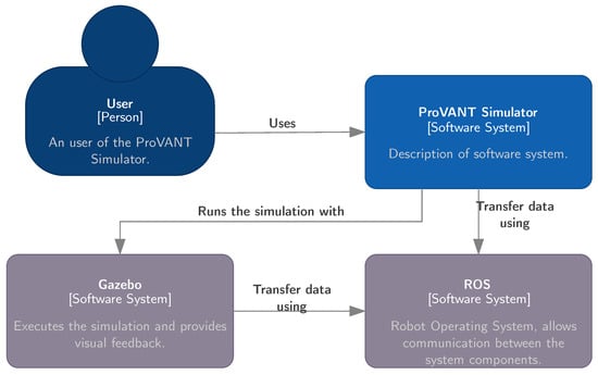
Figure 1.
Overview of the ProVANT Simulator software architecture.
3.1. Simulator Internal Structure
Figure 2 illustrates the internal elements of the ProVANT Simulator, which are represented as containers—modules composed of multiples components. In addition to these software elements, the ProVANT Simulator also includes ready-to-use UAV descriptions, equipped with plugins for state vector measurements and actuator simulation. Figure 2 also highlights the Sensor and Actuator plugin components, which extend Gazebo’s functionalities and provide essential interfaces for developing control strategies.
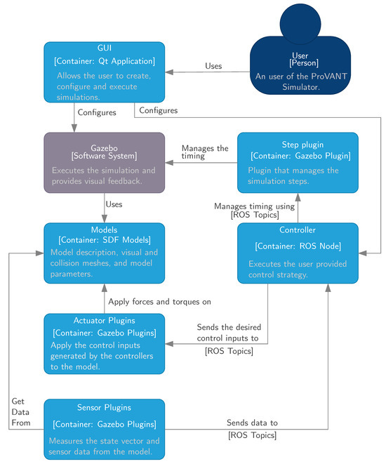
Figure 2.
Containers representing the internal elements of the ProVANT Simulator.
The Step plugin (located at the top-right portion of Figure 2) is a container that replaces the Gazebo’s standard timing management mechanism, allowing the controller to manage simulation timing. This plugin ensures that the simulation advances only after the control strategy has completed all computations for the current step, regardless of the processing time required.
The GUI container (located on the top-left portion of Figure 2) is designed to simplify simulation setup and debugging. It enables users to create, configure, and execute simulations without relying on the standard command-line tools from ROS and Linux, significantly lowering the learning curve for using the simulator and developing new scenarios. Additionally, the GUI includes features to streamline the creation and compilation of control strategies, as well as tools for inspecting the sensors and actuators available on each robot.
The Models container (located on the middle-left of Figure 2) encompasses all robot descriptions, including their visual and collision meshes, physical parameters, and configuration files. Defined using SDF, these models may incorporate aerodynamic plugins and simulate external disturbances.
The Controller container encompasses all essential functionalities for communication, storage of the simulation results, timing management, and other requirements for executing the control strategies. Figure 3 presents a detailed view of this container, highlighting the user-provided control strategy (bottom) and the data logger component (top), which records simulation data for future analysis.
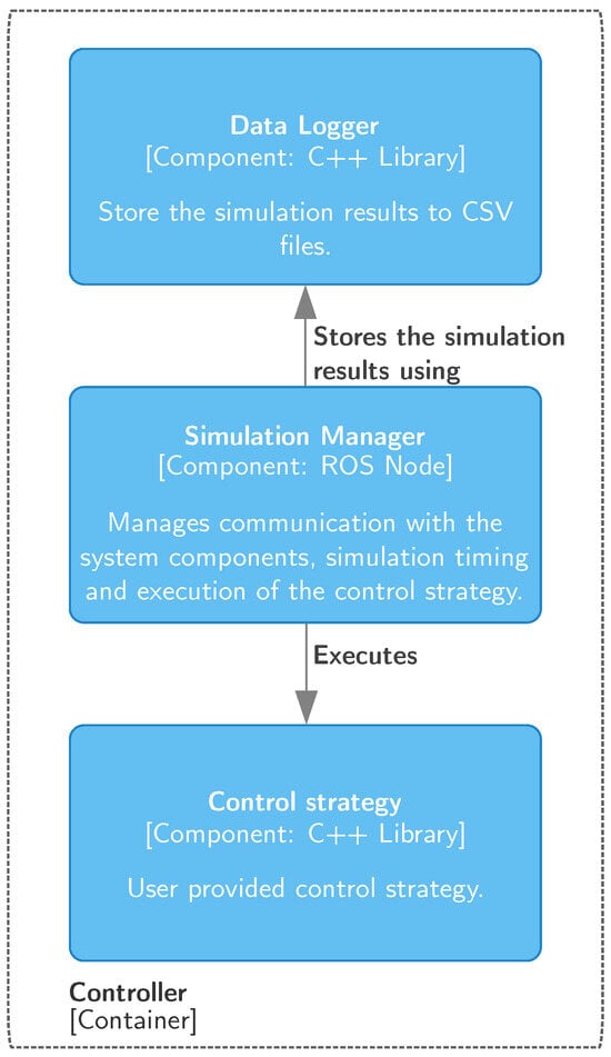
Figure 3.
Internal elements of the Controller container.
The Simulation Manager component, illustrated in Figure 3, is responsible for managing simulation timing and coordinating data exchange among system components, thereby ensuring consistent and reproducible execution of experiments in both SIL and HIL configurations.
The Data Logger component enables the ProVANT Simulator to export the simulation data generated to an external file in CSV format. This feature is particularly useful because the resulting file can be imported into external tools such as MATLAB and other similar software for further analysis and visualization, allowing for a detailed assessment of UAV performance during the simulation.
Figure 4 presents the class diagram of the Control Strategy component, which must be implemented by the user when designing a custom control strategy. This implementation is required only if the user wishes to develop a new control strategy. The following methods must be implemented:
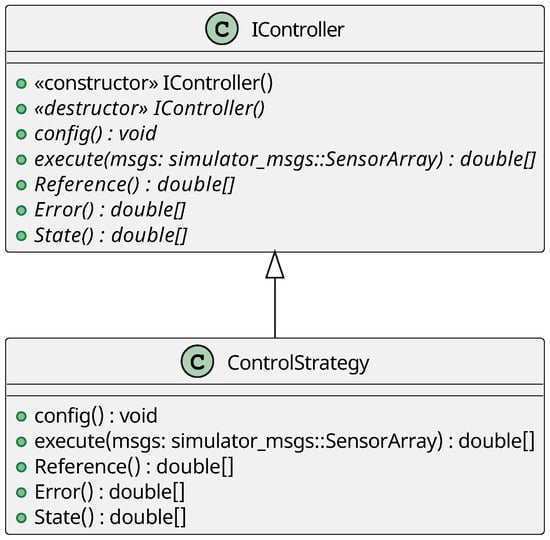
Figure 4.
Control strategy UML class diagram.
- Config(): This method is called once during the controller’s configuration phase, before the simulation starts. It is responsible for setting up all parameters required for the control strategy, such as defining gain values, initializing integrators, and preparing other necessary resources.
- Execute(): This method is called at every control step, receiving as a parameter a vector of sensor readings from the current UAV. It computes and generates a vector of control inputs to be applied to the robot, implementing the control law.
- Reference(): Returns the current reference vector of trajectory values to be tracked by the UAV.
- Error(): Returns the current error vector of the UAV’s states.
- State(): Returns the current UAV state vector.
3.2. Graphical User Interface
The GUI of the ProVANT Simulator provides an intuitive and streamlined environment for setting up, configuring, and executing robot simulations. Through this interface, users can manage simulation scenarios, vehicle models, and control strategies efficiently (A detailed explanation of the simulation workflow and graphical interface is available at https://github.com/ProVANT-Project/ProVANT_Simulator/blob/main/user_manual/Manual_ProVANT_Simulator.pdf).
The main window of the GUI is shown in Figure 5, which includes: (1) a hierarchical tree for configuring robot and simulation parameters, such as gravity settings, physics engine selection (e.g., ODE, Bullet, DART, Simbody), robot name, and initial pose. By double-clicking specific fields, users can edit these parameters or access additional configuration tabs for the model, world, controller, sensors, and actuators; (2) a preview panel displaying the selected robot model; (3) a preview of the simulation environment (world); and (4) a button to launch the Gazebo simulator. Robot models are selected through the Edit option in the top menu.
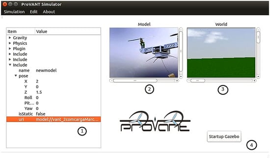
Figure 5.
Graphical user interface–main window.
By double-clicking the model entry in the tree structure highlighted in orange (1) (see Figure 5), the Controller tab is opened, as illustrated in Figure 6. Within this tab, users can: (1) select an existing control strategy; (2) create a new one; (3) open and edit an existing strategy; and (4) compile the selected controller. The tab also includes fields to configure (5) the sampling time and to define file paths for (6) tracking error, (7) reference signals, (8) sensor data, and (9) actuator data, facilitating post-analysis of the results. Button (10) confirms and saves the configuration. Still within the Controller tab, users can access the Sensors and Actuators tabs to configure the respective topics. These topics define the ROS interfaces through which the controller will communicate with the simulated system during execution.
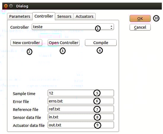
Figure 6.
Graphical user interface–Controller tab.
3.3. Simulation Modes
The ProVANT Simulator supports both synchronous and asynchronous execution modes in SIL and HIL simulations. While this flexibility benefits both configurations, asynchronous execution is particularly relevant in the HIL context, where additional hardware constraints and communication complexity arise due to the involvement of external embedded systems.
In the asynchronous HIL mode, controllers are validated under conditions compatible with real-time execution, making it suitable for implementations that must comply with strict timing constraints. In this configuration, the embedded system and the simulator operate independently, as shown in Figure 7. The corresponding plugin initializes the HIL Server task, which manages serial communication with the embedded computer. Upon receiving a request, the server either sends the current system state to the embedded device or receives and applies a control signal. Notably, Gazebo’s built-in Real-Time System scheduler is enabled to maintain a real-time factor (RTF) of , ensuring one second of simulation time equals one second of wall-clock time. The simulator advances continuously, sustaining the last received control input until it is updated by the HIL Server.
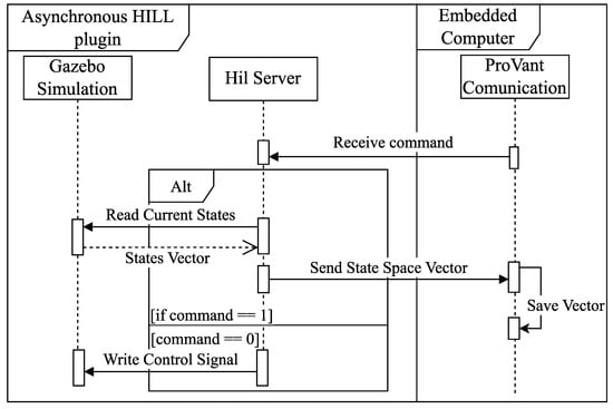
Figure 7.
General structure of asynchronous HIL mode.
In synchronous HIL mode, which is most appropriate to be used when the embedded system cannot compute the control signal within the system’s sampling time, the simulator assumes the role of master, and the embedded device operates as a slave. As depicted in Figure 8, the HIL plugin initializes a server that transmits the current state vector to the embedded computer and waits for the corresponding control signal. The simulation pauses during this exchange, resuming only after the control signal is received and applied.
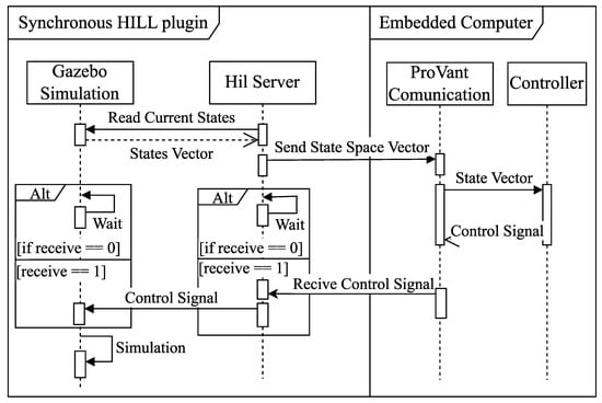
Figure 8.
General structure of the synchronous HIL mode.
3.4. Database of UAV Models
The ProVANT Simulator offers a diverse set of UAV models, providing users with a flexible foundation for various applications. The available models include:
- Quadrotor UAV;
- Unmanned aerial manipulator;
- ProVANT UAV 2 (with and without an external load);
- ProVANT UAV 3;
- ProVANT-EMERGENTIA UAV;
- VERSATILE UAV.
These models come equipped with fully configured components, including sensors and actuators, allowing users to focus on developing and testing control strategies rather than building models from scratch. The next section provides further details on these UAV models. It is worth highlighting that the UAV models used within the simulator are derived from CAD-based designs imported directly from CAD software. Consequently, their exact dynamical mathematical models are not known. This deliberate design choice enables the simulator to function as a crucial tool for validating mathematical models of UAV dynamics under realistic disturbances and uncertainties, in addition to its role as a development platform.
4. Case Studies
This section presents various case studies conducted using the ProVANT Simulator across different UAV models and experimental scenarios. The objective is to thoroughly explore and evaluate the capabilities of the simulator
4.1. Quadrotor UAV in an Urban Environment
This subsection presents a case study in which a quadrotor UAV navigates through an unknown 3D environment, conducted using the ProVANT Simulator. The objective is to evaluate the Nonlinear Model Predictive Control (NMPC) strategy and the obstacle detection algorithms proposed in [14] through SIL experiment. Further details of the quadrotor’s dynamic model can be found in [15].
The simulation was carried out on a computer running Ubuntu 20.04, equipped with an AMD Ryzen 7 3700U processor (1.51 GHz, 4 cores, 8 threads—AMD, Santa Clara, CA, USA) and 20 GB of RAM. The UAV parameters are presented in Table 2. The control system was implemented in MATLAB R2017a with the CasADi toolbox [16].
Table 2.
Parameters of the Quadrotor UAV.
To integrate the MATLAB-based control system with the ProVANT Simulator, the MATLAB Engine API for C++ was used. This interface allows the C++ controller to invoke an NMPC algorithm implemented in MATLAB by passing system states and sensor data as inputs. The computed control signals are returned and applied as thrust forces on the quadrotor. Figure 9 illustrates the data flow during this process.
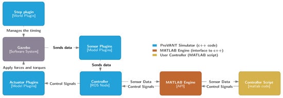
Figure 9.
Diagram of the ProVANT Simulator execution and flow of data using a controller written in MATLAB R2024b script using the MATLAB Engine API for C++.
During the experiment, the ProVANT Simulator provides the system states at each sample time, including the vehicle’s position, attitude, and linear and angular velocities. Additionally, a 3D LIDAR sensor is emulated within the ProVANT Simulator, supplying data about the environment. Both the system states and the LIDAR data are fed into the controller, which is executed on MATLAB R2024b and uses optimization techniques to compute the desired thrust forces for the rotors. These control inputs are then sent back to the ProVANT Simulator, which updates the rotor thrusts at each sample time.
The NMPC was designed to steer the quadrotor from an initial position to a desired target in minimum time while avoiding obstacles. Environment obstacles detected via the emulated LIDAR sensor were represented as polyhedra using a half-space representation. Obstacle-free zones were decomposed into convex subregions, which served to define constraints in the NMPC optimization problem, which aimed to minimize control effort while ensuring the vehicle remained within the feasible regions defined by the sensor data. Figure 10 shows the block diagram of the control system utilized in the SIL experiment. The NMPC control strategy is computationally demanding and does not meet real-time execution requirements. As a result, the simulation is performed in synchronous mode, allowing the control strategy to be tested while deferring computational optimization to future work. No external disturbances were considered in this case study.
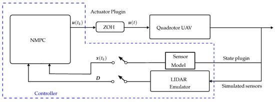
Figure 10.
Block diagram illustrating the NMPC control strategy utilized in the SIL experiment.
A video of the simulation is available at https://youtu.be/gkPfKWQnCU0. Figure 11 illustrates the quadrotor’s trajectory during the SIL experiment. Figure 12 and Figure 13 show the evolution of the position, linear velocities, attitude, and angular time derivatives, and Figure 14 shows the applied control signals during the SIL experiment. As can be observed, the quadrotor successfully navigated around three obstacles in an unknown environment while maintaining a safe distance, demonstrating the effectiveness of the NMPC strategy and the capabilities of the ProVANT Simulator in simulating complex control scenarios.
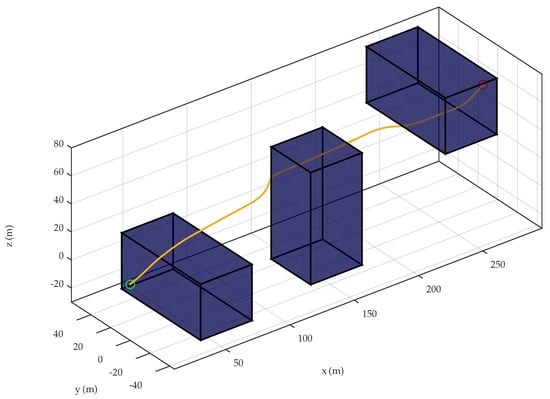
Figure 11.
Three-dimensional view of the trajectory (yellow line) traversed by the quadrotor UAV while avoiding three obstacles in an urban-like environment. The green and red circles correspond to the initial position of the quadrotor UAV and the desired target, respectively. This result corresponds to the case study in Section 4.1.
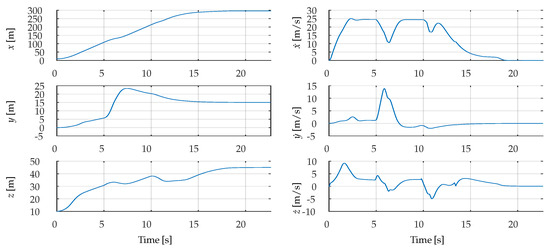
Figure 12.
Time evolution of the UAV’s position (x, y, z) and linear velocities (, , ) obtained from the SIL experiment.
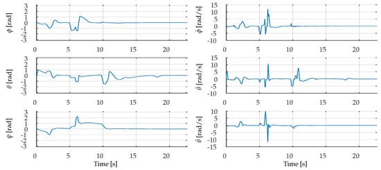
Figure 13.
Time evolution of the UAV’s attitude angles roll () pitch () and yaw () expressed in Euler angles using the ZYX convention about local axes, and their time derivatives (, , ) obtained from the SIL experiment.
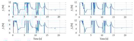
Figure 14.
Time evolution of the thrust forces applied to the quadrotor UAV rotors during the SIL experiment.
4.2. Quadrotor UAV for Aggressive Maneuvers
The primary objective of this section is to evaluate NMPC schemes proposed for aggressive motion control of a quadrotor UAV, using SIL experiments conducted in the ProVANT Simulator. The mathematical modeling and the NMPC control design are described in detail in [17]. A block diagram of the implemented control architecture is presented in Figure 15. The UAV parameters are detailed in Table 2.
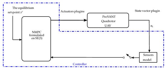
Figure 15.
Block diagram of the NMPC scheme implemented for the ProVANT quadrotor UAV to enable aggressive maneuvering.
As mentioned in the previous subsection, the NMPC control strategy is computationally demanding and does not meet real-time execution requirements. Accordingly, the simulation is performed in synchronous mode, allowing the control strategy to be tested while deferring computational optimization to future work. The SIL experiments were conducted on a general-purpose computer equipped with an Intel Core i7-4500U processor (1.8 GHz) featuring two physical cores and four logical threads, 8 GB of RAM, and an NVIDIA GT 750M GPU. The system ran on Ubuntu Linux version 18.04. No external disturbances are also considered in this case study.
The NMPC controllers are formulated on the manifold, enabling a global and unique representation of the vehicle’s motion. This singularity-free formulation proved advantageous during the experiments, as the quadrotor UAV successfully recovered from an upside-down configuration without the need for additional controllers or optimization layers, as illustrated in Figure 16. A video of the simulations is available at https://youtu.be/rEJB7pTyTB8, and the corresponding results are presented in Figure 17, Figure 18 and Figure 19.
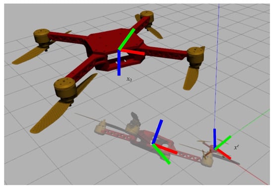
Figure 16.
Quadrotor UAV successfully recovering from an upside-down configuration.
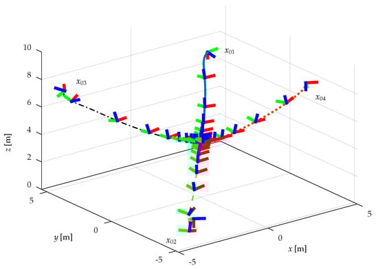
Figure 17.
3D visualization of the quadrotor UAV performing aggressive maneuvers under SIL simulation. The UAV is represented by a body-fixed reference frame, with axes colored as follows: red for the x-axis, green for the y-axis, and blue for the z-axis. The trajectories correspond to different initial conditions, labeled as , , , and . This result corresponds to the case study in Section 4.2.
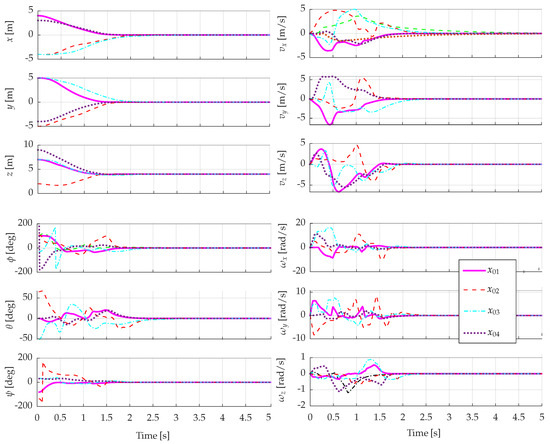
Figure 18.
Translational positions (x, y, z), attitude angles roll (), pitch (), and yaw () expressed in Euler angles using the ZYX convention about the local axes and their time derivatives, along with the linear velocities, obtained from the SIL experiment. This result corresponds to the case study in Section 4.2.
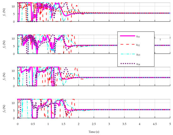
Figure 19.
Measured UAV propeller thrusts during aggressive motion control. The results confirm that the NMPC controller ensures compliance with the actuator limits, bounded between 0 and 12.3 N. This result corresponds to the case study in Section 4.2.
The experiment focused on point-to-point maneuvers, where the vehicle was guided from distinct initial configurations to a designated equilibrium set-point. The performance of the NMPC schemes was evaluated across four different initial conditions. In all cases, the controller successfully guided the system to the target equilibrium. The formulation on SE(3) effectively handled the singularities and discontinuities typically associated with Euler-angle representations. The ProVANT Simulator facilitated the initial tuning and thorough validation of the control strategy. Moreover, the controller consistently enforced the force constraints on the propellers, maintaining the applied thrust within the specified limits of 0 to 12.3 N, as illustrated in Figure 19.
4.3. Unmanned Aerial Manipulator
This section presents a case study using the ProVANT Simulator to conduct a HIL experiment on an Unmanned Aerial Manipulator (UAM), a system composed of a quadrotor UAV serially connected to a 3 DOF manipulator arm, as illustrated in Figure 20. The objective of the experiment was to tune, evaluate the real-time performance, and compare the nonlinear and control strategies. For a detailed description of the system modeling and control design, the reader is referred to [18]. The physical parameters of the UAM are listed in Table 3.
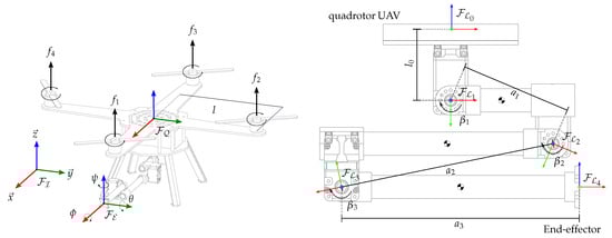
Figure 20.
The UAM mechanical design. In the illustration, () represent the forces generated by each propeller, while () denote the angular positions of the servo motors. The distances between joint axes are indicated by (); l represents the distance from the UAV’s origin to each propeller; is the distance from the UAV’s origin to the center of the first manipulator joint; (x, y, z) correspond to the translational positions, and () denote the end-effector’s orientation using Euler angles with a ZYX rotation sequence about the local axes.
Table 3.
Parameters of the unmanned aerial manipulator.
To emulate the grasping action, a custom Gazebo plugin was developed to simulate the behavior of an electromagnet. This plugin generates a virtual magnetic field capable of attracting and holding metallic objects when they are in close proximity. It continuously monitors the distance between the end-effector and the target object, and once the simulated end-effector reaches a predefined threshold, which was set to 1 mm in this experiment, the object is rigidly attached to the end-effector and treated as an additional load in the UAM structure. In addition to this grasping mechanism, the simulator includes plugins that model the aerodynamic ground effect produced by the UAV’s propellers, as well as friction forces acting on the manipulator’s joints, which are assumed disturbances for control design purposes.
Figure 21 shows the hardware components of the HIL framework and their connections, while Figure 22 shows the block diagram of the implemented software. The experiment was executed in asynchronous mode. The simulation server used in this case study is a general-purpose notebook computer equipped with an Intel Core i7 7500U processor, with two physical and four logical cores, running at 2.9 GHz, 16 GB of RAM, and a NVIDIA 920MX GPU. This computer runs the Ubuntu version 20.04 operational system and executes the software components of the ProVANT Simulator. The embedded system executes the software components of the controller, which is composed of a Raspberry Pi 3B+ SOC with a quadcore ARM Cortex-A53 processor running at 1.2 GHz, with 1 GB of RAM, and a VideoCore IV GPU. The embedded system and the simulation server communicate through a Local Area Network (LAN) connected by a 1 Gbps Ethernet switch, with fixed IP addresses 192.168.0.10 and 192.168.0.100, respectively. The controller is a ROS node implemented in the C++ programming language on the embedded system that communicates using ROS messages with the ProVANT Simulator. Gazebo was set up with the Open Dynamics Engine (ODE), considering a step time of 4 ms, and the controllers were executed with a sample time of 12 ms.
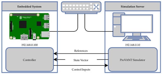
Figure 21.
Connection between the embedded system and the simulation server, the software running in each system component, and the data transmitted between the software.
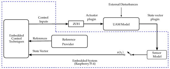
Figure 22.
Block diagram illustrating the control strategies implemented for the UAM during the HIL experiments.
Two experiments were conducted, experiment A and B, each with distinct objectives. A video recording of the experiments is available in https://youtu.be/t1t6xB98pJ4.
Experiment A, adapted from the benchmark proposed in [19], was conducted in a simplified environment to facilitate the tuning of the control laws according to a specific performance index, enabling a clearer comparison between the nonlinear and controllers. In this experiment, ground effect and joint friction forces of the manipulator are neglected, since they represent unmodeled dynamics for the controllers.
The scenario for Experiment A is shown in Figure 23. The task consists of a sequence of five phases: the UAM starts at the origin, m, then lifts off to m, and proceeds to m. Next, it reaches the final target while fully extending its manipulator arm at m. Finally, it returns to m. The experiments parameters are based on Table V of [19], with m, m, and m.
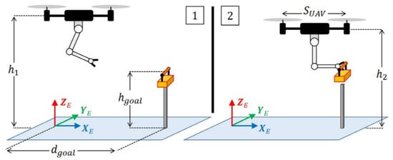
Figure 23.
Environment of the Experiment A. Image obtained from [19].
In contrast, Experiment B was designed to evaluate the controllers in a more realistic and challenging scenario, involving tasks commonly performed by UAMs. Additionally, it incorporates a plugin to emulate a northeasterly wind disturbance, applying N drag force to the center of gravity of the quadrotor UAV when operating outdoors (on the right side of the simulation environment). Experiment B aims to evaluate the following aspects of the UAM’s performance: (i) stable hovering capability; (ii) ability to follow a time-varying trajectory, grasp, and transport an object; (iii) dynamic response under manipulator arm movements; and (iv) robustness to disturbances such as ground effect, environmental wind, joint friction, and both parametric and structural uncertainties.
Figure 24 illustrates the simulation environment for Experiment B, indicating the UAM initial position, a static obstacle to be avoided, and a yellow metallic cube representing the target object. In this experiment, the UAM performs a mission composed of several phases, as illustrated in the Figure 25: the UAM starts from the initial position m, displaced from the first way point m, with all other states initialized to zero; goes through the intermediate point m; proceeds to the target position m where it hovers and fully extends its manipulator arm; it grasps a 200 g metallic cube; retracts the manipulator; returns to the starting position while carrying the object; and completes the mission with a landing.
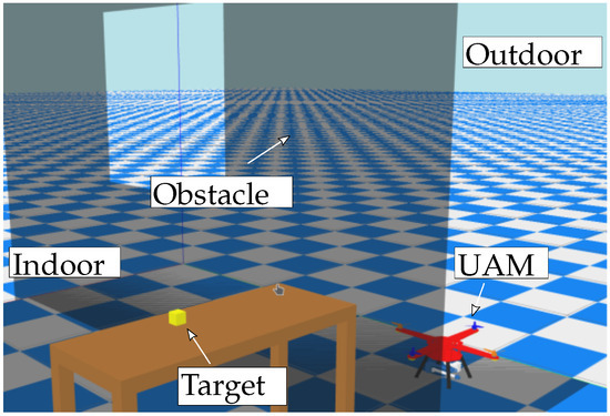
Figure 24.
Simulation environment designed in Gazebo for Experiment B.
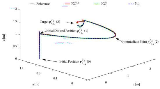
Figure 25.
3D trajectory of UAM end-effector during the HIL experiment. The red triangle indicates the point where the control failed and the UAM falls to the ground.
The position, velocity and acceleration references used in all experiments were generated offline using a modified version of the Rapidly-exploring Random Tree (RRT*) algorithm [20]. This planning algorithm was executed through MoveIt (MoveIt 1.0 is a ROS-Based framework that provides access to various motion planning algorithms and essential functionalities such as collision detection [21]), a ROS application designed for robotic motion planning. The resulting reference trajectories were exported to a CSV file and subsequently used during the simulation runs. The values observed during the HIL experiments of the UAM DOFs, control efforts, and of the control execution times are, respectively, shown in Figure 26, Figure 27 and Figure 28.
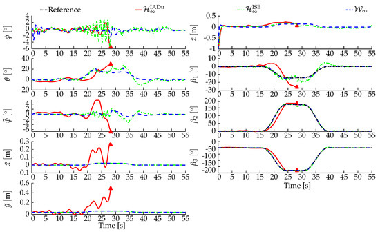
Figure 26.
Roll () and pitch () angles, error of the yaw () angle, error of the translational positions () and angles of the manipulator arm () during the HIL experiment. The red triangle indicates the point where the control failed and the UAM falls to the ground. This result corresponds to the case study in Section 4.3.
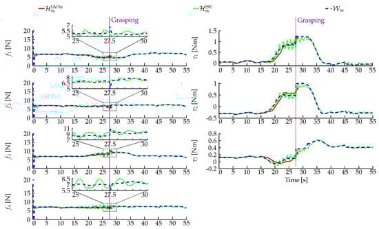
Figure 27.
Applied control inputs during the HIL experiment. The purple line indicates the approximate instant in which the cube is grasped by the end-effector using the different controllers, and the red triangle indicates the point where the control failed and the UAM falls to the ground. This result corresponds to the case study in Section 4.3.
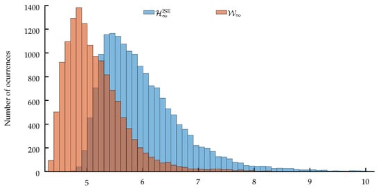
Figure 28.
Control law execution time for the case study in Section 4.3.
In this case study, the ProVANT Simulator has demonstrated its value beyond serving as a platform for testing real-time performance of control strategies in complex systems through HIL experiments. It proved capable of emulating realistic operating conditions, enabling comprehensive evaluation of controller robustness. Moreover, it facilitated comparative analyses between different control strategies, supporting control engineers in selecting the most suitable approach to achieve specific performance goals.
4.4. ProVANT UAV 2 for Load Transportation
This section presents case studies involving the ProVANT UAV 2, a tilt-rotor unmanned aerial vehicle designed to perform load transportation missions, as illustrated in Figure 29. This UAV can be modeled as a mechanical system composed of four key rigid bodies: (i) the main UAV body, which includes batteries, electronics, ABS structure, and landing gear; (ii) the right thruster group, consisting of the right thruster and a revolute joint; (iii) the left thruster group, comprising the left thruster and a revolute joint; and (iv) the suspended load group, which includes the payload and the cable. Table 4 presents the physical parameters employed in the ProVANT Simulator. The following modeling assumptions are considered:
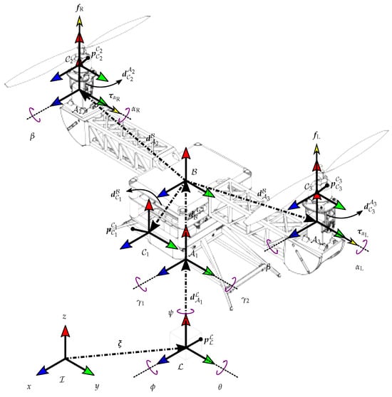
Figure 29.
The ProVANT UAV 2 mechanical design.
Table 4.
Parameters of the ProVANT UAV 2 with suspended load.
- The cable is rigid and massless.
- The center of mass of the main body does not align with the aircraft’s geometric center.
- The attachment point of the cable is offset from both the main body’s geometric center and center of mass.
- The centers of mass of the thruster groups are displaced from their respective tilting axes.
4.4.1. Trajectory Tracking of the Load with State Estimation
We first describe a case study involving load transportation by the ProVANT UAV 2, focusing on robust trajectory tracking of the suspended load while stabilizing the tilt-rotor UAV. The desired load trajectory, denoted as , comprises various connected paths, including vertical take-off in spiral, lateral and longitudinal flight under exogenous forces, and landing, as detailed in Table 5. For a detailed description of the control strategy and theoretical formulation, the reader is referred to [22].
Table 5.
Paths that compose the trajectory to be tracked by the load.
In this case study, the state variables are estimated using data from multiple simulated sensors mounted on the UAV, each operating at distinct sampling rates. These include a GPS, barometer, IMU, camera, and position and velocity feedback from the servomotors in the tilting mechanisms. The parameters of the simulated sensors are summarized in Table 6. Environmental wind gusts are emulated by a force plugin that applies exogenous disturbances directly to the load during the simulation. The ProVANT simulator is employed to perform a synchronous SIL experiment that is carried out using the ODE physics engine.
Table 6.
Parameters of the simulated sensors.
Figure 30 illustrates the block diagram of the control architecture. A video demonstration of this experiment is available at https://youtu.be/um4XYFRk1CM. The outcomes of the SIL experiment are presented in Figure 31, Figure 32 and Figure 33.
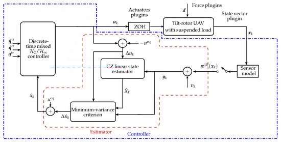
Figure 30.
Block diagram illustrating the control strategy implemented for aerial load transportation with state estimation and simulated sensors used in [22].
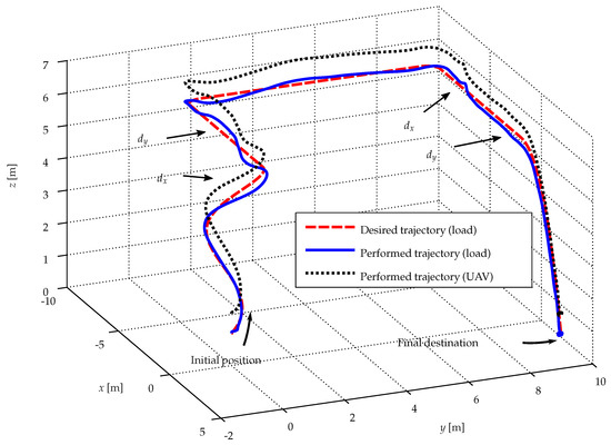
Figure 31.
Trajectory tracking in the 3D view of the ProVANT UAV 2 for load transportation, resulting from the SIL experiment. This result corresponds to the case study in Section 4.4.1.
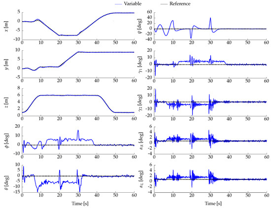
Figure 32.
Translational positions (x, y, z), attitude angles roll (), pitch (), and yaw () expressed in Euler angles using the ZYX convention about the local axes, along with the tilting angles (, ) of the right and left servomotors, and the load angles (, ), obtained from the SIL experiment. This result corresponds to the case study in Section 4.4.1.
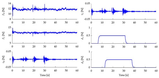
Figure 33.
Forces generated by the propellers (, ), torques applied to the thruster assemblies by the servomotors (, ), and disturbance forces acting on the load along the x and y axes of the world frame (, ), obtained from the SIL experiment. This result corresponds to the case study in Section 4.4.1.
In this case study, the ProVANT Simulator has been demonstrated to be a suitable environment for testing both control and state estimation algorithms in scenarios where onboard sensors operate at different sampling rates. It enabled the verification of correct algorithm implementation and facilitated the evaluation of the control strategy’s robustness under realistically emulated flight conditions.
4.4.2. Trajectory Tracking of the Load Using Hardware-in-the-Loop Simulation
In this case study, the ProVANT Simulator is integrated into an asynchronous HIL simulation framework to evaluate the performance and real-time feasibility of the explicit tube-based Model Predictive Control (MPC) proposed in [23].
In the control strategy, the MPC control law is precomputed offline via multi-parametric optimization, yielding a piecewise-affine policy over critical regions of the state space. At runtime, the controller identifies the region containing the current state and applies the associated affine law—avoiding online optimization and substantially reducing latency to meet real-time embedded requirements. A robust tube-based structure supplements this scheme with a secondary feedback correction derived from linear matrix inequalities (LMIs) and a robust positively invariant set for the uncertain linear parameter varying (LPV) model, compensating for model mismatch and disturbances while ensuring constraint satisfaction and robust stability.
The experimental setup consists of an NVIDIA Jetson embedded computer interfaced with the ProVANT Simulator via serial communication for the exchange of state information and control signals, as illustrated in Figure 34. The results of the HIL simulations are presented in Figure 35, Figure 36 and Figure 37. A video recording of the experiments is available at https://youtu.be/7hwKO6-Emjw. Detailed measurements of the execution time of the explicit tube-based MPC can be found in [23].
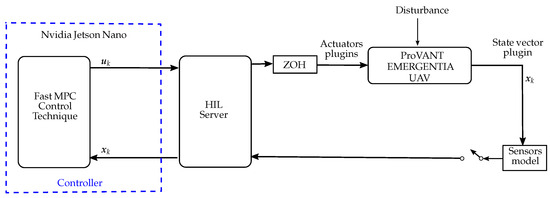
Figure 34.
Block diagram illustrating the control strategy implemented for aerial load transportation using HIL experiment.
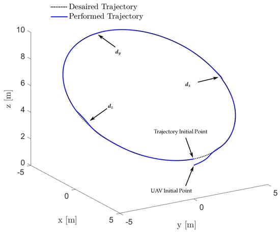
Figure 35.
Trajectory tracking in the 3D view of the ProVANT UAV 2 for load transportation, resulting from the HIL experiment. This result corresponds to the case study in Section 4.4.2.
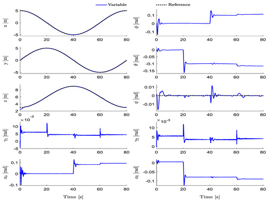
Figure 36.
Translational positions (x, y, z), attitude angles roll (), pitch (), and yaw () expressed in Euler angles using the ZYX convention about the local axes, along with the tilting angles (, ) of the right and left servomotors, and the load angles (, ). This result corresponds to the case study in Section 4.4.2.
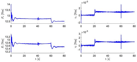
Figure 37.
Forces generated by the propellers (, ), torques applied to the thruster assemblies by the servomotors (, ). This result corresponds to the case study in Section 4.4.2.
To conclude this case study, the ProVANT Simulator enabled precise measurement of the control algorithm’s execution time on the embedded platform, as presented in Figure 38, allowing for the assessment of its compliance with real-time constraints and demonstrating that the controller is ready for deployment on the physical prototype.
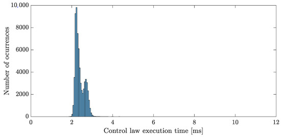
Figure 38.
Control law execution time for the case study in Section 4.4.2.
4.5. ProVANT UAV 3
This subsection presents a case study involving the ProVANT UAV 3, illustrated in Figure 39. This UAV is composed of: (i) the fuselage, where electronic components such as the battery, sensors, microprocessors, and other equipment are assembled; (ii) the thruster groups, which consist of propellers, brushless DC motors, and servomotors responsible for tilting the propellers; and (iii) the tail surfaces, comprising horizontal and vertical stabilizers, the former generating pitch moments via elevator deflection and the latter generating yaw moments via rudder deflection.
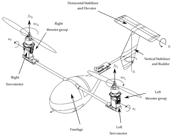
Figure 39.
The ProVANT UAV 3 mechanical design.
The ProVANT UAV 3, along with the UAVs presented in the subsequent case studies, are convertible platforms capable of transitioning between helicopter and cruise flight modes. These platforms require the integration of aerodynamic models to accurately represent their behavior. Designing control laws for such UAVs is particularly challenging due to the varying effects of relative wind across flight modes. In helicopter mode (VTOL and hovering), the low relative wind results in small aerodynamic forces. In contrast, during cruise flight, higher wind speeds enable small control surface deflections to generate significant forces and moments for effective navigation [24]. Classical linear controllers are typically inadequate to guarantee acceptable trajectory tracking performance across the full flight envelope.
The ProVANT UAV 3 features tail-surfaces that enhance the forward flight performance by improving trim stability. However, its thruster groups remain essential for both longitudinal and directional control, even in cruise flight, since the UAV lacks fixed-wing and, thereby, cannot fully transition the rotors to the horizontal position. As a result, the aircraft operates in a continuous transition/cruise mode. Its flight envelope includes vertical take-off, axial flight, hovering, transition to cruise flight at constant altitude, longitudinal plane maneuvers (movement in the x-z plane), lateral-directional plane maneuvers (movement in the x-y plane), transition from cruise to hovering, and vertical landing.
The mechanical design of the ProVANT UAV 3 was developed using SolidWorks 2024 and exported to the ProVANT simulator. The fuselage features a teardrop shape to reduce drag and enhance aerodynamic efficiency. Tail surfaces were inspired by the XV-15 aircraft, employing NACA 0009 and NACA 64A015 profiles for the vertical and horizontal stabilizers, respectively. Due to Gazebo’s lack of support for electronics and fluid dynamics simulation, the electrical dynamics of the brushless motors were assumed sufficiently fast to be neglected. Nonlinear aerodynamic coefficients for the tail surfaces were obtained from [25], while the symmetric fuselage was modeled as a symmetrical airfoil, using data from [26]. Linear interpolation was applied to all aerodynamic coefficient data to ensure smooth behavior. The simulation was through the ODE physics engine, configured with a step time of 4 ms and a controller sample time of 12 ms. Table 7 presents the parameters of the ProVANT UAV 3.
Table 7.
Parameters of the ProVANT UAV 3.
In this case study, the ProVANT Simulator is employed to conduct synchronous SIL experiment evaluating the performance of the Robust Adaptive Mixing Controller (RAMC) proposed in [27]. A comprehensive discussion of the UAV’s mathematical modeling and control design can be found in the same reference. The RAMC controller adopts a cascade structure, with the outer loop responsible for planar motion, governed by the x and y dynamics, and the inner loop handling altitude and attitude control, which includes the dynamics of z, , , , , , , , and the UAV body velocities. The outer loop kinematic controller generates desired linear velocity references, which are then tracked by the inner loop RAMC. A block diagram of the proposed control architecture is shown in Figure 40.
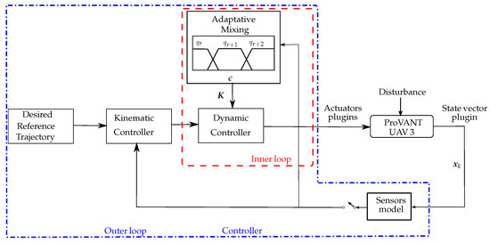
Figure 40.
Block diagram of the control strategy proposed in [27], implemented for the ProVANT UAV 3. This strategy is designed to enable operation in both helicopter and transition flight modes.
The experiment was executed on a general-purpose notebook equipped with an Intel Core i7 8750H processor (2.2 GHz), featuring six physical cores, twelve logical threads, 24 GB of RAM, and an NVIDIA GTX 1050Ti GPU, running Ubuntu Linux version 18.04. The implemented control strategy combines pre-designed linear controllers to achieve stable trajectory tracking across the entire flight envelope of the ProVANT UAV 3 while mitigating the effects of external disturbances.
The SIL experiment evaluates the UAV’s ability to follow a predefined trajectory composed of six distinct segments, as detailed in Figure 41. Accordingly, Figure 42 and Figure 43 show the time evolution of the translational position, attitude, tilt angles, applied forces and torques, and the deflections of the aerodynamic control surfaces. A video recording of the simulation is available at https://youtu.be/Lrf-QX34Wnk.
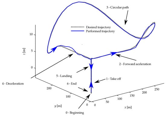
Figure 41.
Trajectory tracking in the 3D view of ProVANT UAV 3, resulting from the SIL experiment. This result corresponds to the case study in Section 4.5.
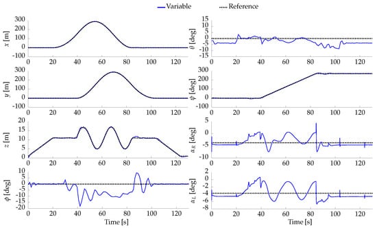
Figure 42.
Translational positions (x, y, z), attitude angles roll (), pitch (), and yaw () expressed in Euler angles using the ZYX convention about the local axes, along with the tilting angles (, ) of the right and left servomotors, obtained from the SIL experiment. This result corresponds to the case study in Section 4.5.
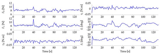
Figure 43.
Forces generated by the propellers (, ), torques applied to the thruster assemblies by the servomotors (, ), deflections of the elevator and rudder aerodynamic control surfaces (, ). This result corresponds to the case study in Section 4.5.
To conclude, the experimental results indicate that the ProVANT Simulator effectively emulated the behavior of the tilt-rotor UAV during the transition maneuver, clearly demonstrating that this operation would not be feasible without aerodynamic tail surfaces (as shown in the experiment video). Additionally, it enabled a thorough evaluation of the control strategy’s robustness under realistic flight conditions and provided evidence for the adequacy of the mathematical model employed in the controller’s design in capturing the aircraft’s dynamic behavior.
4.6. ProVANT EMERGENTIA UAV
This section presents a case study involving the ProVANT EMERGENTIA, illustrated in Figure 44. Unlike the ProVANT UAV 3, the ProVANT EMERGENTIA model features fixed wings and V-tail surfaces. During cruise flight, the wings generate significant aerodynamic lift to support sustained forward motion, allowing the rotors to be tilted horizontally and enabling the aircraft to operate in airplane mode. For further details on the proposed mathematical modeling and control law design, please refer to [28].
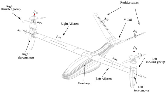
Figure 44.
The ProVANT EMERGENTIA mechanical design.
The ProVANT EMERGENTIA mechanical design was developed using Computer-Aided Three-dimensional Interactive Application (CATIA) V5 software and subsequently exported to the ProVANT Simulator. Wind tunnel experiments were conducted to determine the aerodynamic coefficients used to calculate the forces and moments generated by aerodynamic surfaces, including the propellers, fuselage, wings, tail surfaces, and aerodynamic interactions among these surfaces [29]. Table 8 presents the UAV parameters.
Table 8.
Parameters of the ProVANT EMERGENTIA UAV.
The ProVANT Simulator was employed to perform synchronous SIL experiments aiming at evaluating the effectiveness of a robust nonlinear controller addressed in [28]. This controller is a single-layer nonlinear robust optimal control strategy (see Figure 45) designed to achieve accurate trajectory tracking across the entire flight envelope of the ProVANT EMERGENTIA, while mitigating the effects of external disturbances. To conduct the experiment, Gazebo was set up with the ODE physics engine using a simulation time step of 4 ms, while the control algorithm was executed with a sample time of 12 ms. The SIL experiment was conducted on a general-purpose notebook with an Intel Core i7 8750H processor (2.2 GHz), featuring six physical cores and twelve logical threads, 24 GB of RAM, and an NVIDIA GTX 1050Ti GPU, running Ubuntu Linux version 18.04.
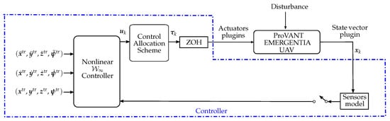
Figure 45.
Block diagram illustrating the control strategy implemented via SIL for the ProVANT EMERGENTIA UAV, designed to operate across this UAV’s entire flight envelope [28].
In the SIL experiment, the ProVANT EMERGENTIA is tasked with following a predefined trajectory composed of six distinct segments, as illustrated in Figure 46. In the first segment, the UAV must take-off from a home position while accelerating forward. In the second segment, it reaches the cruise speed (33 m/s) and performs steady forward flight at constant altitude. The third segment involves flying along a circular path while maintaining both altitude and cruise speed. Upon completing this turn, the UAV performs straight-level flight. In the fifth and sixth segments, it decelerates and performs a landing maneuver at the final destination, where it remains stationary. A video recording of the experiments is available at https://youtu.be/6P3yH5hxEaY.
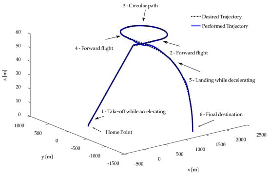
Figure 46.
ProVANT EMERGENTIA trajectory tracking in the 3D view, resulting from the SIL experiment. This result corresponds to the case study in Section 4.6.
During the experiment, external disturbances and wind gusts were applied at critical moments, specifically during the transitions from helicopter to cruise flight mode at the beginning, and from cruise back to helicopter mode at the end. As can be observed from Figure 46 and Figure 47, the control system successfully attenuated all of these disturbances. To execute the circular segment of the trajectory, the tilt-rotor UAV adopted a non-zero roll angle, a necessary physical condition to generate lateral lift and enable coordinated turning. Additionally, the system exhibited a yaw deviation due to lateral wind, reflecting realistic aerodynamic behavior. It is noteworthy that, due to the high magnitude of the relative wind speed during cruise flight, the propellers lost efficiency, requiring a higher angular velocity, as shown in Figure 48. These results confirm that the ProVANT simulator closely replicates the dynamic responses expected under real-world flight conditions.
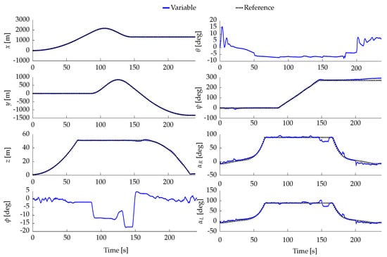
Figure 47.
Translational positions (x, y, z), attitude angles roll (), pitch (), and yaw () expressed in Euler angles using the ZYX convention about the local axes, along with the tilting angles (, ) of the right and left servomotors, obtained from the SIL experiment. This result corresponds to the case study in Section 4.6.
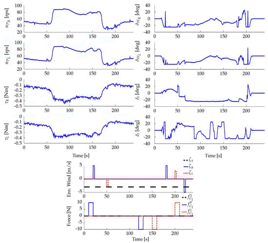
Figure 48.
Angular velocities of the propellers (, ), torques applied to the thruster assemblies by the servomotors (, ), deflections of the aerodynamic control surfaces (, ), and external disturbances (environment wind, wind gusts, and applied forces), obtained from the SIL experiment. For clarity, the tail control surfaces are represented by the equivalent elevator and rudder deflections, computed as and , where and denote the deflections of the right and left tail control surfaces, respectively. This result corresponds to the case study in Section 4.6.
4.7. VERSATILE UAV
This section presents a case study involving the VERSATILE UAV, a quadtilt-rotor aircraft depicted in Figure 49. Unlike the ProVANT EMERGENTIA, this configuration features four independently controlled propulsion groups. This capability enables the generation of greater yaw and pitch torques, which enhances the aircraft’s maneuverability at low speeds when compared to the ProVANT EMERGENTIA UAV, as discussed in [30].
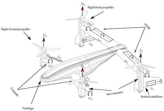
Figure 49.
The VERSATILE UAV details.
This case study aims to evaluate the stability and trajectory tracking performance of the VERSATILE UAV across its entire flight envelope under external disturbances, using a set of control strategies. To this end, five RAMC controllers, based on the same architecture, presented in Section 4.5 and illustrated in Figure 40, were implemented and tested: , , , , and . Each controller adopts a distinct design methodology to compute the mixing feedback gains used in the adaptive structure of the dynamic controller. A detailed discussion of their theoretical foundations and implementation procedures is provided in [31]. Table 9 presents the VERSATILE UAV parameters.
Table 9.
Parameters of the ProVANT VERSATILE UAV.
Asynchronous HIL experiments were conducted using the ProVANT Simulator to evaluate the controllers’ real-time performance and assess their readiness for deployment on the physical prototype. The ODE physics engine was chosen in Gazebo to experiment, taking into consideration a time step of 4 ms and a sample time of 12 ms for the controller, the latter representing the system’s real-time constraint. The control algorithm was executed in a Raspberry Pi 4 model B SBS with a quadcore ARM Cortex-A72 processor running at 1.5 GHz, with 8GB of DDR4 RAM and a VideoCore XI GPU (ARM Holdings, Cambridge, UK). The UAV was tasked with tracking the same trajectory addressed in the previous case study. The results of the HIL simulations are illustrated in Figure 50, Figure 51, Figure 52 and Figure 53, and a video of the experiments is available at https://youtu.be/GxHePSJiPKg. A histogram of the execution times for the implemented control strategies is presented in Figure 53. As shown, all strategies successfully met the real-time performance requirement.
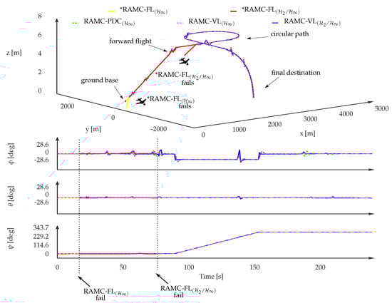
Figure 50.
Translational positions (x, y, z), attitude angles roll (), pitch (), and yaw () expressed in Euler angles using the ZYX convention about the local axes obtained from the SIL experiment. This result corresponds to the case study in Section 4.7.
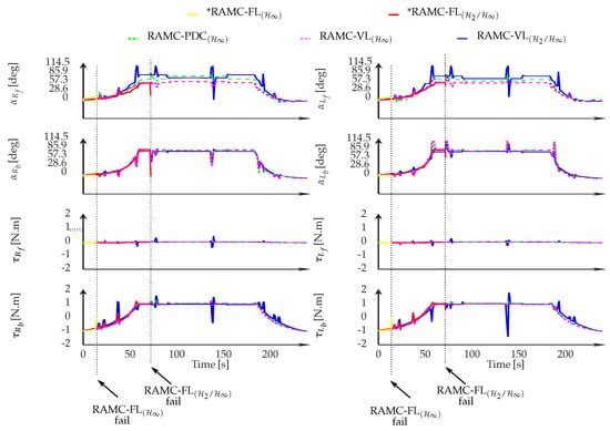
Figure 51.
Tilting angles (, , , ) of the right and left servomotors from the frontal and rear parts of the UAV, and torques applied to the thruster assemblies by the servomotors (, , , ), obtained from the HIL experiment. This result corresponds to the case study in Section 4.7.
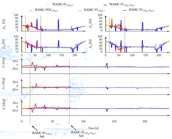
Figure 52.
Forces applied by the frontal and rear propellers (, , , ), and deflections of the aerodynamic control surfaces (, , ) obtained from the HIL experiment. This result corresponds to the case study in Section 4.7.
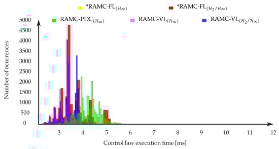
Figure 53.
Control law execution time for the case study in Section 4.7.
By offering a realistic, high-fidelity simulation environment, the ProVANT Simulator enabled rigorous testing and evaluation of various controllers, clearly exposing cases where non-robust strategies failed to maintain trajectory tracking under adverse conditions. These results highlight the simulator’s effectiveness as a valuable tool for assessing the robustness of control strategies.
5. Conclusions
The ProVANT Simulator was designed as a versatile platform to support research and development of UAV control algorithms. It provides an accurate representation of complex UAV dynamics, enabling the evaluation of control strategy performance across different scenarios. Through integration with established tools such as Gazebo and ROS, the simulator offers a modular, user-friendly environment for high-fidelity simulation-based testing, including SIL and HIL experiments.
This work presented the results of several case studies conducted using the ProVANT Simulator, featuring different UAV configurations, including quadrotors and tilt-rotors. The scenarios encompassed a range of tasks, such as aggressive maneuvers, load transportation, and transitions between helicopter and airplane flight modes. These case studies demonstrated the simulator’s ability to accurately emulate complex robotic systems and underscored its potential for validating control strategies before conducting real-world flight experiments.
Future developments will concentrate on improving the platform’s usability and extending its capabilities to include the simultaneous simulation of multi-UAV systems, along with the integration of more accurate environmental wind models. Furthermore, models for battery and drive unit power consumption are already planned and are currently under development. The UAVs featured in the case studies are currently under construction at the Federal University of Minas Gerais and the University of Seville. Data collected from upcoming real-flight experiments will be used to enhance the simulator’s fidelity. These advancements will reduce the gap between simulation and real-world UAV applications, further establishing the ProVANT simulator as a valuable resource for the aerospace, robotics, and control systems community.
Author Contributions
Conceptualization, J.E.M., D.N.C., B.S.R., R.A., I.B.P.N., J.C.P., M.A.S., L.B.B., S.E. and G.V.R.; Methodology, J.E.M., D.N.C., J.M.C., B.S.R., R.A., I.B.P.N., J.C.P., M.A.S. and G.V.R.; Software, J.E.M., D.N.C., J.M.C., B.S.R., R.A., I.B.P.N., J.C.P., D.F.S. and M.A.S.; Validation, J.E.M., D.N.C., J.M.C., B.S.R., R.A., I.B.P.N., J.C.P. and D.F.S.; Formal analysis, J.E.M., D.N.C., J.M.C., B.S.R., R.A., I.B.P.N., J.C.P., D.F.S. and M.A.S.; Investigation, J.E.M., D.N.C., J.M.C., B.S.R., R.A., I.B.P.N., J.C.P., M.A.S., S.E. and G.V.R.; Resources, J.E.M., D.N.C., B.S.R., R.A., I.B.P.N., J.C.P. and G.V.R.; Data curation, J.E.M., D.N.C., J.M.C., B.S.R., R.A., I.B.P.N., J.C.P. and G.V.R.; Writing—original draft, J.E.M., D.N.C., J.M.C., B.S.R., R.A., I.B.P.N., J.C.P., D.F.S. and G.V.R.; Writing—review and editing, J.E.M., D.N.C., B.S.R., M.A.S., L.B.B., S.E. and G.V.R.; Visualization, J.E.M., D.N.C., B.S.R., M.A.S. and G.V.R.; Supervision, D.N.C., L.B.B., S.E. and G.V.R.; Project administration, L.B.B., S.E. and G.V.R.; Funding acquisition, G.V.R. All authors have read and agreed to the published version of the manuscript.
Funding
This work was supported by the Brazilian agencies Coordenação de Aperfeiçoamento de Pessoal de Nível Superior (CAPES)—Finance Code 001—through the Academic Excellence Program (PROEX), National Council for Scientific and Technological Development (CNPq) under the grants 317058/2023-1 and 422143/2023-5, and Research Foundation of Minas Gerais (FAPEMIG) under the grant BPD-00960-22.
Data Availability Statement
The original data presented in the study are openly available in the GitHub Repository https://github.com/ProVANT-Project.
Conflicts of Interest
The authors declare no conflicts of interest.
References
- Agüero, C.E.; Koenig, N.; Chen, I.; Boyer, H.; Peters, S.; Hsu, J.; Gerkey, B.; Paepcke, S.; Rivero, J.L.; Manzo, J.; et al. Inside the virtual robotics challenge: Simulating real-time robotic disaster response. IEEE Trans. Autom. Sci. Eng. 2015, 12, 494–506. [Google Scholar] [CrossRef]
- Hambuchen, K.A.; Roman, M.C.; Sivak, A.; Herblet, A.; Koenig, N.; Newmyer, D.; Ambrose, R. Nasa’s space robotics challenge: Advancing robotics for future exploration missions. In Proceedings of the AIAA SPACE and Astronautics Forum and Exposition, Orlando, FL, USA, 12–14 September 2017; p. 5120. [Google Scholar]
- Koval, A.; Kanellakis, C.; Vidmark, E.; Haluska, J.; Nikolakopoulos, G. A subterranean virtual cave world for gazebo based on the DARPA SubT challenge. arXiv 2020, arXiv:2004.08452. [Google Scholar] [CrossRef]
- Pizetta, I.H.B.; Brandão, A.S.; Sarcinelli-Filho, M. A Hardware-in-the-Loop Platform for Rotary-Wing Unmanned Aerial Vehicles. J. Intell. Robot. Syst. 2016, 84, 725–743. [Google Scholar] [CrossRef]
- Furrer, F.; Burri, M.; Achtelik, M.; Siegwart, R. RotorS—A Modular Gazebo MAV Simulator Framework; Springer: Berlin/Heidelberg, Germany, 2016; Volume 625, pp. 595–625. [Google Scholar] [CrossRef]
- Koubâa, A.; Allouch, A.; Alajlan, M.; Javed, Y.; Belghith, A.; Khalgui, M. Micro Air Vehicle Link (MAVlink) in a Nutshell: A Survey. IEEE Access 2019, 7, 87658–87680. [Google Scholar] [CrossRef]
- Chitta, S.; Marder-Eppstein, E.; Meeussen, W.; Pradeep, V.; Tsouroukdissian, A.R.; Bohren, J.; Coleman, D.; Magyar, B.; Raiola, G.; Lüdtke, M.; et al. ros_control: A generic and simple control framework for ROS. J. Open Source Softw. 2017, 2, 456. [Google Scholar] [CrossRef]
- Dimmig, C.A.; Silano, G.; McGuire, K.; Gabellieri, C.; Hönig, W.; Moore, J.; Kobilarov, M. Survey of Simulators for Aerial Robots: An Overview and In-Depth Systematic Comparisons. IEEE Robot. Autom. Mag. 2024, 32, 2–15. [Google Scholar] [CrossRef]
- Hentati, A.I.; Krichen, L.; Fourati, M.; Fourati, L.C. Simulation Tools, Environments and Frameworks for UAV Systems Performance Analysis. In Proceedings of the 14th International Wireless Communications & Mobile Computing Conference, Limassol, Cyprus, 25–29 June 2018; pp. 1495–1500. [Google Scholar] [CrossRef]
- Xie, D.; Hu, R.; Wang, C.; Zhu, C.; Xu, H.; Li, Q. A Simulation Framework of Unmanned Aerial Vehicles Route Planning Design and Validation for Landslide Monitoring. Remote Sens. 2023, 15, 5758. [Google Scholar] [CrossRef]
- Gill, J.S.; Saeedi Velashani, M.; Wolf, J.; Kenney, J.; Manesh, M.R.; Kaabouch, N. Simulation Testbeds and Frameworks for UAV Performance Evaluation. In Proceedings of the IEEE International Conference on Electro Information Technology, Mount Pleasant, MI, USA, 14–15 May 2021; pp. 335–341. [Google Scholar] [CrossRef]
- Koenig, N.; Howard, A. Design and use paradigms for gazebo, an open-source multi-robot simulator. In Proceedings of the 2004 IEEE/RSJ International Conference on Intelligent Robots and Systems (IROS) (IEEE Cat. No.04CH37566), Sendai, Japan, 28 September–2 October 2004; Volume 3, pp. 2149–2154. [Google Scholar]
- Koubaa, A. Robot Operating System (ROS): The Complete Reference (Volume 2), 1st ed.; Springer: Berlin/Heidelberg, Germany, 2017. [Google Scholar]
- Nascimento, I.B.P. Nonlinear Model Predictive Control Strategies for Autonomous Vehicles in Unknown Environments. Master’s Thesis, Federal University of Minas Gerais, Belo Horizonte, Brazil, 2020. [Google Scholar]
- Raffo, G.V. Robust Control Strategies for a Quadrotor Helicopter: An Underactuated Mechanical System. Ph.D. Thesis, Universid de Sevilha, Seville, Spain, 2011. [Google Scholar]
- Andersson, J.A.; Gillis, J.; Horn, G.; Rawlings, J.B.; Diehl, M. CasADi: A Software Framework for Nonlinear Optimization and Optimal Control. Math. Program. Comput. 2019, 11, 1–36. [Google Scholar] [CrossRef]
- Pereira, J.C.; Leite, V.J.S.; Raffo, G.V. Stabilizing NMPC Approaches for Underactuated Mechanical Systems on the SE(3) Manifold. arXiv 2025, arXiv:2503.17458. [Google Scholar] [CrossRef]
- de Morais, J.E.; Cardoso, D.N.; Raffo, G.V. Robust Nonlinear Control of Aerial Manipulators. J. Control. Autom. Electr. Syst. 2023, 34, 1–17. [Google Scholar] [CrossRef]
- Suarez, A.; Vega, V.M.; Fernandez, M.; Heredia, G.; Ollero, A. Benchmarks for Aerial Manipulation. IEEE Robot. Autom. Lett. 2020, 5, 2650–2657. [Google Scholar] [CrossRef]
- Choset, H.; Lynch, K.; Hutchinson, S.; Kantor, G.; Burgard, W.; Kavraki, L.; Thrun, S. Principles of Robot Motion: Theory, Algorithms, and Implementations; MIT Press: Cambridge, UK, 2005; p. 603. [Google Scholar]
- Coleman, D.; Sucan, I.; Chitta, S.; Correll, N. Reducing the Barrier to Entry of Complex Robotic Software: A MoveIt! Case Study. J. Softw. Eng. Robot. 2014, 1, 1–14. [Google Scholar]
- Rego, B.S.; Raimondo, D.M.; Raffo, G.V. Path Tracking Control with State Estimation based on Constrained Zonotopes for Aerial Load Transportation. In Proceedings of the 57th IEEE Conference on Decision and Control, Miami, FL, USA, 17–19 December 2018; pp. 1979–1984. [Google Scholar]
- Andrade, R.; Ferramosca, A.; Normey-Rico, J.E.; Raffo, G.V. Tube-Based Explicit Model Predictive Control for a Tiltrotor UAV in Cargo Transportation Tasks. J. Control. Autom. Electr. Syst. 2024, 35, 1039–1058. [Google Scholar] [CrossRef]
- Morin, P. Modeling and control of convertible Micro Air Vehicles. In Proceedings of the Robot Motion and Control (RoMoCo), 2015 10th International Workshop on IEEE, Poznan, Poland, 6–8 July 2015; pp. 188–198. [Google Scholar]
- Ferguson, S.W. A Mathematical Model for Real Time Flight Simulation of a Generic Tilt-Rotor Aircraft. NASA CR-166536. 1988. Available online: https://rotorcraft.arc.nasa.gov/Publications/files/CR-166536_882.pdf (accessed on 30 June 2025).
- Sheldahl, R.E.; Klimas, P.C. Aerodynamic Characteristics of Seven Symmetrical Airfoil Sections Through 180-Degree Angle of Attack for Use in Aerodynamic Analysis of Vertical Axis Wind Turbines; Technical Report; Sandia National Labs.: Albuquerque, NM, USA, 1981. [Google Scholar]
- Cardoso, D.N.; Esteban, S.; Raffo, G.V. A new robust adaptive mixing control for trajectory tracking with improved forward flight of a tilt-rotor UAV. ISA Trans. 2021, 110, 86–104. [Google Scholar] [CrossRef] [PubMed]
- Cardoso, D.N. Robust Control Framework in the Weighted Sobolev Space. Ph.D. Thesis, Universidade Federal de Minas Gerais, Belo Horizonte, Brazil, 2021. [Google Scholar]
- Ortega, F.J.; Nunez, M.; Esteban, S. Aerodynamics and Propulsive Modeling of a Bi-Rotor Convertible Aircraft for the Identification of Trim Conditions in Longitudinal Flight. In Proceedings of the Vertical Flight Society’s 77th Annual Forum & Technology Display (VFS2021), Virtual, 10–14 May 2021; pp. 1–15. [Google Scholar]
- Allenspach, M.; Ducard, G.J.J. Nonlinear model predictive control and guidance for a propeller-tilting hybrid unmanned air vehicle. Automatica 2021, 132, 109790. [Google Scholar] [CrossRef]
- Campos, J.M.; Cardoso, D.N.; Esteban, S.; Raffo, G.V. Enhanced robust adaptive flight control for a convertible VTOL UAV. J. Frankl. Inst. 2024, 361, 106663. [Google Scholar] [CrossRef]


Disclaimer/Publisher’s Note: The statements, opinions and data contained in all publications are solely those of the individual author(s) and contributor(s) and not of MDPI and/or the editor(s). MDPI and/or the editor(s) disclaim responsibility for any injury to people or property resulting from any ideas, methods, instructions or products referred to in the content. |
© 2025 by the authors. Licensee MDPI, Basel, Switzerland. This article is an open access article distributed under the terms and conditions of the Creative Commons Attribution (CC BY) license (https://creativecommons.org/licenses/by/4.0/).