Abstract
In this study, we analyzed the imaging maneuver time, retargeting maneuver time, and attitude maneuvering characteristics in the imaging section (Phase 1) and retargeting maneuver section (Phase 2) when taking multiple-target images in squint spotlight mode in a single pass of a passive SAR satellite. In particular, the synthetic aperture time and attitude maneuvering characteristics in the staring and sliding spotlight modes that can image the wider swath width while maintaining high resolution were compared and analyzed. In the sliding spotlight mode, the rotation center was located below the ground surface when the satellite was maneuvering towards the target. Steering and sliding maneuvers were performed when targeting, and the synthetic aperture time of the sliding spotlight was longer than that of the staring spotlight because overlapping imaging was performed on the point target. The satellite maneuvering during imaging can be considered as a time-fixed problem, because it was performed within synthetic aperture time according to resolution, incidence angle, swath width, etc., by minimizing the Doppler centroid variation. In order to optimize the retargeting maneuver time, an optimal analysis of the attitude maneuvering was carried out and the validity of the optimal analysis algorithm was confirmed. Finally, the scenario was analyzed by assuming a problem of imaging four targets with 5 × 5 km swath width in a 20 km × 20 km densely populated area. It was confirmed that if a squint angle of ±12 degrees is provided in a single pass, four high resolution images of 5 km × 5 km can be imaged in the sliding spotlight mode.
1. Introduction
Due to the recent miniaturization/light weight of satellites, the passive SAR satellite that requires mechanical beam steering is in the limelight, implementing a foldable reflector antenna with high storage efficiency instead of an active SAR satellite that performs electronic beam steering using a phased array antenna. Hybrid SAR satellites having the function of electronic beam steering, as well as mechanical beam steering, according to the required mission operation modes, have also been developed and/or are in operation. TecSAR [1] developed by IAI in Israel and Compact SAR [2] by TASI in Italy are the representative examples. SAR-Lupe [3] of OHB in Germany and ASNARO-2 [4] of Mitsubishi in Japan are representative passive SAR satellites.
Meanwhile, along with the development of ultra-lightweight mesh reflector antenna technology, the development and operation of new ultra-small SAR satellites are also on the rise. In addition to Capella’s Sequoia satellite [5], which successfully launched and started operation at the end of August 2020, Japanese startup company iQPS developed and successfully launched a 100 kg-class ultra-small SAR satellite at the end of 2019, but the initial operation of the satellite failed, and a subsequent satellite is currently being prepared for launch [6].
Compared to active SAR satellites using electronic beam steering, passive SAR satellites with mechanical beam steering perform imaging through attitude maneuvering of the satellite, not beam maneuvering. Therefore, in the case of active SAR satellites, since beam steering is required for spotlight mode imaging, high agility is not necessary for the satellite. However, in the case of passive SAR satellites, a highly agile satellite is required to enhance the imaging capability because the satellite itself must maneuver. Therefore, it is necessary to optimize target pointing and retargeting maneuvers to be able to image targets for a short period of time. In the case of passive SAR satellites, since beam steering is performed by satellite attitude control, the ability to take broadside mode images is limited, so squint mode operation is performed to enhance the imaging capability in spotlight mode. Unlike the broadside mode, which takes images from a position perpendicular to the target, the squint mode can increase the number of images because the antenna is pointed forward or backward from the perpendicular position by a squint angle [7].
Operation in squint mode of a large angle requires pitch and yaw, as well as roll maneuvers. There have been few published studies on squint attitude maneuvering in the spotlight mode of passive SAR satellite requiring mechanical beam steering. The squint maneuvering is very effective at taking more images in a single pass. Most of the research on the squint spotlight mode has focused on SAR processing and algorithm development related to image quality [8,9,10].
In order to take as many images as possible when a satellite passes an Area of Interest (AoI), it is required to optimize the synthetic aperture time, the retargeting maneuver time, and attitude maneuvering for both. For passive SAR satellites with mechanical beam steering, this means that the satellite’s agility capability is critical. That is, to analyze the imaging capability of continuous targets in a single pass of the satellite, analysis of the imaging maneuver time, retargeting maneuver time, and attitude maneuvering for both phases is required. In this paper, we analyze the synthetic aperture time, retargeting maneuver time, and maneuver characteristics in the imaging, as well as the retargeting maneuver stages in the staring and sliding spotlight imaging modes of passive SAR satellites.
2. Analysis of Attitude Maneuvering and Maneuver Time of Squint SAR Satellite Spotlight Mode
2.1. Attitude Maneuvering Problem in Squint Spotlight Mode
When imaging continuous targets in the spotlight mode of a passive SAR satellite, it can be divided into three different maneuvering stages. These include the imaging maneuver for synthetic aperture, the retargeting maneuver for continuous target imaging, and the operational maneuver for transmitting the taken image to the ground station. After the images are transmitted, the satellite is returned to the basic attitude (sun pointing or default incidence angle), which is also classified in the operational maneuver.
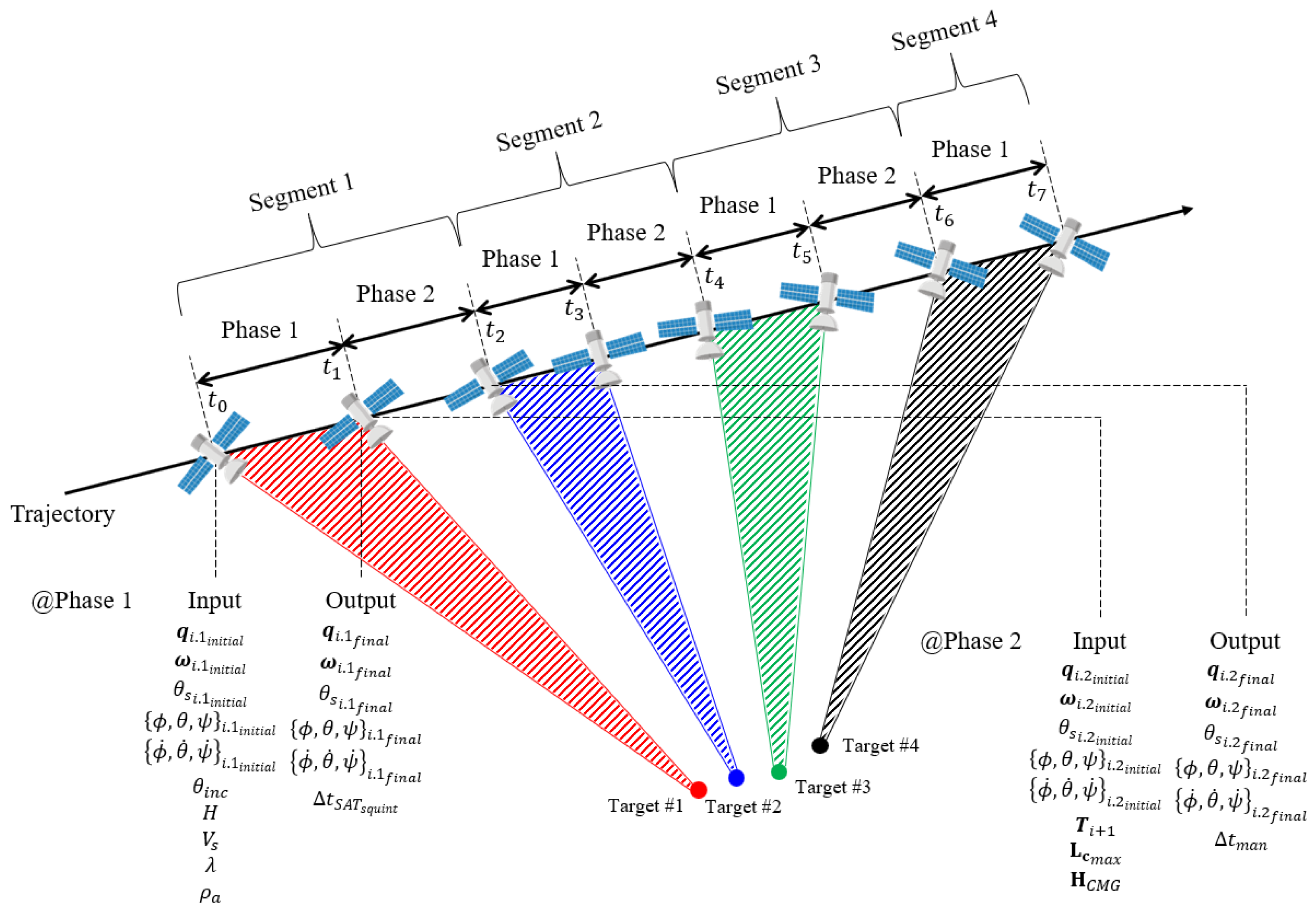
In this study, as shown in Figure 1, we analyze the optimal control characteristics of the imaging maneuver (Phase 1) and the retargeting maneuver (Phase 2) required for continuous imaging. Phase 1 is a stage in which an image of a target is taken while minimizing the Doppler centroid variation, and an attitude maneuver for imaging is performed at the same time. Phase 2 refers to the section in which a retargeting maneuver is performed to image the next target and includes stabilization time.

Figure 1.
Attitude maneuvering problem in squint spotlight mode of passive SAR satellite.
When imaging in broadside spotlight mode, it is necessary to perform yaw and pitch attitude maneuvering to minimize the Doppler centroid variation caused by the Earth’s rotation and elliptical orbit characteristics. When imaging in the squint spotlight mode, the imaging maneuver and synthetic aperture time, and the retargeting maneuver and its optimal maneuver time, are calculated by considering the three-dimensional attitude maneuvering for the yaw and pitch axes, as well as the roll axis. For each segment, Phase 2 starts immediately after Phase 1 ends, and after Phase 2 ends, Phase 1 of the next segment begins. Accordingly, in each segment and Phase, the conditions as in Equation (1) must be satisfied, and the total time until the last target is imaging is calculated.
For such an imaging maneuver for Phase 1, both the attitude to start accurate target imaging and the attitude rotation for targeting must be satisfied. In addition, squint maneuvering should be performed while minimizing the Doppler centroid variation to acquire SAR images during target pointing. It can be defined as the problem of time-fixed maneuvering during Phase 1. In order to maneuver a satellite during Phase 2, the command of the satellite must be generated in the form of feedforward control based on the attitude maneuvering profile. In addition, in order to generate the corresponding guidance profile, it is necessary to consider the maneuvering to the required target with a minimum time and a torque limit that can be generated by the actuator. It can be defined as the problem of time-min maneuvering during Phase 2.
In the past, many studies have been conducted [11,12] in which the satellite maneuvering was converted to the problem of eigen-axis rotation instead of 3-axis rotation. The eigen-axis rotation problem has the advantage of being able to simply derive a guidance profile. However, in the case of the eigen-axis rotation problem, the rotation axis is determined by the initial line-of-sight vector and the line-of-sight vector at the end of maneuvering, and it is suitable for rest-to-rest maneuvering because it assumes that there is no rate at the start and end of maneuvering. In the problem of imaging the next target after previous spotlight mode imaging of a passive SAR satellite, the retargeted maneuvering is required toward the next target and it can be defined as a spin-to-spin problem. In the case of spin-to-spin maneuvering, there are some limitations in optimizing the retargeting maneuver in the spotlight mode of a passive SAR satellite by applying the eigen-axis rotation problem.
In this study, it was defined as a problem of deriving a guidance profile to minimize the retargeting maneuver time in the spotlight mode of a passive SAR satellite that requires satellite attitude maneuvering. The retargeting maneuver problem was defined as the two points boundary value problem (TPBVP), and the maneuvering profile was derived using GPOPS-II, which is an optimal control software [13].
2.2. Timeline Elements of Mission Operation in Spotlight Mode
The mission operation in spotlight mode of SAR satellites consists of the following time elements. The spotlight mode operation in SAR satellite repeats the synthetic aperture Time () for illuminating a target at a constant speed during imaging, retargeting maneuver time (RMT; ) for pointing the next target after imaging the previous image, and stabilization time for taking subsequent images. Of course, the transmission time of the command during a single pass of the satellite to the satellite, the telemetry transmission time of the image data to the ground, and the satellite health data are also included. To increase the number of images in a single pass, it is necessary to minimize the synthetic aperture time during imaging, RMT, and stabilization time.
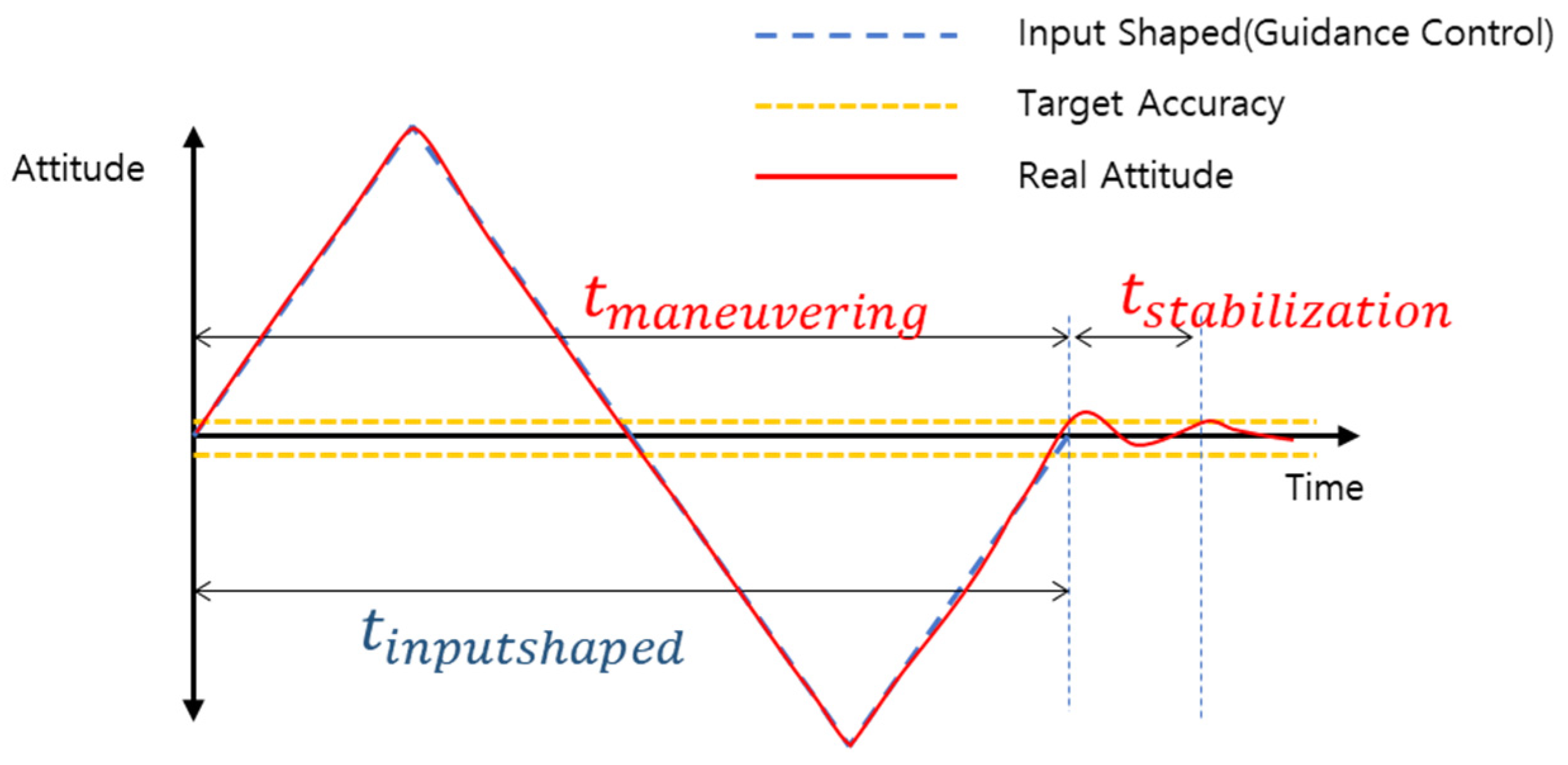
The modal frequency and mode gain of the flexible structure were assumed to consider the stabilization time. Based on the pointing accuracy and pointing stability, the appropriate jerk is analytically selected so that there is no need for stabilization time due to the flexible structure. In other words, a suitable jerk is selected to be from the mechanical aspect. Each time element for stabilization, maneuvering, and input-shaped is defined as shown in Figure 2.
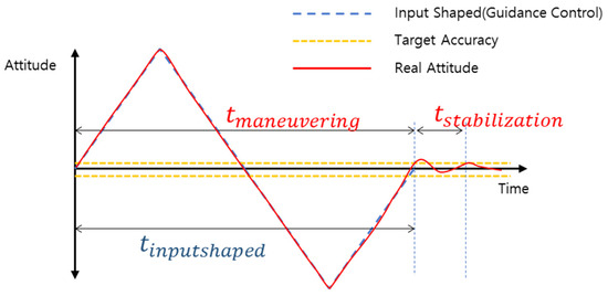
Figure 2.
The depiction of maneuvering time, stabilization time, and input shaped time.
However, the stabilization time of the satellite is allocated in consideration of error factors such as the control loop error of the attitude control system and the imbalance of the actuator, which is required to guarantee the image quality. In this study, a stabilization time of 2 s is arbitrarily assumed in consideration of these unpredictable factors.
2.3. Synthetic Aperture Time and Attitude Maneuvering during Imaging (Phase 1)
When operating the squint spotlight mode in Phase 1, the synthetic aperture time (SAT) can be calculated by considering the required resolution, squint angle, incidence angle, and swath width. During the imaging time, the attitude maneuvering profile of the satellite should be derived so that the Doppler centroid variation is minimized according to the current location of the satellite and the location of the target.
2.3.1. Synthetic Aperture Time in Broadside and Squint Staring Spotlight Modes
Figure 3 shows illuminated geometry at the broadside staring spotlight mode. In Figure 3, and are the incidence angle and slant range at the aperture center, respectively. is the look angle, and are the synthetic aperture angle (SAA) and the synthetic aperture length (SAL), respectively. is the velocity of the satellite, is the radius of the Earth, point is the center of (the) Earth. As shown in Figure 3, when assuming the Earth is flat, and become the same.
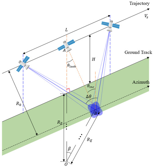
Figure 3.
Illuminated geometry of broadside staring spotlight mode.
However, considering the curvature of the Earth, when is large, the difference from becomes large. Considering the curvature of the Earth, at the aperture center can be obtained using the trigonometric formula. Using the sine law in , it can be expressed as Equation (2).
Since , must be obtained first to obtain , and can be obtained from Equation (3).
From obtained through Equation (3), can be obtained, and then in Equation (2) can be obtained.
Imaging of the SAR satellite is achieved using the Doppler shift. Therefore, the azimuth resolution can be obtained using the Doppler bandwidth , and the equation can be expressed as Equation (4) [14].
The synthetic aperture angle can be obtained using the azimuth resolution obtained in Equation (4) and expressed as Equation (5).
In Equation (5), is the wavelength of the X-band. The synthetic aperture length in spaceborne SAR can be calculated using the SAA obtained in Equation (5). If the curvature is considered, SAL becomes an arc shape, and the equation for obtaining the length of the arc is as shown in Equation (6).
Therefore, the SAT in broadside staring spotlight mode can be calculated as Equation (7).
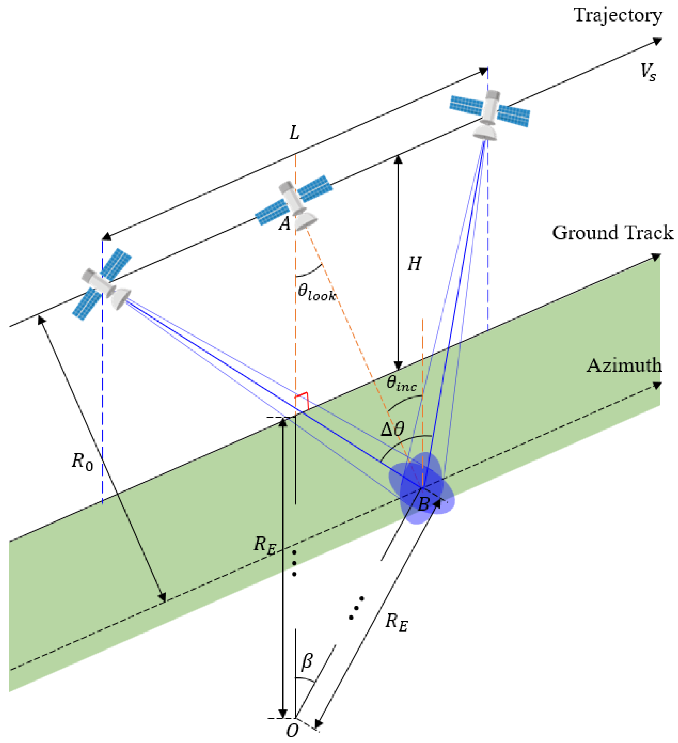
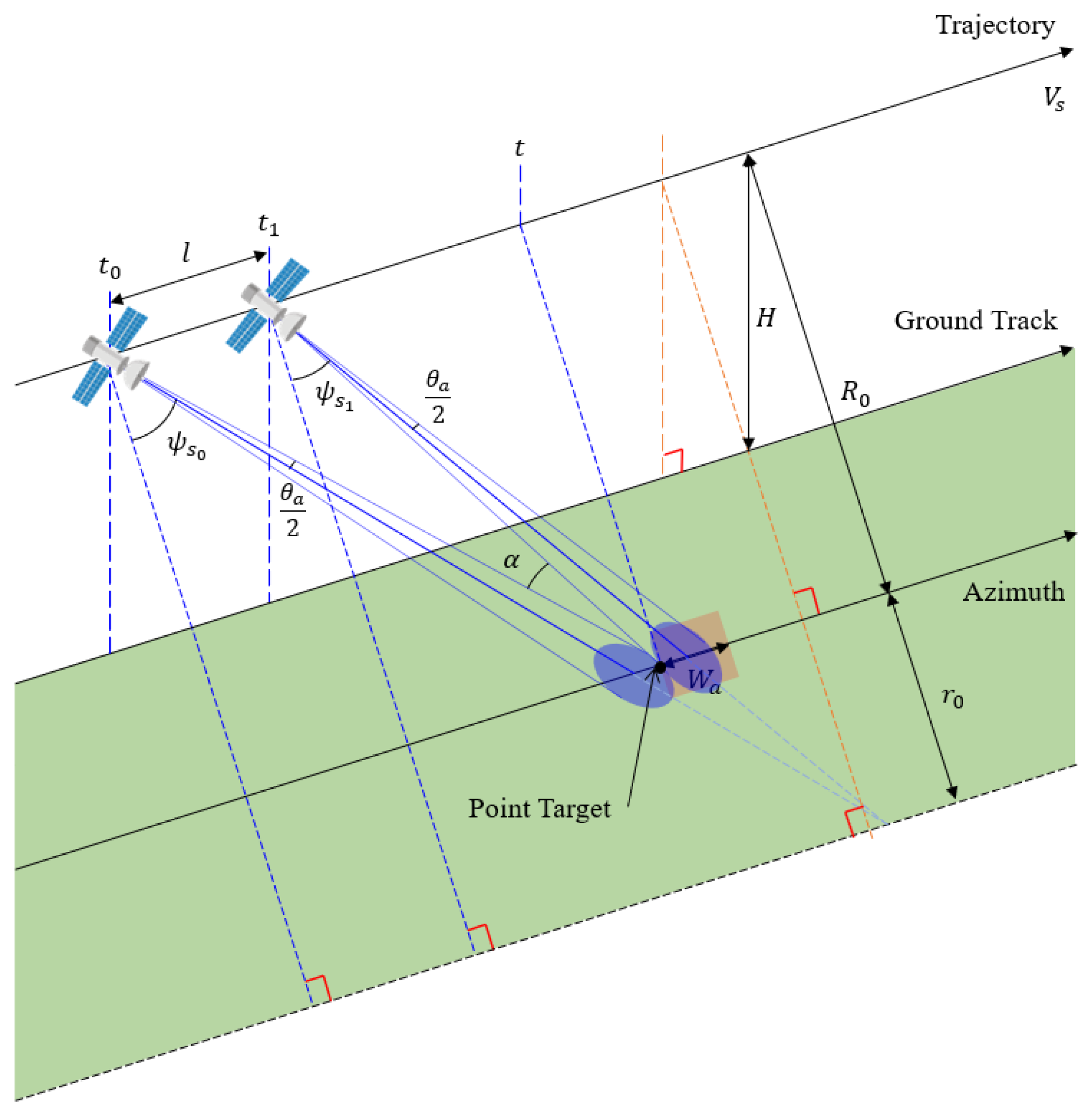
Figure 4 shows the geometry when imaging through squint maneuvering in the staring spotlight mode.
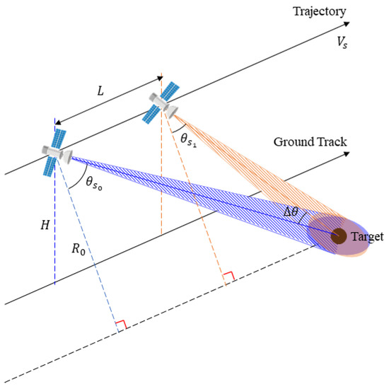
Figure 4.
Illuminated geometry of the squint staring spotlight mode.
In Figure 4, SAA can be expressed as Equation (8) because it can also be expressed as the difference between the squint angle at the start of imaging and the squint angle at the end of imaging.
Therefore, if the squint angle at the start of imaging is known, the squint angle at the end can be obtained from Equation (8).
When imaging continuous targets, the first target can set the maximum squint angle at the start of imaging that can be provided in the satellite design, and can be calculated from Equation (8). Since the squint angle is the angle between the satellite and the target when the retargeting maneuver ends in Phase 2 of the previous segment from imaging of the second target, the squint angle at the start of imaging is calculated from Equation (9). The squint angle at the ended imaging can be obtained by substituting this angle into Equation (8).
In Equation (9), is the vector of the satellite pointing to the target and is the velocity vector of the satellite in the ECEF coordinate system (see Figure 9). The derivation of Equation (9) is covered in detail in Section 2.3.3. Finally, SAL can be obtained using Equation (8) and can be expressed as Equation (10).
SAT in squint staring spotlight mode can be obtained by dividing SAL by the velocity of the satellite, as shown in Equation (11).
Imaging is performed through pitch maneuvers, but due to the influence of the Earth’s rotation, roll and yaw maneuvers must also be considered. In this analysis, a margin of 25% is considered in addition to the staring spotlight mode SAT obtained from Equations (7) or (11).
2.3.2. Synthetic Aperture Time in Broadside and Squint Sliding Spotlight Mode
In the sliding spotlight mode, unlike the staring spotlight, in which the beam center of the satellite is pointed to the target on the ground surface, the sliding spotlight mode is pointed to a point (center of rotation) below the ground surface. In sliding spotlight mode, the point target on the ground surface is overlappingly imaged, so it can be regarded as a combination of sub-apertures, and imaging is continuously performed through steering and sliding. Therefore, the sliding spotlight mode can image a wider area while maintaining the same resolution than the staring spotlight mode. For the sliding spotlight mode analysis, the following assumptions are made [15]. First, it is assumed that the maximum scene length in the direction of the azimuth and the range is set to 5 km and that the scene area is flat. Considering that the scene area is flat and there is a curvature, the height difference between the coordinates of the point target in the corner of the scene is up to 4 m [16]. Therefore, when analyzing the slant range for a point target within a scene edge in an assumed situation, it can be calculated through a simple formula without a large error. Second, it is assumed that the swath width in the range direction of the antenna beam reaching the ground surface is longer than the distance in the range direction of the scene. Third, the velocity of the satellite () is the relative velocity with respect to the scene, and the squint angle is the angle between the cross-track vector and the target vector when the center of the beam is directed toward the center of rotation. Based on this assumption, the geometry of the broadside sliding spotlight mode is shown in Figure 4. The rotation center is required to calculate the spotlight scene parameters and the azimuth steering profile of the antenna, as well as the SAT in sliding spotlight mode.
The notations presented in Figure 5 are the same as those presented in Figure 3. Additionally, is the antenna beamwidth and is the swath width. Considering the curvature of the Earth, can be obtained through Equations (2) and (3) in the same way as when calculating the slant range in staring spotlight mode.
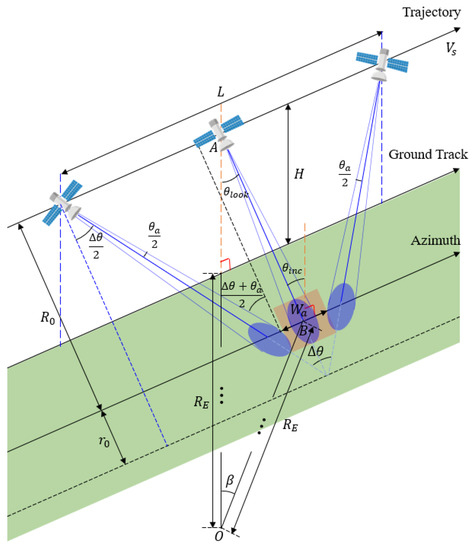
Figure 5.
Illuminated geometry of broadside sliding spotlight SAR.
As described above, in the sliding spotlight mode, the imaging center is located below the surface and the area above the surface is imaged. Figure 6 shows the geometry of the SAR satellite in broadside sliding spotlight mode for the point targets in the target scene to be imaged.

Figure 6.
Image-taking geometry of a point target within target scene for broadside sliding spotlight SAR.
Since and , Equation (12) can be expressed simply as Equation (13).
Since the squint angle in the broadside collection mode is a small angle, it can be approximated by and . Therefore, Equation (13) can be expressed as Equation (14), which is the same as the angular difference between the beams at the start and end of imaging for point targets.
Considering the curvature of the Earth, the distance that the SAR satellite moved while imaging point targets at high resolution in Figure 6 can be approximated by the length of an arc with the radius and angle , as shown in Equation (15), and it can be calculated based on the point targets and the squint angle at the start and end of imaging, respectively.
In Equation (15), all of , , and are known or can be obtained through calculations, so can be computed as in Equation (16).
In Figure 5, the SAL can be calculated from the center of imaging below the surface and the midpoint of the imaging area above the surface, respectively, and can be expressed as Equation (17).
In broadside mode, it can be approximated by and . If Equation (17) is summarized for SAA, it can be expressed as Equation (18).
By substituting Equation (18) into Equation (17) to obtain SAL and then dividing it by the velocity of the satellite, the SAT in broadside sliding spotlight mode can be obtained as Equation (19).
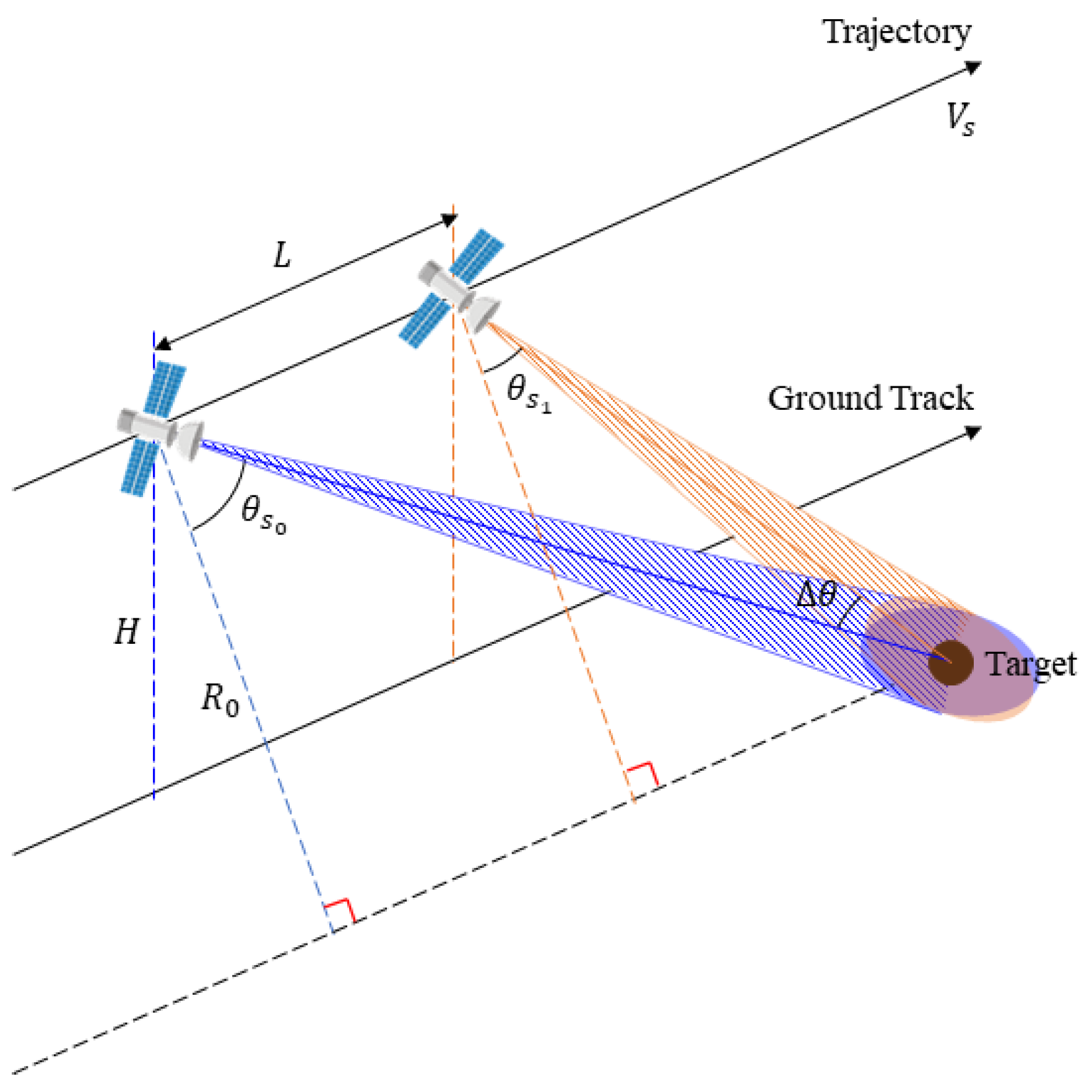
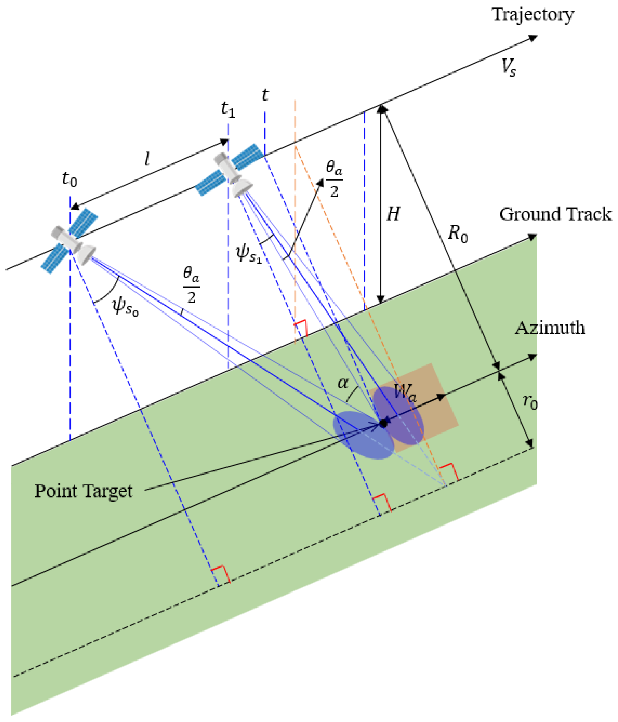
The geometry when imaging in squint sliding spotlight mode is shown in Figure 7.
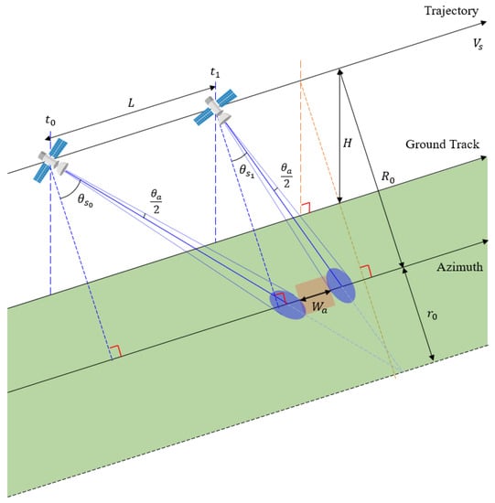
Figure 7.
Illuminated geometry of squint sliding spotlight mode SAR.
The notations presented in Figure 7 are the same as those presented in Figure 4. Additionally, is the antenna beamwidth and is the swath width. Considering the Earth’s curvature, can be obtained through Equations (2) and (3) in the same way as the method obtained in broadside sliding spotlight mode.
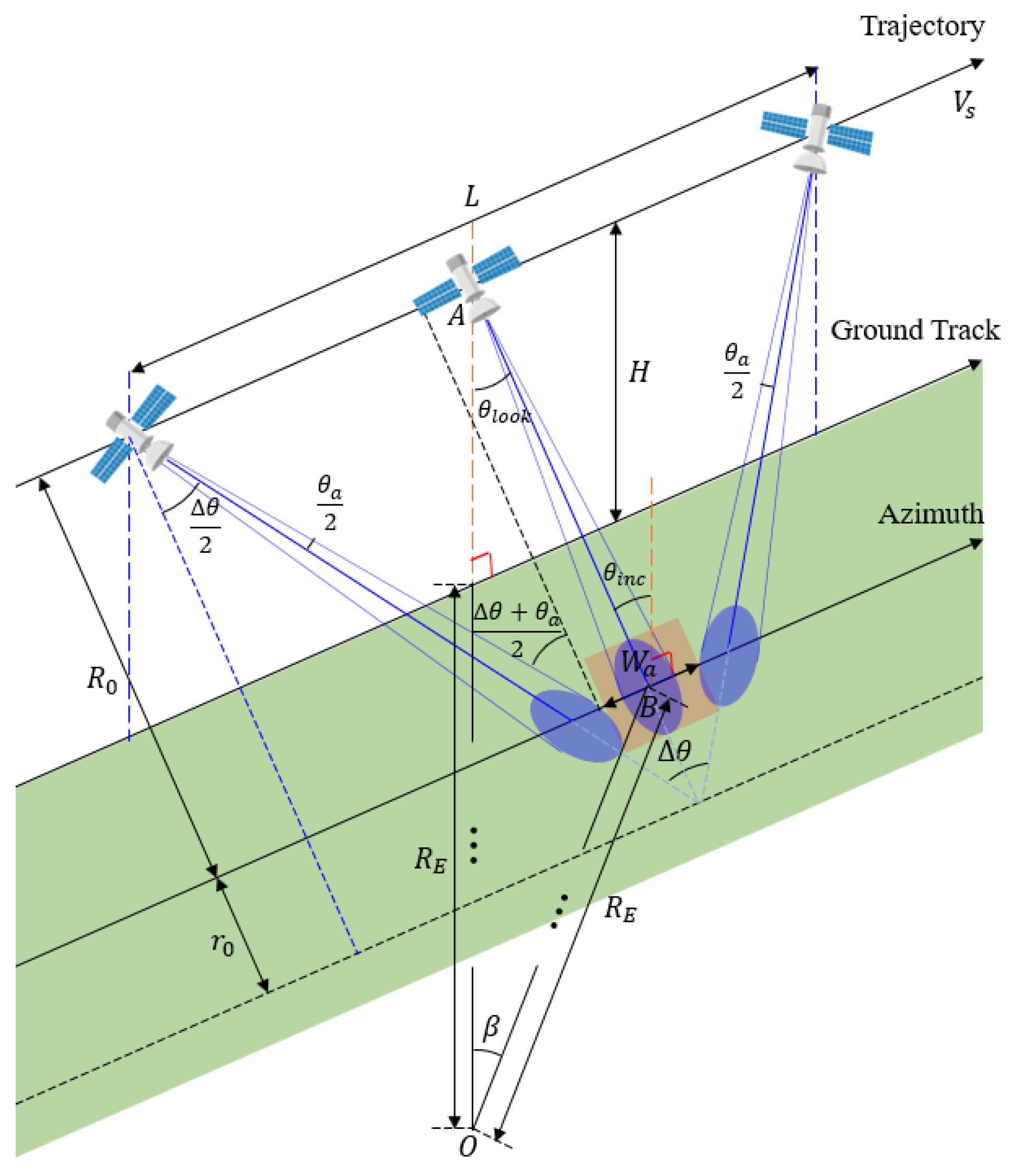
Figure 8 illustrates the imaging geometry of the SAR satellite in squint sliding spotlight mode for point targets in the area to be imaged.
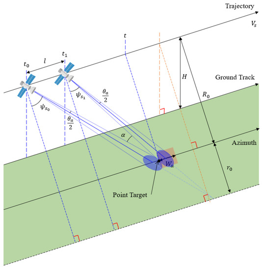
Figure 8.
Image-taking geometry of a point target within target scene for the squint sliding spotlight mode.
In Figure 8, is the squint angle at the start time of imaging for the point targets and is the squint angle at end time of imaging for the point targets. These squint angles are within the range of squint angles at the start and end of imaging in the squint mode in Figure 7. is the distance that the satellite has moved during the point targets imaging.
The azimuth resolution for point targets can be obtained through Equation (12) in the same way as in the broadside collection mode and can be simply expressed as Equation (13). However, since the squint angle is larger than that of the broadside collection mode, and cannot be approximated. Therefore, to obtain in Figure 8, the squint angle should be computed at the end of imaging, as shown in Equation (20) using Equation (13).
Using Equation (20), in Figure 8 can be expressed as Equation (21).
Since all of , , and are known or can be obtained through calculation, can be found through Equations (15) and (16) in the same way as in the broadside collection mode. In Figure 8, SAL can be calculated and expressed as Equation (22) using the point where the beam and the target meet at the start and end of imaging or the imaging center below the ground surface.
To calculate SAL in Equation (22), we first need to find . If Equation (22) is expressed as an equation for , it can be expressed as a quadratic equation for , as shown in Equation (23).
can be obtained using the quadratic formula of Equation (23), and the squint angle at the end of imaging can be found. At this time, one of the two solutions included in the required squint angle range is selected.
Using and previously obtained values, the SAL of Equation (22) can be computed, and by dividing this by the velocity of the satellite, the SAT in the squint sliding spotlight mode can be calculated, as shown in Equation (24).
As described above, image-taking is performed through pitch maneuvers, but due to the influence of the Earth’s rotation, roll and yaw maneuvers must also be considered. In this analysis, a margin of 25% is considered in addition to SAT at the sliding spotlight mode obtained from Equations (19) or (24).
2.3.3. Attitude Maneuvering for Imaging in Squint Staring and Squint Sliding Spotlight Modes
In this analysis, it is assumed that when the satellite enters the communication area, it maneuvers to point at the first target through the squint maneuver. During imaging (Phase 1), through the position, velocity, and initial angular velocity of the satellite in the ECEF coordinate system and the attitude of the satellite that minimizes the Doppler centroid variation, it can be expressed kinematically using quaternion. In addition, the angular velocity of the satellite can be obtained from the equation of the quaternion’s kinematics [17]. The angular velocity of the satellite is that for the three principal axes of the satellite body frame. The quaternion and the angular velocity of the satellite at the end of imaging are used as input data for optimization in the next Phase 2 retargeting maneuver section.
To perform transformation using the concept of quaternion, the attitude transformation matrix from the LVLH (Local Vertical Local Horizontal) coordinate system to the satellite body frame can be expressed using the DCM (Direction Cosine Matrix) [17]. Even if the quaternion is known, it is difficult to intuitively determine the attitude of the satellite, so we can recognize it more easily by converting to a Euler angle. In addition, the Euler rate can be obtained by using the Euler angle and the angular velocity of the satellite obtained through the kinematic equation of the previous quaternion [18].
In the case of squint imaging of passive SAR satellites, a satellite attitude maneuvering strategy should be derived to minimize Doppler centroid variation. For this, we consider an attitude maneuvering method based on the iso-Doppler surface where the same Doppler centroid variation occurs [19]. The iso-Doppler surface in the squint staring spotlight mode is in the form of a conic shape, as shown in Figure 9, where is the axis of rotation of the cone (the vector of velocity direction) and is the target direction vector.

Figure 9.
Geometry for squint staring attitude steering [19].
It is difficult to accurately match the surface of the iso-Doppler surface and the beam section in the range direction, but it can be minimized. For this, if is considered as a velocity direction vector in the Earth Centered Earth Fixed (ECEF) coordinate, SAR imaging is possible with a minimum Doppler centroid variation.
points in the z-axis of the satellite, and at the same time the component of the y-axis is defined as the cross product of and . The remaining component of the x-axis becomes the cross product of components of the two axes defined earlier and can be expressed by Equation (25).
is the DCM for converting an attitude to a coordinate system in which the target should be pointed while minimizing the Doppler centroid variation in the LVLH coordinate system. As shown in Figure 8, is a vector pointing toward the target and is the direction vector of the beam center. Since the general DCM expressed as a quaternion and Equation (25) are the same, the quaternion can be obtained by matching the elements of each matrix. Using this, the angular velocity, Euler angle, and rate of the satellite can be obtained.
Since the staring spotlight mode is pointed to the target on the ground surface, and in Equation (25) can be obtained if the coordinates of the target and the satellite are known. To obtain and , the latitude, longitude, and altitude values of the satellite and target must be converted into X, Y, and Z coordinate values of the ECEF coordinate system. Assuming that the Earth is spherical, the equation for converting latitude, longitude, and altitude values into the ECEF coordinate system is expressed as Equation (26).
In Equation (26), is latitude and is longitude. Using Equation (26), satellite targeting vector in the ECEF coordinate system can be obtained, and the velocity vector of the satellite () can be found by calculating the position change of the satellite in the ECEF coordinate system over time.
The iso-Doppler surface in squint sliding spotlight mode to minimize Doppler centroid variation can be defined as in the squint staring spotlight mode, as shown in Figure 9. However, is the vector toward the rotation center under the surface. In the sliding spotlight mode, a number of point targets in the target area are overlapped in the azimuth direction to be imaged when viewed from the ground.
After all, the DCM in the sliding spotlight mode can be expressed by Equation (25) in the same fashion as in the staring spotlight mode. However, since the z-axis directs the rotation center under the surface in the sliding spotlight mode, it is expressed as instead of . represents DCM for conversion from the LVLH coordinate system of the squint sliding spotlight mode to the coordinate system of the attitude that should be pointed toward the rotation center. In the same way as in the case of squint staring spotlight mode, the quaternion, the angular velocity of the satellite, the Euler angle, and Euler rate can be obtained.
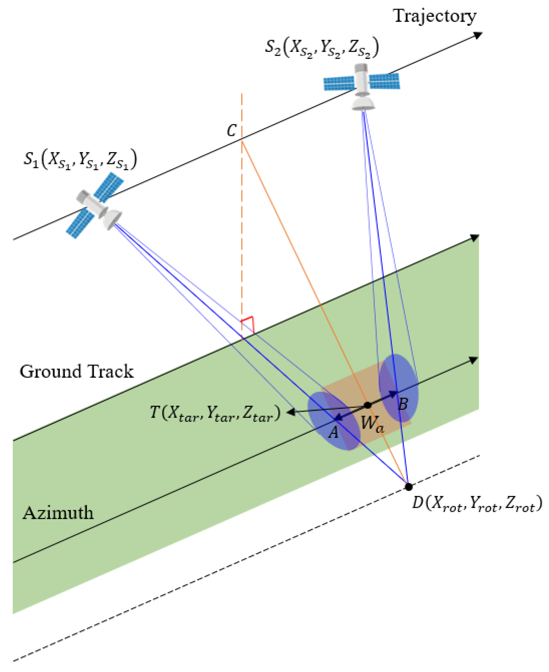
Since the SAR antenna is pointed to the center of rotation under the ground in sliding spotlight mode, the position of the center of rotation must be obtained in addition to the coordinates of the target and the satellite to analyze the attitude maneuvering. Figure 10 shows the position of the satellite, the position of the target (), and the position of the center of rotation () at the start point () and end point () of imaging to obtain the center of rotation when imaging the target in sliding spotlight mode. Each position is indicated based on the ECEF coordinate system.
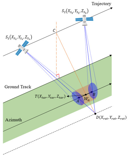
Figure 10.
Steering target when satellite points toward the rotation center.
If the position at the start of imaging is known, the position at the end of imaging can be obtained using the SAT calculated through Equations (19) or (24) in Section 2.3.2. If the four points are all in one plane, point becomes the midpoint of the points and is derived as shown in Equation (27).
Since the position of the target is known, we can find the position in the ECEF coordinate system using Equation (26) and then find the distance between the target and point . Additionally, since points are all in one plane and points and are on and , respectively, is in the same plane as , and at the same time, these have similarity. Therefore, the distance between the target and the center of rotation () can be obtained using the proportional equation, and the proportional equation is derived as in Equation (28), where the length of is equal to the swath width.
Since position (), the center of rotation in the ECEF coordinate system passes through point and is on a straight line parallel to the direction of . It can be obtained through the equation of the straight line, as shown in Equation (29).
In Phase 1, the vibration during imaging should be minimized to maintain image quality. For this, the characteristics of the satellite’s flexible structure must be considered even in Phase 1 maneuvering. In order to minimize micro-vibration applied to the satellite through structures such as flexible structure and CMG (Control Moment Gyro), the modeling including these details is required. In this study, a guidance profile was derived that minimizes the Doppler centroid variation according to the squint without reflecting the structural characteristic modeling.
2.4. Retargeting Maneuver and Optimal Retargeting Maneuver Time in Spotlight Mode (Phase 2)
2.4.1. Analysis of Optimal Retargeting Maneuver
To image continuous targets in the spotlight mode, the maneuvering must be performed to image the next target after imaging the previous target. In Phase 2, which is the retargeting maneuver section, since as many targets as possible in a single pass of the satellite must be imaged at the required resolution, it is necessary to minimize the retargeting maneuver time, as well as minimizing jerks that may cause mechanical vibration. In Phase 2, a profile for the actuator torque is required, and thus the approach to the dynamics problem will be needed. To solve this attitude maneuvering problem, the attitude motion equation of the satellite body, as shown in the following Equation (30), will be considered.
In Equation (30), is the torque received from the satellite, is the spacecraft’s inertia matrix, and is the angular velocity. To solve the maneuvering problem, the torque and angular momentum limit conditions that can occur in the actuator are considered. In this study, the analysis is performed by considering only the actuator torque, excluding external torques, such as gravity and drag. Torque is defined as . It is assumed that there exists only MoI without PoI (product of inertia). Therefore, , and if and are expressed, Equation (30) can be summarized as Equation (31).
Since the satellite body performs attitude maneuvering by the torque generated from the actuator, it can be optimized with the torque as the control input in Equation (31). In this analysis, GPOPS-II is used to optimize the retargeting maneuver time within the constraints. However, when optimizing using actual GPOPS-II, a control jitter problem may occur. In particular, if the infinite jerk type Bang-Bang control problem is defined, a torque input type profile that cannot actually occur to shorten the retargeting maneuver time and cluttering may be caused. This problem can be solved by creating a profile in the form of finite jerk. That is, the cluttering problem of the control input that may occur in GPOPS-II is solved by considering the jerk obtained by differentiating the torque as the control input. If is expressed as , and the actual control input can be expressed as Equation (32).
The retargeting maneuver can be optimized by using the attitude motion equation of the satellite body in Equation (31), the kinematic equation that calculated the quaternion in Phase 1, and the jerk control input in Equation (32). Through optimization, the quaternion during Phase 2 and the angular velocity of the satellite can be found. However, the norm problem may occur for the quaternion obtained through optimization. To solve this problem, the path constraint of quaternion is considered as Equation (33). The control input considered when performing the optimization in this study can be expressed as Equation (34).
In Figure 1, the final time free problem must be solved by using the quaternion and angular velocity of the satellite at the starting point of retargeting maneuver as initial values. This corresponds to the TPBVP, and to solve the problem, TPBVP must be defined as a problem having path constraints for final time free and final state to obtain a solution. The initial conditions and final conditions for optimization of retargeting maneuver can be summarized, as shown in Table 1.

Table 1.
Boundary conditions for retargeting maneuver.
Next, the constraints of the actuator consider the maximum and minimum values for the actuator torque, as shown in Equation (35).
The path constraints are defined by the constraints for solving the quaternion norm problem (see Equation (33)) and the angular momentum constraints that can be generated from the actuator as in Equation (36).
When the optimization through GPOPS-II is completed, the angular velocity and quaternion of the satellite at , which is the end point of the retargeting maneuver, can be calculated, and the history of input torque and angular momentum during the retargeting maneuver can be obtained. In the case of retargeting maneuvers for subsequent targets, the quaternion and angular velocity of the satellite at the end of the imaging section in Phase 1 of the relevant segment are used as initial values to optimize within the required control input and actuator constraints.
2.4.2. Analysis of Optimal Maneuvering Time in the Retargeting Maneuver
In this study, the objective function to be minimized should be determined for the optimization of retargeting maneuver. The shorter the retargeting maneuver time (RMT), the more images can be taken within a single pass, so the RMT is set as the objective function. However, simply minimizing the RMT can create a large jerk. Even if the next target is pointed quickly, it may take a long time to stabilize by the vibration caused. Therefore, even if the RMT increases slightly, the jerk must also be included in the objective function to achieve a stable pointing by reducing the occurrence of the jerk. The objective function is defined as a single objective function problem, as shown in Equation (37), by combining the RMT and the jerk.
In Equation (37), it is possible to determine which factor to focus more on minimizing by weighting each term of the objective function. and are constants, and the larger the values are, the smaller the change in the objective function, according to the change of the and values, so they do not have a significant effect. After all, it is necessary to optimize the objective function by substituting an appropriate constant.
2.4.3. Optimization Algorithm of the Retargeting Maneuver
It is possible to choose between the direct method and indirect method to generate the profile for optimal maneuvering. The direct method discretizes the attitude and control input of the satellite to find a solution, and it is easy to apply several constraints to the model. However, since the direct method may cause jitter of the control input, a solution that is difficult to apply to the actual problem may be derived. The indirect method is a form of solving TPBVP according to the Pontryagin Minimum Principle, and it can obtain accurate results compared to the direct method but has a disadvantage in that it is difficult to consider various constraints.
In this study, we simulated the optimization problem using GPOPS-II (General Purpose Optimal Control Software) [13], which is a direct method. GPOPS-II was originally developed for planetary exploration, orbit control, and attitude control optimization problems. GPOPS is a tool that can analyze multi-stage trajectory and is a suitable analysis tool for solving the optimal path problem. In GPOPS, the optimization problem can be solved using SNOPT (Sparse Nonlinear OPTimizer)/IPOPT (Interior Point OPTimizer), and in this paper, IPOPT [20] is used as the optimization algorithm.
SNOPT and IPOPT are software packages for large-scale nonlinear optimization. IPOPT is designed to find solutions of mathematical optimization problems and exploits 1st and 2nd derivative information using automatic differentiation routines or a quasi-Newton method. SNOPT employs a sparse sequential quadratic programming algorithm with limited-memory quasi-Newton approximation to the Hessian of the Lagrangian. IPOPT was selected in this research for easier use than SNOPT.
The general multiple-phase optimal control problem that can be solved by GPOPS−II should be defined as follows:
- -
- The cost function (i.e., performance index).
- -
- The continuous function (i.e., differential equations based on dynamics).
- -
- The time at the start and terminus of a phase.
- -
- The state at the start of a phase, during a phase, and at the terminus of a phase.
- -
- The control during a phase.
- -
- The path constraints.
- -
- The event constraints.
- -
- The static parameters.
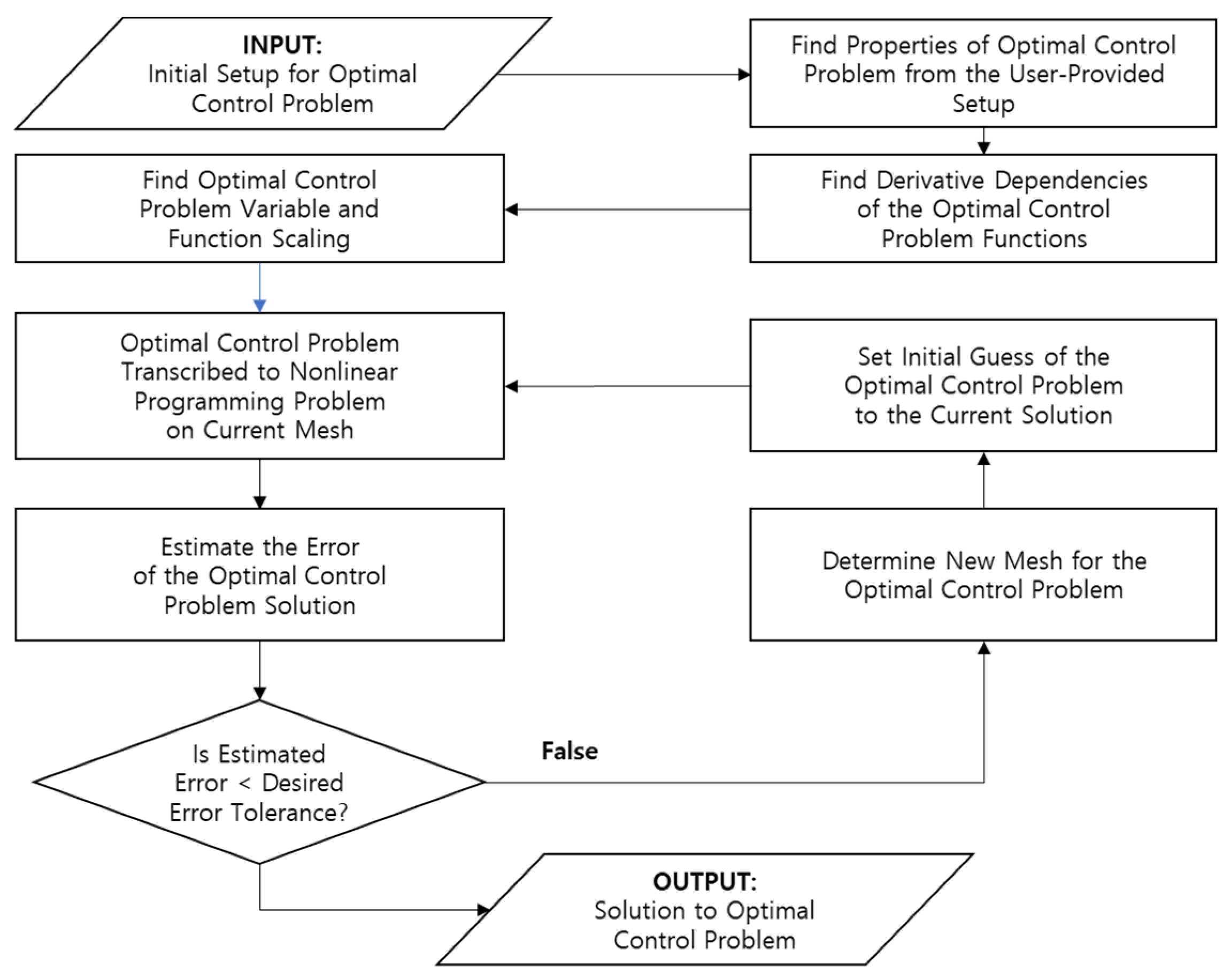
The optimization algorithm flow in GPOPS-II is shown in Figure 11.
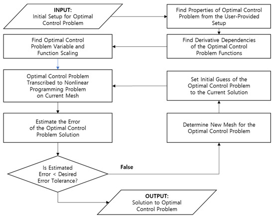
Figure 11.
GPOPS-II optimization algorithmic flow.
When using GPOPS-II, the upper and lower limits for the initial/middle/end states are set as inputs during the retargeting maneuver, as well as the time range between the initial and the end, the control input range, the maximum and minimum values of the path constraints, the setup of mesh, and an interpreter to perform optimization. In the imaging section (Phase 1), as described in Section 3.1, optimized maneuvering is not required, but in the retargeting maneuver section (Phase 2), there are many cases that can be maneuvered from the previous target to the next target. A case with the shortest retargeting maneuver time should be derived through optimization.
2.5. Development of Algorithm for Imaging Continuous Targets
In this study, based on the analyses in Section 2.3 and Section 2.4, we implemented an algorithm for analyzing the continuous target imaging scenario of passive SAR satellites using MATLAB. Figure 12 shows the flowchart of imaging for continuous targets, including attitude maneuvering and SAT in the imaging section of Phase 1 and the retargeting maneuver in Phase 2 and analysis of RMT.
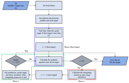
Figure 12.
Flowchart for the image-taking of successive targets.
First, target information (latitude and longitude), satellite coordinates, and velocity data for a single pass must be entered. At this time, the coordinates and velocity of the satellite are based on the ECEF coordinate system and are calculated based on the orbit dynamics. In addition, for the analysis of optimization for the retargeting maneuver, the MoI of the satellite, the constraints for the optimization, and the weighting of the objective function (see Equation (37)) are entered. When the analysis starts, the body frame of the satellite that minimizes the Doppler centroid variation is set through Equation (25). Through this, the squint angle formed with each target according to the coordinates of the satellite can be obtained. From the point when the squint angle, with respect to the first target, becomes the maximum required squint angle, the imaging (Phase 1) starts and the imaging maneuver analysis is performed.
Using the equation derived in Section 2.3, the SAT for the first target can be calculated. In addition, the angular velocity and attitude of the satellite used to continuously point toward the targets in the imaging section are calculated using the quaternion kinematic equation. After Phase 1 is over, the retargeting maneuver (Phase 2) to image the next target begins and the analysis is performed.
First, at the end of Phase 1, the quaternion and angular velocity of the satellite are entered as initial conditions to optimize the retargeting maneuver. After that, an optimal maneuver that can minimize the objective function of Equation (37) within the constraints is derived through GPOPS-II. When optimization is complete, the input data required for Phase 1 analysis of the next target are stored. At the beginning or end of imaging, the analysis of Phase 1 to Phase 2 is repeated until the squint angle is less than the minimum required squint angle, so that imaging is not possible or there are no more targets to image.
3. Simulation and Results of Target Imaging
3.1. Targets Arrangement Scenario and Simulation Parameters
Table 2 shows simulation parameters for optimal analysis of maneuvering during the imaging maneuver (Phase 1) and the retargeting maneuver (Phase 2). The analysis is performed by assuming that the MoI of the satellite is and the PoI is set to be 0 for that simplified simulation based on reflector antenna-based passive SAR satellite configuration. CMG is implemented to generate a torque of and an angular momentum of , and the analysis is performed by assuming that the altitude of the satellite is 570 km and the angle of inclination is 45°. The stabilization time is assumed to be 2 s in consideration of these unpredictable factors. SAR satellites use the frequency bandwidth of the X-band to obtain high resolution. The operating frequency of the X-band SAR satellite is assumed to be 9.6 GHz, and the wavelength is about . The margin of SAR SAT is considered as 25%. The constant values and of the objective function to be minimized in Equation (37) in Section 2.4.2 use 1sec and 100 rad2/sec5, respectively. By selecting and appropriately, we can determine which of the RMT or jerk occurrences should be minimized. If is increased, the change in according to becomes smaller, and has a greater effect on minimizing the objective function than . Therefore, the optimization is performed so that has a smaller value. Conversely, if is increased, the change in the value of becomes smaller, so that the has a greater effect on the change of the objective function. Therefore, it is optimized so that has a small value. In the case of , it is set as 1 while the number of RMT is less than 10 s, and in the case of , when the optimization is performed by substituting various values, a value of about 100 to 500 rad2/sec5 is obtained when calculating . We make sure that the difference between the possible values of and is not large. In addition, since it is more important to reduce the RMT as the section in which an image can be imaged is limited, in order to increase the change in , according to , is set to 100 rad2/sec5, so that the jerk and have a similar effect for the minimization of the objective function. Table 2 summarizes the simulation parameters assumed for this analysis.
Table 2.
Simulation parameters.
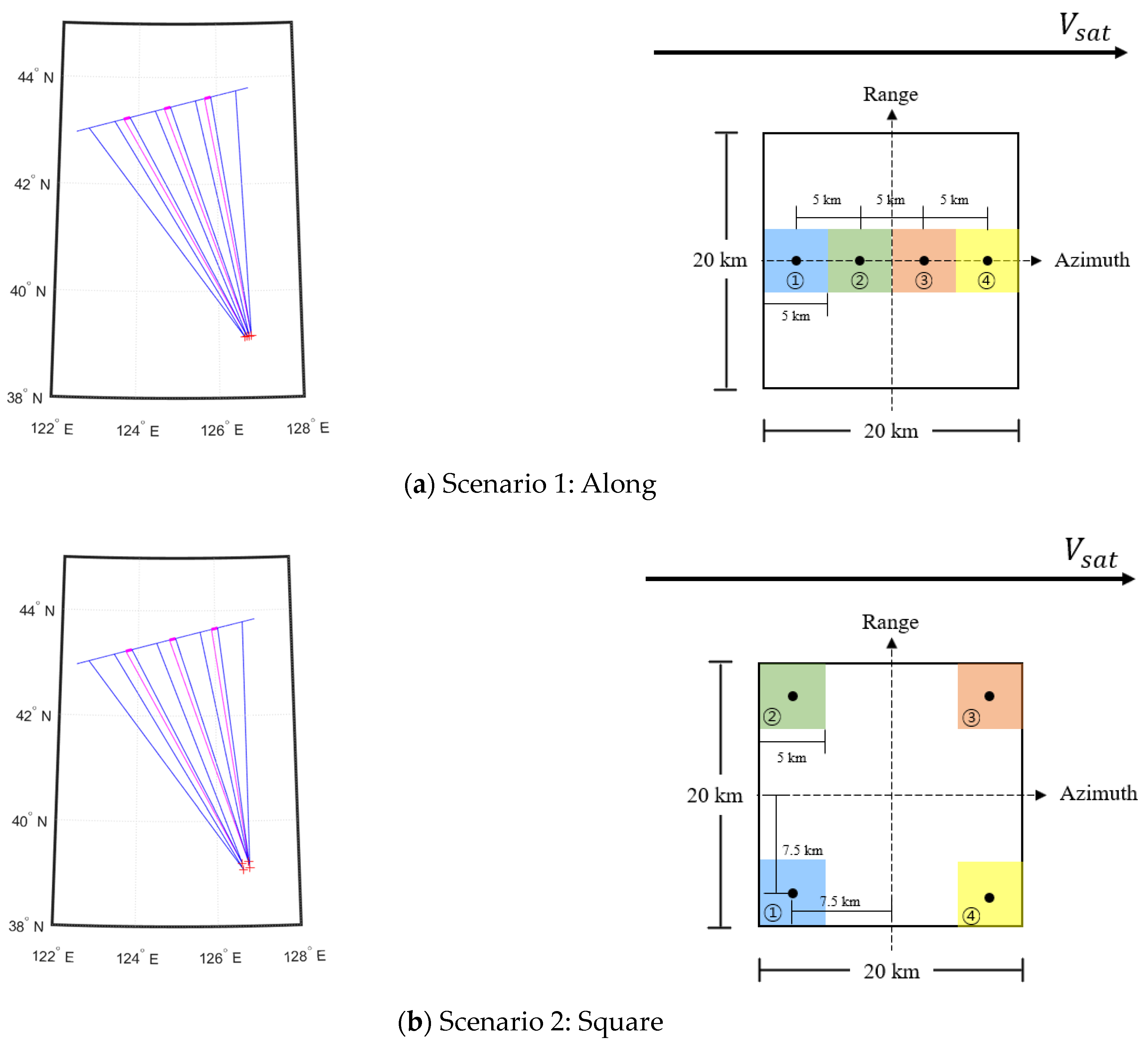
In general, when analyzing imaging capabilities within a wide AoI, it is an aim to take as many images as possible using mission planning/scheduling for multiple targets in a single pass. In this study, two target deployment scenarios are assumed to image a densely populated area of 20 km 20 km, as shown in Figure 13, for optimal analysis of imaging and retargeting maneuvers. It is assumed that images are taken in sliding spotlight mode to obtain images of four arbitrary 5 km 5 km targets in high resolution within the AoI of a densely populated area. To analyze the image-taking capability in a worst-case scenario through maneuvering between imaging and optimal retargeting maneuvers, we analyzed whether four targets could be imaged in a single pass using the squint mode imaging at the center of the AoI and at an angle of incidence of 45°. In the first scenario, four targets were arranged in a row (along), parallel to the direction (Azimuth direction) of the satellite. In the second scenario, the four targets to be consecutively imaged were arranged at the corner of the densely populated area (square). Optimization simulation was performed for the two scenarios defined above. As shown in Figure 13, a number was assigned to each target in each scenario, and then the imaging sequence was determined to provide a squint angle of 12° from the first target, and the squint angle was less than −12° when imaging of the last target was finished. In each scenario in this way, the imaging sequence with the shortest total time was determined among cases that were not less than −12° and analyzed as follows in Section 3.3. Considering image position accuracy in actual imaging, it is impossible to image the entire area of 20 km × 20 km while imaging four targets. However, in this study, it was assumed that there is no image position error when imaging.
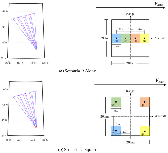
Figure 13.
Target scenarios for maneuvering simulation.
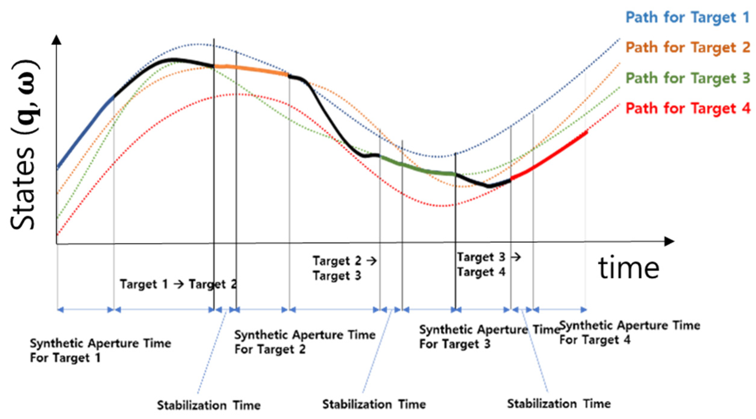
Attitude steering was created to minimize Doppler centroid variation for each target, and the corresponding trajectory was used as the initial and ending values of Phase 2 of each segment during the retargeting maneuver, and this concept is shown in Figure 14. Figure 14 shows the target path according to each target placement, the SAT including maneuvering during imaging, the RMT to the roll, pitch, and yaw axis, and the stabilization time in sequence.
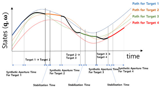
Figure 14.
Maneuvering simulation scenario.
3.2. Verification of Optimization Algorithm
By assuming the conditions of the two targets, as follows, it was examined whether the problem could be solved. The results of analysis using GPOPS-II based on IPOPT are as follows. First, it was checked whether the convergence to the optimum point was observed according to the constraints on the control input, the constraints on the state, and the optimization algorithm, and it was confirmed that the relative error gradually decreased each time the mesh was redefined. It was verified that the defined problem was solved as an optimization problem by GPOPS-II.
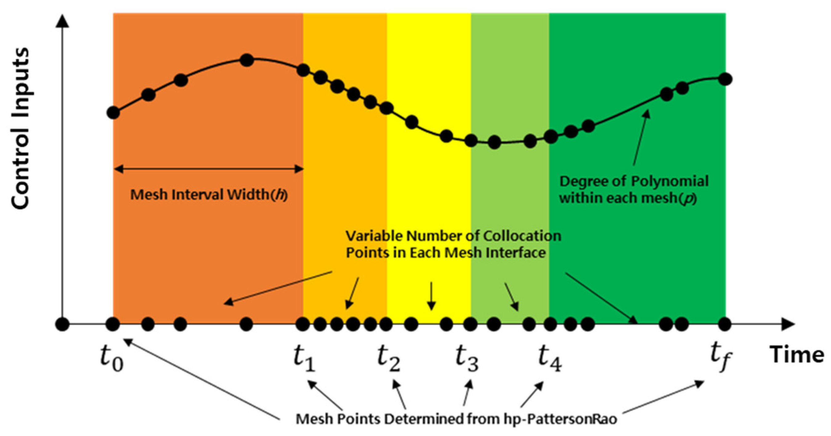
In this problem, the mesh and the collocation points within the mesh were redefined by hp-PattersonRao [21], and the concept of redefinition of the mesh and intra-mesh collaboration by hp-PattersonRao and the algorithm used in GPOPS-II is shown in Figure 15. The mesh and intra-mesh collocation continues to be redefined until the required error level is satisfied. The algorithm first seeks to increase the order of the approximating polynomial on a given interval to satisfy a specified tolerance and only subdivides the interval if the polynomial degree cannot be further increased.
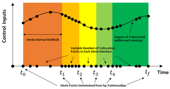
Figure 15.
Conceptual scheme of a hp-PattersonRao on GPOPS-II.
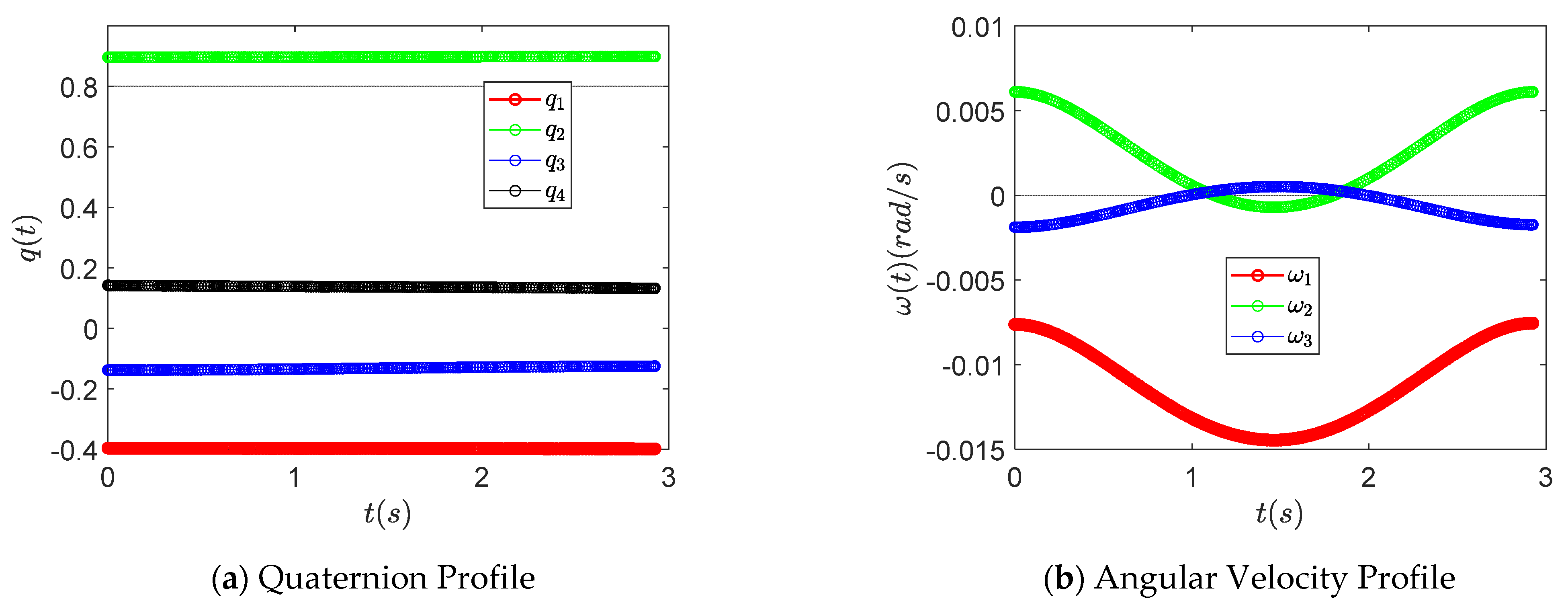
As an initial value for verification, quaternion is [−0.396, 0.896, −0.138, 0.142] and angular velocity is [−0.436, 0.350, −0.108] rad/sec. In this verification simulation, MoI is assumed to be [1000, 700, 500] kgm2 for the general demonstrative case. It can be confirmed to normally track according to constraints for final targets through Figure 16.

Figure 16.
State profile for end points verification of simple problem.
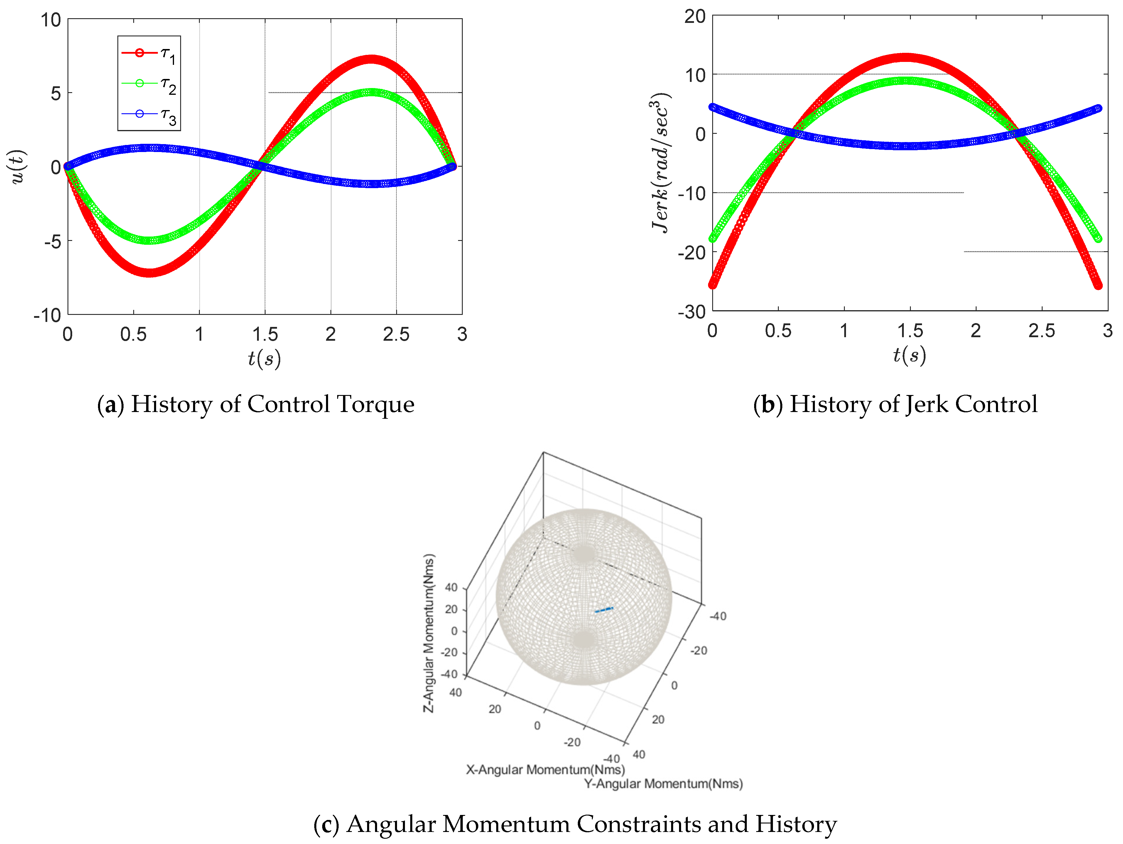
Figure 17 shows the torque and jerk control input for each axis and also illustrates the change of the angular momentum. It was confirmed that the result of satisfying the limiting condition for the torque magnitude for the torque control input and the result of satisfying the limiting condition of each momentum were achieved.
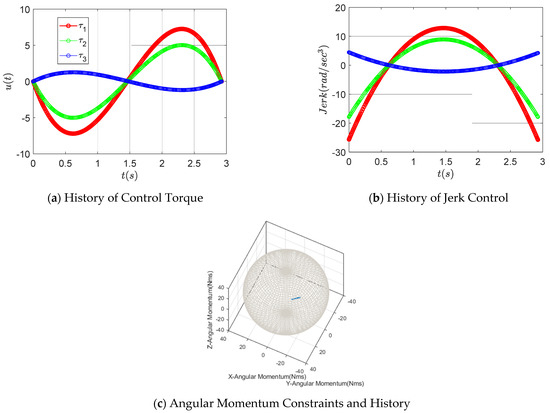
Figure 17.
History of control for retargeting control optimization.
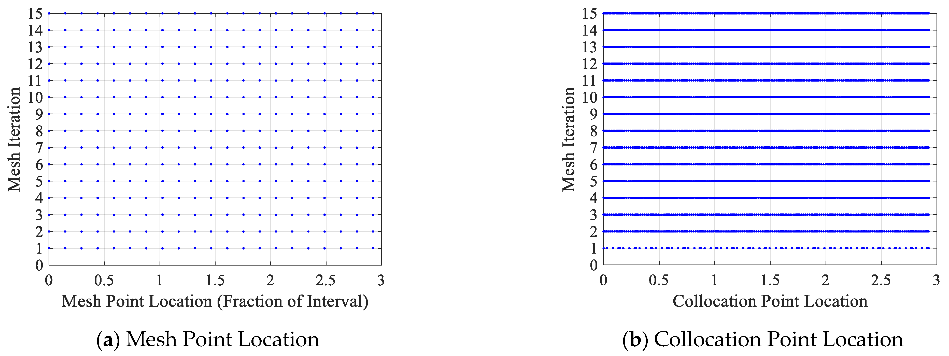
Figure 18 shows the change of the mesh points and the collocation points within the mesh each time the mesh was redefined according to the concept shown in Figure 15.
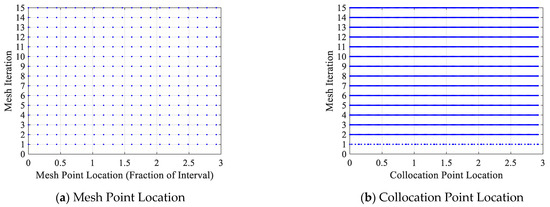
Figure 18.
History of mesh point location and collocation point location for retargeting control optimization.
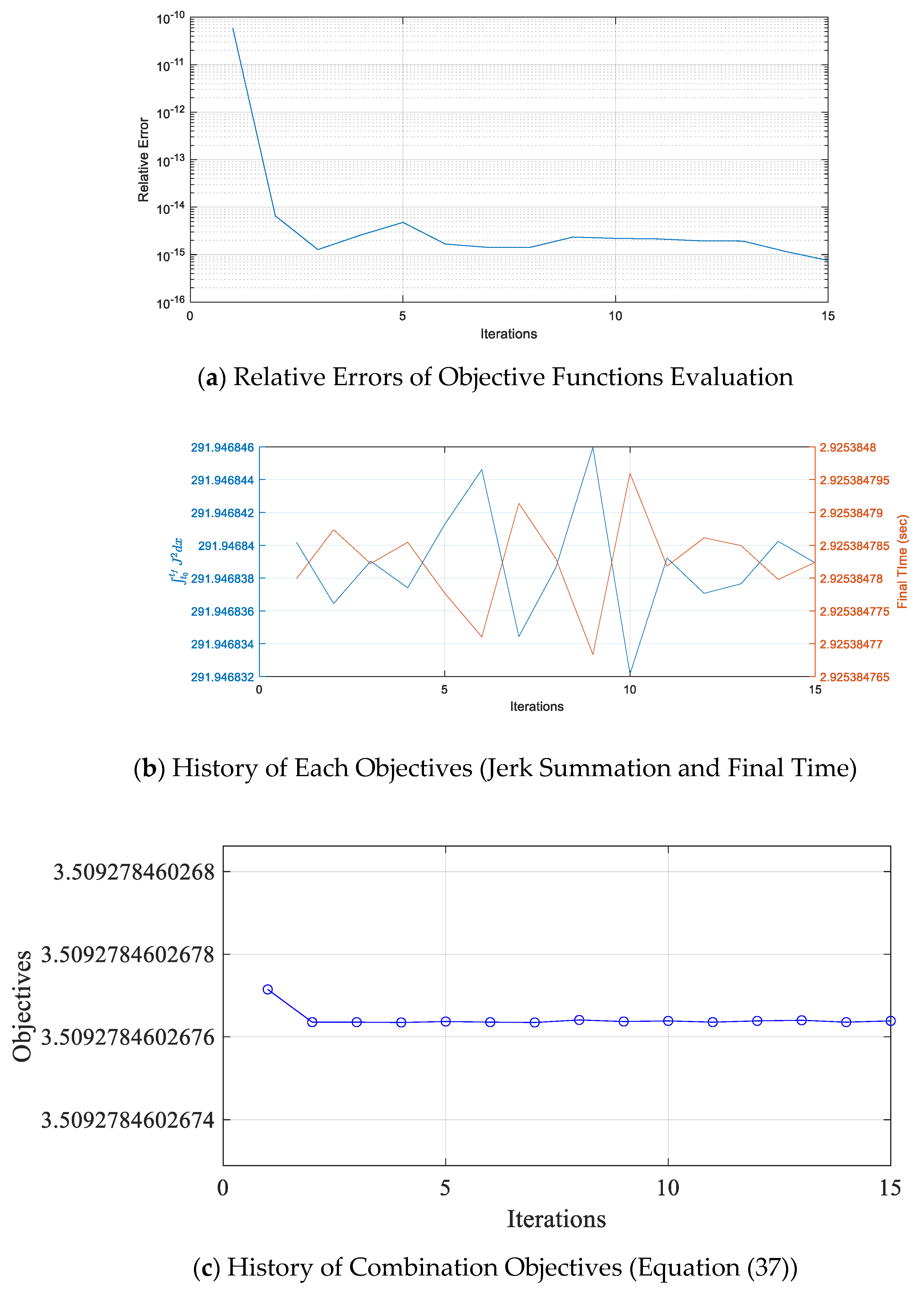
For mesh redefinition, the change of the relative error every time the calculation was repeated is shown in Figure 19a, and the change of the defined objective function is shown in Figure 19c. From Figure 19a, it was confirmed that the relative error satisfies 10−15 or less. In addition, as shown in Figure 19b, the final time and the integral values of jerk were mutually traded off. This means that the scale value was normally reflected. Two objective functions were expressed as Equation (37), and the trade-off for two objective functions was performed through repetitive computation. Finally, the GPOPS solver found an optimal solution to minimize the performance index expressed as Equation (37). The reason that relative errors were repetitively increased and decreased, as shown in Figure 19a, is due to the trade-off of two objective functions.
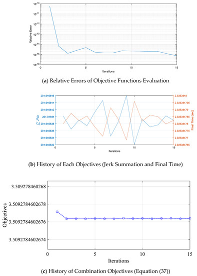
Figure 19.
History of objectives for retargeting control optimization.
3.3. Results of Simulation Analysis
Two scenarios were analyzed, as defined in Section 3.1, by executing the developed MATLAB code to analyze attitude maneuvering and maneuvering time in the imaging maneuver section and the retargeting maneuver section defined for continuous target imaging. Changes in quaternion, satellite angular velocity, angular acceleration, and squint angle over time during the mission were shown, and optimal control of retargeting maneuvers was analyzed using GPOPS-II software.
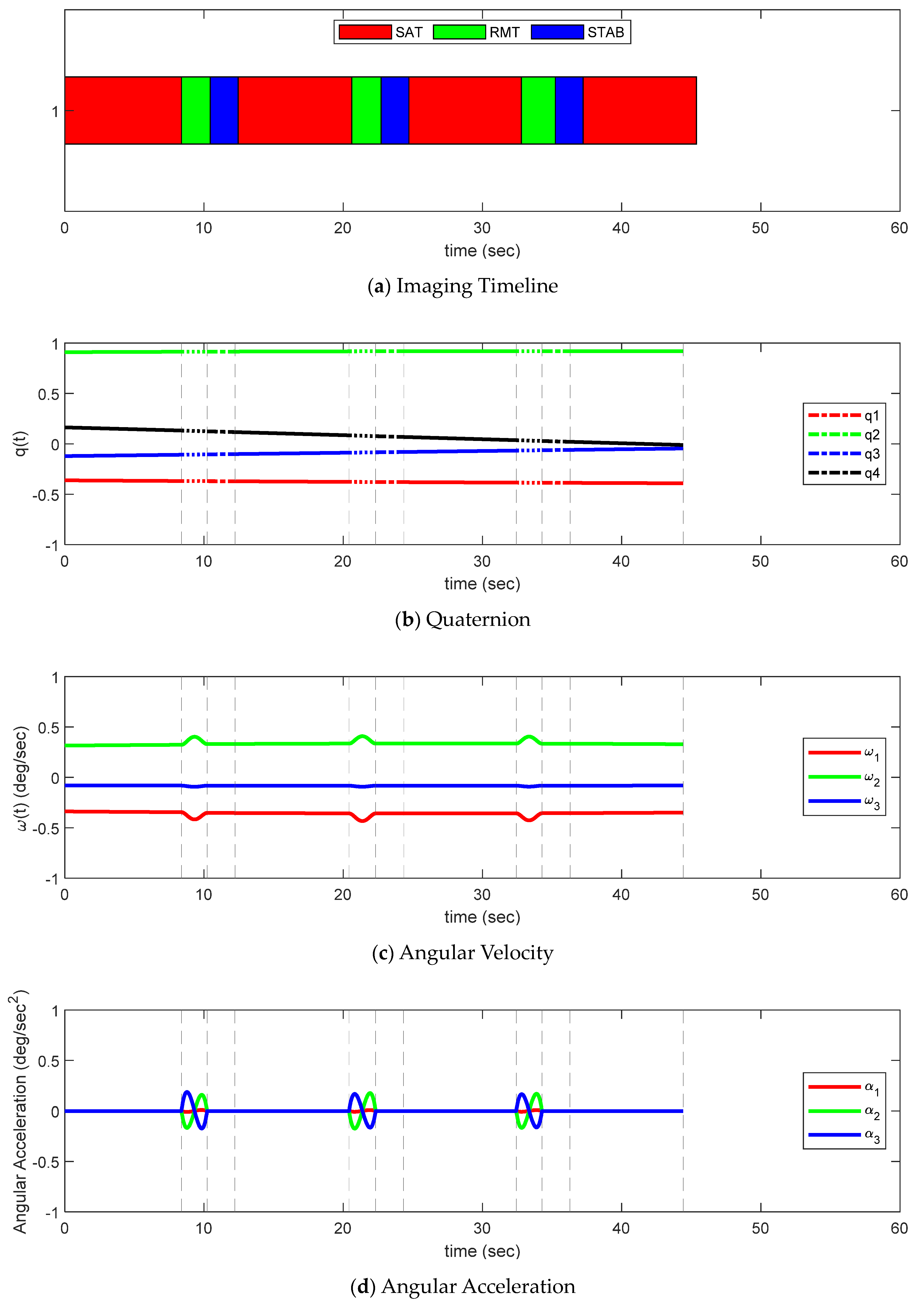
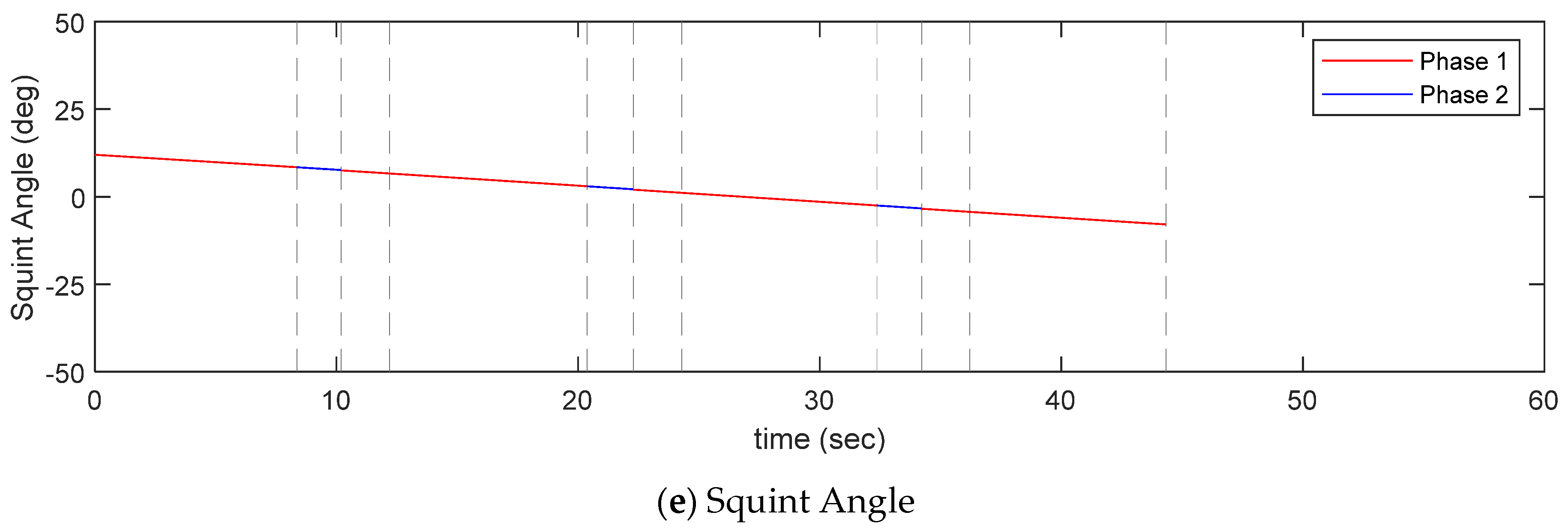
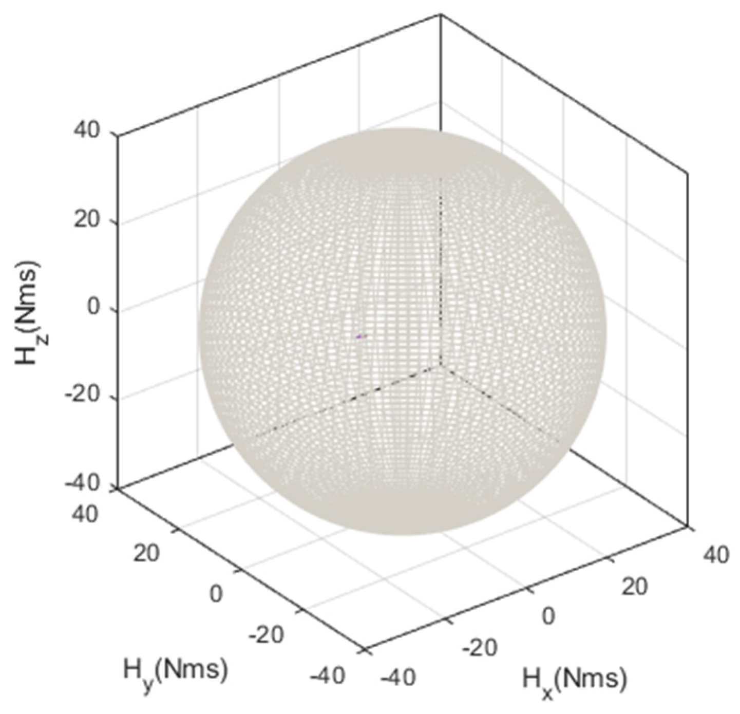
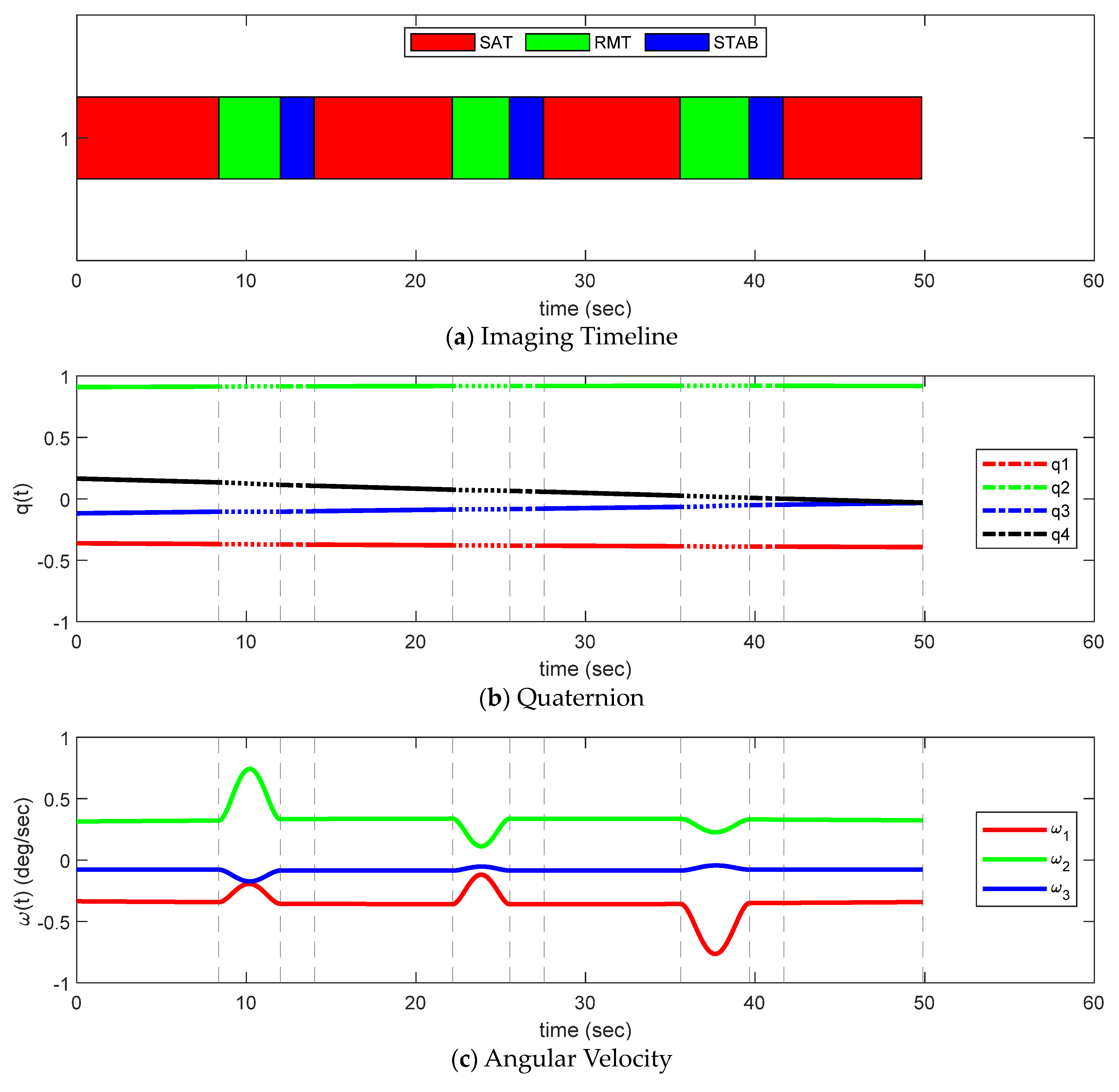
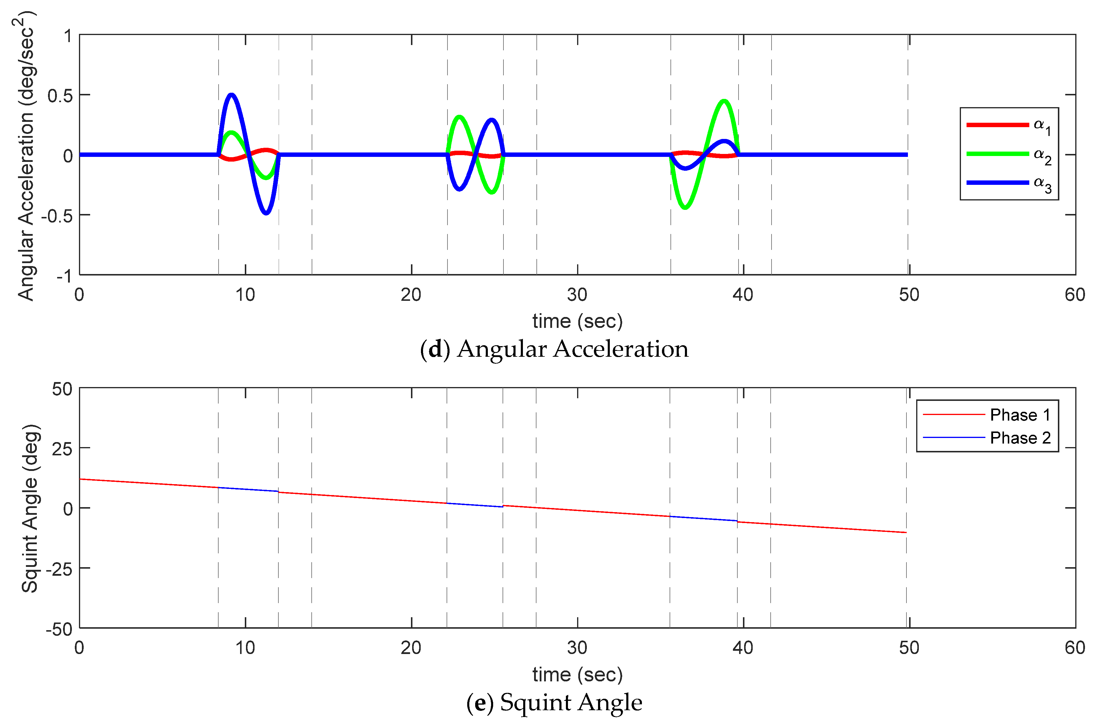
Figure 20 shows the timeline of quaternion, angular velocity, angular acceleration, squint angle change, and SAT, RMT, and stabilization time between continuous targets during the image-taking mission obtained through the analysis of [Scenario 1]. The imaging sequence of four targets was obtained through mission planning, where the squint angle at the end of the mission was not less than −12° and the total time was the shortest. In Figure 13a and Figure 20a, it was obtained that imaging in the order of ①-②-③-④ had the shortest total time [22]. As shown in Figure 20a, the SAT in Phase 1 took about 8.08~8.38 s for all four targets (25% margin was considered). Since it was imaging a dense area, the SAT was relatively similar. It can be confirmed that the smaller the squint angle, the shorter the SAT. This is because the squint angle is larger when the satellite is imaging in sliding spotlight mode, therefore, it is father from the target, so it takes a longer time to obtain the same resolution. Additionally, considering the imaging sequence, since the distance between adjacent targets is the same, it can be confirmed that there was no significant difference in RMT. Figure 20c shows the change in the angular velocity of the satellite during the mission. In Phase 1 (imaging section), the angular velocity appeared constant but actually changed slightly. This means that, in Phase 1, the CMG created a slight torque. In [Scenario 1], the angular velocity of roll direction was almost constant, even during Phase 2 (retargeting maneuver section), because the targets were aligned with the moving direction of the satellite. Since the image was taken with squint sliding spotlight mode, the satellite was directed toward the rotation center below the Earth’s surface for imaging, and the position of the rotation center for each target moved from right to left in the reverse order of imaging. The negative angular velocity of pitch direction in Phase 2 was larger than in Phase 1 because the squint angle was smaller as the rotation center was to the left. Figure 20d shows the change in the angular acceleration of the satellite during the mission. Since the torque was slightly generated in the CMG during image-taking, and the angular acceleration appeared to be 0, but it actually had a very small value. In Phase 2, the torque was generated in the CMG to direct the next target, and the angular acceleration also changed with time. Figure 20e shows the change in squint angle with time. At the end of imaging, the squint angle was −7.92°, which was the smallest change in squint angle compared to other scenarios, and since the sum of the RMT was also the smallest compared to other scenarios, it can be confirmed that the mission execution time was the shortest. This seems to be because, in [Scenario 1], the targets maneuvered in the direction of Azimuth when imaging, and the targets were also placed in the direction of azimuth so that they could maneuver to the next target faster. Figure 21 is a graph showing the history of angular momentum for [Scenario 1]. Since the magnitude of the angular momentum operates within the envelope of all three axes, it can be confirmed that singularity did not occur in CMG.
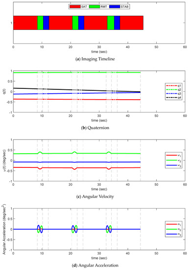

Figure 20.
Timeline/quaternion/angular velocity/angular acceleration/squint angle for Scenario 1.
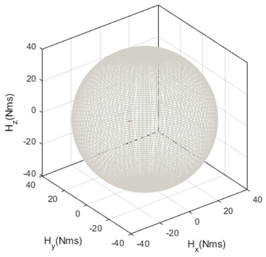
Figure 21.
Momentum history for Scenario 1.
Figure 22 shows the timeline of quaternion, angular velocity, angular acceleration, squint angle change, and SAT, RMT, and stabilization time between targets during the image-taking mission obtained through the analysis of [Scenario 2]. Through mission planning, imaging in the order of ①-②-③-④ in Figure 13b and Figure 22a satisfied the squint angle condition and resulted in the shortest mission execution time. As shown in Figure 22a, the SAT was almost like [Scenario 1], since the relative distance between targets was the farthest at 15 km and the RMT was relatively long. In addition, the distance from the maneuvering section between targets to the next target was all the same, but when retargeting the maneuver with the 2nd to 3rd targets, such as the rotation in only the azimuth direction without rotation in elevation direction, as in [Scenario 1], it was confirmed that the RMT was 3.37 s shorter than the RMT between other targets. Figure 22c shows the change in the angular velocity of the satellite during the mission. As in the case of [Scenario 1], in Phase 1, the angular velocity changed slightly, so the CMG generated torque slightly. In [Scenario 2], some targets were in slightly different positions in the roll direction, so the angular velocity of roll direction in Phase 2 changed more than in [Scenario 1]. However, since it was a target within a very dense area, the incidence angle for each target in [Scenario 2] was around 45°, and the squint angle during mission was within the range of ±12°. As a result, the angular velocity of the pitch direction became larger than that of roll direction in Phase 1 and Phase 2. When retargeting the maneuver from the 2nd target to the 3rd target, the targets were located parallel to the moving direction, as in [Scenario 1], but the decrease in the squint angle was relatively small because the distance between the targets were long. In the last Phase 2, since the rotation center was located to the left of the previous rotation center, the squint angle was more reduced and the negative angular velocity of pitch direction became larger than in Phase 1. Figure 22d shows the change in the angular acceleration of the satellite during the mission. Similar to [Scenario 1], a slight torque was generated in the CMG during image-taking and, accordingly, the angular acceleration changed with time. Figure 22e shows the squint angle change with time. The squint angle at the end of imaging was −10.26°, which was not the smallest angle compared to other scenarios, but it can be confirmed that the longest time was taken at 49.87 s when comparing the total mission execution time for each scenario. This is because the squint angle varies depending on the position of the target being imaged even if the satellites are in the same position.
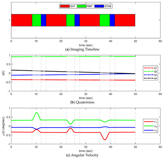
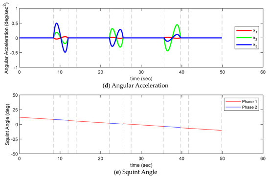
Figure 22.
Timeline/quaternion/angular velocity/angular acceleration/squint angle for Scenario 2.
Table 3 shows the SAT, RMT, stabilization time, and the time required to image four consecutive dense targets for the two scenarios. Although it was not published as a limit on the size of the paper, we analyzed other scenarios than the two assumed here in the same way as above. As a result of the analysis, [Scenario 1] is the best method in terms of imaging because the sum of the RMT is the shortest and the total time is also the shortest. Since [Scenario 2] has the longest total time, it can be judged as the imaging path of the worst case.
Table 3.
Comparison of imaging maneuver time, retargeting maneuver time, and stabilization time in four scenarios.
4. Conclusions
While active SAR satellites perform imaging through electronic beam steering, passive SAR satellites require higher agility performance during imaging because the satellite itself must maneuver to continuously point the targets. In addition, squint spotlight mode operation is required to improve imaging capability, but there have been few studies on attitude maneuvering. Squint spotlight mode operation is essential in order to image continuous targets in a single pass, and since the section in which image taking is possible for each target is limited, it is necessary to image more targets through an attitude maneuver that minimizes retargeting maneuver time.
In this study, we developed the software that derives the attitude maneuver when the passive SAR satellite performs imaging in the squint spotlight mode in a predetermined sequence to analyze the attitude maneuver and image-taking capabilities. The mission execution time of the satellite was analyzed by dividing it into an imaging section (Phase 1) and a retargeting maneuver section (Phase 2). In the imaging section (Phase 1), an equation to obtain the SAT of squint sliding and squint staring spotlight modes kinematically was derived, respectively, and compared with the characteristics of the attitude maneuver. In the retargeting maneuver section (Phase 2), because the attitude maneuvering is performed through the torque generated by the CMG, the attitude maneuvering and maneuver time of the satellite during the retargeting maneuver within the limited conditions were kinematically optimized using GPOPS-II.
To analyze the attitude maneuvering and imaging capability for the continuous target of the passive SAR satellite, two scenarios (Along, Square) were analyzed to image four 5 km × 5 km continuous targets within a 20 km × 20 km dense area. As a result of the analysis, it was confirmed that four targets can be imaged in high resolution when images are taken in squint sliding spotlight mode within ±12° of two scenarios. It was found that the along scenario has a shorter mission execution time through comparative analysis.
Based on this study, when imaging not only dense targets but also multiple targets scattered within the area of interest, it is possible to develop an attitude command generation software that can provide an optimized attitude maneuvering profile during the imaging period and the retargeting maneuver to image as many targets as possible in a single pass. In addition, the developed software is expected to be used for image collection planning in ground stations and for the development of attitude control module’s attitude command generation of satellite flight software.
The research results described in this paper are intended to create a guidance profile on the ground for feedforward onboard control, not a control algorithm used on spacecraft. Before transferring the guidance profile to the spacecraft from the ground, the feedforward control performance was analyzed by considering the orbit/attitude determination and attitude control error of the spacecraft. The analysis of post-processing performance was not the focus of this paper and is planned to be performed in future studies.
Author Contributions
Conceptualization, H.K. and Y.-K.C.; Methodology, H.K. and J.P.; Formal Analysis; J.P.; writing—original draft preparation, J.P., Y.-K.C. and H.K.; writing—review and editing, H.K. and Y.-K.C.; visualization, J.P. and H.K.; supervision, Y.-K.C.; project administration, S.-H.L.; funding acquisition, Y.-K.C. All authors have read and agreed to the published version of the manuscript.
Funding
This research was funded by the LIG Nex1 Corporation.
Institutional Review Board Statement
Not applicable.
Informed Consent Statement
Not applicable.
Data Availability Statement
The data used to support the findings of this study are available from the corresponding author upon request.
Acknowledgments
This research has been performed under the cooperation between Korea Aerospace University and LIG Nex1 Corporation.
Conflicts of Interest
The authors declare no conflict of interest.
Nomenclature
| Abbreviations | |
| AoI | Area of interest |
| CMG | Control moment gyro |
| DCM | Direction Cosine Matrix |
| ECEF | Earth center Earth fixed |
| GPOPS-II | General purpose optimal control software-II |
| LVLH | Local vertical local horizontal |
| MoI | Moment of inertia |
| PoI | Product of inertia |
| RMT | Retargeting maneuver time |
| SAA | Synthetic aperture angle |
| SAL | Synthetic aperture length |
| SAR | Synthetic aperture radar |
| SAT | Synthetic aperture time |
| TPBVP | Two points boundary value problem |
| Notation | |
| Quaternion of satellite | |
| Angular velocity of satellite [rad/sec] | |
| , | Initial & final quaternions of -th target during imaging maneuver, respectively |
| , | Initial & final angular velocity of -th target during imaging maneuver, respectively [rad/sec] |
| , | Initial & final squint angle of -th target during imaging maneuver, respectively |
| Initial roll/pitch/yaw angle of -th target during imaging maneuver [deg] | |
| Final roll/pitch/yaw angle of -th target during imaging maneuver [deg] | |
| Initial roll/pitch/yaw rate of -th target during imaging maneuver [rad/sec] | |
| Final roll/pitch/yaw rate of -th target during imaging maneuver [rad/sec] | |
| , | Initial & final quaternion of -th target during retargeting maneuver, respectively |
| , | Initial & final angular velocity of -th target during retargeting maneuver, respectively [rad/sec] |
| , | Initial & final squint angle of -th target during retargeting maneuver, respectively [deg] |
| Initial roll/pitch/yaw angle of -th target during retargeting maneuver [deg] | |
| Final roll/pitch/yaw angle of -th target during retargeting maneuver [deg] | |
| Initial roll/pitch/yaw rate of -th target during retargeting maneuver [rad/sec] | |
| Final roll/pitch/yaw rate of -th target during retargeting maneuver[rad/sec] | |
| Position of -th target at sliding spotlight mode [Latitude, Longitude] | |
| Position of satellite at point A in ECEF frame [km] | |
| Moment of inertia [kg m2] | |
| Torque of CMG [ Nm] | |
| Max torque of CMG [Nm] | |
| Max angular momentum of CMG [Nms] | |
| Jerk of CMG [rad/sec3] | |
| Synthetic aperture time at broadside staring spotlight mode [sec] | |
| Synthetic aperture time at squint staring spotlight mode [sec] | |
| Synthetic aperture time at broadside sliding spotlight mode [sec] | |
| Synthetic aperture time at squint sliding spotlight mode [sec] | |
| Retargeting maneuver time [sec] | |
| Stabilization time [sec] | |
| Slant range at aperture center [km] | |
| Radius of Earth [km] | |
| Slant range from the rotation center to target area center at aperture center [km] | |
| Synthetic aperture angle [deg] | |
| Incidence angle at aperture center [deg] | |
| Look angle at aperture center [deg] | |
| , | Starting & ending squint angles of image-taking at staring spotlight mode [deg] |
| Antenna beamwidth [deg] | |
| , | Starting & ending squint angles of image-taking at sliding spotlight mode [deg] |
| Earth central angle [deg] | |
| Latitude of satellite [deg] | |
| Longitude of satellite [deg] | |
| Synthetic aperture length [km] | |
| Swath width of target area[km] | |
| Altitude of satellite [km] | |
| Velocity of satellite [km/sec] | |
| Azimuth resolution [m] | |
| Doppler bandwidth [Hz] | |
| Wavelength of synthetic aperture radar [m] | |
| Direction vector of the target from satellite | |
| Velocity vector of satellite in ECEF frame | |
| Objective function | |
| Initial time at retargeting maneuver [Modified Julian Date, GSFC] | |
| Final time at retargeting maneuver [Modified Julian Date, GSFC] |
References
- Naftaly, U.; Levy-Nathansohn, R. Overview of the TECSAR Satellite Hardware and Mosaic Mode. IEEE Geosci. Remote Sens. Lett. 2008, 5, 423–426. [Google Scholar] [CrossRef]
- L’Abbate, M.; Germani, C.; Torre, A.; Campolo, G.; Cascone, D.; Bombaci, O.; Soccorsi, M.; Iorio, M.; Varchetta, S.; Federici, S. Compact SAR and micro satellite solutions for Earth observation. In Proceedings of the 31st Space Symposium, Colorado Springs, CO, USA, 13–14 April 2015; pp. 1–17. [Google Scholar]
- Sanfourche, J.-P. ‘SAR-lupe’, an important German initiative. Air Space Eur. 2000, 2, 26–27. [Google Scholar] [CrossRef]
- Yokota, Y.; Okada, Y.; Iribe, K.; Tsuji, M.; Ando, A.; Kunii, Y. Newly developed X-band SAR system onboard Japanese small sat-ellite “ASNARO-2”. In Proceedings of the Conference Proceedings of 2013 Asia-Pacific Conference on Syn-thetic Aperture Radar (APSAR), Tsukuba, Japan, 23–27 September 2013; pp. 81–83. [Google Scholar]
- Farquharson, G.; Woods, W.; Stringham, C.; Sankarambadi, N.; Riggi, L. The Capella synthetic aperture radar constellation, EUSAR 2018. In Proceedings of the 12th European Conference on Synthetic Aperture Radar, Verband Deutscher Elektrotrchniker (VDE), Aachen, Germany, 4–7 June 2018; pp. 1–5. [Google Scholar]
- Faizullina, D.; Uetsuhara, M.; Takahira, R.; Murayama, J.; Katayama, M.; Onishi, S.; Yasaka, T. Attitude Determination and Control System for the first SAR Satellite in a Constellation of iQPS. In Proceedings of the 71st International Astronautical Congress (IAC), Dubai, United Arab Emmirates, 12–14 October 2020. [Google Scholar]
- Davidson, G.W.; Cumming, I.G. Signal Properties of Spaceborne Squint-Mode SAR. IEEE Transact. Geosci. Remote Sens. 1997, 35, 611–617. [Google Scholar] [CrossRef] [Green Version]
- Chang, C.Y.; Jin, M.; Curlander, J.C. Squint mode SAR processing algorithms. In Proceedings of the IEEE International Geoscience and Remote Sensing Symposium (IGARSS), Vancouver, BC, Canada, 10–14 July 1989; pp. 1702–1706. [Google Scholar]
- Wang, Y.; Zhimin, Z.; Yunkai, D. Squint spotlight SAR raw signal sim-ulation in the frequency domain using optical principles. IEEE Transact. Geosci. Remote Sens. 2008, 46, 2208–2215. [Google Scholar] [CrossRef]
- Vandewal, M.; Rainer, S.; Helmut, S. Efficient and precise pro-cessing for squinted spotlight SAR through a modified Stolt mapping. EURASIP J. Adv. Sig. Proc. 2006, 2007, 1–7. [Google Scholar]
- Mok, S.-H.; Bang, H.; Kim, H.-S. Analytical Solution for Attitude Command Generation of Agile Spacecraft. J. Korean Soc. Aeronaut. Space Sci. 2018, 46, 639–651. [Google Scholar] [CrossRef]
- Wie, B.; Weiss, H.; Arapostathis, A. Quarternion feedback regulator for spacecraft eigenaxis rotations. J. Guid. Control. Dyn. 1989, 12, 375–380. [Google Scholar] [CrossRef]
- Patterson, M.A.; Anil, V.; Rao, A. GPOPS-II: A MATLAB software for solv-ing multiple-phase optimal control problems using hp-adaptive Gaussian quadrature collocation methods and sparse nonlinear programming. ACM Transact. Math. Softw. 2014, 41, 1–37. [Google Scholar] [CrossRef] [Green Version]
- National Center for Geospatial Intelligence Standards. Spotlight SAR Sensor Model. Supporting Precise Geopositioning; NGA: Springfield, MA, USA, 2010. [Google Scholar]
- Mittermayer, J.; Richard, L.; Elke, B. Sliding spotlight SAR pro-cessing for TerraSAR-X using a new formulation of the extended chirp scaling algo-rithm, IGARSS 2003. In Proceedings of the 2003 IEEE International Geoscience and Remote Sensing Sympo-sium. Proceedings (IEEE Cat. No. 03CH37477), Toulouse, France, 21–25 July 2003; pp. 1462–1464. [Google Scholar]
- Boerner, E.; Lord, R.; Mittermayer, J.; Balmer, R. Evaluation of TerraSAR-X spotlight processing accuracy based on a new spotlight raw data simulator, IGARSS 2003. In Proceedings of the 2003 IEEE International Geoscience and Remote Sensing Symposium, Proceedings (IEEE Cat. No. 03CH37477), Toulouse, France, 21–25 July 2003; pp. 1323–1325. [Google Scholar]
- Omelyan, I.P. On the numerical integration of motion for rigid polyatomics: The modified quaternion approach. Comput. Phys. 1998, 12, 97. [Google Scholar] [CrossRef] [Green Version]
- Diebel, J. Representing attitude: Euler angles, unit quaternions, and rotation vectors. Matrix 2006, 58, 1–35. [Google Scholar]
- Zhao, S.; Deng, Y.; Wang, R. Attitude-Steering Strategy for Squint Spaceborne Synthetic Aperture Radar. IEEE Geosci. Remote Sens. Lett. 2016, 13, 1163–1167. [Google Scholar] [CrossRef]
- Pirnay, H.; Rodrigo, L.-N.; Lorenz, T.B. Optimal sensitivity based on IPOPT. Math. Program. Comput. 2012, 4, 307–331. [Google Scholar] [CrossRef]
- Patterson, M.A.; William, W.H.; Anil, V.R. A ph mesh refinement method for optimal control. Optim. Contr. Appl. Methods 2015, 36, 398–421. [Google Scholar] [CrossRef]
- Kim, H.; Chang, Y.-K. Optimal mission scheduling for hybrid synthetic aperture radar satellite constellation based on weighting factors. Aerosp. Sci. Technol. 2020, 107, 106287. [Google Scholar] [CrossRef]


Publisher’s Note: MDPI stays neutral with regard to jurisdictional claims in published maps and institutional affiliations. |
© 2021 by the authors. Licensee MDPI, Basel, Switzerland. This article is an open access article distributed under the terms and conditions of the Creative Commons Attribution (CC BY) license (https://creativecommons.org/licenses/by/4.0/).