An Effort to Use a Solid Propellant Engine Arrangement in the Moon Soft Landing Problem

Abstract

This paper presents a control design strategy for the soft-landing problem on the Moon using solid propellant engines (SPEs). While SPEs have controllability issues and issues relating to the fact that they cannot be restarted, they are characterized by their reliability, simplicity, and cost-effectiveness. Consequently, our main contribution is to tackle this disadvantage by formulating a 1-dimensional landing optimization problem using an array of SPEs in a CubeSat platform, which is analyzed for different numbers of engines in the array and for three types of propellant grain cross-section (PGCS). The engines and control parameters are optimized by a genetic algorithm (GA) due to the non-linearity of the problem and the uncertainties of the state variables. Two design approaches for control are analyzed, where the robust design based on the uncertainties of the variables shows the best performance. The results of Monte Carlo simulations were used to demonstrate the effectiveness of the robust design, which decreases the impact velocity as the number of SPEs increases. Using an arrangement of ten SPEs, the landing was at −2.97 m/s with a standard deviation of 0.99 m/s; using sixteen SPEs, the landing was at −2.04 m/s with a standard deviation of 0.48 m/s. Both have regressive PGCS.

1. Introduction

Throughout history, landing on a celestial body different from our planet has captured our imaginations. The first to accomplish this feat was the lander of the Luna program by the Soviet Union on 3 February 1966, called Luna 9. Luna 9 was the twelfth attempt at a soft-landing by the Soviets; it was also the first to transmit photographs from the lunar surface. The lunar surface was subsequently reached by Surveyor-I that was built by the National Aeronautics and Space Administration (NASA) and Jet Propulsion Laboratory (JPL) on 30 May 1966. Unlike the Soviet Luna landers, Surveyor was a true soft-lander with a throttled liquid propulsion system, and a large solid-propellant retro-rocket engine (that comprised over 60% of the spacecraft’s overall mass) in the center [1]. The Solid Propellant Engines (SPEs) were used on many of the past exploration missions for orbital and landing maneuvers. However, the maneuvers began to require more precision and control for the new landing missions, which increased the challenges and control requirements. Under this scenario, the SPEs present flight controllability issues since they are not re-ignitable and have a thrust defined by the geometry of the propellant grain cross-section (PGCS) [2].

Past missions have generated a set of propulsion system improvements that can now be applied to solid propellants. The Viking module featured a propulsion system based on a multi-nozzle engine arrangement, called the VLC-REA, or Viking Lander Capsule Rocket Engine Assembly [1,3]. The VLC-REA used liquid propellant in a complex nozzle configuration that demonstrated higher performance by replacing the operation of a single nozzle with an arrangement of nozzles. Then, the arrangement reduced the temperature reached in the structural walls and reduced the mass of the engines [4]. However, the MPF mission first investigated this feature in 1967 with a simplified model in order to improve the lander’s performance and reduce the total mass required. MPF used three SPEs as retro-rocket engines, which ignited simultaneously to decelerate. Then, an airbag system was used to prevent damage when impacting the surface of Mars at $12.5$ m/s. As the firing of the engines was simultaneous, an energy damping system was necessary to avoid impact damage since the SPEs cannot land smoothly if used in the traditional way. However, benefiting from the physical advantages of using an array of engines such as the VLC-REA and the MPF, it is proposed to independently control the ignition of each engine in the array, allowing greater control flexibility. Therefore, our project studies the feasibility of controlling the landing of a 12U CubeSat on the moon, which is based on the aforementioned characteristics of an engine arrangement, the miniaturization of technology, the versatility of CubeSats and their reduced complexity of development.

Currently, the large-scale space exploration that is projected for the coming years makes us rethink the use of SPE in space missions. Filippo Maggi et al. [5] examine the opportunities that might arise using SPE in future space activities, which can lower their costs with a simple propulsion system characterized by reliable operation, easy handling, safe storage, simplicity in health and safety protection procedures during propellant production, and simplicity in design and development. In this context, SPEs should have a central role in space exploration in the short and medium-term future. Additionally, the SPEs reduce the number of mechanical parts, such as valves, tanks, and electrical components for control, decreasing the mass and volume required by the propulsion system. Donald G. Chavers et al. [6] explain that every effort must be made to reduce the mass needed for the spacecraft in future exploration missions, in which we want to contribute with a proposal for a low-weight module with SPE and small dimensions. Accompanied by the technology miniaturization and advanced additive manufacturing, this allows for the consideration of small rovers and landers (<100 kg), where each component must use a reduced amount of volume. This consideration returns to the initial philosophy presented by the Mars Pathfinder (MPF) mission: an economic small lander that used three SPEs simultaneously to generate braking thrust on Mars [7].

Reducing the structural dimension presents a new opportunity for new space activities. H. Kalita et al. [8] propose a Lunar 27U CubeSat Lander based on a liquid propellant engine for soft landing. Christian D.Grimm et al. present new opportunities for small landing modules [9] with a description of past missions that used small landing modules. They present a landing method based on the Shell Lander concept to land on Phobos with low $\Delta v$ velocity and impact forces. However, a propulsion system is necessary for higher $\Delta v$ velocity missions such as moon landing. Another important advance in this matter is presented by the Japan Aerospace Exploration Agency (JAXA) with its 6U CubeSat lander called OMOTENASHI [10]. They propose to transport the module as a secondary payload on NASA’s Space Launch System (SLS) Exploration Mission 1 (EM-1) launch. OMOTENASHI consists of scientific instrumentation with a single SPE in the propulsion system, which is used to slow down the module in orbit and start descending. Then, the speed of the module decreases to a speed close to 30 m/s. As the SPE cannot be controlled and there are uncertainties in the position and ignition point, they employ three types of technology, namely, an airbag system, a crushable material, and epoxy filling. On the other hand, it has 2 commercial gaseous propulsion systems (MiPS-VACCO) to control the attitude of the module in flight and correct SPE uncertainties.

Despite the advantages mentioned above, SPEs have control problems in performing smooth movements during flight derived from uncertainties. Filippo Maggi et al. [5] describes that the specific impulse $I_{sp}$ of the SPE can vary by 10% of the estimated nominal value without considering the uncertainties and vibration of the engine that add a transient noise. This value can also be affected by environmental conditions, corrosion, and burn erosion. However, even having a smaller uncertainty in the specific impulse, the altitude and velocity of the lander also have uncertainties that affect the control of the ignition point in this type of engine. The uncertainties in these parameters are one of the main reasons (along with the fact that the propellant is not re-ignitable) why SPEs are not currently used for soft-landing. In this scenario, our hypothesis is that the required thrust can be divided into multiple thrusts generated by an SPE array. In addition, that the ignition sequence of these engines will decrease the impact speed under the hypothesis that the variations produced by an SPE can be corrected by the following thrust of an SPE. For this, it is necessary to design an independent control function for each engine.

1.1. Powered Descend Control

Previous work and analysis were conducted on the landing problem. The use of Pontryagin’s principle to find the optimal control on Moon landing was presented by [11,12]. They proposed a simple way to design a control function for optimal ignition control with constant thrust in one degree of freedom. Recently, the optimal pinpoint and soft-landing problem have been solved and reported by [13,14,15,16,17], among others. However, the analysis assumes the use of a propulsion system with a controllable thrust profile. This thrust profile can be controlled using liquid propellant engine (LPE) such as hydrazine, which has been used with different actuation technologies: the Throttlable method and Pulse Width Modulation (PWM) where the flow is controlled by valves [18]. However, SPEs are not controllable like LPEs. In contrast, SPEs have a pre-defined thrust profile that depends on the propellant grain cross-sections (PGCS).

The PGCS is the transverse geometry of a propellant grain that best represents the progression of the burning area, and it can be modeled mathematically according to D. P. Mishra [19,20] under certain stability criteria in the combustion chamber. The thrust of a determined PGCS can also be related to the specific impulse $I_{sp}$ of the propellant mixture and the analytical mass flow. However, analytical methods are usually based on static assumptions or the purpose of motor design only. That is to say, it is assumed that the combustion temperature is constant, and that the pressure does not change explicitly in time, but varies as a function of the rate of change of the burning area. Therefore, to find an optimal control function that satisfies the soft landing condition with the characteristics of the propellant, a thrust profile close to reality is required from the PGCS. Consequently, the delay time, action time, burn time, and dead time must also be added to the thrust profile of SPE to design an optimal control system. For this reason, in this work, we implement a different mathematical model that allows us to analyze the central points of this work: design an optimal control system that minimizes landing error and find the best SPE setting for a given specific boost, mass flow rate, action time, dead time, PGCS, and lag time.

A control function must be designed to demonstrate the effectiveness of soft landing with SPEs and find the best configuration of propulsion systems. Then, this must be evaluated with the dynamics of the system, the mathematical model of the thrust, and the type of PGCS. Similar to J. Meditch [11] and Apollo guidance [21], we proposed a control function as a polynomial solution, which is easy to program and quick to calculate. This control proposal is designed using two approaches: a classical design and a robust design using genetic algorithms (GA). GA has already proven to be an important tool for robust control design [22,23]. Yue Gao et al. [24] present an optimization formulated as a minimax problem so that system performance is optimized in the worst case of uncertainty. Their strategies integrate the objective functions of the subsystems to obtain a systematic optimization using a set of weights. However, in the landing problem, worst-case uncertainties do not necessarily lead to worst-case landings. The landing process is a non-linear process that must be considered as a set of cases within the uncertainties. In this context, a second approach is presented by Ivan Sekaj [25]. In his work, the cost function used in the robust design is the sum of all the sub-cost functions of a population of simulations carried out, where the populations differed by the standard deviation of the initial state uncertainties. This last one is the method used in our work.

1.2. Research Proposal

This paper presents a theoretical control design strategy for a SPEs array in a 1-dimensional soft landing problem. We propose that the array can divide the thrust required by the number of engines that are controlled independently. In this way, deviations in the optimal trajectory can be corrected by thrusts initiated at different control points. The engines considered are traditional combustion and ignition ones, which reduces the number of complex mechanical parts related to the liquid propellant engine, such as valves, tanks, and thermal systems, as well as electrical control components. The control function of each engine is designed assuming that it depends on the current altitude and speed of the module together with their respective gains. Control gains, the mass flow, and the action time of the engines are solved in an optimization problem to minimize the landing error by means of genetic algorithms (GA) due to the nonlinearity of the problem. Two different approaches are tested to solve the optimization, where the robust design approach is expected to deliver better results. For this, sixty landing cases are created by Monte Carlo simulations to evaluate the performance of the two approaches.

2. Problem Definition

Generally, the landing process is the stage where the module is controlled by the propulsion system to land at near-zero velocity at the target location. Landing in this place accurately is one of the main research challenges in the new generation of expensive space exploration missions. These missions, such as InSight and the Mars Science Laboratory (MSL), have a unique and expensive rovers and landers; therefore, they reduce risk by calculating the trajectory as accurately as possible. For lunar applications, accuracy is important to get close to interesting craters from a mining point of view or in the study of oxygen formation. According to Gustavo Jamanca-Lino [26], the production of oxygen on the moon is crucial for obtaining water, rocket fuel, and promoting commercial activities between the Earth and the Moon. In this sense, the focus of this research is not to improve the precision with respect to the state of the art but to present the effectiveness of using SPEs in the EDL process and to quantify the best precision achieved in soft-landing.

As previously stated, the SPE does not have the ability to be controlled in flight because it is not re-ignitable and has a predefined thrust profile with a constant action time $t_a$. These characteristics create an unstable environment for soft-landing control, which will be limited by a single ignition point. If the ignition point is not satisfied, additionally adding a variation of 10% in $I_{sp}$, the spacecraft leaves the optimal trajectory and the required soft-landing is not achieved. To tackle this problem, we separate the ignition process by using multiple ignitions of the arrangement of engines. This array divides the thrust and decreases the individual error of each engine. For example, if an engine working for a certain time does not have an optimal trajectory, the next engine working corrects the trajectory towards the optimal one. On the other hand, the multiple thrusts are analyzed for different numbers of engines and PGCS, which defines how the thrust profile behaves. Three principal PGCS known as Regressive, Neutral, and Progressive were simulated to find the best performance based on landing precision and a descent velocity bound.

To formulate a solution for using SPEs on the landing problem, we proposed a pseudo-landing module of low mass based on the CubeSat Design Specification (CDS). We detail more in the next subsection on the dimension and configuration of the engines. This strategy is an approach similar to the work presented by [8,10,27], where the electronic components are commercial CubeSat parts. Our propulsion system is based on an arrangement of SPEs that is symmetric to the vertical axis, as shown in Figure 1 and Figure 2. A one-dimensional coordinate system is used to present the effectiveness of the SPEs arrangement in a simplified scenario and to explain in more detail the results.

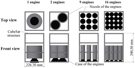
Figure 1. Example of 12U landers with engine arrangements. From left to right, 4 examples are shown: For a configuration of one, two, nine and sixteen engines.

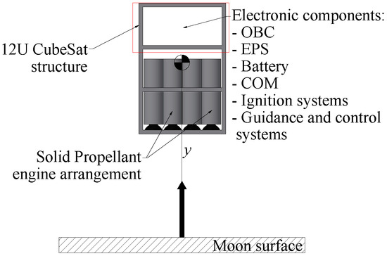
Figure 2. Example of a lander with 10 thrusters in the engine array in a one-dimensional dynamic model. The inertial reference frame is fixed on the lunar surface, and is perpendicular and positive to it. This configuration frees up space equivalent to 4U for electronic components.

2.1. Landing Module Description

The lander used is a 12U CubeSat structure dedicated to being the landing module, which has an engine arrangement. The engines are designed to use a maximum of 8 units (8U) below the structure, where they remain stored inside until the landing mission. Figure 1 shown a tentative engine array in the 12U structure.

2.2. Dynamic Model

According to the reference frames in Figure 2, the dynamic model during the landing process is defined as

$$\ddot{y}=g+\frac{T}{m}$$

(1)

$$\dot{m}=-T/v_e$$

(2)

where y is the altitude, g is the Moon gravitational acceleration, T and m are the thrust profile magnitude and mass module, respectively. The propellant exhaust velocity, $v_e$, is defined as $v_e=I_{sp}·g_e$, where $I_{sp}$ and $g_e$ are the specific impulse and earth gravity acceleration at zero altitude, respectively. The thrust, T, is defined by the summation of all solid propellants during flight, but we will detail this topic in the following subsection.

2.3. Thrust Description

Each engine has a predefined thrust profile that is derived from the PGCS. As part of the SPE array, these engines can be activated at different times, influencing the total thrust of the array. Then, the total thrust is defined as the sum of all engine thrust profiles working at a determinate time, and it has the ability to generate multi-level thrust magnitude $T\left(t\right)$. The total thrust generated by the arrangement of $N_e$ engines is

$$\begin{array}{cc}\hfill T\left(t\right)& =\sum _{k=1}^{N_e}{T}_k\left(t_k^{*}\right)\hfill \end{array}$$

(3)

where $T_k\left(t_k^{*}\right)$ is the thrust profile of each k-engine defined by the solid propellant burn area, and $t_k^{*}=t-t_{ig,k}$ is the current ignition time that start at the ignition time $t_{ig,k}$ for a given time t in the simulation.

To find the best performance of the thrust profile of each engine, we compared three different PGCS: Regressive, Neutral, and Progressive. These are related to star-regressive burning, tubes with rod-neutral burning, and star-progressive or tubular burning (BATES), in that order (see Table 1) [19,28]. According to this reference, the behavior of a particular star grain is defined by

$$\left[\left(\frac{\pi }{2}+\frac{\pi }{n_s}-\frac{\theta }{2}\right)-cot\frac{\theta }{2}\right]=0$$

(4)

where $n_s$ is the number of star points, and $\theta$ is the opening star point angle.

Table 1. Advantages and disadvantages of different PGCS.

Popular Types of PGCS	Advantages	Disadvantages
EndBurn (Neutral)	- Long action time	- Low thrust
	- Stable and neutral thrust	- The chamber wall must be thick (greater weight) due to direct and long exposure of high-pressure and high-temperature combustion gases
Star (Neutral, Progressive, and Regressive)	- The shape of the star can be modified depending on the thrust requirements	- Short action time
		- The shape is more difficult to manufacture compared to the others
BATES (Progressive)	- High final thrust	- Very low thrust at the start of ignition
	- Low weight	- Short action time

For a given $n_s$, the solution of the Equation (4) is called the neutral star grain angle, ${\theta }_{neutral}$. The star grain produces regressive burning when the design angle ${\theta }_d>{\theta }_{neutral}$, and regressive burning when ${\theta }_d<{\theta }_{neutral}$. We detail some advantages and disadvantages of the different PGCS in the Table 1 to contrast them in relation to the desired result.

In each type of PGCS, we assume that the engines have the same maximum thrust max$\left(T_k\right)$ and $I_{sp}$ in the arrangement. On the other hand, a mathematical model is used to describe each thrust profile of the PGCS, which is used in the optimization. These models are shown below, but in a real application, the experimental measure of thrust should be used.

2.3.1. PGCS-Regressive

The regressive thrust profile is modeled with a hyperbolic tangent function (HTF) at the beginning, a negatively sloping linear function in the middle, and again with an HTF at the end. The mathematical model for the unitary thrust $T_k\left(t_k^{*}\right)/max\left(T_k\right)$ is

$$\left\{\begin{array}{cc}\frac{\left(1 + tanh\left(\left(\frac{t^{*}}{{\tau }_d}-\zeta \right)s\right)\right)}{2}\hfill & t_k^{*}\le {\tau }_d+{\tau }_l\hfill \\ {\kappa }_r{t}_k^{*}+c_r\hfill & t_k^{*}\le {\tau }_r\hfill \\ \frac{\left(1 + tanh\left(\left(-\frac{\left(t_k^{*}-t_a-2{\tau }_d\right)}{{\tau }_d}-\zeta \right)s\right)\right)}{2}\hfill & t_k^{*}\le {\tau }_d+t_a+{\tau }_l\hfill \\ 0\hfill & otherwise\hfill \end{array}\right.$$

(5)

where ${\tau }_l$ is the lag time to reach 99.99% of the thrust, ${\tau }_d$ is the delay time to reach 10.0% of the thrust, and ${\tau }_r$ is the final point in the linear regression. The parameters ${\kappa }_r$, $\zeta$, s, and $c_r$ are calculated as

$$s=\frac{arctanh\left(f_1·2-1\right)-arctanh\left(q_{\%}·2-1\right)}{\left(\frac{\left({\tau }_l+{\tau }_d\right)}{{\tau }_d}-1\right)}$$

(6)

$$\zeta =1-\frac{arctanh\left(q_{\%}·2-1\right)}{s}$$

(7)

$${\kappa }_r=-\frac{f_1-f_2}{{\tau }_r-{\tau }_d-{\tau }_l}$$

(8)

$$c_r=f_1-{\kappa }_r\left({\tau }_d+{\tau }_l\right)$$

(9)

where $q_{\%}$ is the percentage of maximum combustion chamber pressure when the action time $t_a$ starts and ends according to [19]. For a $q_{\%}=0.1$ (typical value), the action time corresponds to $80\%$ of the total burning time.

We assume a maximum regression value of $99.9\%$ of the thrust ($f_1=0.999$), and a final value in the regressive curve of $30\%$ ($f_2=0.3$). Now, ${\tau }_i$ is defined as

$${\tau }_r=t_a+2{\tau }_d-\left(\frac{arctanh\left(2f_2-1\right)}{s}+\zeta \right){\tau }_d$$

(10)

Example: For an ignition time $t_{ig,k}=0$ of a single engine, ${\tau }_d=0.2$, ${\tau }_l=0.5$, $t_a=5$ s, the Equation (5) result in the thrust profile shown in Figure 3.

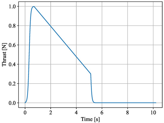
Figure 3. An example of regressive unitary thrust.

2.3.2. PGCS-Neutral

The neutral star grain (${\theta }_d={\theta }_{neutral}$) is used because of its advantages in order to increase the initial surface area [29] and to keep a semi-constant thrust. The typical thrust profile for the star design is a backward-neutral burn area. As the burning area progresses, its surface area decreases as the outer portion of the grain expands, exposing more surface area. This trade-off yields the thrust profile depicted in Figure 4. The mathematical model for the unitary thrust $T_k(t-t_{ig,k})/max\left(T_k\right)$ is

$$\left\{\begin{array}{cc}\frac{\left(1 + tanh\left(\left(\frac{t_k^{*}}{{\tau }_d}-\zeta \right)s\right)\right)}{2}\hfill & t_k^{*}\le {\tau }_d+\frac{t_a}{2}\hfill \\ \frac{\left(1 + tanh\left(\left(-\frac{\left(t_k^{*}-t_a-2{\tau }_d\right)}{{\tau }_d}-\zeta \right)s\right)\right)}{2}\hfill & t_k^{*}\le {\tau }_d+t_a+{\tau }_l\hfill \\ 0\hfill & otherwise\hfill \end{array}\right.$$

(11)

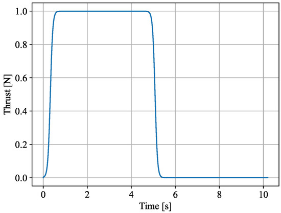
Figure 4. An example of neutral unitary thrust.

2.3.3. PGCS-Progressive

For progressive solid propellant, the BATES PGCS is the most widely known shape. The whole grain is in the shape of a solid cylinder with a circular hole in the center along the cylinder. Another progressive thrust is obtained by star-progressive. The progressive thrust is shown in Figure 5.

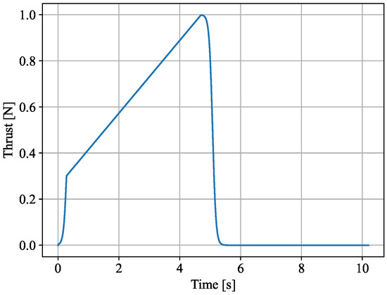
Figure 5. An example of progressive unitary thrust.

The mathematical model for the unitary thrust $T_k(t-t_{ig,k})/max\left(T_k\right)$ is

$$\left\{\begin{array}{cc}\frac{\left(1 + tanh\left(\left(\frac{t_k^{*}}{{\tau }_d}-\zeta \right)s\right)\right)}{2}\hfill & t_k^{*}\le {\tau }_p\hfill \\ {\kappa }_p{t}_k^{*}+c_p\hfill & t_k^{*}\le {\tau }_d+t_a-{\tau }_l\hfill \\ \frac{\left(1 + tanh\left(\left(-\frac{\left(t_k^{*}-t_a-2{\tau }_d\right)}{{\tau }_d}-\zeta \right)s\right)\right)}{2}\hfill & t_k^{*}\le {\tau }_d+t_a+{\tau }_l\hfill \\ 0\hfill & otherwise\hfill \end{array}\right.$$

(12)

where ${\kappa }_p=-{\kappa }_r$, ${\tau }_p$ is the starting point in the linear progression. ${\tau }_p$ and $c_p$ are defined as

$${\tau }_p=\left(\frac{arctanh\left(2f_2-1\right)}{s}+\zeta \right){\tau }_d$$

(13)

$$c_p=f_2-{\kappa }_p{\tau }_p$$

(14)

2.4. Boundary Conditions

The initial condition is defined by

$$\begin{array}{c}\hfill y\left(0\right)=y_{0}m,v\left(0\right)=0m/s,m\left(0\right)=m_{0}kg,\end{array}$$

(15)

and the desired final condition is

$$\begin{array}{cc}\hfill y\left(t_{land}\right)=& y_{land}=0m\hfill \\ \hfill v\left(t_{land}\right)=& v_{land}=0m/s\hfill \\ \hfill m\left(t_{land}\right)=& m_{land}\left(free\right)kg,\hfill \end{array}$$

(16)

where $t_{land}$ is the time when the module first touches the surface. To estimate this value, it is important to note that due to the discretization of the simulation, the value closest to zero will be considered as the final point of contact with the surface. That is, if at time $t_k$ the height is $y_k=0.2m$ and the position at time $t_{k+1}$ is $y_{k+1}=-0.1m$, it is considered as final surface contact the value $-0.1m$, and the landing time is $t_{k+1}$.

2.5. Uncertain Parameters

There are three categories of groups where unknown parameters are found as disturbances. Each of them is briefly detailed below.

2.5.1. Altitude and Velocity

The initial altitude and velocity of the system will always have an uncertainty component derived from sensors, mathematical models, and/or estimation filters. This uncertainty is translated into a range of unknown parameters. That is why, in the initial physical conditions, we will assume Gaussian noises, such that

$${\widehat{y}}_0=y_0+\mathcal{N}(0,{\sigma }_{alt}),{\widehat{v}}_0=v_0+\mathcal{N}(0,{\sigma }_{vel}).$$

(17)

Here, ${\sigma }_{alt}$ and ${\sigma }_{vel}$ are the standard deviations for altitude and velocity, respectively.

2.5.2. Specific Impulse with Bias and Noise

As mentioned in the first section, the value of the specific impulse of a certain propellant can vary by up to $10\%$ from the theoretical one [5]. Therefore, the $I_{sp,k}$ of each engine will be updated once as expressed below.

$$I_{sp,k}=I_{sp}+\mathcal{N}(0,{\sigma }_{bias})$$

(18)

The standard deviation, ${\sigma }_{bias}$, is calculated as follows.

$${\sigma }_{bias}=\frac{I_{sp}·10\%}{gf}$$

(19)

where $gf$ is a factor which is selected in function of the desired percentage within the distribution, as shown in the Table 2. For this analysis, the parameter $gf=3$ was selected.

Table 2. Percentage within the distribution concerning $gf$.

gf	Confidence Interval	Percentage within the Distribution
1	+1 s	68.27%
2	+2 s	95.45%
3	+3 s	99.73%

Now, a noise signal corresponding to an erosive burn, humidity condition, and internal burning zone has been added. We assume that the noise has the same Gaussian distribution as before, and its new mean value is the $I_{sp,k}$ calculated by the last subsection. The ${\sigma }_{noise}$ is represented by the $3\%$ of the theoretical $I_{sp}$ with $gf=3$. The noise is updated in each iteration of the simulation, such as

$$\begin{array}{c}\hfill {\widehat{I}}_{sp,k}\left(t\right)=I_{sp,k}+\mathcal{N}(0,{\sigma }_{noise}).\end{array}$$

(20)

A comparison of a normalized thrust with and without noise is shown in Figure 6.

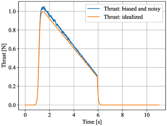
Figure 6. Example of regressive unitary thrust with bias and noise.

2.5.3. Ignition Dead Time

It corresponds to the dead time produced in the control signal due to electrical effects, and to the initial response of the igniter. This value is randomly selected in a uniform density between 0–2 s. It is important to note that the dead time is different and independent of the lag time ${\tau }_d$ from the Equation (5). To calculate the ignition dead time $t_d$ we use

$$t_d=\mathrm{Unif}(0,2)$$

(21)

This parameter could be decreased depending on the available technology, but decreasing the ignition response is a more difficult task because it depends on the atmospheric condition of the igniter.

3. Optimization Problem

The solution of the optimization problem (OP) of the control function is presented. Due to the behavior of the dynamics model, mass flow rate of the propellant, noise and dead time added in the engines, the problem is not linear. On the other hand, the optimization process is present to design a robust control system whose parameters are evaluated in stochastic scenarios. These stochastic analyses are tackled commonly with heuristic methods such as Genetic algorithm (GA) [30], and it is implemented in this work to find the optimal control parameters. As summary, GA is defined as follows by M. Jamshidi et al. [31]:

GA are optimization methods, which operate on a population of points, designated as individuals. Each individual of the population represents a possible solution of the OP. Individuals are evaluated depending upon their fitness. The fitness indicates how well an individual of the population solves the OP.

For the purposes of this project, the fitness indicator is called cost function. We will first define the elements that make up an individual and then, the cost function. The individual is a set of parameters that include the control gains, the maximum mass flow $\dot{m}$ and the action time $t_a$ of the engines. The following subsection presents the details of each set of elements.

3.1. GA Functionality

In order for the GA to recreate the natural evolutionary process and find an optimal solution, it is necessary to define the terminology involved in the general process. First, the first generation of population must be created, which is usually formed randomly according to the margins of the variables. This first generation is evaluated in the landing process by calculating a cost function that delivers an error value with respect to the target. Subsequently, each of the cost functions of the population’s individuals are compared to form a second generation. This process is divided into selection, to choose the best individuals called parents; crossover, to create new individuals between two parents; and mutation, to randomly affect a parameter within the individual ($\dot{m}$ for example) and prevent them from getting stuck. The full process is shown in Figure 7, accompanied by Equation (24) and the definition of the population set $\mathcal{P}$.

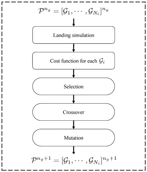
Figure 7. Representation of the evolutionary process of the GA, where the landing simulation is used to create a new generation of population $\mathcal{P}$.

For the selection process, 20% of the individuals with the lowest cost function are selected directly. The remaining 80% is selected using the roulette method. For the crossover. we use two types of operators alternately to accelerate the optimization: the one point crossover, and arithmetic crossover. The one point crossover cuts the individual of two parents randomly selected to create two children (the position of the cut is also chosen randomly). Arithmetic crossover assigns weights to both parents and then performs an arithmetic sum for each parameter within the individual. For this project, a weight of 0.3 and 0.7 was used to create two children, respectively. For the mutation process, each parameter within the individual is randomly assigned a probability of mutating from 0 to 1, if one of this is less than the probability of mutation, then that parameter mutates within the value ranges. To continue, the specific definitions of individual parameters and cost functions are introduced in the following sections.

3.2. Design of Control Function

The design of a control function that represents the ignition point $t_{ig,k}$ of each k-engine is explained. Its construction is based on a polynomial function such that whatever the polynomial is, it must contain the origin as the root and no zeros in the left half of the Cartesian plane formed by the variables y and v. The polynomial that satisfies the above requirements is defined as

$${\beta }_k^p={\alpha }_{k}y\left(t\right)+\sum _{j=1}^p{(-1)}^{j-1}{\left({\gamma }_k\right)}_{j}v{\left(t\right)}_j$$

(22)

where p is the polynomial degree, and ${\alpha }_k$ with ${\gamma }_k$ are the gains that will be optimized for each engine. For the purpose of this work, we select a simple expression that is a candidate to be the control function, which is a linear function with $p=1$ (the expression of $p=1$ is removed to simplify the general notation). Then, Equation (22) is defined as

$${\beta }_k\left(t\right)={\alpha }_{k}y\left(t\right)+{\gamma }_{k}v\left(t\right)$$

(23)

The control function ${\beta }_k\left(t\right)$ generates the following instructions: when ${\beta }_k\left(t\right)$ is greater than zero, the k-engine stay off; when ${\beta }_k\left(t\right)$ is less than zero, the k-engine begin the ignition as shown in the Figure 8. It is important to note that this function, being a straight line in the Cartesian plane, does not represent the real trajectory or velocity. This function only represents the ignition point at the instant $t_{ig,k}$, i.e., ${\beta }_k\left(t\right)\le 0$.

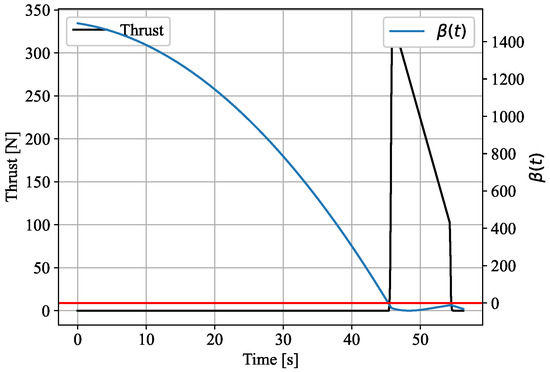
Figure 8. Example of activation of each engine. When the control function $\beta$ is less than zero, crossing the red line, the engine turns on at the instant $t_{ig,k}$ of the simulation. The ignition delay seen in the figure is due to the dead time of the propellant.

3.3. Individual Parameters

The parameters to be optimized are the control gains, the mass flow $\dot{m}$, and the action time $t_a$. To solve, we propose the following format for a GA individual ${\mathcal{G}}_i$:

$$\begin{array}{c}\hfill {\mathcal{G}}_i={\left[\dot{m},t_a,{\alpha }_{k=1},\cdots ,{\alpha }_{k=N_e},{\gamma }_{k=1},\cdots ,{\gamma }_{k=N_e}\right]}_i.\end{array}$$

(24)

where i represent the i-th individual of a generation $n_g$ of population ${\mathcal{P}}^{n_g}=[{\mathcal{G}}_1,\cdots ,{\mathcal{G}}_{N_i}]$, with $N_i$ the number of individuals in the population. The creation of each individual of the first generation is made randomly according to the Table 3.

Table 3. Creation of each gene of the first generation of individuals.

Genes	Random Method
$\dot{m}$	$\mathrm{Unif}({\dot{m}}_{min},{\dot{m}}_{max})$
$t_a$	$\mathrm{Unif}(0.0,{\left(t_a\right)}_{max})$
${\alpha }_k$	$\mathrm{Triang}(left={\left({\alpha }_k\right)}_{min},right={\left({\alpha }_k\right)}_{max},center)$
${\gamma }_k$	$\mathrm{Triang}(left={\left({\gamma }_k\right)}_{min},right={\left({\gamma }_k\right)}_{max},center)$

Here, $\mathrm{Triang}$ is a distribution function with triangular density. Then, Table 4 shows the simulation parameters that are necessary for estimating the variable ranges utilized in the random methods, which are presented in Table 5.

3.4. Individuals Cost Function

To minimize the boundary condition and the required propellant mass for each individual in the GA, we define two approaches to solve the optimization. These approaches differ in the cost functions that are defined as direct cost function (DCF), for the first approach; and average cost function (ACF) for the second. The DCF calculates the cost function based on a single trajectory without uncertainties, while the ACF considers a population of trajectories with the uncertainties shown in the Equations (17), (18) and (20). The results obtained with the first approach justify the use of a second approach, which is based on a robust design of the controller.

3.4.1. Direct Cost Function

The DCF is defined as

$$\begin{array}{cc}\hfill J=& R_a{\left(y\left(t_{land}\right)-y_{land}\right)}^2+R_b{\left(v\left(t_{land}\right)-v_{land}\right)}^2\hfill \\ \hfill & +R_c\left(\frac{t_{land}}{t_{free}}\right)\hfill \end{array}$$

(25)

where R is a gain term, and $t_{free}$ is the free fall time. This time is used to reduce the magnitude of the landing time $t_{land}$ with respect to altitude and velocity error, and it is obtained by solving the polynomial below.

$$\frac{g}{2}{t}_{free}^2+v_0{t}_{free}+y_0=0$$

(26)

3.4.2. Average Cost Function

The ACF is based on the performance of an individual evaluated on different cases that differ by the initial state of the trajectories and the condition of the specific impulse. These cases are evaluated with the parameters of the individuals of the GA. Then, the best individual must be chosen based on the ACF $\mathcal{J}$ that is calculated with the cost $J_j$ of each case j tested in the training process by the Equation (25). Now, we define $\mathcal{J}$ for each individual of the GA as follows.

$$\begin{array}{cc}\hfill \mathcal{J}=& b_1{\mu }_J\left(J_j\right)+b_2{\sigma }_J\left(J_j\right)\hfill \end{array}$$

(27)

Here ${\mu }_J\left(J_j\right)$ and ${\sigma }_J\left(J_j\right)$ is the mean and standard deviation, respectively, of all costs $J_j$ associated with a single individual. The mean is calculated as

$${\mu }_J=\frac{1}{N_{cases}}\sum _{j=1}^{N_{cases}}{J}_j,$$

(28)

and the standard deviation ${\sigma }_J$ is defined as

$${\sigma }_J=\sqrt{\frac{1}{N_{cases}}{\displaystyle \sum _{j=1}^{N_{cases}}}{(J_j-{\mu }_J)}^2}.$$

(29)

The parameters $b_1$ and $b_2$ are gains, and $N_{cases}$ is the number of cases mentioned before. The benefit of this feature is that the selection of the best individual is based on statistical parameters that show how close all cases are to the expected landing state.

4. Study Scenarios

4.1. First Approach: Controller Optimization without Trajectory Uncertainties

This subsection presents the optimization for an ideal scenario without uncertainties on the training. For this scenario, we solve the optimization problem with cost function present in the Equation (25), that is, a single trajectory. The full process of optimization for this case is shown in Figure 9. The solutions obtained by the OC and the $N_e$ engines are then evaluated on an uncertain scenario. Each number of engines has a particular solution and is independent of another, so it is evaluated independently. These evaluations show the landing point for all trajectories and are used to form a velocity and altitude distribution. Subsequently, this information is used to obtain the mean and the standard deviation of the landing state for an arrangement configuration of the different numbers of engines.

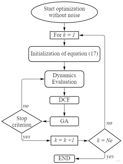
Figure 9. First approach: Optimization for scenarios without uncertainties in the training process.

4.2. Second Approach: Controller Optimization with Trajectory Uncertainties

As a counterpart to the previous subsection, in this scenario we use the information corresponding to the uncertainties to improve the landing of the model. Therefore, we optimize based on the recursion of the training using different initial conditions of the states for each number of engines and generation of the GA.

The optimization process begins by iterating from an array of engines from $k=1,\cdots ,N_e$, and with an initial population of candidate solutions in the GA. In each generation of the GA, we evaluate for different $N_e$. Then, the number of engines is fixed to generate $N_{case}$ of initial states defined by Equations (17), (18) and (21). Each of these initial states create a j-th trajectory with $j=1,\cdots ,N_{case}$. These cases are then evaluated in the dynamic model passing for all the individuals of the generation. In the dynamic model, the continuous noise of the specific impulse is added at each time step of the simulation. When the simulation ends, the cost of each trajectory is calculated separately according to Equation (25) and stored in a vector that regroups the costs of all the cases (trajectories). When all cases have been simulated, the ACF is calculated to execute the selection, crossing, and mutation process of the GA. Once some criteria for stopping the GA have been satisfied, the number k of engines in the arraignment is increased, and the same process mentioned above is carried out again until $N_e$. The full process is shown in Figure 10.

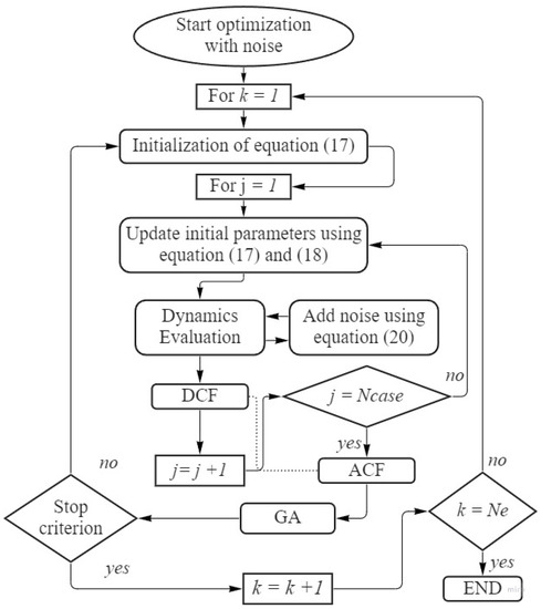
Figure 10. Second approach: Optimization for scenarios with uncertainties in the training process.

5. Simulation and Results

Based on the case studies, the simulations are separated into two evaluation scenarios using the Monte Carlo method: one that evaluates the first approach, and a second that evaluates the trajectories with the second approach. As both cases must be evaluated, we regroup the simulation data in the Table 4, which is also used in the optimization of the scenario with uncertainties. The altitude and velocity states are selected according to the final stage of soft-landing process, such as mentioned by [10,13,15]. The optimization parameters are shown in Table 5, where the limits of the mass flows of each individual are calculated as follows:

$${\dot{m}}_{min}=\frac{\left|g\right|m_0}{v_{e}k},{\dot{m}}_{max}=\frac{2{\dot{m}}_{*}}{k},k=1,\cdots ,N_e$$

(30)

where ${\dot{m}}_{*}$ is the theoretical optimal mass flow obtained from Pontryagin’s principle for a constant thrust and action time [11,12]. For simplicity, the action time used in ${\dot{m}}_{*}$ is equal to the mean between the $min\left(t_{a,k}\right)$ and $max\left(t_{a,k}\right)$, which is equal to $10.5$ s. As expressed in the Equation (30), the mass flows must be updated according to the number k of engines in the array.

Table 4. Simulation parameters.

Parameters	Value
$y_0$	2000 m
$v_0$	0 m/s
${\sigma }_{alt}$	50 m
${\sigma }_{vel}$	5 m/s
$I_{sp}$	300 s
${\sigma }_{bias}$	10.83 s (10% at $3\sigma$)
${\sigma }_{noise}$	3.25 s (3% at $3\sigma$)
$m_0$	24 kg
g Acceleration of the moon	1.67 [m/s2]
$\Delta t$ of simulation	0.1 s
Numerical method	Runge-Kutta 4th Order
${\tau }_d$	0.2 s
${\tau }_l$	0.5 s

Table 4. Simulation parameters.

Parameters	Value
$y_0$	2000 m
$v_0$	0 m/s
${\sigma }_{alt}$	50 m
${\sigma }_{vel}$	5 m/s
$I_{sp}$	300 s
${\sigma }_{bias}$	10.83 s (10% at $3\sigma$)
${\sigma }_{noise}$	3.25 s (3% at $3\sigma$)
$m_0$	24 kg
g Acceleration of the moon	1.67 [m/s2]
$\Delta t$ of simulation	0.1 s
Numerical method	Runge-Kutta 4th Order
${\tau }_d$	0.2 s
${\tau }_l$	0.5 s

Table 5. Optimization parameters.

Parameters	Value
$N_e$	10
$N_{case}$	30 in trained
$R_a,R_b,R_c$	$0.1,1.0,10.0$
$b_1,b_2$	1.0, 1.0
${\alpha }_k$	$\in [0.0,1.0]$
${\gamma }_k$	$\in [0.0,{\gamma }_{max}]$
$t_{a,k}$	$\in [1.0,20.0]$ s
$\dot{m}$	$\in [{\dot{m}}_{min},{\dot{m}}_{max}]$
Probability of mutation	0.25
Number of individuals	40
Number of generations	300
$center$	0.7

Table 5. Optimization parameters.

Parameters	Value
$N_e$	10
$N_{case}$	30 in trained
$R_a,R_b,R_c$	$0.1,1.0,10.0$
$b_1,b_2$	1.0, 1.0
${\alpha }_k$	$\in [0.0,1.0]$
${\gamma }_k$	$\in [0.0,{\gamma }_{max}]$
$t_{a,k}$	$\in [1.0,20.0]$ s
$\dot{m}$	$\in [{\dot{m}}_{min},{\dot{m}}_{max}]$
Probability of mutation	0.25
Number of individuals	40
Number of generations	300
$center$	0.7

The limits of the ${\alpha }_k$ and ${\gamma }_k$ control parameters are selected based on the dynamic model and the linear function defined in the plane. The limits of ${\alpha }_k$ were chosen between 0 and 1 to normalize one of the parameters of the linear function. On the other hand, for any speed and altitude value, the control function must cut the height axis between the initial speed $y_0$ and the final speed $y_{land}$. To understand the relationship that exists between the control variables, it is useful to express the Equation (23) as,

$$y\left(t\right)=-\frac{{\gamma }_k}{{\alpha }_k}v\left(t\right)$$

(31)

where we can see that if ${\alpha }_k$ is small, the slope tends to infinity. To counter this, the value of ${\gamma }_k$ must also tend to zero. Then, the minimum value of ${\gamma }_k$ is zero.

The worst-case scenario is when ${\alpha }_k$ stagnates at its maximum value, where the slope only depends on ${\gamma }_k$. If this value is not high enough, the maximum slope will not be able to reach optimal ranges. However, if it is too high, it could take a long time for GA to find an optimal solution. To satisfy these two points, we define that the control line must pass through the point that contains the initial altitude and the final velocity in free fall. In this way, the maximum value of ${\gamma }_k$ is defined as follows.

$${\gamma }_{max}=\frac{y_0}{\sqrt{v_0^2+2\left|g\right|y_0}}$$

(32)

This analysis is performed with a simulator developed in Python, which is available in the Space Exploration and Planetary Laboratory (SPEL) repository (https://github.com/spel-uchile/SolidPropellantforLanding (accessed on 20 September 2022)).

5.1. Optimization and Evaluation of First Approach

In this section, the best result obtained with the DCF approach in the scenario of the Section 4.1 is present. These optimal parameters are evaluated in a scenario with all the mentioned uncertainties. In this evaluation, it is possible to differentiate the point with the lowest impact velocity, resulting in the control and optimization parameters shown in Table 6 and Table 7 for Regressive PGCS.

Table 6. Design parameters of the best result obtained from the optimization scenario without uncertainties.

Parameters	Value
PGCS	Regressive
$N_e$	9
$\dot{m}$	14.15 × 10${}^{-3}$ kg/s
$t_a$	$15.75$ s
$v_{land}$	$-5.87$ m/s
Std Dev. of $v_{land}$	$2.49$ m/s
Mass used	$1.51$ kg

Table 7. Control parameters from the best result obtained in the scenario without optimization uncertainties. The SPEs array has $N_e=9$ and Regressive PGCS.

k	${\mathsf{\alpha }}_{\mathit{k}}$	γk
1	0.511	3.632
2	0.992	4.393
3	0.300	10.071
4	0.755	19.199
5	0.531	20.431
6	0.795	11.292
7	0.560	17.099
8	0.323	8.667
9	0.729	16.382

The behavior of the altitude and the velocity of the lander are shown in Figure 11, while the distribution is shown in Figure 12. Here, it is possible to see that the impact velocity is $-5.87$ m/s with a standard deviation of $2.49$ m/s. Additionally, the green and red circles in Figure 11 represent the ignition time and the shutdown time of each engine, respectively.

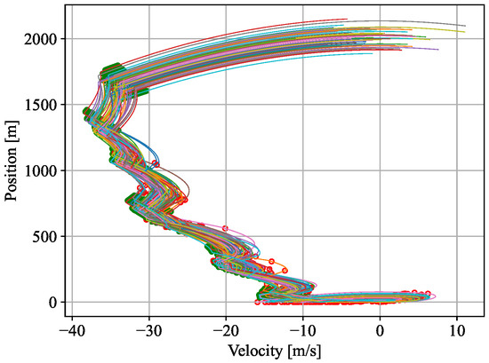
Figure 11. Behavior of altitude and velocity in the evaluation of the best individual $\mathcal{G}$ obtained from the optimization without uncertainties in training. The SPEs array has $N_e=9$ and Regressive PGCS. Color map is used to differentiate different random trajectories.

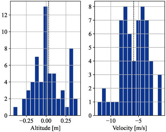
Figure 12. Distribution of altitude and velocity landing in the evaluation of the best result obtained from the optimization without uncertainties in training. The SPEs array has $N_e=9$ and Regressive PGCS. The vertical axis shows the frequency of the values.

In Figure 13, we present the performance for different numbers of engines and PGCS. Although the result shows a certain pattern to improve the landing process, it has an undefined pattern for a certain number of engines and type of PGCS. On the other hand, the standard deviation of the results does not decrease as a function of the number of engines. This randomness is one of the main reasons why it is necessary to use the method presented in Section 4.2. These results are presented in the next subsection.

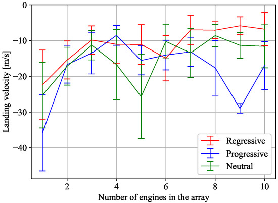
Figure 13. First approach: performance comparison for an array between 1 and 10 configuration engines, and for the three types of PGCS: Regressive, Neutral and Progressive.

5.2. Optimization and Evaluation of Second Approach

In this scenario, all the information corresponding to the uncertainties is used to optimize the landing. Such optimization shows poor performance if performed with a single engine, but it improves as the number of engines in the array increases. This not only decreases the landing velocity, but also decreases the standard deviation in the evaluation. The evaluation of the optimization result shows that the best configuration is given for a number of engines equal to $N_e=10$ and a Regressive PGCS. The altitude and velocity variables of the best result are shown in Figure 14, while the distribution of the landing parameters is shown in Figure 15. The optimization obtained is grouped in Table 8 for the arrangement of engines, where for $N_e=10$ shown a landing velocity of $-2.97$ m/s and standard deviation of $0.993$ m/s. Additionally, the control parameters are in Table 9.

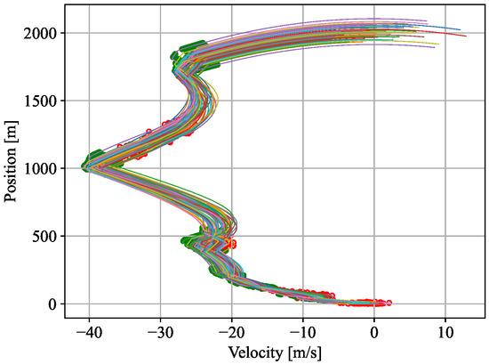
Figure 14. Behavior of altitude and velocity in the evaluation of the best $\mathcal{G}$ obtained from the optimization with uncertainties and $N_e=10$. Color map is used to differentiate different random trajectories.

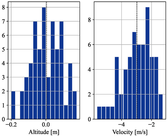
Figure 15. Distribution of altitude and velocity landing in the evaluation of the best result obtained from the optimization with uncertainties and $N_e=10$. The vertical axis shows the frequency of the values.

Table 8. Design parameters of the best result obtained from the optimization scenario with uncertainties.

Parameters	Value
PGCS	Regressive
$N_e$	10
$\dot{m}$	10.16 × 10${}^{-3}$ kg/s
$t_a$	$20.0$ s
$v_{land}$	$-2.97$ m/s
Std Dev. of $v_{land}$	$0.99$ m/s
Mass used	$1.35$ kg

Table 9. Control parameters from the best result obtained in the scenario with optimization uncertainties.

k	${\mathsf{\alpha }}_{\mathit{k}}$	γk
1	0.639	12.111
2	0.138	11.165
3	0.862	4.742
4	0.551	12.844
5	0.999	11.465
6	0.091	6.036
7	0.768	22.285
8	0.608	5.219
9	0.624	17.851
10	0.867	24.439

As supported by Figure 16, we see that the pattern of the performance curves shows asymptotic behavior. This pattern indicates a relationship between the increase in the number of engines and the increase in landing performance. Therefore, $N_e=10$ is a local optimum based on the limits summed up in this work.

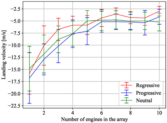
Figure 16. Second approach: Performance comparison for an array between 1 and 10 configuration engines, and for the three types of PGCS: Regressive, Neutral and Progressive.

6. Discussion

The optimization carried out with the first approach of Figure 9 generated worse scenarios in the evaluation with landing velocity over the $5.87$ m/s. Even so, the regressive PGCS simulation in Figure 13 shows better performance than the other types of PGCS. In this scenario, it is possible to see that the ignition points of the k-engines of the simulations (the group of green circles in Figure 11) do not belong exactly to the control function line. This phenomenon is caused by the dead time $t_d$ and it is observed when $t_d>0$. In this way, while there is uncertainty about the dead time, all engines start their ignitions below the control function. By not considering this in the classic design of the controller, we can see that the impact velocity distribution of the evaluation has values greater than 10 m/s (see Figure 12). Using the approach presented in Figure 9, it is not possible to see a clear pattern in the performance of the landing system based on an arrangement of SPEs.

With the second approach summarized in Figure 10, we can see an improvement in the performance of the propulsion system. Figure 16 shows a performance curve that improves asymptotically with increasing the number of engines. This not only decreases the impact velocity to $-2.97,-4.13,-4.77$ m/s for Regressive, Progressive, and Neutral, respectively, but also decreases the standard deviation to $0.99,1.55,1.87$ m/s. This is reflected in the impact velocity distribution for the 60 cases evaluated in simulation, which are shown in Figure 15. Additionally, to demonstrate the asymptotic behavior of the performance, an auxiliary simulation is performed with $N_e=16$. Figure 17 shows the behavior of the altitude and velocity, meanwhile Figure 18 shows the distribution. From this distribution, it can be seen that the mean landing speed is $-2.04$ m/s and the standard deviation is $0.48$ m/s. Although these values are above the landing speed of $-1.7$ m/s of the Chang’E 5 module [17], they are well below what was the landing of the MPF with $-12.5$ m/s, and the CubeSat OMOTENASHI with $-30$ m/s. Finally, the total mass used by the propellant in the soft-landing stage is 1.35 kg, which corresponds to 5.62% of the 12U CubeSat mass.

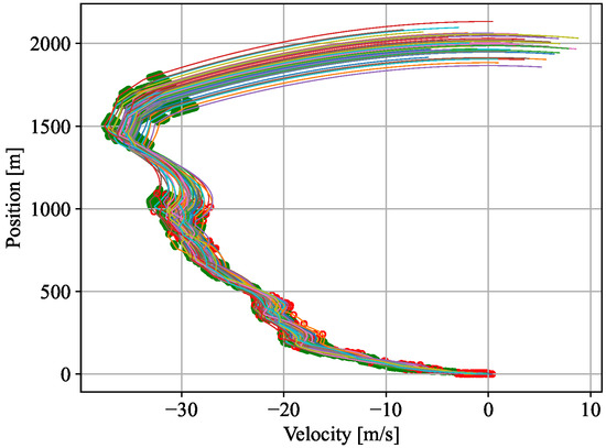
Figure 17. Behavior of altitude and velocity in the evaluation of the best $\mathcal{G}$ obtained from the optimization with uncertainties and $N_e=16$. Color map is used to differentiate different random trajectories.

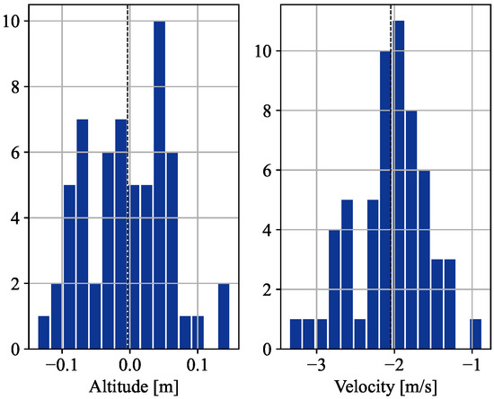
Figure 18. Distribution of altitude and velocity landing in the evaluation of the best result obtained from the optimization with uncertainties and $N_e=16$. The vertical axis shows the frequency of the values.

With respect to the dead time, the evaluation of the second approach shows that the control design is robust to the ignition dead times. This improvement is more evident in a regressive PGCS, which can be designed as a star type with ${\theta }_d<{\theta }_{neutral}$ as shown by the Equation (4). Lastly, a star-type burn configuration can work with a thinner-walled engine to withstand the temperatures and pressures of the combustion chamber. This helps to decrease the weight of the engines, as mentioned in Table 1. However, this configuration has a small action time $t_a$ compared to the results in the Table 6 and Table 8. Therefore, it is recommended as future work to perform an optimization with limits on the engine design. For now, the focus of this work is to present landing effectiveness and find the type of burn with the best performance.

7. Conclusions

In this paper, a methodology to solve the soft-landing problem with an array of solid propellant engines (SPEs) is present. This study was performed by using a 1-dimensional dynamic model and for different numbers of engines in the array, where each one is controlled independently by a linear control function. This linear function is designed with two gains, ${\alpha }_k$ and ${\gamma }_k$ for each engine, which are optimized by GA and using two different approaches. Consequently, the optimization based on the second approach and robust design (Section 4.2) presents better results in the evaluation simulations that considered the uncertainties of the variables. The results show that the SPEs array generates an asymptotic increase in performance as the number of engines increases, which also helped to decrease the standard deviation of the impact velocity distribution. For a range of $N_e\in [0,10]$, the lowest impact velocity is $-2.97$ m/s with a standard deviation of $0.99$ m/s for $N_e=10$. An auxiliary study is presented for $N_e=16$ to demonstrate the asymptotic behavior, showing that the landing speed is $-2.04$ m/s with a standard deviation of $0.48$ m/s. These results show that the regressive propellant grain cross-sections (PGCS) allow landings with lower impact velocities than those obtained with progressive and neutral PGCS. A regressive PGCS solid propellant engine can be designed with a star-type cross-section with ${\theta }_d<{\theta }_{neutral}$, as shown by the Equation (4). On the other hand, this approach is independent of the thrust profile modeled in this work, and it can be replaced by measured thrust data. Finally, the algorithms used to model, simulate, and optimize the control scenarios were uploaded to a GitHub repository with a free license (https://github.com/spel-uchile/SolidPropellantforLanding (accessed on 20 September 2022)).

References

- Siddiqi, A.A. Beyond Earth: A Chronicle of Deep Space Exploration, 1958–2016, 2nd ed.; Number 2018-4041 in NASA SP; National Aeronautics and Space Administration, Office of Communications, NASA History Division: Washington, DC, USA, 2018.
- Kajon, D.; Masson, F.; Wagner, T.; Welberg, D. Development of an Attitude Control and Propellant Settling System for the aA5ME Upper Stage. In Proceedings of the Space Propulsion Conference, Cologne, Germany, 19–22 May 2014; p. 9. [Google Scholar]
- Morrisey, D.C. Historical perspective—Viking Mars Lander propulsion. J. Propuls. Power 1992, 8, 320–331. [Google Scholar] [CrossRef]
- Soffen, G.A.; Snyder, C.W. The First Viking Mission to Mars. Science 1976, 193, 759–766. [Google Scholar] [CrossRef] [PubMed]
- Maggi, F.; Bandera, A.; Galfetti, L.; De Luca, L.T.; Jackson, T.L. Efficient solid rocket propulsion for access to space. Acta Astronaut. 2010, 66, 1563–1573. [Google Scholar] [CrossRef]
- Chavers, D.G. NASA Lander Technologies Project Status. In AIAA SPACE 2016; American Institute of Aeronautics and Astronautics: Long Beach, CA, USA, 2016. [Google Scholar] [CrossRef]
- Spear, A.J. Low cost approach to Mars Pathfinder and small landers. Acta Astronaut. 1995, 35, 345–354. [Google Scholar] [CrossRef]
- Kalita, H.; Thangavelautham, J. Lunar CubeSat Lander to Explore Mare Tranquilitatis pit. In AIAA Scitech 2020 Forum; American Institute of Aeronautics and Astronautics: Orlando, FL, USA, 2020. [Google Scholar] [CrossRef]
- Grimm, C.D.; Witte, L.; Schröder, S.; Wickhusen, K. Size matters-The shell lander concept for exploring medium-size airless bodies. Acta Astronaut. 2020, 173, 91–110. [Google Scholar] [CrossRef]
- Hashimoto, T.; Yamada, T.; Otsuki, M.; Yoshimitsu, T.; Tomiki, A.; Torii, W.; Toyota, H.; Kikuchi, J.; Morishita, N.; Kobayashi, Y.; et al. Nano Semihard Moon Lander: OMOTENASHI. IEEE Aerosp. Electron. Syst. Mag. 2019, 34, 20–30. [Google Scholar] [CrossRef]
- Meditch, J. On the problem of optimal thrust programming for a lunar soft landing. IEEE Trans. Autom. Control 1964, 9, 477–484. [Google Scholar] [CrossRef]
- Fleming, W.; Rishel, R. Deterministic and Stochastic Optimal Control; Springer: New York, NY, USA, 1975. [Google Scholar] [CrossRef]
- Acikmese, B.; Ploen, S.R. Convex Programming Approach to Powered Descent Guidance for Mars Landing. J. Guid. Control Dyn. 2007, 30, 1353–1366. [Google Scholar] [CrossRef]
- Xu, B.; Sun, J.; Li, S.; Cao, T. Finite time sliding sector control for spacecraft atmospheric entry guidance. Acta Astronaut. 2018, 163, 108–113. [Google Scholar] [CrossRef]
- Zhang, Y.; Guo, Y.; Ma, G.; Wie, B. Fixed-time pinpoint mars landing using two sliding-surface autonomous guidance. Acta Astronaut. 2019, 159, 547–563. [Google Scholar] [CrossRef]
- Liu, X.L.; Duan, G.R.; Teo, K.L. Optimal soft landing control for moon lander. Automatica 2008, 44, 1097–1103. [Google Scholar] [CrossRef]
- Zhang, H.; Li, J.; Wang, Z.; Guan, Y. Guidance Navigation and Control for Chang’E-5 Powered Descent. Space Sci. Technol. 2021, 2021, 1–15. [Google Scholar] [CrossRef]
- Rom, H. Thrust Control of Hydrazine Rocket Motors by Means of Pulse Width Modulation. Acta Astronaut. 1992, 26, 313–316. [Google Scholar] [CrossRef]
- Mishra, D.P. Fundamentals of Rocket Propulsion; CRC Press: Boca Raton, FL, USA, 2017. [Google Scholar] [CrossRef]
- Park, S.; Choi, S. A Study on the Characteristics of Solid Propellant Using a Defoamer. Propellants Explos. Pyrotech. 2020, 45, 486–492. [Google Scholar] [CrossRef]
- Klumpp, A.R. Apollo lunar descent guidance. Automatica 1974, 10, 133–146. [Google Scholar] [CrossRef]
- Marrison, C.; Stengel, R. Robust control system design using random search and genetic algorithms. IEEE Trans. Autom. Control 1997, 42, 835–839. [Google Scholar] [CrossRef]
- Herreros, A.; Baeyens, E.; Perán, J.R. MRCD: A genetic algorithm for multiobjective robust control design. Eng. Appl. Artif. Intell. 2002, 15, 285–301. [Google Scholar] [CrossRef]
- Gao, Y.; Wang, J.; Gao, S.; Cheng, Y. An Integrated Robust Design and Robust Control Strategy Using the Genetic Algorithm. IEEE Trans. Ind. Inform. 2021, 17, 8378–8386. [Google Scholar] [CrossRef]
- Sekaj, I. Genetic Algorithm Based Controller Design. IFAC Proc. Vol. 2003, 36, 125–128. [Google Scholar] [CrossRef]
- Jamanca Lino, G. Space Resources Engineering: Ilmenite Deposits for Oxygen Production on the Moon. Am. J. Min. Metall. 2021, 6, 6–11. [Google Scholar] [CrossRef]
- Moore, J.; Calvert, D.; Frady, G.; Chavers, G.; Hull, P.; Lowery, E.; Farmer, J.; Trinh, H.; Rojdev, K.; Piatek, I.; et al. Resource Prospector Lander: Architecture and trade studies. In Proceedings of the 2015 IEEE Aerospace Conference, Big Sky, MT, USA, 7–14 March 2015. [Google Scholar]
- Sutton, G.P. Rocket Propulsion Elements, 9th ed.; John Wiley & Sons (US): Hoboken, NJ, USA, 2017; Google-Books-ID: GS9gswEACAAJ. [Google Scholar]
- Stein, S.D. Benefits of the Star Grain Configuration for a Sounding Rocket; United States Air Force Academy: Colorado Springs, CO, USA, 2008; p. 11. [Google Scholar]
- Rao, A. A Survey of Numerical Methods for Optimal Control. Adv. Astronaut. Sci. 2010, 135, 1–32. [Google Scholar]
- Jamshidi, M.; Krohling, R.A.; Coelho, L.d.S.; Fleming, P.J. Robust Control Systems with Genetic Algorithms; CRC Press: Boca Raton, FL, USA, 2017. [Google Scholar] [CrossRef]
Publisher’s Note: MDPI stays neutral with regard to jurisdictional claims in published maps and institutional affiliations. |
© 2022 by the authors. Licensee MDPI, Basel, Switzerland. This article is an open access article distributed under the terms and conditions of the Creative Commons Attribution (CC BY) license (https://creativecommons.org/licenses/by/4.0/).