An Inversion Method Based on Inherent Similarity between Signals for Retrieving Source Mechanisms of Cracks

Abstract
:1. Introduction
2. Formulas
2.1. Review of Standard Moment Tensor Inversion
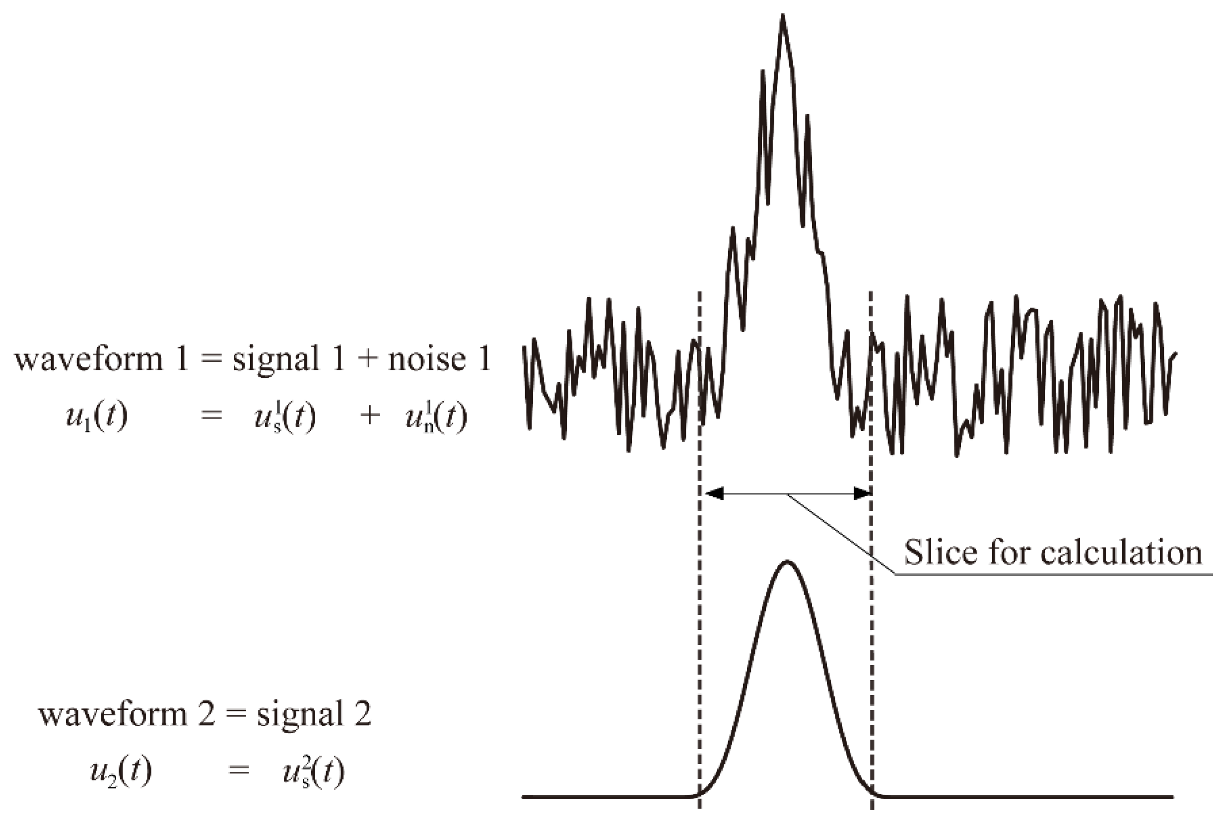
2.2. Correlation Function of Raw Waveform
2.3. Mechanism of New Correlation Function for De-Noising
3. Synthetic Tests
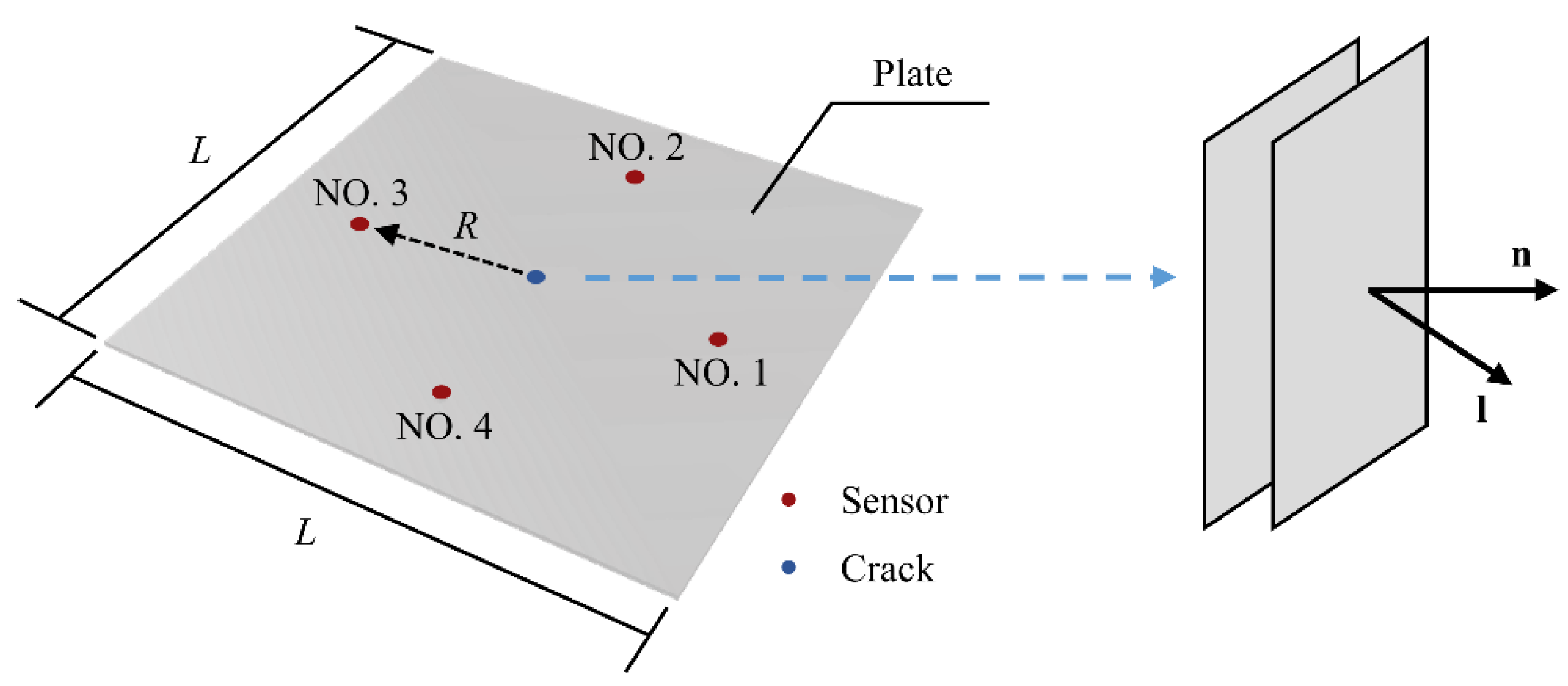
3.1. Model Parameters
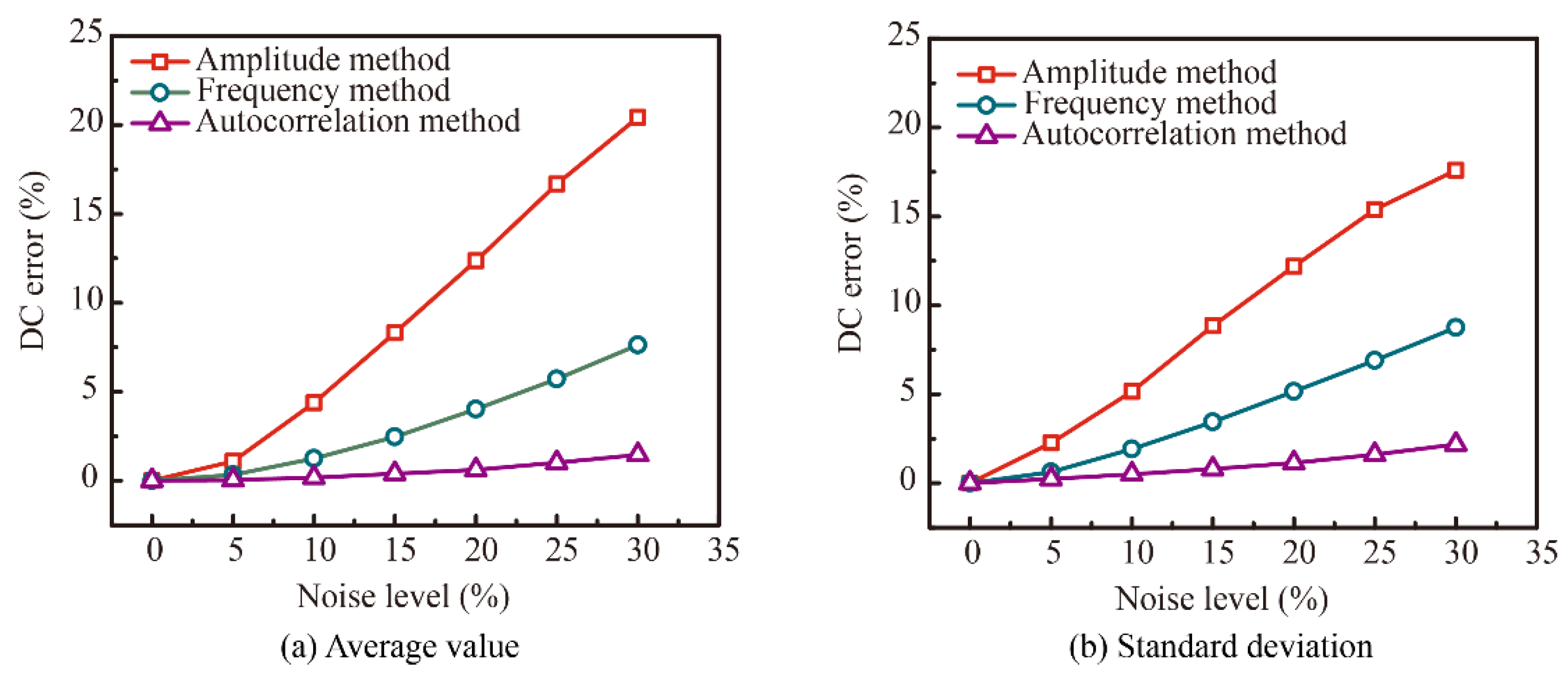
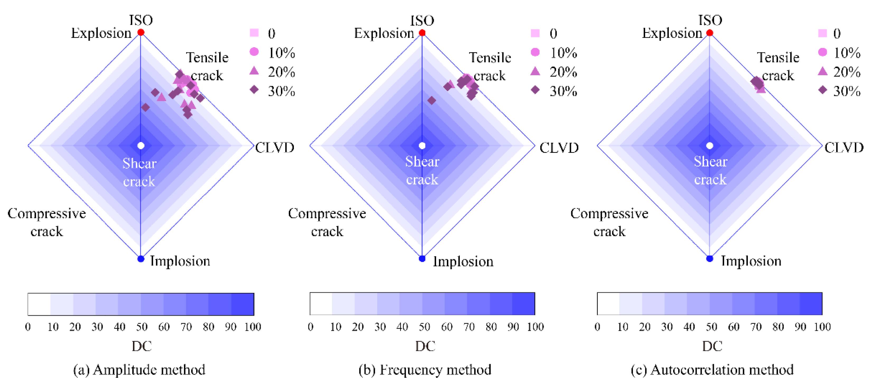
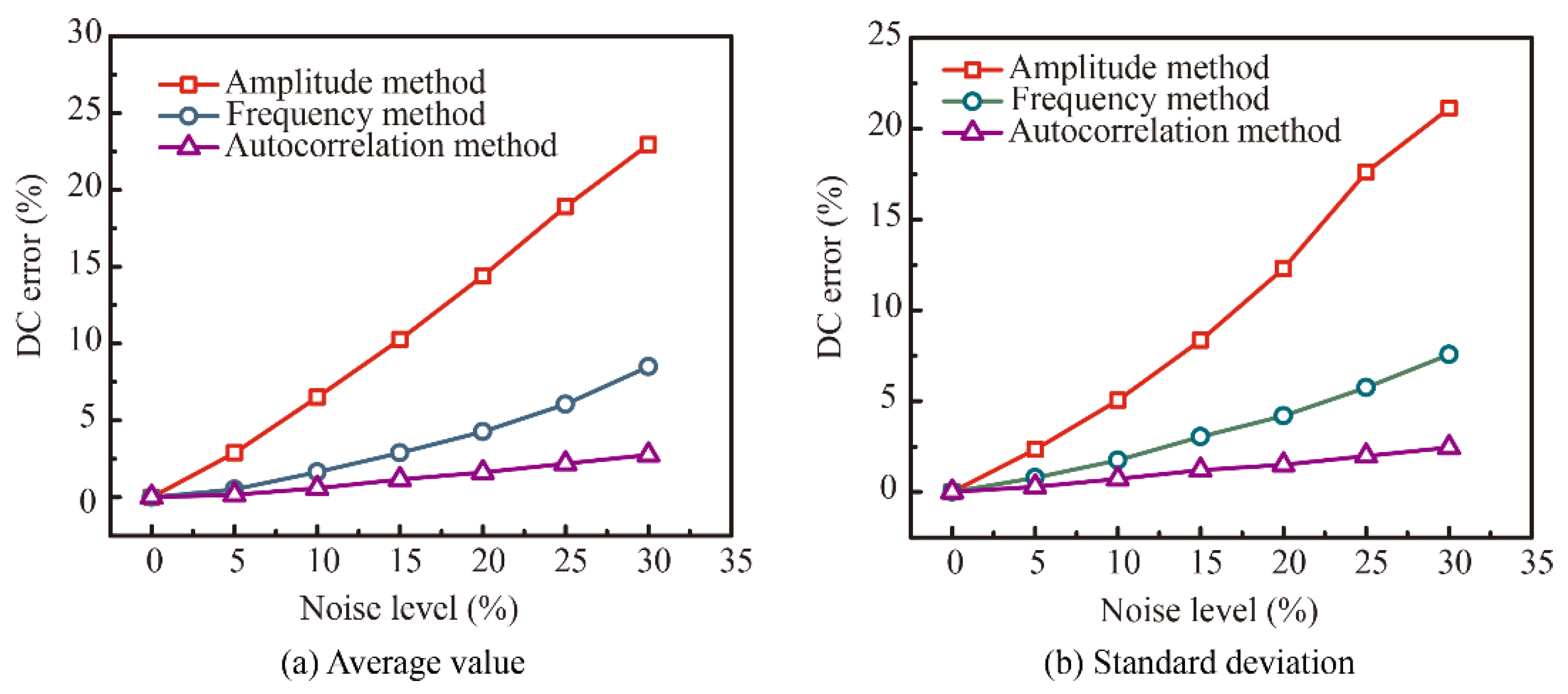
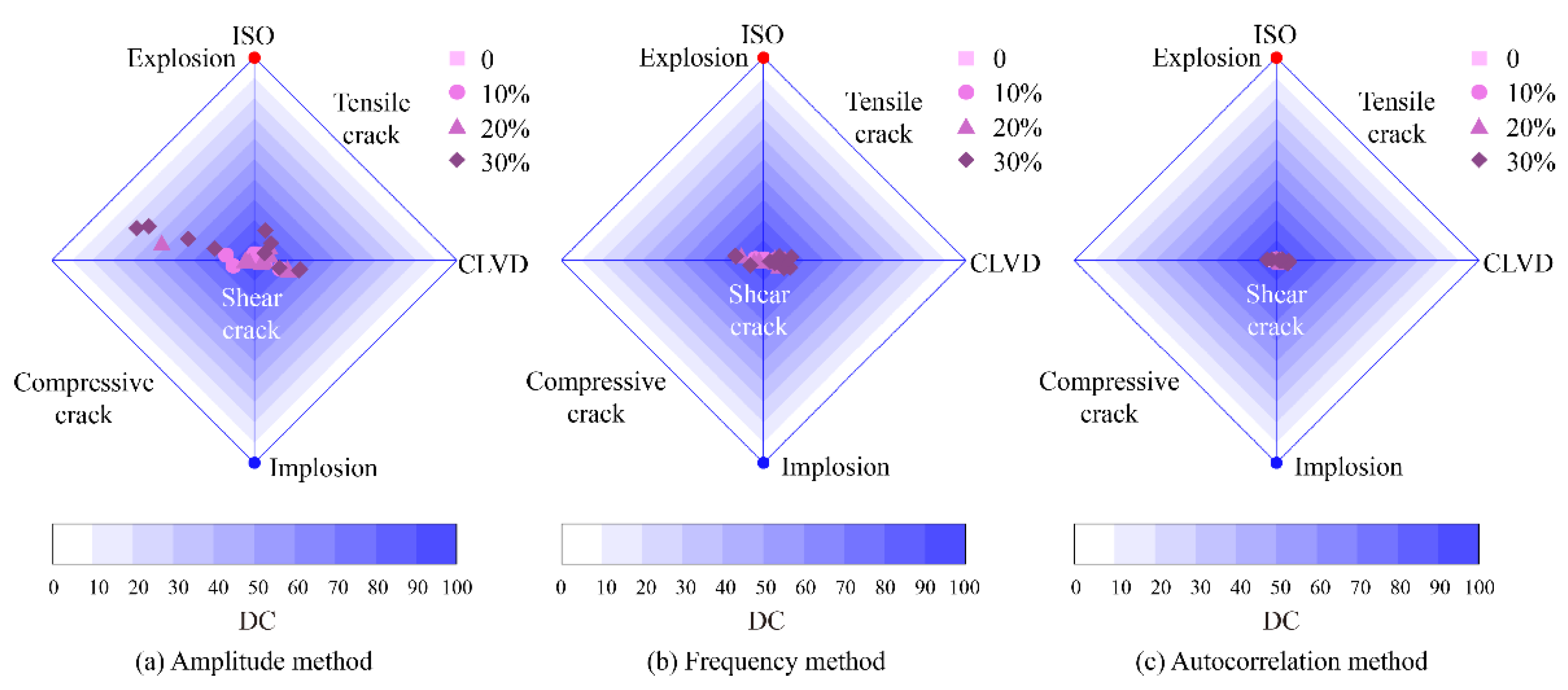
3.2. Inversion Results
4. Discussion
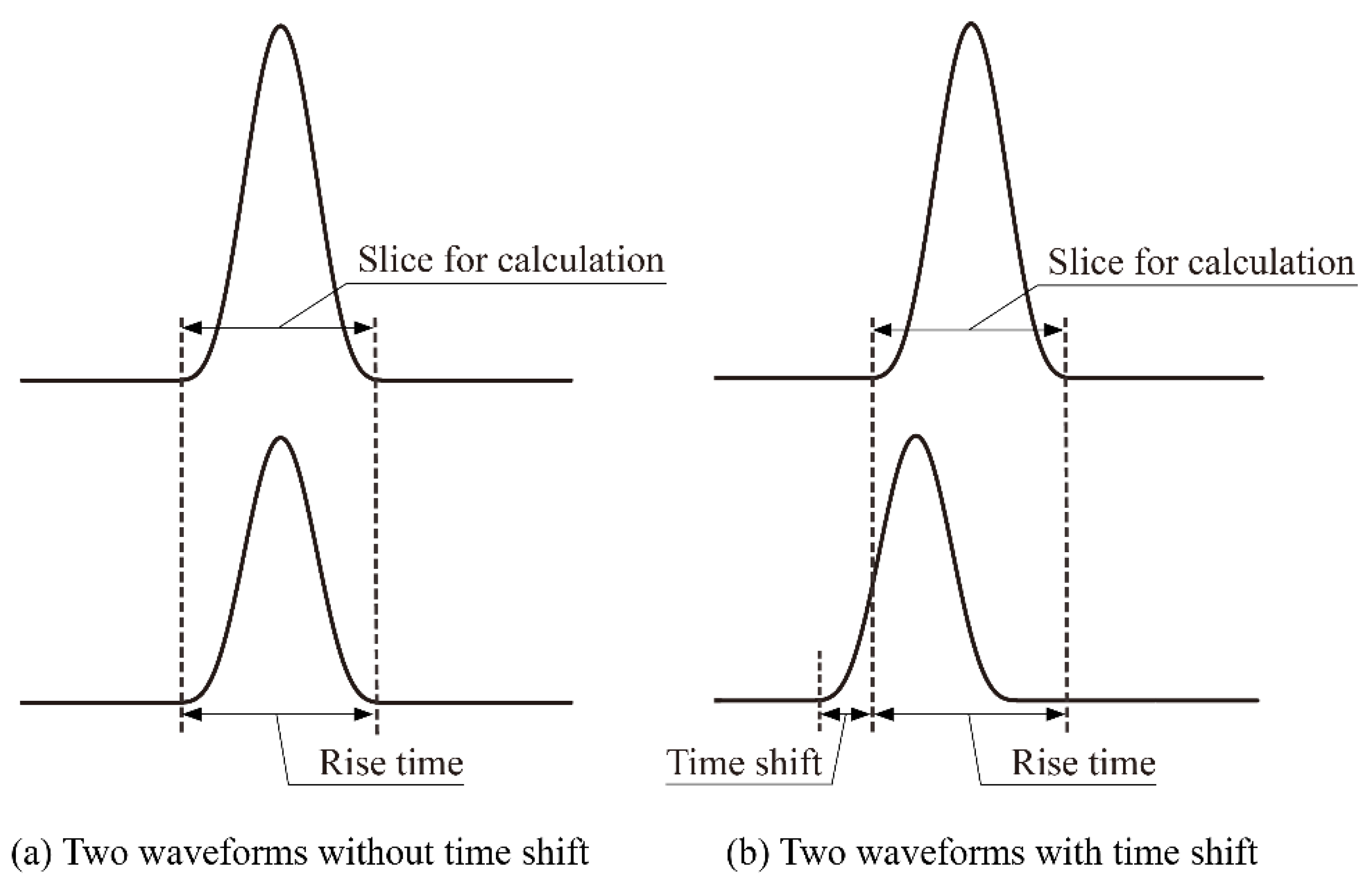
4.1. Time Shift
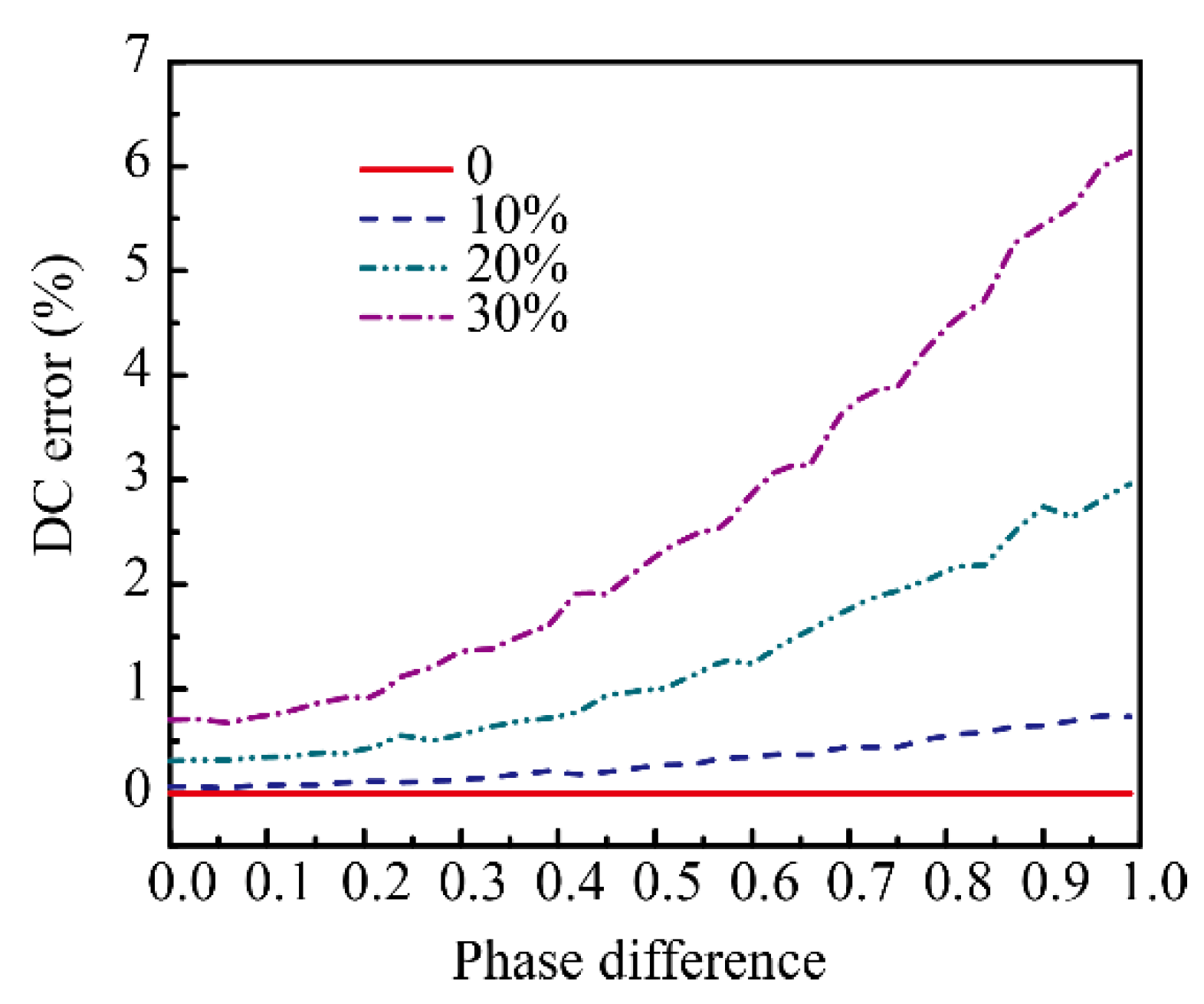
4.2. Spectrum Difference
5. Conclusions
Author Contributions
Funding
Conflicts of Interest
References
- Rokhlin, S.I.; Zoofan, B.; Kim, J.-Y. Microradiographic characterization of pitting corrosion damage and fatigue life. In Review of Progress in Quantitative Nondestructive Evaluation; Thompson, D.O., Chimenti, D.E., Eds.; Springer: Boston, MA, USA, 1999; Volume 18A–18B, pp. 1795–1804. [Google Scholar]
- Bieber, J.A.; Tai, C.-C.; Moulder, J.C. Quantitative assessment of corrosion in aircraft structures using scanning pulsed eddy current. In Review of Progress in Quantitative Nondestructive Evaluation; Thompson, D.O., Chimenti, D.E., Eds.; Springer: Boston, MA, USA, 1998; Volume 17A, pp. 315–322. [Google Scholar]
- Yan, Z.; Xiao, H.; Nagy, P.B. Ultrasonic detection of fatigue cracks by thermo-optical modulation. In Review of Progress in Quantitative Nondestructive Evaluation; Thompson, D.O., Chimenti, D.E., Eds.; Springer: Boston, MA, USA, 1999; Volume 18A–18B, pp. 1779–1786. [Google Scholar]
- Grondel, S.; Delebarre, C.; Assaad, J.; Dupuis, J.-P.; Reithler, L. Fatigue crack monitoring of riveted aluminium strap joints by Lamb wave analysis and acoustic emission measurement techniques. NDT E Int. 2002, 35, 137–146. [Google Scholar] [CrossRef]
- Joosse, P.A.; Blanch, M.J.; Dutton, A.G.; Kouroussis, D.A.; Philippidis, T.P.; Vionis, P.S. Acoustic Emission Monitoring of Small Wind Turbine Blades. J. Sol. Energy Eng. 2002, 124, 446–454. [Google Scholar] [CrossRef]
- Yu, J.; Ziehl, P.; Zárate, B.; Caicedo, J. Prediction of fatigue crack growth in steel bridge components using acoustic emission. J. Constr. Steel Res. 2011, 67, 1254–1260. [Google Scholar] [CrossRef]
- Martin, C.A.; Van Way, C.B.; Lockyer, A.J.; Kudva, J.N.; Ziola, S.M. Acoustic emission testing on an F/A-18 E/F titanium bulkhead. In Smart Structures and Materials 1995: Smart Sensing, Processing, and Instrumentation; SPIE: Bellingham, WA, USA, 1995. [Google Scholar]
- Haile, M.A.; Bordick, N.E.; Riddick, J.C. Distributed acoustic emission sensing for large complex air structures. Struct. Health Monit. 2017, 17, 624–634. [Google Scholar] [CrossRef]
- Han, C.; Liu, T.; Jin, Y.; Yang, G. Acoustic Emission Intelligent Identification for Initial Damage of the Engine based on Single Sensor. Mech. Syst. Signal Process. 2022, 169, 108789. [Google Scholar] [CrossRef]
- Schijve, J. Fatigue of Structures and Materials; Springer: Dordrecht, The Netherlands, 2001. [Google Scholar]
- Pook, L.; Greenan, A. Fatigue crack-growth characteristics of two magnesium alloys. Eng. Fract. Mech. 1973, 5, 935–946. [Google Scholar] [CrossRef]
- Daiuto, R.; Hillberry, B. The Effect of Thickness on Fatigue Crack Propagation in 7475-T731 Aluminum Alloy Sheet; Purdue University: West Lafayette, IN, USA, 1984. [Google Scholar]
- Zuidema, J.; Blaauw, H. The effect of shearlips on fatigue crack growths in A1-2024 sheet material. In Proceedings of the Third International Conference on Fatigue and Fatigue Thresholds, University of Virginia, Charlottesville, VA, USA, 28 June–3 July 1987. [Google Scholar]
- Burridge, R.; Knopoff, L. Body force equivalents for seismic dislocations. Bull. Seism. Soc. Am. 1964, 54, 1875–1888. [Google Scholar] [CrossRef]
- Aki, K.; Richards, P.G. Quantitative Seismology; University Science Books: Sausalito, CA, USA, 2002. [Google Scholar]
- Vavryčuk, V.; Bohnhoff, M.; Jechumtálová, Z.; Kolář, P.; Šílený, J. Non-double-couple mechanisms of microearthquakes induced during the 2000 injection experiment at the KTB site, Germany: A result of tensile faulting or anisotropy of a rock? Tectonophysics 2008, 456, 74–93. [Google Scholar] [CrossRef]
- Fojtíková, L.; Vavryčuk, V.; Cipciar, A.; Madarás, J. Focal mechanisms of micro-earthquakes in the Dobrá Voda seismoactive area in the Malé Karpaty Mts.(Little Carpathians), Slovakia. Tectonophysics 2010, 492, 213–229. [Google Scholar] [CrossRef]
- Vavryčuk, V. Moment tensor decompositions revisited. J. Seism. 2014, 19, 231–252. [Google Scholar] [CrossRef]
- Mustac, M.; Tkalcic, H. On the use of data noise as a site-specific weight parameter in a hierarchical bayesian moment tensor inversion: The case study of the Geysers and Long Valley Caldera earthquakes. Bull. Seismol. Soc. Am. 2017, 107, 1914–1922. [Google Scholar] [CrossRef]
- Hallo, M.; Asano, K.; Gallovic, F. Bayesian inference and interpretation of centroid moment tensors of the 2016 Kumamoto earthquake sequence, Kyushu, Japan. Earth Planets Space 2017, 69, 134. [Google Scholar] [CrossRef] [Green Version]
- Birialtsev, E.; Demidov, D.; Mokshin, E. Determination of moment tensor and location of microseismic events under conditions of highly correlated noise based on the maximum likelihood method. Geophys. Prospect. 2017, 65, 1510–1526. [Google Scholar] [CrossRef]
- Jian, P.R.; Tseng, T.L.; Liang, W.T.; Huang, P.H. A new automatic full-waveform regional moment tensor inversion algorithm and its applications in the Taiwan area. B. Seismol. Soc. Am. 2018, 108, 573–587. [Google Scholar] [CrossRef] [Green Version]
- Vavryčuk, V.; Kühn, D. Moment tensor inversion of waveforms: A two-step time-frequency approach. Geophys. J. Int. 2012, 190, 1761–1776. [Google Scholar] [CrossRef] [Green Version]
- Nakano, M.; Kumagai, H.; Inoue, H. Waveform inversion in the frequency domain for the simultaneous determination of earthquake source mechanism and moment function. Geophys. J. Int. 2008, 173, 1000–1011. [Google Scholar] [CrossRef] [Green Version]
- Cesca, S.; Buforn, E.; Dahm, T. Amplitude spectra moment tensor inversion of shallow earthquakes in Spain. Geophys. J. Int. 2006, 166, 839–854. [Google Scholar] [CrossRef]
- Kong, Y.; Li, M.; Chen, W.; Liu, N.; Kang, B. A moment tensor inversion approach based on the correlation between defined functions and waveforms. Phys. Earth Planet. Inter. 2021, 312, 106674. [Google Scholar] [CrossRef]
- Eyre, T.S.; van der Baan, M. The reliability of microseismic moment-tensor solutions: Surface versus borehole monitoring. Geophysics 2017, 82, KS113–KS125. [Google Scholar]
- Grosse, C.U.; Ohtsu, M. Acoustic Emission Testing; Springer: Berlin/Heidelberg, Germany, 2008. [Google Scholar]
- Kong, Y.; Li, M.; Chen, W.; Liu, N.; Kang, B. Moment-tensor inversion and decomposition for cracks in thin plates. Chin. J. Aeronaut. 2020, 34, 352–359. [Google Scholar] [CrossRef]
- Wang, X.; Cai, J.; Zhou, Z. A Lamb wave signal reconstruction method for high-resolution damage imaging. Chin. J. Aeronaut. 2019, 32, 1087–1099. [Google Scholar] [CrossRef]
- Liu, M.; Wang, Q.; Zhang, Q.; Long, R.; Cui, F.; Su, Z. Hypervelocity impact induced shock acoustic emission waves for quantitative damage evaluation using in situ miniaturized piezoelectric sensor network. Chin. J. Aeronaut. 2019, 32, 1059–1070. [Google Scholar] [CrossRef]
- Jiao, R.; He, X.; Li, Y. Individual aircraft life monitoring: An engineering approach for fatigue damage evaluation. Chin. J. Aeronaut. 2018, 31, 727–739. [Google Scholar] [CrossRef]
- Ohtsu, M. Source inversion of acoustic emission waveform. Doboku Gakkai Ronbunshu 1988, 1988, 71–79. [Google Scholar] [CrossRef] [Green Version]
- Cai, M.; Kaiser, P.; Morioka, H.; Minami, M.; Maejima, T.; Tasaka, Y.; Kurose, H. FLAC/PFC coupled numerical simulation of AE in large-scale underground excavations. Int. J. Rock Mech. Min. Sci. 2006, 44, 550–564. [Google Scholar] [CrossRef]
- Wang, X.C. Finite Element Method; Tsinghua University Press: Beijing, China, 2003. [Google Scholar]
- Petružálek, M.; Jechumtálová, Z.; Kolář, P.; Adamová, P.; Svitek, T.; Šílený, J.; Lokajíček, T. Acoustic Emission in a Laboratory: Mechanism of Microearthquakes Using Alternative Source Models. J. Geophys. Res. Solid Earth 2018, 123, 4965–4982. [Google Scholar] [CrossRef]
- Vavryčuk, V.; Adamová, P.; Doubravová, J.; Jakoubková, H. Moment Tensor Inversion Based on the Principal Component Analysis of Waveforms: Method and Application to Microearthquakes in West Bohemia, Czech Republic. Seism. Res. Lett. 2017, 88, 1303–1315. [Google Scholar] [CrossRef]


| Parameter | Elastic Module | Poisson’s Ratio | Density |
|---|---|---|---|
| Value | 7.2 × 10¹⁰ Pa | 0.3 | 2780 kg/m3 |
Publisher’s Note: MDPI stays neutral with regard to jurisdictional claims in published maps and institutional affiliations. |
© 2022 by the authors. Licensee MDPI, Basel, Switzerland. This article is an open access article distributed under the terms and conditions of the Creative Commons Attribution (CC BY) license (https://creativecommons.org/licenses/by/4.0/).
Share and Cite
Kong, Y.; Chen, W.; Liu, N.; Kang, B.; Li, M. An Inversion Method Based on Inherent Similarity between Signals for Retrieving Source Mechanisms of Cracks. Aerospace 2022, 9, 654. https://doi.org/10.3390/aerospace9110654
Kong Y, Chen W, Liu N, Kang B, Li M. An Inversion Method Based on Inherent Similarity between Signals for Retrieving Source Mechanisms of Cracks. Aerospace. 2022; 9(11):654. https://doi.org/10.3390/aerospace9110654
Chicago/Turabian StyleKong, Yue, Weimin Chen, Ning Liu, Boqi Kang, and Min Li. 2022. "An Inversion Method Based on Inherent Similarity between Signals for Retrieving Source Mechanisms of Cracks" Aerospace 9, no. 11: 654. https://doi.org/10.3390/aerospace9110654