Experimental and Numerical Investigation on Heat Transfer Performance of Water Evaporators with Different Channels and Fin Structures in a Sub-Atmosphere Environment

Abstract

A water evaporator is a phase change heat exchanger, as a heat sink, especially for high-speed flight vehicles. It is composed of internal channels for convective cooling and external fins for boiling. In this paper, six water evaporators, Hex0–Hex5, are designed with five different internal channels and two different external fins. The VOF simulation models are built to investigate their boiling heat transfer performances in a sub-atmospheric environment. Experimental studies were carried out to verify the accuracy of the numerical model of water evaporator. The simulation results show that the structures of the internal channel and external fin both have an impact on the heat transfer performance. For the internal channels, their height change has much more obvious effect than their structural continuity. For the external fins, the increase of the fin bulge structure helps to improve the heat transfer performance. For the aircraft, the optimal design structure of water evaporator is Hex4 and its heat transfer performance can be improved by 13.31% compared with Hex0.

1. Introduction

Near-space vehicles are at the forefront of technological innovation in the aerospace field and are favored by all countries. However, near-space vehicles produce large aerodynamic heating when flying at high speed [1,2]. For example, when the vehicle flies at Mach number 15, the maximum temperature can reach about 5000 K [3], and it is higher than the withstand temperature of the existing vehicle materials. Aerodynamic heating reduces the structural stiffness and strength of vehicle, produces thermal stress, thermal strain and material ablation [3]. High temperature makes the internal temperature of the vehicle rise rapidly beyond the normal working temperature range of internal airborne electronic equipment. Most high-speed vehicles use fuel as a heat sink to cool airborne electronic equipment. However, the fuel temperature rises with the increase of flight time, and it finally fails to meet the cooling temperature demand for electronic equipment [4,5,6,7]. Therefore, it needs to search for a new effective heat sink.

Under the same conditions, the heat flux taken away by phase change heat transfer is much higher than that of a single-phase heat transfer. Therefore, the heat sink using consumable phase change liquid has been studied widely for high-speed vehicles [8,9,10] Compared with Freon refrigerants, the latent heat of water is large and it is very suitable as a consumable heat sink [11]. Many researchers have carried out studies on the phase change heat exchanger using water as a phase change medium.

Some researchers studied the structures of the pool boiling fin. Webb [12] proposed a curved fin surface to reduce its superheat for fixed heat flow. McGillis et al. [13] studied the water boiling on the surface of a needle fin. They found that a small fin gap enabled faster boiling than a larger fin gap, and effectively increased the frequency of bubble departure. Wen and Ho et al. [14] proved the importance of angular geometry of vertical and horizontal structural surfaces for enhancing a nucleate pool boiling heat transfer. Han et al. [15] studied eight conventional rib structures in microchannels. Their results revealed that the V-shaped rib had the highest heat transfer performance, and the heat transfer performance of fractured ribs was superior to that of continuous ribs. Robert Pastuszko et al. [16] compared the FC-72 pool boiling heat transfer of micro-fin enhanced structures with and without porous covering. The plain micro-fin surfaces helped to increase the boiling heat transfer coefficient to about two times higher than that of the micro-fins with perforated foil.

Some simplified semi-analytical models were proposed to calculate total heat flux for the studied surfaces. Hantao Jiang et al. [17] investigated T-shaped micro-fins with deionized water. The results showed that the reduction of upper fin width and the increase of the gap or height of upper fin could improve the boiling heat transfer coefficient. Their model provided a heat flux prediction with a ±30~±40% margin of error.

The understanding of the heat exchange phenomena at atmospheric or higher pressure does not allow us to deduce valid conclusions regarding low pressure [17,18,19,20]. Due to the experimental difficulty, the research results were limited [17]. Wen [14] and D.F. Chao et al. [21] proved in a sub-atmospheric environment, there are some changes in the water boiling process [14]; for example, the specific volume of water vapor, surface tension, and the critical radius of nucleation points. These obviously reduce the boiling heat transfer performance. J.C Han et al. [15] and D.A. McNeil [22] proved the increase of critical radius leads to the decrease of the number of active nucleation points, then the heat transferred by evaporation latent heat becomes small [15,21]. M. Magnini [11], Kandlikar [6] and A. Pal et al. [20] obtained, in a sub-atmospheric environment, the Heat Transfer Coefficient (HTC) for pool boiling of water is in the range 1000–1500 W/(m²K), which is substantially lower than in similar systems operating at elevated pressure levels. In addition, hydrostatic pressure has a great influence on the saturation temperature of water, which cannot be ignored [6].

In addition, many researchers carried out studies on microchannel heat transfer. Zhang et al. [23] designed mini-channels with twisted ribs, and numerically studied heat thermal performances under the Reynolds number of 239~954. Their results were compared with the mini-channels with plain ribs and with inclined ribs, separately. Ding et al. [24] introduced the clustered straight rib structures into the micro-channel structure. Rajalingam et al. [25] optimized the geometry of the ribs, and the heat transfer performance was improved.

However, the existing studies mainly focused on the structure type of fins, lacking the research on the heat transfer performance of heat exchanger under low pressure. In this paper, six water evaporators, Hex0–Hex5, are designed with five different internal channels and two different external fins. The VOF simulation models are built to investigate their boiling heat transfer performances in 7 kPa sub-atmospheric environment. The heat exchange performance of six water evaporators is compared to choose a good structure of water evaporator in low pressure.

2. Physical Model of Water Evaporators

2.1. Structure Design

As shown in Figure 1, a water evaporator is composed of the internal channels (A) and the external fins (B).

The fluid in the channels is high-temperature antifreeze, and the external fins are soaked in water. The boiling temperature is 39.1 °C at 7 kPa sub-atmospheric pressure. After absorbing the heat dissipated by avionics, the high temperature antifreeze flows into the channels of water evaporator and causes outside water boiling. In this way, the water evaporator works as a heat sink to cool the antifreeze. Its geometric parameters of heat exchange core are shown in

Table 1. Structure parameters of water evaporator.

Parameters	Variable	Dimension/mm
Height of water evaporator	hw	14
Length of water evaporator	lc	22
Length of simulated water region	Lwater	20
Width of simulated water region	wwater	20
Height of simulated water region	hwater	20

.

2.2. Internal Channels and External Fins

Internal Channels

Five different channels, A1–A5, are studied in this paper. A1–A3 adopt Rectangular Offset Strip Fin (OSF) geometry, and A4 and A5 adopt Wavy Fin (WF) geometry. Their structural shapes and sizes are shown in Figure 2 and Figure 3 and

Table 2. Structural dimensions of internal channels.

Type	Description	Structural Parameters/mm
		Height (h)	Discontinuity Length (δl)
A1	OSF structure	2.5	-
A2	OSF discontinuous structure	2.5	0.6
A3	Short OSF discontinuous structure	1.2	0.6
A4	WF discontinuous structure	1.2	0.6
A5	Short WF discontinuous structure	2.5	0.6

. The dispersion l and the wave distance l₁ of the above structures are 6.4 mm and 1.2 mm, respectively.

A1–A3 in Figure 2a–c are serrated channels and A4 and A5 in Figure 2d,e are S-channels. A1 has the same shape as A2, but different continuity. A2 and A3 have different channel heights. A4 and A5 have the same shape, which is different from A1–A3. A2 and A4 have the same parameters but different shapes. A3 and A5 have the same parameters but different shapes.

2.3. External Fins

Two different external fins are studied in this paper, including rectangular straight wave form and rectangular block straight wave form. The structural shapes and dimensions are shown in Figure 4 and

Table 3. Structural parameters of external fins.

Type	Description	Structural Parameters/mm
		Interval Width (w)	Thickness (σ)	Height (h)	Block Size
B1	Rectangular straight wave	2.5	0.2	6.5	-
B2	Rectangular block through wave	2.5	0.2	6.5	0.1 × 4

.

2.4. Configuration of Water Evaporators

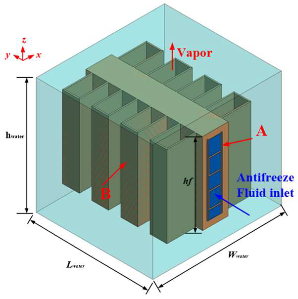
Six water evaporators, Hex–Hex5, are designed with different internal channels and external fins, as shown in

Table 4. Configuration of water evaporators.

Type	Internal Channels	External Fins
Hex0	A1	B1
Hex1	A1	B2
Hex2	A2	B2
Hex3	A3	B2
Hex4	A4	B2
Hex5	A5	B2

.

3. Numerical Model

3.1. Governing Equations of Boiling Water Side

The multiphase VOF model can simulate immiscible fluid flow by solving the momentum equation and tracking the fluid volume fraction in the control volume [26]. The transport equations governing the flow of liquid and vapor are formulated according to the VOF method. The water boiling model is built using the multiphase VOF model in order to compare the heat transfer performance of Hex0–Hex5 [10,18,26].

The following assumptions are deduced: (1) The boiling heat transfer between the water side and the fin is the main heat transfer mechanism in the multiphase region. (2) In the multiphase region, it is assumed that the heating surface is stationary. (3) Water and vapor phases are supposed to be incompressible fluids with constant physical parameters. Based on above assumptions, the governing equations of the multiphase domain are established as follows:

(1)

Volume fraction

In each computational cell of the domain, α identifies the fraction of the cell occupied by the primary phase. In this paper, the volume fraction takes values of 1 in the vapor, 0 in the liquid, and 0 < α < 1 in cells that are cut by the interface. The volume fraction of the vapor phase is defined as:

$$\alpha =\frac{Vv}{V}$$

(1)

where V_v is the volume of vapor phase in the whole area, m³; V is the volume in the whole area, m³; α is the volume fraction of vapor phase.

In the VOF model, the interphase interface is obtained by solving the continuity equation. The equation for phase i is as follows [26]:

$$\frac{1}{{\rho }_i}\left[\frac{\partial ({\alpha }_i{\rho }_i)}{\partial t}+\nabla \left({\alpha }_i{\rho }_i{v}_i\right)\right]=S_{{\alpha }_i}+{\displaystyle \sum _{i=1}^n\left({\dot{m}}_{ij}-{\dot{m}}_{ji}\right)}$$

(2)

where ρ_i is the volume fraction of phase i; t is the time, s; v_i is the velocity of phase i, m/s; ${\dot{m}}_i{}_j$ is the mass rate of phase i to phase j, kg/s; ${\dot{m}}_{ji}$ is the mass rate of phase j to phase i, kg/s; S_αi is the source phase, kg/(s·m³); n is the number of phases.

(2)

Momentum equation

The momentum equation is consistent in the whole calculation domain, and the calculated velocity parameters are applicable to all phases [26].

$$\frac{\partial (\rho \overrightarrow{v})}{\partial t}+\nabla (\rho \overrightarrow{v}\overrightarrow{v})=-\nabla P+\left[\mu (\nabla \overrightarrow{v}+\nabla {\overrightarrow{v}}^T)\right]+\rho \overrightarrow{g}+\overrightarrow{F}$$

(3)

where P is static pressure, Pa; $\overrightarrow{F}$ is a momentum source term generated by surface tension; μ is the dynamic viscosity, Pa·s.

ρ and μ are as follows:

$$\rho =\alpha {\rho }_v+(1-\alpha ){\rho }_l$$

(4)

$$\mu =\alpha {\mu }_v+(1-\alpha ){\mu }_l$$

(5)

where ρ_l and ρ_v are liquid phase and vapor phase curvatures, respectively, kg/m³; μ_l and μ_v are liquid phase and vapor phase dynamic viscosities, Pa·s.

In the momentum equation, the gravity and volumetric surface tension force are taken into consideration. The continuum surface force model proposed by Brackbill et al. [26] has been implemented such that the addition of surface tension to the VOF calculation results in a source term. Furthermore, the surface tension can be expressed as a volume force using the divergence theorem in terms of the pressure jump across the surface. The momentum source can be written in as follows [26]:

$$\overrightarrow{F}={\sigma }_{vl}\frac{{\alpha }_l{\rho }_l{k}_v\nabla {\alpha }_l+{\alpha }_v{\rho }_v{k}_l\nabla {\alpha }_v}{0.5({\rho }_l+{\rho }_v)}$$

(6)

where ${\sigma }_{vl}$ is the surface tension, N/m; ρ is density, $\rho ={\alpha }_l{\rho }_l+{\alpha }_v{\rho }_v$, kg/m³; k_v and k_l are the liquid phase and vapor phase curvatures, respectively, 1/m, k_v = −k_l; α is the volume fraction,$\nabla {\alpha }_v=-\nabla {\alpha }_l$.

(3)

Energy equation

In the VOF model, all phases use the same energy equation in Equation (7) [27].

$$\frac{\partial \left(\rho E\right)}{\partial t}+\nabla \left[\overrightarrow{v}(\rho E+P)\right]=\nabla (k_{eff}\nabla T)+S_h$$

(7)

where E is the specific energy, J/kg; T is temperature, K; k_eff is thermal conductivity, and W/(m·K); S_h is the initial heat source, J/(s·m³).

$$E=\frac{{\alpha }_l{\rho }_l{E}_l+{\alpha }_v{\rho }_v{E}_v}{{\alpha }_l{\rho }_l+{\alpha }_v{\rho }_v}$$

(8)

where E_v and E_l are the specific energy of the vapor phase and liquid phase, J/kg, respectively.

(4)

Rohsenow boiling model

The empirical correlation provided by Rohsenow is used to calculate the surface heat flux during boiling [28]:

$$q_{bw}={\mu }_l{h}_{lat}\sqrt{\frac{g({\rho }_l-{\rho }_v)}{\sigma }}{\left[\frac{C_{pl}(T_w-T_{sat})}{C_{qw}{h}_{lat}{\mathrm{Pr}}_{\mathrm{l}}^{n_p}}\right]}^{3.03}$$

(9)

where μ_l is the dynamic viscosity of the liquid phase, Pa·s; h_lat is the latent heat in the liquid phase, kJ/kg; C_pl is the specific heat of the liquid phase, J/(kg·K); ρ_l is the density of the liquid phase, kg/m³; P_rl is the Prandtl number; n_p is the Prandtl index and 1.73 in this paper; g is gravity, m/s²; ρ_v is steam density, kg/m³; σ is the surface tension coefficient of the liquid-gas interface, N/m, and is 0.072 N/m in this paper; T_w is the wall temperature, K; T_sat is the saturation temperature, K; C_qw is the empirical coefficient varying with the combination of liquid surfaces.

The Hertz-Knudsen equation is used to obtain the mass flow rate at the gas liquid interface [29]:

$$\left|S\right|=\phi \sqrt{\frac{M}{2\pi R}}\left[\frac{{\mathrm{P}}_{\mathrm{v}}}{\sqrt{T_v}}-\frac{{\mathrm{P}}_{\mathrm{sat}}\left(T_l\right)}{\sqrt{T_l}}\right]$$

(10)

In the saturated state, the relationship between pressure and temperature can be established with the Clausius-Clapeyron equation [30]:

$$\frac{dP}{dT}=\frac{h_{lat}}{T(\frac{1}{{\rho }_v}-\frac{1}{{\rho }_l})}$$

(11)

Then, the mass transport can be realized by the mass source term in the volume fraction equation of the VOF model. The evaporation processes are simplified concerning the mass transfer model as follows:

$$S_v=h_{l}at{\alpha }_l{\rho }_l(T_l-T_{sat})/T_{sat},T_l>T_{sat}$$

(12)

where S_v is the mass transfer rate of the vapor phase, kg/s.

3.2. Governing Equations of Antifreeze Side

For simplifying the calculation, the following assumptions are made: (1) The antifreeze is a three-dimensional Newtonian fluid. (2) The thermophysical properties of the antifreeze are assumed to be constant. (3) Non-slip velocity boundary condition is applied on the channel walls. (4) The viscous dissipation and radiation heat transfer are ignored. In most of the following simulations, Re is lower than 2300, hence, laminar flow is considered for all cases. Based on the above assumptions, the governing equations of the fluid domain are as follows [31]:

(1)

Continuity equation for antifreeze region:

$$\nabla \overrightarrow{u}=0$$

(13)

where, $\overrightarrow{u}$ is the velocity vector.

(2)

Momentum equation for antifreeze region:

$$\rho (\overrightarrow{u}\cdot \nabla )\overrightarrow{u}=-\nabla p+\mu {\nabla }^2\overrightarrow{u}$$

(14)

where μ is dynamic viscosity, Pa·s; ρ is antifreeze density, kg/m³; p is the pressure, MPa.

(3)

Energy equation for antifreeze region

$$\rho c_p\nabla \cdot (\overrightarrow{u}T)={\lambda }_f\nabla \cdot (\nabla T)$$

(15)

where T is the temperature of antifreeze, K; ${\lambda }_f$ is the thermal conductivity of antifreeze, and W/(m·K); $c_p$ is the specific heat of antifreeze, J/(kg·K).

In the solid region:

$${\lambda }_w\frac{{\partial }^{2}T}{\partial x^2}=0$$

(16)

where is λ_w the thermal conductivity of solid, W/(m·K).

3.3. Boundary Conditions and Initial Conditions

The computational domain is set up according to the structure in Figure 1. The top wall of the water side is set as the pressure outlet boundary, and the pressure is set as 7 kPa. The mass flow at the inlet of the antifreeze side is 10.8 kg/h, and the inlet temperature of antifreeze is 85 °C. The physical parameters of antifreeze are shown in

Table 5. Physical parameters of antifreeze and water.

Fluid	Density (kg/m3)	Specific Heat (J/kg·K)	Thermal Conductivity (W/m·K)	Viscosity (Pa·s)
Water	997.6	4182	0.62	8.9 × 10−4
Antifreeze	1056	3317	0.3937	6.2 × 10−4

.

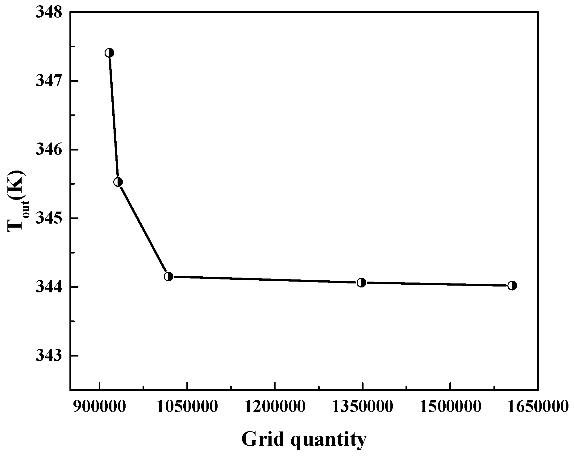
3.4. Grid Independence

The grid accuracy can be decided by comparing the outlet temperature of the antifreeze, T_out, acquired with a different grid quantity. In Figure 5, T_out gradually decreases with the increase of grid quantity. When the grid quantity is large enough, the outlet temperature tends to gradually become stable. Finally, the number of grids is 1.65 × 10⁶ in this study.

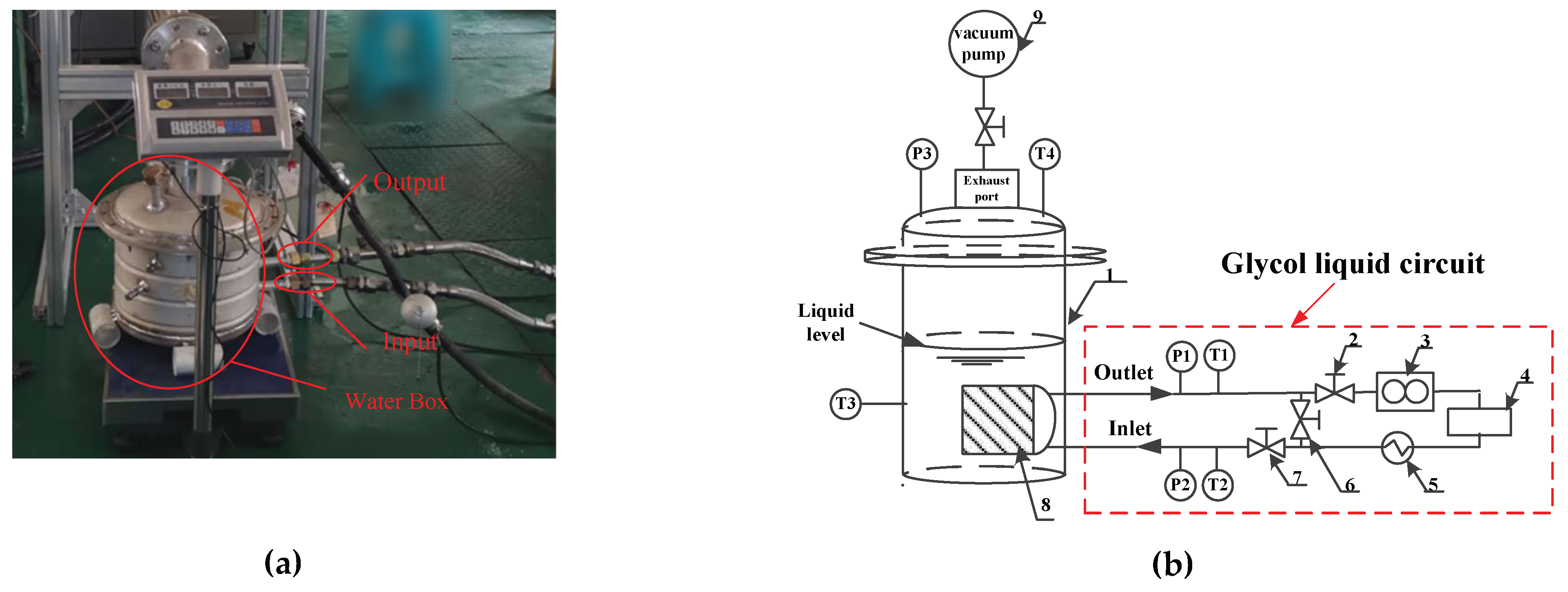
4. Experimental Methodology

4.1. Experimental Procedure

The experimental system is shown in Figure 6. It included a water evaporator, a low-pressure water tank, a vacuum pumper, a single-phase glycol liquid (65%) circuit and a data acquisition unit. Before the experiment, the water evaporator was placed in the water tank, and then the upper end cover was sealed by rubber rings and flanges. The glycol liquid circuit was connected to the water evaporator inside the water tank.

The cylindrical aluminum water tank with a diameter of 325mm and a height of 272 mm was used to store purified water. Hex0 was inside the water tank under sub-atmosphere pressure, and the liquid surface of water was always higher than Hex0. In addition, this experiment was carried out at the indoor temperature of about 38 °C. In Figure 6, the tank was insulated with insulation material. Thus, the heat exchange between the water tank and the atmosphere was ignored in the experiment data analysis.

The data acquisition unit consisted of flowmeter, temperature sensors and pressure sensors. The turbine flowmeter (LWJ) measured the mass flow of glycol liquid, and its measurement range and accuracy were 0–3000 kg/h and ± 0.5%, respectively. The pressure sensor (KYB600) was placed on the upper end cover of water tank to measure the pressure in the water tank, and its measurement range and accuracy were 0–600 kPa and ± 0.25%, respectively. The temperature sensors (WZPK-336) measured the water temperature in the tank and the inlet and outlet temperatures of glycol liquid. Their measurement range and accuracy were −50–+300 °C and class A, respectively.

Pure water was used as the phase change, and the pressure in the tank was controlled at 7 kPa. Antifreeze with a pressure of 0.2 MPa at 85 °C was pumped into the water evaporator. The flow rate of antifreeze flow was 800 kg/h.

4.2. Experimental Uncertainty Analysis

By measuring flow rate, the fluid inlet and outlet temperatures, the heat transfer (Q_f) and the convective heat transfer coefficient (h_f) can be calculated with Equations (17)–(19). The heat exchange released by the antifreeze can be calculated as follows:

$$Q_f=\dot{m}{c}_p(T_{in}-T_{out})$$

(17)

where Q_f is the heat exchange released by the antifreeze, W; $\dot{m}$ is the mass flow rate of the antifreeze, kg/s; $c_p$ is the specific heat of the antifreeze, J/(kg·K); T_out and T_in are the inlet and outlet temperatures of the antifreeze, respectively, K.

In this study, the average temperature of the antifreeze (T_m) is the average value of the inlet temperature (T_in) and the outlet temperature (T_out).

The flow in this experiment is a laminar flow, and Pr_f is 20.4. Sieder Tate equation is applicable to the laminar flow with Pr_f of 0.48–16700 [31].

The Nusselt number for antifreeze is calculated using the Sieder Tate Equation (18) [32]:

$$N{u}_f=1.86(\frac{{\mathrm{Re}}_f{\mathrm{Pr}}_f}{l/D_h}{)}^{\raisebox{1ex}{$1$}\!\left/ \!\raisebox{-1ex}{$3$}\right.}{(\frac{{\eta }_f}{{\eta }_w})}^{0.14}$$

(18)

where ${\mathrm{Pr}}_f$ is the Prandtl number of the fluid; Re_f is the Reynolds number of the fluid: The range of η_f/η_w is 0.0044-9.75, the value is 1 in this paper.

Then, the convective heat transfer coefficient for antifreeze can be calculated:

$$h_f=\frac{{\lambda }_f}{d_e}N{u}_f$$

(19)

where λ_f is thermal conductivity for the antifreeze, W/(m·K); d_e is the equivalent diameter, m;

We ignore the heat exchange with the environment, the heat absorbed by the water is equal to the heat released by the antifreeze. Assuming that the wall temperature is approximately constant under the action of water phase change, the average wall temperature (T_w) can be calculated using the logarithmic mean temperature difference [33]:

$$\frac{Q_f}{A_{sur}{h}_f}=\frac{T_{in}-T_{out}}{\ln \frac{T_{out}-T_w}{T_{in}-T_w}}$$

(20)

where $T_w$ is the channel average wall temperature, K; $A_{sur}$ is the total heat transfer area of the channel, m².

The boiling heat transfer coefficient is calculated:

$$h_{sat}=\frac{Q_f}{A_{sat}(T_w-T_{sat})}$$

(21)

where $T_{sat}$ is the saturation temperature of the water, K. A_sat is the heat exchange area of the boiling side, m².

The thermal conductivity of the channel wall is much smaller than the convection and boiling heat transfer coefficients; so, the heat transfer coefficient (K) can be given by:

$$K=\frac{1}{\frac{1}{h_f}+\frac{1}{h_{sat}}}$$

(22)

Before the experiments on the water evaporator, the temperatures and flow rates were calibrated with appropriate instruments. The parameters in this experiment are divided into direct measurement parameters and calculation parameters; the uncertainty of direct measurement parameters is calculated by the measuring range and accuracy of the measuring instrument and is calculated by Equation (23). The uncertainty of the calculation parameters is calculated by Equation (24) based on the uncertainty of the direct measurement parameters [34,35].

$$\xi M=\frac{M_R\times \epsilon }{M}$$

(23)

$$\delta R=\sqrt{{\displaystyle \sum _{i=1}^n{\left(\frac{\partial R}{\partial x_i}\delta x_i\right)}^2}}$$

(24)

where M, M_R, ε, i, n, δR, δx_i are the direct measurement parameter, the measuring range of measuring equipment, the measurement accuracy, the specific parameter counter, the number of the independent variables, uncertainties associated with the dependent variables, R, and independent variables, $x_i$. Therefore, the calculated uncertainty of $\dot{m}$, P, T_in-T_out, T_sat, T_w, $h_{sat}$, Q, $h_f$ are 1.23%, 2.54%, 1.6%, 1.3%, 2.38%, 3.71%, 2.02% and 1.26%, respectively.

4.3. Experimental Validation

Experiment was carried out using Hex0 to verify the numerical model. The experimental and simulation data were obtained under the same boundary conditions. The comparison of the two results is as follows.

$$error=\frac{\left|Exp-Sim\right|}{Exp}$$

(25)

where error is the relative error; Exp and Sim represent experimental and simulation data, respectively.

From

Table 6. Comparison of experimental and simulation results.

	Experiment	Simulation	Error
Tout (°C)	48	50.56	5.06%
K (W·m−2·K−1)	1500	1562	3.9%
hf (W·m−2·K−1)	2876	3020.1	5.01%
Qf (kW)	29	30.1	3.78%

, it can be seen that the numerical results match well with the experimental ones with the errors of 3.8%, 4.53%, 5.01% and 3.78% for T_out, K, h_f and Q, respectively.

5. Analysis of Simulation Results

After the simulation model is verified, the heat transfer performances of water evaporators are simulated in 7 kPa sub-atmospheric environment. The results are discussed as follows.

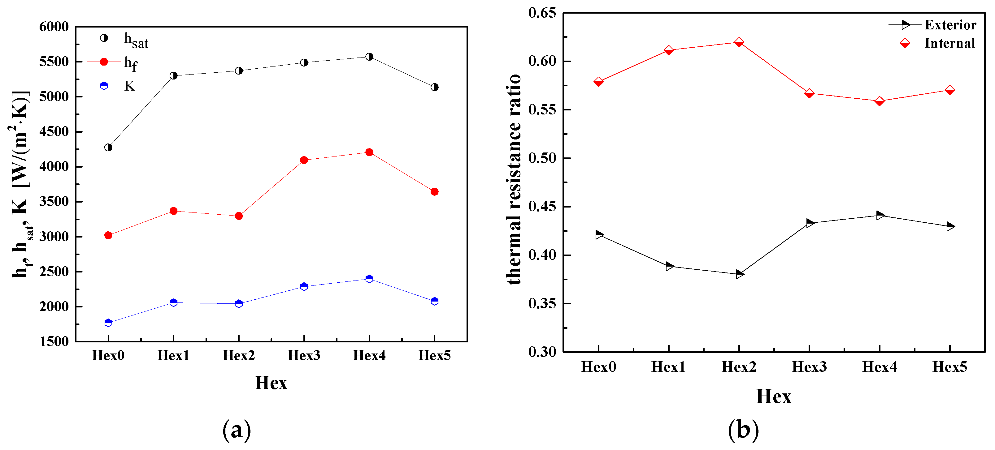
5.1. Heat Transfer Coefficient and Thermal Resistance

The variations of K, $h_f$, $h_{sat}$ and the ratio of thermal resistance for water evaporators are shown in Figure 7.

Figure 7a depicts the effects of different channels and fins on the heat transfer coefficient, and the following conclusions can be obtained:

Hex0 and Hex1 have the same internal channel A1, with different external fins B1 and B2. h_sat of Hex0 is 4276.45 W/(m²·K) and h_sat of Hex1 is 5300 W/(m²·K). h_sat and K of Hex1 increases by about 19.32% and 14% compared to that of Hex0, respectively. It can be observed that heat transfer performance can be enhanced by adding ribs to the fin.

The structural difference between Hex1 and Hex2 is only that the internal channel A1 is continuous and A2 is discontinuous. The differences of h_f, h_sat and K between Hex1 and Hex2 are small. So, it can be concluded that the structural continuity of the internal channel has little impact on the heat transfer performance.

Hex2 and Hex3, Hex4 and Hex5 have the same external fin B2 with different wave height. The wave height of Hex2 and Hex4 is two times that of Hex3 and Hex5, respectively. The K of Hex3 is improved by about 10.71% compared to Hex2. The K of Hex4 is improved by about 13.31% compared to Hex5. Therefore, the heat transfer performance can be improved by changing the wave height of the internal channel.

For Hex2–Hex5, they have the same external fin B2, but with different internal channels. h_f, K of Hex5 is 6.78% and 1% higher than that of Hex2, respectively. But h_f, K of Hex4 is 2.71% and 4.55% higher than that of Hex3, respectively. Therefore, the shape change of the single-phase liquid side channels can affect the heat exchange performance.

The other important parameter evaluating the water evaporator performance is the thermal resistance. Figure 7b depicts the variations in the internal and exterior thermal resistance with change in the structure of the water evaporator. The ratios of internal thermal resistance to the heat transfer coefficient of Hex0–Hex5 are all higher than 55%. It indicates that enhanced heat transfer design for the antifreeze side should receive more attention. Besides, changing the fin shape can reduce the internal thermal resistance, for example, compared with Hex2 and Hex4, the maximum internal thermal resistance can be reduced by 14.5%.

5.2. Velocity Distribution of Antifreeze Side

Different flow channel structures lead to different flow patterns, which in turn affects the heat transfer performance. Through the analysis of the heat transfer coefficient of internal fins, it is known that the discontinuity of fins has little impact on heat transfer for OSF geometry and the heat transfer performances of fin A1 and fin A2 are basically same. Hence, this part only shows the flow and heat transfer characteristics of internal fins A2–A5.

The velocity distributions of single-phase antifreeze in different fin internal channel structures are shown in Figure 8. The red dotted lines in Figure 8a,b mark the fin discontinuity clearly, and the oval lines in Figure 8c,d mark the changes in flow near the fins clearly. The maximum velocity in Figure 8a,b are 0.476 m/s and 0.214 m/s, respectively. The maximum velocity in Figure 8c,d are 0.848 m/s and 0.411 m/s, respectively. This velocity difference is mainly caused by different fin height, fin shape and fin discontinuity.

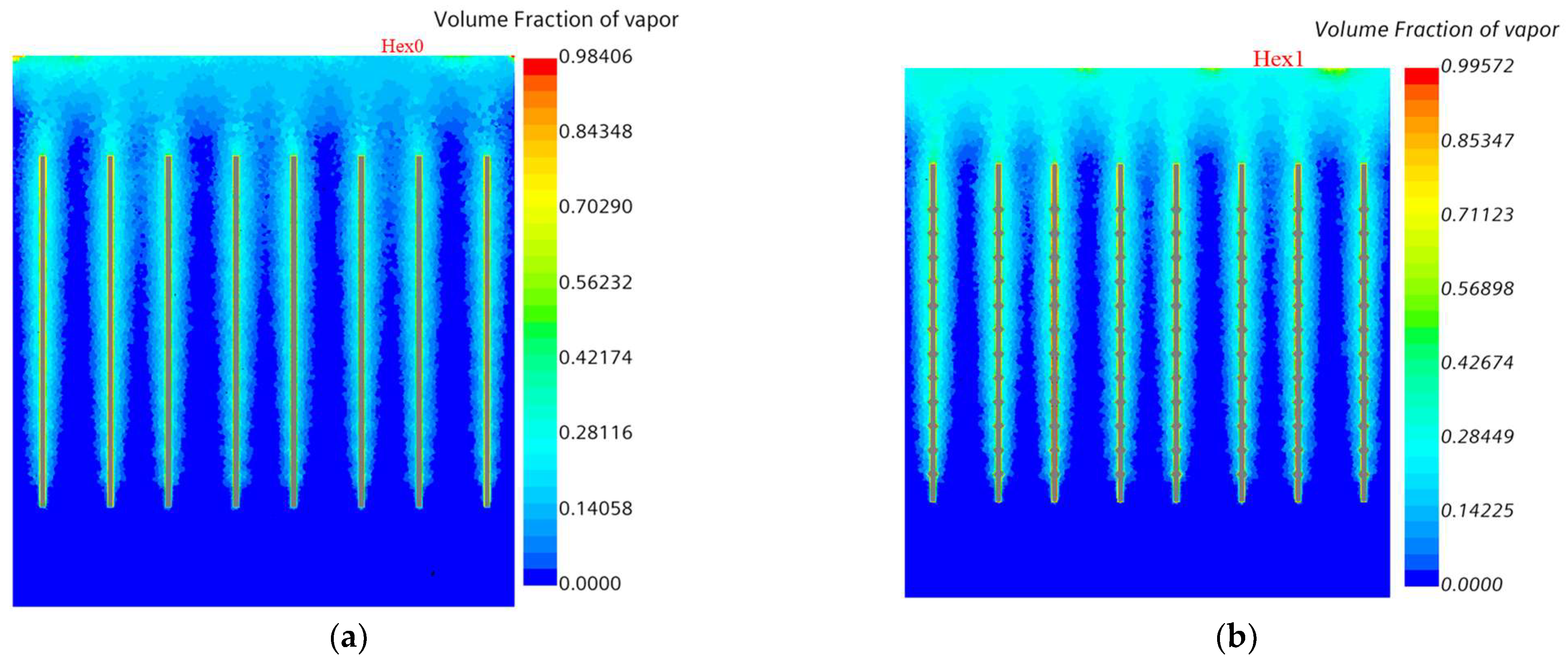
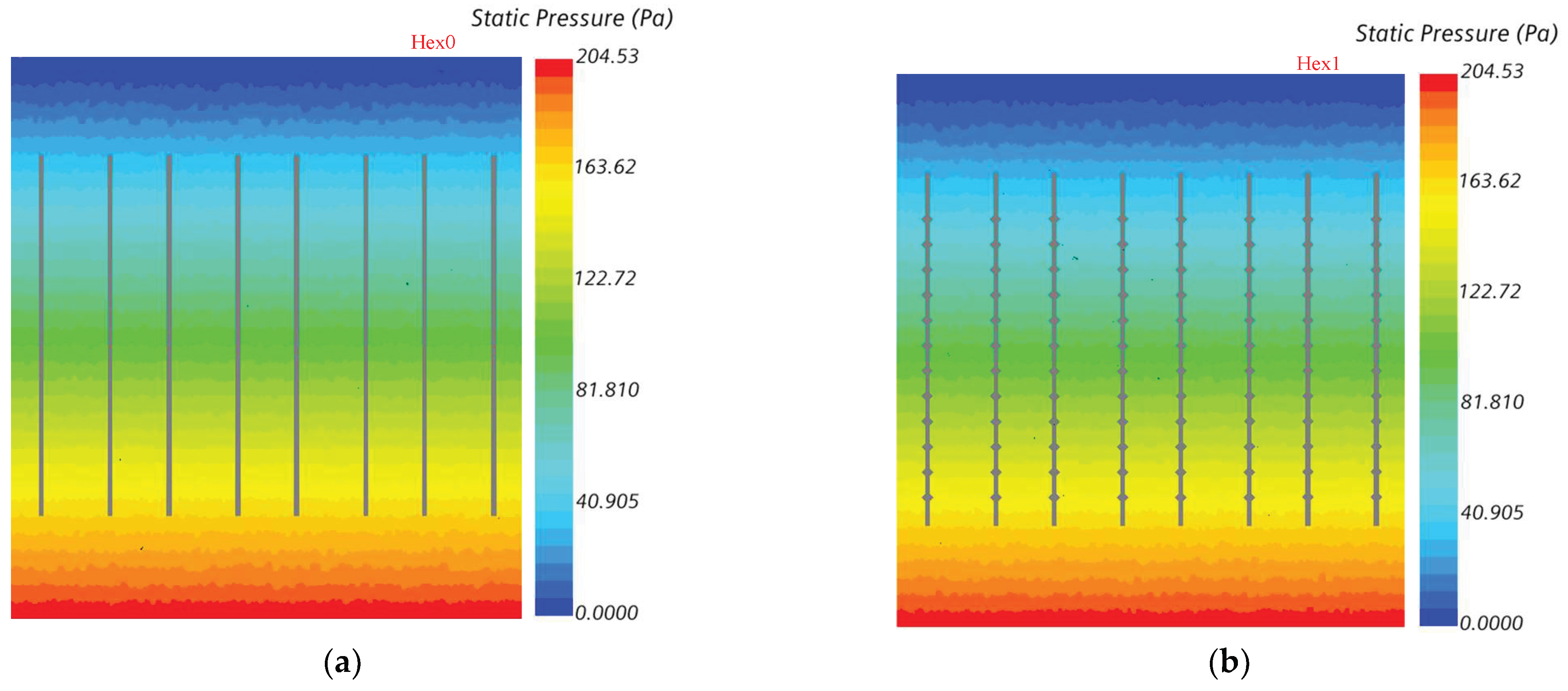
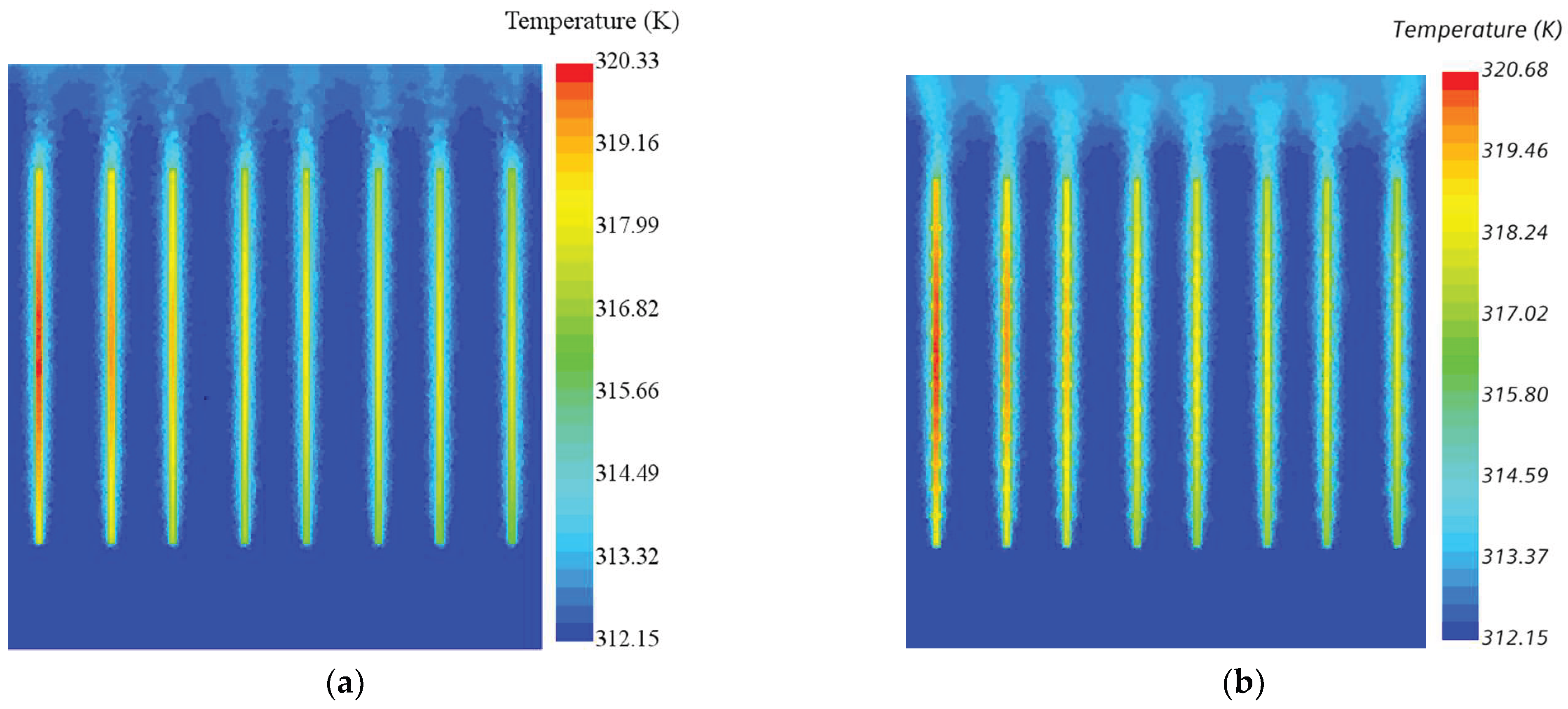
5.3. Volume Fraction and Static Pressure at Boiling Water Side

In order to compare the effects of external fins B1 and B2 on pool boiling heat performance, Hex0 and Hex1 are selected due to their having the same internal channel A1, but with different external fins B1 and B2. The section located 5 mm away from the internal channel are selected. The results of the volume fraction, temperature distribution and static pressure are shown in Figure 9, Figure 10 and Figure 11 respectively.

From Figure 9, we can observe that the volume fraction of vapor decreases gradually from top to bottom in the vertical direction. This phenomenon is mainly caused by the static pressure of water, which in turn affects the saturation temperature of water. In this paper, the static pressure values of Hex0 and Hex1 are the same and are 204.53 Pa, as shown in Figure 10. In previous studies [33], it was pointed out that the saturation temperature of water increases by about 10 °C for every 1 kPa increase of static pressure, which has an obvious impact on low-pressure boiling heat transfer.

In addition, the volume fraction of Hex1 is greater than the one of Hex0 in Figure 9. More steam can be generated in Hex1 than Hex 0, mainly because the heat exchange area of external fin B2 is larger than that of external fin B1. The fin wall temperature of Hex1 is higher than that of Hex0, as shown in Figure 11. This makes the temperature difference between the saturated temperature and water in Hex1 larger than that in Hex0, which makes the heat transfer more intense. Therefore, under the same condition, adding ribs on the fins is conducive to enhancing the heat transfer performance.

5.4. Optimal Combination Structure for Water Evaporator

The pressure drops of Hex0~Hex5 at the inlet and the outlet of antifreeze are shown in Figure 12. The pressure drop of Hex5 with the internal channel A4 is the largest because its fin wave height is the smallest. The pressure drop of Hex4 is about 420 Pa. The pressure drops of Hex0, Hex1 and Hex2 are about 25 Pa. The pressure drops of Hex5 and Hex3 are 116 Pa and 106 Pa, respectively. Therefore, the pressure drop of the OSF structure is the smallest.

The heat transfer coefficients and pressure drops of Hex0~Hex5 are shown in Figure 13. The heat transfer coefficient of Hex3 is 2288.76 W/(m²·K) and that of Hex4 is 2397.37 W/(m²·K), and the value of Hex4 is about 1.05 times that of Hex3, but the pressure drops of Hex4 is 3.52 times that of Hex3. Although the pressure drops of Hex0~Hex2 are smaller than the one of Hex4, their heat transfer coefficients are smaller than the one of Hex3. For the heat exchanger, the heat transfer coefficient has a greater impact on the heat transfer performance than the pressure drop. The heat transfer coefficient of Hex4 is 1.35 times, 1.16 times, 1.17 times and 1.15 times that of Hex0, Hex1, Hex2 and Hex5, respectively. Considering the pressure drop and the heat transfer coefficient, for the aircraft, the optimal design structure of the water evaporator is Hex4. Hex4 has the largest heat transfer coefficient and smallest weight, which can decrease the structure and weight and reduce the weight compensation of the aircraft.

6. Conclusions

In this paper, the VOF method is used to compare the heat transfer performance of six kinds of water evaporators, and the effects of different fin structures and combined configurations of water evaporators on the heat transfer performance are revealed. The above points can be summarized as follows:

(1)

The comparison of experimental and simulation results shows that the built numerical models can satisfy the accuracy requirements of sub-atmospheric boiling study in the water evaporator.

(2)

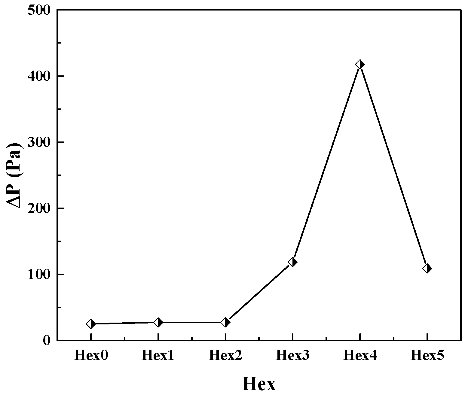
The heat transfer performances of five internal channel structures are compared. It is concluded that the change of channel continuity has little effect on the heat transfer performance. The height reduction of the channel wave is beneficial for improving the heat exchange performance, but it will increase the pressure drop accordingly. The pressure drop increases about two times with a height reduction of one half. The change of the internal channel shape can lead to a change in the heat exchange characteristics.

(3)

The heat transfer performances of the two external fin structures (B1 and B2) are analyzed. It is concluded that adding ribs to the fins is conducive to enhancing the heat transfer performance, which can improve the boiling heat transfer performance by about 13.31%. Meanwhile, the influence of water static pressure cannot be ignored in study of heat transfer performance in a sub-atmospheric environment.

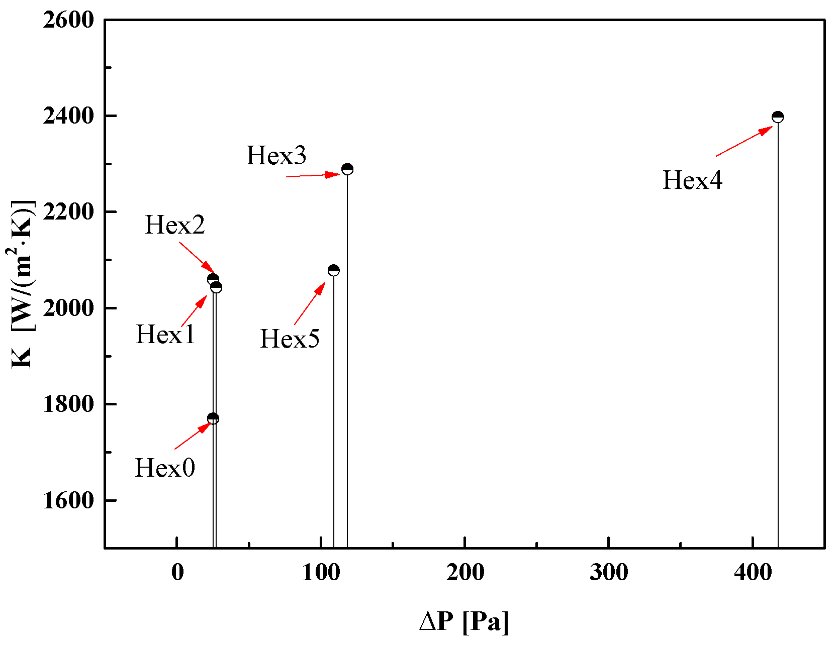
(4)

Comparing the heat transfer coefficients of different structural water evaporators, the heat transfer coefficient of Hex4 is 1.35 times, 1.16 times, 1.17 times and 1.15 times larger than the ones of Hex0, Hex1, Hex2 and Hex5, respectively. For the aircraft, the best design of a water evaporator is Hex4.

References

1. Glass, D. Ceramic Matrix Composite (CMC) Thermal Protection Systems (TPS) and Hot Structures for Hypersonic Vehicles. In Proceedings of the 15th AIAA International Space Planes and Hypersonic Systems and Technologies Conference, Dayton, OH, USA, 28 April–1 May 2008. [Google Scholar]
2. Jackson, T.A.; Eklund, D.R.; Fink, A.J. High speed propulsion: Performance advantage of advanced materials. J. Mater. Sci. 2004, 39, 5905–5913. [Google Scholar] [CrossRef]
3. Esser, B.; Barcena, J.; Kuhn, M.; Okan, A.; Haynes, L.; Gianella, S.; Ortona, A.; Liedtke, V.; Francesconi, D.; Tanno, H. Innovative Thermal Management Concepts and Material Solutions for Future Space Vehicles. J. Spacecr. Rocket. 2015, 53, 1051–1060. [Google Scholar] [CrossRef] [Green Version]
4. Kellermann, H.; Lüdemann, M.; Pohl, M.; Hornung, M. Design and Optimization of Ram Air-Based Thermal Management Systems for Hybrid-Electric Aircraft. Aerospace 2021, 8, 3. [Google Scholar] [CrossRef]
5. Wang, R.; Dong, S.; Jiang, H.; Li, P.; Zhang, H. Parameter-Matching Algorithm and Optimization of Integrated Thermal Management System of Aircraft. Aerospace 2022, 9, 104. [Google Scholar] [CrossRef]
6. Kandlikar, S.G.; Colin, S.; Peles, Y.; Garimella, S.; Pease, R.F.; Brandner, J.J.; Tuckerman, D.B. Heat transfer in microchannels-2012 status and research needs. J. Heat Transf. 2013, 135, 942–955. [Google Scholar] [CrossRef] [Green Version]
7. Jiang, X.Y.; Liu, M.; Wu, H.; Zheng, Y.; Zhuang, J. Numerical Study on Low-Temperature Region as Heat Sink and Its Heat Dissipation Capacity for Hypersonic Vehicle. Aerospace 2021, 8, 238. [Google Scholar] [CrossRef]
8. Zhang, X.J.; Zhang, Z.Q.; Gao, F. Fuel temperature analysis of advanced fighter aircraft during supersonic cruise. J. Aerosp. Power 2010, 2, 0258-06. [Google Scholar]
9. Das, A.; Das, P.; Saha, P. Some investigations on the enhancement of boiling heat transfer from planer surface embedded with continuous open tunnels. Exp. Therm. Fluid Sci. 2010, 34, 1422–1431. [Google Scholar] [CrossRef]
10. Chan, M.A.; Yap, C.R.; Ng, K.C. Pool Boiling Heat Transfer of Water on Finned Surfaces at Near Vacuum Pressures. J. Heat Transf. 2010, 132, 031501. [Google Scholar] [CrossRef]
11. Magnini, M.; Matar, O. Numerical study of the impact of the channel shape on microchannel boiling heat transfer. Int. J. Heat Mass Transf. 2020, 150, 119322. [Google Scholar] [CrossRef]
12. Webb, R.L. Odyssey of the Enhanced Surface. ASME J. Heat Transf. 2004, 126, 1051–1059. [Google Scholar] [CrossRef]
13. McGillis, W.R.; Fitch, J.S.; Hamburgen, W.R.; Carey, V.P. Pool Boiling Enhancement Techniques for Water at Sub-atmosphere. In WRL Research Report 90/9; Western Research Laboratory: Palo Alto, CA, USA, 1990. [Google Scholar]
14. Wen, M.-Y.; Ho, C.-Y. Pool boiling heat transfer of deionized and degassed water in vertical/horizontal V-shaped geometries. Heat Mass Transf. 2003, 39, 729–736. [Google Scholar] [CrossRef]
15. Han, J.; Zhang, Y. High performance heat transfer ducts with parallel broken and V-shaped broken ribs. Int. J. Heat Mass Transf. 1992, 35, 513–523. [Google Scholar] [CrossRef]
16. Pastuszko, R.; Kaniowski, R.; Wójcik, T.M. Comparison of pool boiling performance for plain micro-fins and micro-fins with a porous layer. Appl. Therm. Eng. 2020, 166, 114658. [Google Scholar] [CrossRef]
17. Jiang, H.; Yu, X.; Xu, N.; Wang, D.; Yang, J.; Chu, H. Effect of T-shaped micro-fins on pool boiling heat transfer performance of surfaces. Exp. Therm. Fluid Sci. 2022, 136, 110663. [Google Scholar] [CrossRef]
18. Giraud, F.; Rulliere, R.; Toublanc, C.; Clausse, M.; Bonjour, J. Experimental evidence of a new regime for boiling of water at sub-atmospheric pressure. Exp. Therm. Fluid Sci. 2015, 60, 45–53. [Google Scholar] [CrossRef]
19. Ramaswamy, C.; Joshi, Y.; Nakayama, W.; Johnson, W.B. Effects of Varying Geometrical Parameters on Boiling From Microfabricated Enhanced Structures. J. Heat Transf. 2003, 125, 103–109. [Google Scholar] [CrossRef]
20. Pal, A.; Joshi, Y. Boiling at sub-atmospheric conditions with enhanced structures. In Proceedings of the Thermal and Thermomechanical Proceedings 10th Intersociety Conference on Phenomena in Electronics Systems, San Diego, CA, USA, 30 May–2 June 2006; pp. 620–629. [Google Scholar]
21. Chao, D.F.; Zhang, N.; Yang, W.-J. Nucleate Pool Boiling on Copper-Graphite Composite Surfaces and Its Enhancement Mechanism. J. Thermophys. Heat Transf. 2004, 18, 236–242. [Google Scholar] [CrossRef]
22. McNeil, D.; Burnside, B.; Rylatt, D.; Elsaye, E.; Baker, S. Shell-side boiling of water at sub-atmospheric pressures. Int. J. Heat Mass Transf. 2015, 85, 488–504. [Google Scholar] [CrossRef]
23. Zhang, Q.; Feng, Z.; Li, Z.; Chen, Z.; Huang, S.; Zhang, J.; Guo, F. Numerical investigation on hydraulic and thermal performances of a mini-channel heat sink with twisted ribs. Int. J. Therm. Sci. 2022, 179, 107718. [Google Scholar] [CrossRef]
24. Ding, B.; Zhang, Z.-H.; Gong, L.; Xu, M.-H.; Huang, Z.-Q. A novel thermal management scheme for 3D-IC chips with multi-cores and high power density. Appl. Therm. Eng. 2020, 168, 114832. [Google Scholar] [CrossRef]
25. Ajalingam, R.; Chakraborty, S. Effect of shape and arrangement of micro-structures in a microchannel heat sink on the thermo-hydraulic performance. Appl. Therm. Eng. 2021, 190, 116755. [Google Scholar]
26. Brackbill, J.; Kothe, D.; Zemach, C. A continuum method for modeling surface tension. J. Comput. Phys. 1992, 100, 335–354. [Google Scholar] [CrossRef]
27. Mohsin, M.; Kaushal, D.R. 3D CFD validation of invert trap efficiency for sewer solid management using VOF model. Water Sci. Eng. 2016, 9, 106–114. [Google Scholar] [CrossRef] [Green Version]
28. Rohsenow, W.M. A method of correlating heat transfer data for surface boiling of liquids. J. Heat Transfer. 1952, 74, 969–973. [Google Scholar] [CrossRef]
29. Schrage, R.W. A Thermal Study of Interface Mass Transfer; Columbia University Press: New York, NY, USA, 1953; pp. 160–256. [Google Scholar]
30. Knudsen, M. The Kinetic Theory of Gases, Some Modern Aspects. In Methuen’s Monographs on Physical Subjects; Methuen & Company Limited: London, UK, 1934. [Google Scholar]
31. Liu, X.; Yu, J. Numerical study on performances of mini-channel heat sinks with non-uniform inlets. Appl. Therm. Eng. 2016, 93, 856–864. [Google Scholar] [CrossRef]
32. Yang, S.M.; Tao, W.Q. Heat Transfer; Higher Education Press: Beijing, China, 2006. [Google Scholar]
33. Khoshvaght-Aliabadi, M.; Hormozi, F.; Zamzamian, A. Role of channel shape on performance of plate-fin heat exchangers: Experimental assessment. Int. J. Therm. Sci. 2014, 79, 183–193. [Google Scholar] [CrossRef]
34. Kline, S.J.; McClintock, F.A. Describing uncertainties in single-sample experiments. Mech. Eng. 1953, 75, 3–8. [Google Scholar]
35. Moffat, R.J. Describing the uncertainties in experimental results. Exp. Therm. Fluid Sci. 1988, 1, 3–17. [Google Scholar] [CrossRef]
Figure 1. Structure of water evaporator and its channels (A and B represent internal channels and external fins, respectively).
Aerospace 09 00697 g001
Figure 2. Structural dimensions of A1–A3 with OSF geometry. (a) A1 (b) A2 (c) A3.
Aerospace 09 00697 g002
Figure 3. Structural dimensions of A4 and A5 with WF geometry. (a) Front view (b) A4 (c) A5.
Aerospace 09 00697 g003
Figure 4. Structural shape of external fins. (a) B1, (b) B2.
Aerospace 09 00697 g004
Figure 5. Relationship of average outlet temperature with grid quantity.
Aerospace 09 00697 g005
Figure 6. Photo and schematic diagram of experiment system (1—water tank, 2,6 and 7—valve, 3—flowmeter, 4—glycol liquid reservoir, 5—liquid pump, 8—water evaporator, 9—vacuum pump, T1, T2, T3 and T4 are temperature sensor, P1, P2 and P3 are pressure sensor). (a) Photo, (b) schematic diagram.
Aerospace 09 00697 g006
Figure 7. Comparison of heat transfer performance for Hex0~Hex5 (a) hf, hsat and K (b) Thermal resistance ratio.
Aerospace 09 00697 g007
Figure 8. Velocity distribution of A2~A5. (a) A2 (h = 2.5 mm); (b) A3 (h = 1.2 mm); (c) A4 (h = 1.2 mm); (d) A5 (h = 2.5 mm).
Aerospace 09 00697 g008
Figure 9. Volume fraction contours of Hex0 and Hex1. (a) Volume fraction of Hex0 (b) Volume fraction of Hex1.
Aerospace 09 00697 g009
Figure 10. Static pressure comparison between (a) Hex0 and (b) Hex1.
Aerospace 09 00697 g010
Figure 11. Temperature contour comparison between (a) Hex0 and (b) Hex1.
Aerospace 09 00697 g011
Figure 12. Average pressure drop.
Aerospace 09 00697 g012
Figure 13. Pressure drop and heat transfer coefficient.
Aerospace 09 00697 g013