Design of an ATC Tool for Conflict Detection Based on Machine Learning Techniques

Abstract

Given the ongoing interest in the application of Machine Learning (ML) techniques, the development of new Air Traffic Control (ATC) tools is paramount for the improvement of the management of the air transport system. This article develops an ATC tool based on ML techniques for conflict detection. The methodology develops a data-driven approach that predicts separation infringements between aircraft within airspace. The methodology exploits two different ML algorithms: classification and regression. Classification algorithms denote aircraft pairs as a Situation of Interest (SI), i.e., when two aircraft are predicted to cross with a separation lower than 10 Nautical Miles (NM) and 1000 feet. Regression algorithms predict the minimum separation expected between an aircraft pair. This data-driven approach extracts ADS-B trajectories from the OpenSky Network. In addition, the historical ADS-B trajectories work as 4D trajectory predictions to be used as inputs for the database. Conflict and SI are simulated by performing temporary modifications to ensure that the aircraft pierces into the airspace in the same time period. The methodology is applied to Switzerland’s airspace. The results show that the ML algorithms could perform conflict prediction with high-accuracy metrics: 99% for SI classification and 1.5 NM for RMSE.

1. Introduction

In the same way that air traffic is constantly increasing, technological development is needed to deal with this air traffic demand. Single European Sky ATM Research (SESAR) is the European solution to tackle the evolution of the Air Traffic Management (ATM) system. One of the goals of SESAR is to research the feasibility of using new technologies in the ATM system [1] and, in particular, the Air Traffic Control (ATC) system. Automation is one of the pillars to ensure that traffic increases are managed safely [2]. This paper deals with this issue by developing a new data-driven approach for conflict detection between aircraft.

An accident is the worst event that can occur in ATM [3]. An accident means that the whole system and all safety barriers have failed. A conflict is a precursor of an accident. The ICAO defines a conflict as any situation involving aircraft and hazards in which the applicable separation minima may be compromised [4]. Then, it is crucial to avoid separation infringements that could lead, eventually, to a collision. Since the 1960s, several authors have developed different methods to study conflict and collision risk. Conflict and collision risk are metrics that analyse the level of safety for the ATM system. Reich [5,6] pioneered the development of collision risk modelling (CRM) for parallel routes in oceanic airspace. His work was paramount because it settled the pillars of collision risk based on random flight errors (positioning and velocity). Other authors have employed more or less complex techniques to evaluate collision and conflict risk [7,8,9,10,11]. The authors recommend the work of Netjasov and Janic [12] for a deeper review of CRM.

However, conflict detection differs from conflict risk because it is based on a tactical level (separation provision) instead of a strategic level (airspace design). Conflict detection tools aim to help Air Traffic Controllers (ATCos) to identify conflicts in the airspace. Besides this, conflict detection is typically studied at three different levels: long, mid-, and short term. This work analyses the mid- and short-term horizon (2–10 min) for ATC tools. ATC tools automatize conflict detection, helping ATCos in their labour to avoid separation infringements and reducing their workload. There are many different ATC tool models which were developed for conflict detection. Krozel et al. [13] stated that they can be divided into four areas depending on being static, being dynamic, uncertainty, and probability. Paielli et al. [14] developed a new approach based on tactical pairwise trajectory analysis. Other authors found their studies on complex probabilistic models to understand trajectory uncertainty [15,16,17,18].

Here, the applicability of data-driven approaches is analysed for conflict detection. Machine Learning (ML) is one of the branches that takes advantage of historical data. The European Aviation AI high-level group defines ML as “the ability of algorithms to learn from the input and output data that characterise them” [19]. The goal of ML algorithms is to learn patterns from historical situations (databases) that underline those situations. The output of the algorithm is to apply the learned rules to predict new situations. Typically, there are three types of ML algorithms depending on the input/output data required: supervised, non-supervised, and reinforcement learning. Supervised learning demands the output associated with the input data, unsupervised learning acquires patterns from the input data without knowing the output data, and reinforcement learning makes the model learn a sequence of decisions based on rewards and penalties. In addition, ML algorithms can be divided in turn into classification and regression problems. Classification problems separate samples into different classes (binary or multiclassification). Regression problems provide numerical predictions. The authors recommend the works [20,21] to understand these topics.

Aviation is a field with a huge amount of data that is increasingly available for research purposes. ML techniques take advantage of the data, and have recently been applied to different topics: trajectory prediction [22,23,24], airspace performance metrics [25,26] and atmospheric models [27,28]. One of the issues of employing a data-driven approach is conflict generation. Up until now, conflict simulation has used different methods. Top-down models generate customised conflicts in advance, based on predefined situations [29]. Other approaches perform simulations adding uncertainty to different operational variables (wind, weight, velocity, etc.) [29,30,31,32]. The goal is to obtain an extensive database with enough separation infringements, which is not trivial.

Therefore, this work aims to develop the pillars of a further ATC tool for conflict detection based on ML techniques. One of the strong points is the addition of Four-Dimension Trajectory (4DT) predictions based on historical ADS-B trajectories. This allows us to improve the ability to predict conflicts based on 4DT predictions. After the introduction, the framework for the ATC tool based on ML techniques is presented, and the data-driven approach is explained for the extraction of trajectories to constitute the database. Section 3 details the selected ML techniques and the process followed in order to apply them. Section 4 shows the results obtained for the classification and regression techniques. Conclusions are presented in Section 5.

2. Framework for ATC Tools Based on ML Techniques

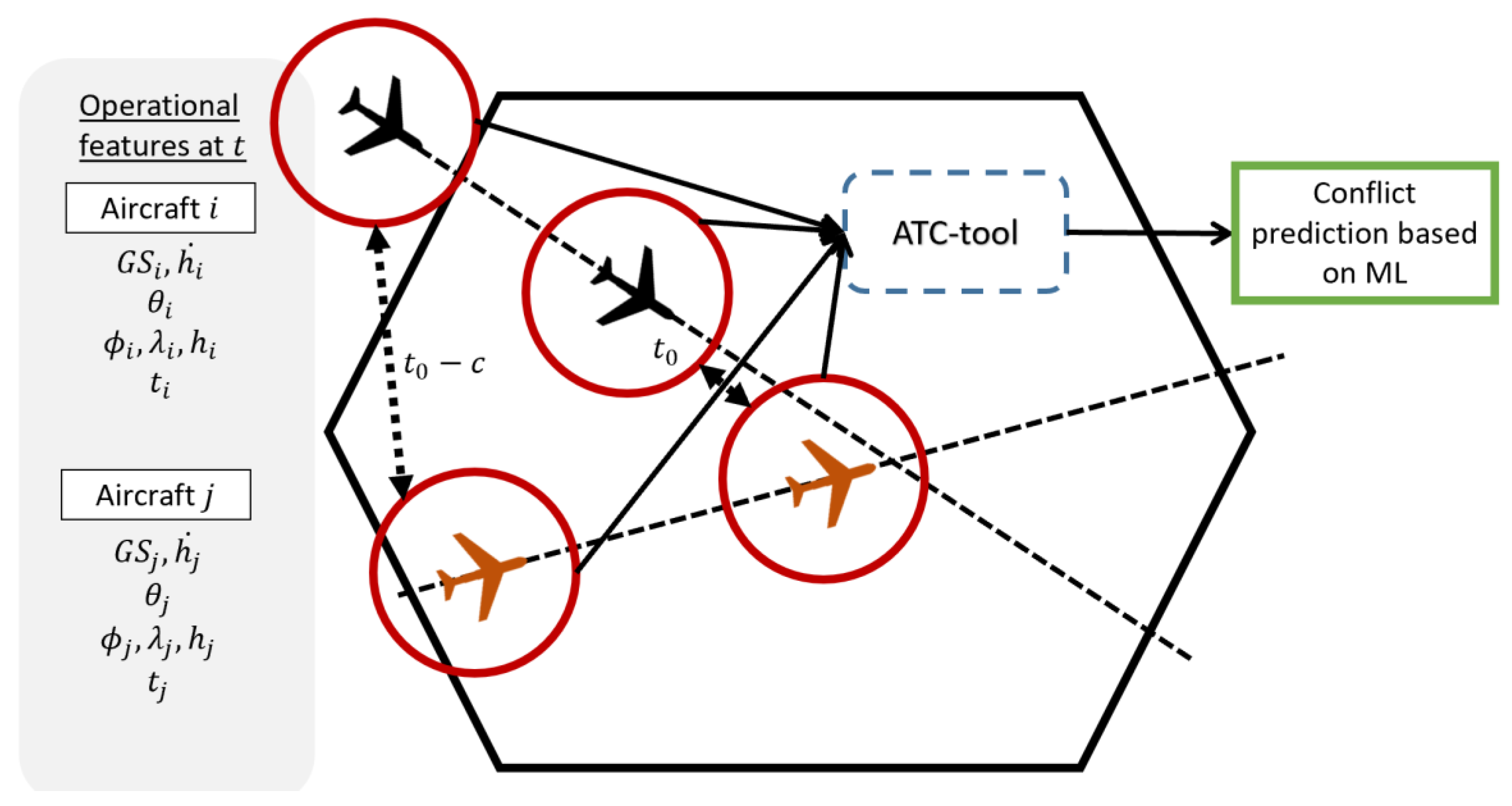
A conflict detection ATC tool aims to provide information to the ATCo about aircraft pairs which are expected to infringe the separation minima. The ATC tool developed in this work is based on a data-driven approach using ML techniques. Here, it is essential to note that the ATC tool provides predictions focusing on conflict detection but not trajectory prediction. This means that the ML model does not perform the trajectory prediction, nor does it afterwards analyse if a conflict could occur; it performs the conflict prediction based on what happened in previous situations. This novel approach employs ML algorithms to learn the underlying factors that lead to separation infringement by including historical 4D trajectories as predictions. The primary characteristics and hypothesis are the following:

• The ATC tool makes predictions based on the evolution of the aircraft throughout the airspace. The predictions depend on the time $\left(t\right)$ and the operational features of both aircraft. The ATC tool updates the prediction every $c$ minutes.
• The ATC tool obtains the aircraft within the sector and the aircraft in proximity of the airspace that will penetrate the airspace in the following $m$ minutes. $c$ and $m$ values should be defined by Air Navigation Service Providers (ANSPs) in advance.
• The ATC tool receives a 4DT prediction for each aircraft based on historical data and the operational features (state vector) based on ADS-B data. The ML model uses both inputs.
• The ATC tool was developed for the tactical ATCo, which continuously monitors the state of the aircraft throughout the airspace.
• The ATC tool does not provide information on conflict resolution.

Figure 1 represents the operational concept of the ATC tool. Both aircraft $i$ and $j$ are flying in the airspace. The ATC tool performs conflict prediction between them, along with other aircraft flying in the airspace and the aircraft that will pierce in $m$ minutes. The ATC tool demands two types of information: the state vector at the moment of the prediction and 4DT predictions. The state vector of each aircraft is accessible by different data sources based on ADS-B. However, the main problem is obtaining 4DT predictions of the aircraft. Typically, 4DT predictions are calculated by the ground server or provided by the aircraft throughout the flight. We do not have access to this type of prediction, and it should be one of the topics to research in further work. Hence, 4DT predictions are obtained by historical 4DT trajectories that fly in the same airspace. It is assumed that aircraft have flown similar trajectories in the airspace in a recent period of time.

2.1. Conflict Detection Principles

Conflict detection aims to identify or detect aircraft pairs which are expected to infringe the separation minima in the short term (2–5 min). The current separation minima in the en-route airspace are 5 Nautical Miles (NM) horizontally ($S_{min}$) and 1000 feet (ft) vertically ($H_{min}$). The concept of the short term is ambiguous because it depends on the time frame considered. The strategical time frame (from several hours to one year in advance) is different from the tactical time frame (during the aircraft operation). This work focuses on a tactical time frame because it tries to develop a tool to help ATCos detect conflicts in the airspace.

One of the primary issues that affects ATC tools for conflict detection is the definition of the limits to inform us about whether there is a conflict or not. The separation monitoring of an aircraft pair throughout the airspace is not accurate because it presents several uncertainties based on navigation and surveillance. Two types of situations can arise due to the poor performance of conflict detection.

-

Missed Alerts: The ATC tool does not inform us about the separation infringement between an aircraft pair because the system erroneously calculates that no separation infringement will occur, when in fact it will.

-

False Alerts: The ATC tool informs us about the separation infringement between an aircraft pair because the system erroneously estimates a separation infringement when in fact it is not one.

Typically, ATC tools expand the limits of separation infringement to avoid critical missed alerts that identify aircraft pairs that cross with a separation larger than the current separation minima. To this end, this work uses the concept of a Situation of Interest (SI). One SI is a situation in which an aircraft pair is expected to intersect with a horizontal separation smaller than a predefined distance. Typically, this predefined separation is specified by the ANSP, and is larger than the current separation minima. In this work, an SI was defined as 10 NM.

Therefore, this work evaluates two metrics regarding the separation minima reached by a pair of aircraft.

• Minimum Distance $\left(MinDis\right)$: This is the minimum separation reached by an aircraft pair $\left(a_i, a_j\right)$. This variable considers the horizontal separation ($s$) and vertical separation $\left(\Delta h\right)$, and provides information about the severity of the SI. The $MinDis$ considers two cases depending on the vertical separation—(1) the aircraft pairs cross with a vertical separation lower than the separation minima ($H_{min}$), and (2) the aircraft pairs intersect with a vertical separation higher than the vertical separation minima—and it is transformed considering a horizontal scale:

  $$\begin{array}{l}MinDis=\min \left(s(a_i, a_j\right) if \Delta h<H_{min} \\ otherwise MinDis\\ =s\left(s\left(a_i, a_j\right)=\min \left(s(a_i, a_j\right)\right)\\ +\Delta h\left(s\left(a_i, a_j\right)=\min \left(s(a_i, a_j\right)\right))S_{min}/H_{min}\end{array}$$

  (1)
• Aircraft pairs are denoted as being of interest ($SI$) when they cross with a vertical separation lower than $H_{min}$ and a horizontal separation $s<s_{SI}$:

  $$\begin{gathered} if \Delta h\left(a_i, a_j\right)<H_{min} and s<s_{SI} for the same t \to \\ SI=1, otherwise SI=0 \end{gathered}$$

  (2)

2.2. Data-Driven Approach

One requirement for ML techniques is to acquire a database from which the ML algorithm could learn the underlying patterns in order to perform predictions. The database must have enough historical situations based on actual aircraft pair trajectories. The selected data source affects the constitution and performance because each provides different information. Here, the data source is ADS-B trajectories from the OpenSky Network [33].

The first step is to train an ML predictor to perform conflict predictions for each pair of aircraft. To this end, a database must be used to train the ML models. This database should have enough situations to represent the different situations that can arise between pairs of aircraft. As such, the number of cases considered in the database is paramount because the larger the number of them, the better the prediction ability will be. On the contrary, increasing the number of samples means a higher computational time.

Typically, the database is split into two sets: the training set and the testing set. The ML model uses the training set to learn the underlying relations and develop a mathematical model to make predictions. The testing set is used to evaluate the performance of the trained model for new instances. The features considered in this work come from the ADS-B information:

-

Position: Longitude ($\lambda$), latitude ($\varphi$) and altitude ($h$).

-

Velocity: Ground speed ($GS$) and vertical rate ($\dot{h}$).

-

Heading ($\theta$).

-

Target variables based on 4DT predictions.

Although there are other features from ADS-B, they do not provide information about the state vector of the aircraft. The labels or targets (variables to predict) are:

-

Minimum distance ($MinDis$): A numerical variable of the minimum distance expected to reach between an aircraft pair.

-

Situation of interest ($SI$): Binary variable that classifies aircraft pairs as $SI$ or $No SI$.

2.3. ADS-B Traffic from the OpenSky Network

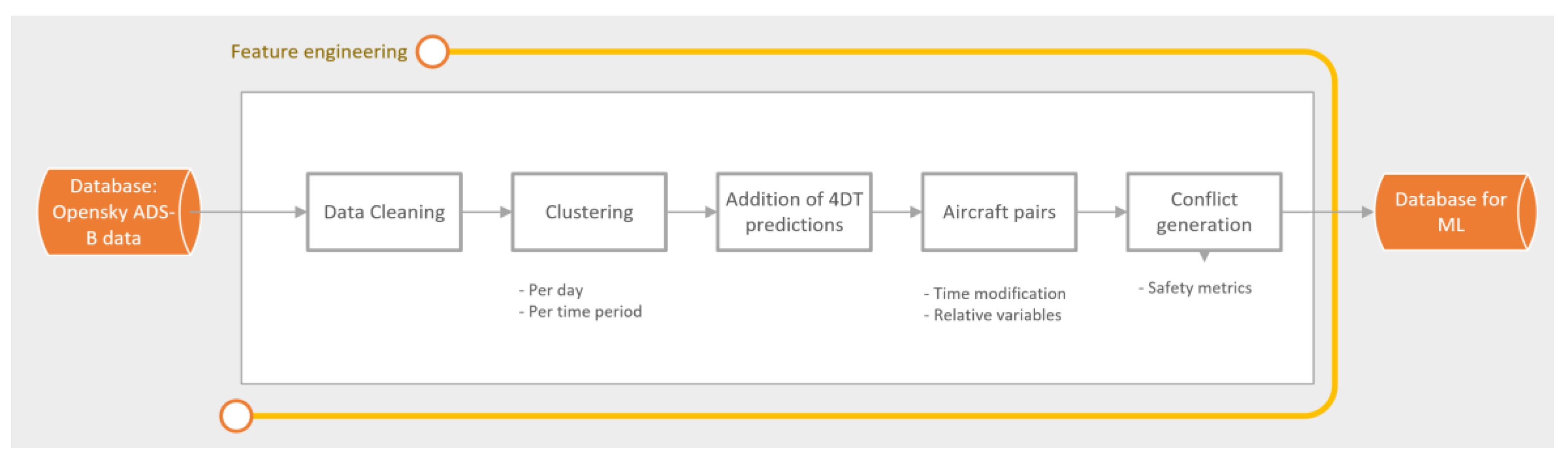
This work uses ADS-B trajectories from the OpenSky Network [33]. Raw data downloaded from the OpenSky network cannot be fed immediately to the ML algorithm. ML algorithms require previous filtering and adjustment to be used. Data preparation performs the following actions:

-

Cleaning trajectories that present errors in the ADS-B data. Errors in the ADS-B data are identified by the OpenSky functions [33] and represent faulty data such as callsigns or repeated positions. Trajectories with more than 10 ADS-B errors are removed. Duplicate trajectories are also removed.

-

Trajectories are gathered for each day and time period. One operational day is split into nine time periods based on the traffic distribution throughout the operational day. The first period covers from 0 to 8 a.m., and the traffic is removed because the LSAZM567 is not opened (due to the low traffic); the rest of the time periods are sets of two hours, and assume similar weather conditions in the simulations.

-

The generation of aircraft pairs based on the combinatorial problem.

-

Relative variables that combine operational features for each aircraft pair are calculated.

-

The generation of conflicts between aircraft pairs and the calculation of conflict metrics.

Figure 2 summarises the whole process.

Weather or operational variables of airspace status were not considered, and should be included in further work.

2.4. Historial ADS-B Database as 4DT Predictions

The operational concept considers 4DT predictions of the aircraft trajectories as inputs for the ML models. Each aircraft provides a trajectory prediction from the most basic information (the flight plan) until a 4DT prediction is calculated by the ground system. It was not possible to obtain this type of prediction because there was no access to the ground server or flight plans correlated with the ADS-B data. Therefore, the 4DT predictions were assumed to be historical trajectories stored from ADS-B data. It was assumed that the 4DT prediction can match with a similar trajectory stored in the ADS-B database. In case the system has another type of prediction, the process will be the same.

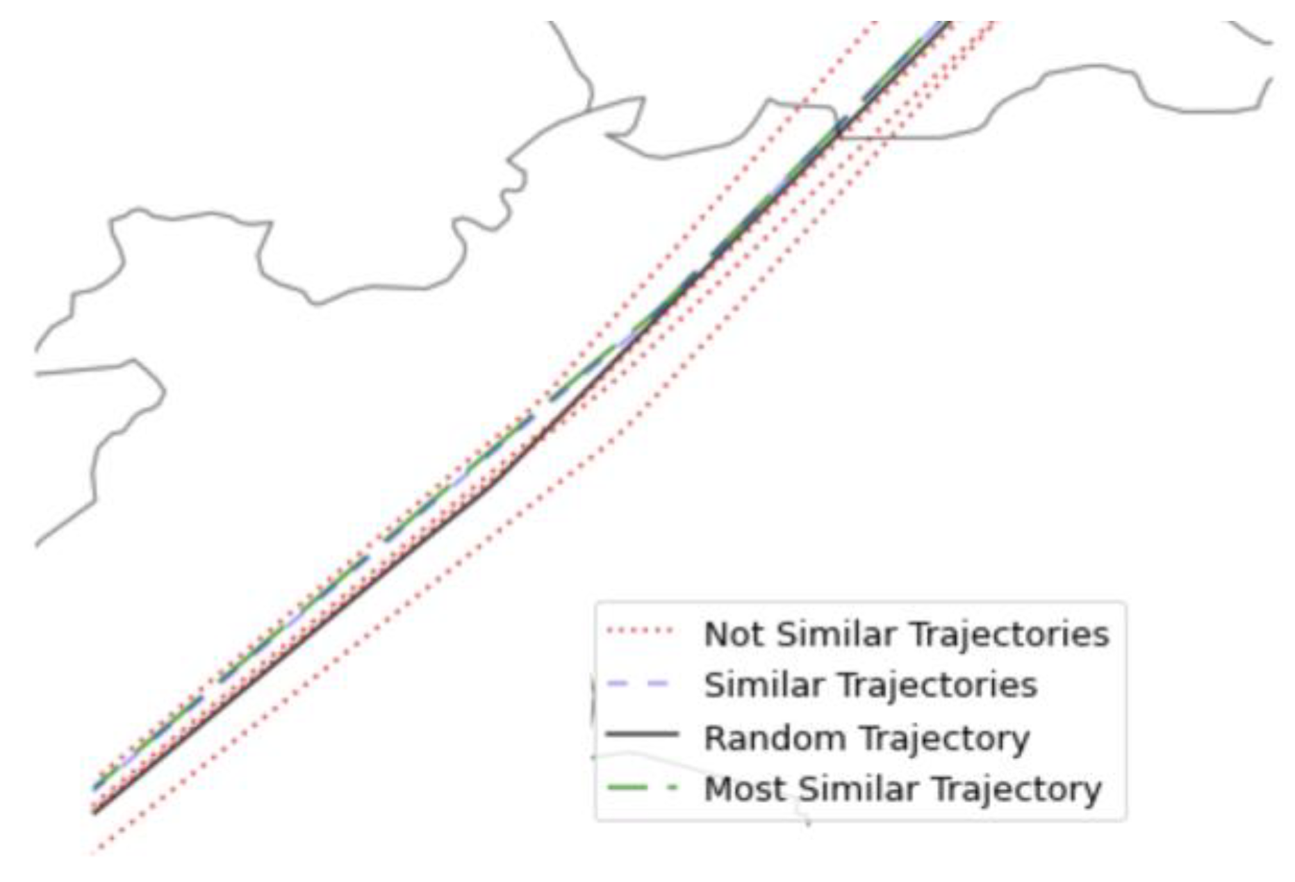
The main problem of using stored trajectories as 4DT predictions of other aircraft is ensuring the similarity between them. When one aircraft pierces into the airspace, the algorithm performs a search in the historical database in order to identify the most suitable trajectory that fulfils the following requirements:

• The first filtering is about selecting one trajectory with the same callsign. Typically, aircraft repeat their trajectories.
• The second filtering considers operational restrictions such as the ground speed, heading, and location of the entry point:

  ○

  The GS difference must be lower than 10 knots.

  ○

  The heading difference must be lower than 2°.

  ○

  The location difference of the entry points must be lower than 5 NM.

• In case there is more than one trajectory that fulfils the previous restrictions, it will select the trajectory with a lower heading difference.
• If none of the trajectories with the same callsign satisfy the previous restrictions or there are no trajectories with the same callsign, the algorithm extends the search to other callsigns. The main issue is that the computational time to find a similar trajectory increases exponentially.

Figure 3 represents the selection of a 4DT prediction from the historical database that is the most similar to one random trajectory when the aircraft pierces into the airspace.

Once the 4DT prediction is selected from the ADS-B database, two modifications are made to ease the interoperability. The first modification is about a resample of the 4DT prediction to reduce the number of samples that constitute the prediction. The goal of the resample is to reduce the computational workload and the size of the final database to consider due to the high number of samples. The resample is not an issue in the case where the aircraft fly straight lines, but if the aircraft is turning or performing a manoeuvre, it will not be reflected correctly.

The second modification aims to introduce uncertainty by adapting the 4DT prediction entry time to the actual trajectory. This uncertainty is a temporal deviation ($\tau$) following a random distribution of $\pm 20$ s. This is a value selected by the authors, and its suitability should be studied in further work. The higher this value, the larger the error between the actual trajectory and the 4DT prediction. The result is a database of 4DT trajectories composed of the actual trajectory and a similar trajectory considered as the 4DT prediction.

2.5. Generation of the Aircraft Pairs and Conflicts

The main limitation of the analysis of aircraft pairs extracted from ADS-B data is the lack of conflicts in real situations. Separation infringements safely occur in rare situations and under specific circumstances [34]. Conversely to these rare situations, ML models need a large and diverse database in order to learn the patterns that underlie separation infringement. Therefore, the first need is to generate a database with sufficient samples of conflict situations.

There are two ways to simulate conflicts. First, we can define the conflict parameters and then simulate backwards in order to obtain the conflicts which were previously defined. However, this solution does not encompass some operational parameters, such as airspace design or air traffic distribution. The second solution considers a real scenario and introduces modifications to the real trajectories in order to force separation infringements. These simulated conflicts are not real conflicts, but represent situations that could occur. These can be assumed to be pre-tactical conflicts based on real trajectories that consider many operational parameters, such as airspace design, speed uncertainty, and wind, etc. This work adopts the second approach and performs simulations that modify the entry time of the aircraft in a limited time period. In this way, an algorithm was developed to generate conflict situations by modifying their entry time. The process is as follows:

(1)

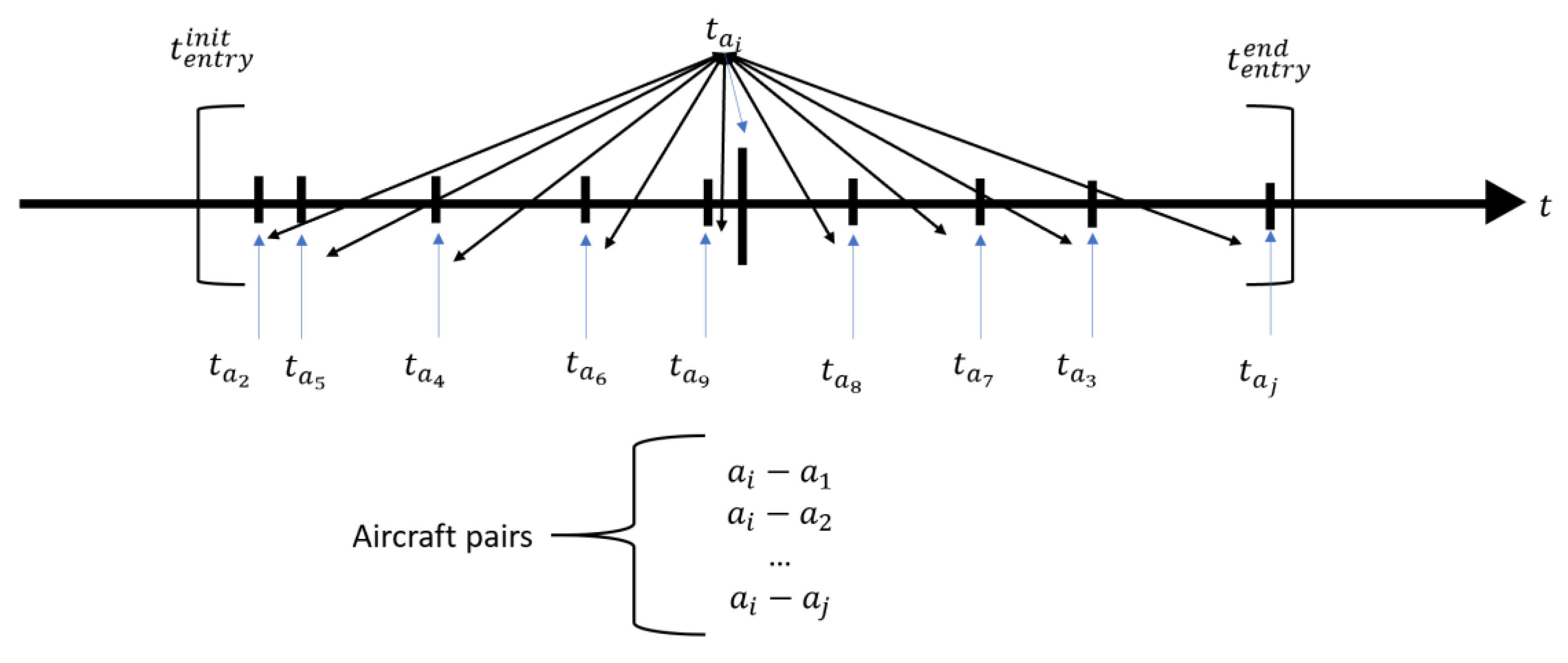
First, each aircraft modifies its entry time randomly between the temporary boundaries ($t_{entry}^{init}, t_{entry}^{end}$). The temporary restriction is that every aircraft should be in the airspace between the limits $t_{entry}^{init}$ and $t_{entry}^{end}$. The new entry times are calculated randomly for each aircraft.

(2)

Secondly, the aircraft pair generation is constituted. Suppose that there is a set of $n$ trajectories that constitutes $\left(n-1\right)n$ aircraft pairs. For each aircraft $i$ is generated an $\left(n-1\right)$ aircraft pair to evaluate.

(3)

For each aircraft pair at each time $t$, the database is constituted by storing the operational features of each aircraft pair.

(4)

Relative variables and conflict metrics are calculated for each aircraft pair, both for the actual trajectory and the 4DT prediction. Conflicts when one aircraft pierces into the airspace are discarded because this would imply that the ATCo from the previous airspace would not have done his work correctly.

Figure 4 represents this temporary modification and the generation of pairs for aircraft $i$. Aircraft $i$ pierces at time $t_{a_i}$, and the rest of aircraft receives aleatory new entry times between the time boundaries. The constitution of the aircraft pairs is repeated for every aircraft, avoiding duplicity.

Relative variables provide information about any situation that combines the operational features of a pair of aircraft. Relative variables are calculated at each timestamp when operational information is available. The mathematical descriptions of the relative variables are as follows:

• Horizontal separation ($s_{i,j}\left(t\right)$) is the horizontal separation between the locations of an aircraft pair:

  $$s_{i,j}\left(t\right)=positio{n}_i\left(t\right)-positio{n}_j\left(t\right)$$

  (3)
• Vertical separation ($\Delta h_{i,j}$) is the altitude variation ($h_i, h_j$) between an aircraft pair:

  $$\Delta h_{i,j}\left(t\right)=h_i\left(t\right)-h_j\left(t\right)$$

  (4)
• Course (${\gamma }_{i,j}$) is the course that links the locations between an aircraft pair:

  $${\gamma }_{i,j}\left(t\right)={\gamma }_i\left(t\right)-{\gamma }_j\left(t\right)$$

  (5)
• Track variation ($\Delta {\theta }_{i,j}$) is the track variation (${\theta }_i, {\theta }_j$) between an aircraft pair:

  $$\Delta {\theta }_{i,j}\left(t\right)={\theta }_i\left(t\right)-{\theta }_j\left(t\right)$$

  (6)
• Ground Speed ($GS$) variation ($\Delta G{S}_{i,j}$): is the difference in the module of the GS ($G{S}_i, G{S}_j$) between an aircraft pair:

  $$\Delta G{S}_{i,j}\left(t\right)=\left|G{S}_i\left(t\right)-G{S}_j\left(t\right)\right|=\sqrt{{\left(G{S}_i^x-G{S}_j^x\right)}^2+{\left(G{S}_i^y-G{S}_j^y\right)}^2 }$$

  (7)
• Vertical rate variation ($\Delta \dot{h_{i,j}}$) is the variation of the vertical rate ($\dot{h_i},\dot{h_j}$) between an aircraft pair.

  $$\Delta \dot{h_{i,j}}\left(t\right)=\dot{h_i}\left(t\right)-\dot{h_j}\left(t\right)$$

  (8)

The library geographiclib was used to calculate the relative variables based on aircraft positioning (longitude and latitude) because the library performs the calculations without transforming the aircraft positioning to Cartesian coordinates [35]. Therefore, 40 variables constitute the ML database: 12 ADS-B variables (six for each aircraft), six relative variables, two labels, and the same for the 4DT prediction.

2.6. Database for ML

The above process allows the performance of simulations to generate a database that could be used for ML models. The ML database presents situations of aircraft pairs that could constitute $SI$ or not.

This work was developed by the AISA project, and focused on the LSAZM567 sector of the Switzerland airspace (from FL355 to FL660) [36]. LSAZM567 airspace is an en-route airspace where most of the airways are composed of straight lines. The 4DT were downloaded from the AIRAC cycle from 20 June 2019 to 04 July 2019 (15 days). Approximately 12,500 trajectories were downloaded, containing more than 7e6 samples (each sample represents an aircraft position).

Table 1. Results of the simulations.

Variables	Number
Number of Aircraft	12,549
Number of pairs generated	1,257,234
Number of samples considered	675,3283
Samples with $SI$ (%)	1,215,152 (18%)
Samples with conflict (%)	270,132 (4%)
Computational time (hours)	420

shows the results for all of the simulations.

The number of aircraft varied from 80 to 120 for a one-hour period. The number of pairs generated was far from the whole combinatorial number of aircraft pairs because the simulations were performed for specific time periods. The total computational time required to perform the simulations was more than 420 h. This shows one of the issues that should be improved in future developments. Lastly, the simulations were performed in computer with Intel^® Core™ i5-6600 CPU @ 3.30 GHz, RAM 8.00 GB, and 64 bits.

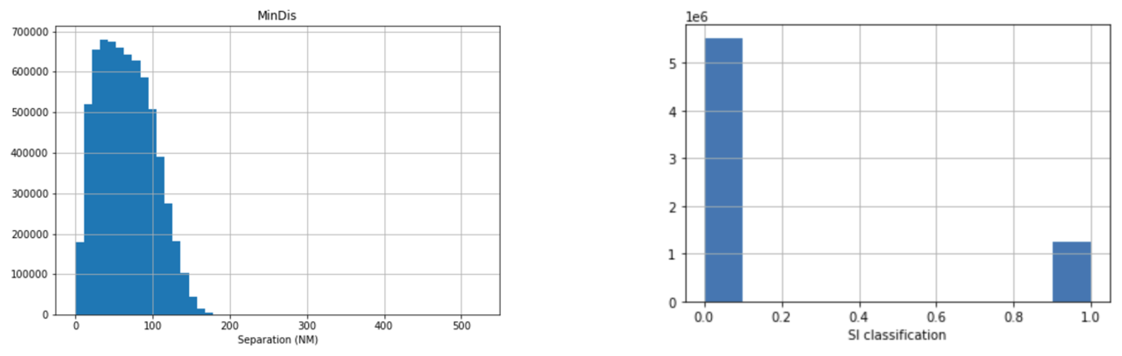
Figure 5 shows the histograms of the regression and classification targets.

As is shown in Figure 5, the $MinDis$ range of the distribution is from zero to more than 150 NM. The most significant density is between 10 and 20 NM. The $MinDis$ located at 0 NM refers to aircraft pairs that move away. Regarding the classification, there is a high imbalance between the $SI$ and $No SI$ samples and conflict samples. These results show the problem of generating conflicts despite using specific simulations for this purpose.

3. Machine Learning Techniques

One of the current technological developments is the implementation of data-driven techniques, and particularly ML, which is one of the most promising technologies in data prediction. As explained above, this approach tackles two types of ML problems: classification and regression. The classification problem aims to classify aircraft pairs into $SI$ or $No SI$ depending on the minimum separation that they are expected to reach. The regression problem seeks to predict the numerical value of the minimum separation they are expected to reach. It is important to note that both problems are solved independently. This allows one to analyse the validity of the combinations based on both predictions.

ML models are currently implemented in different programming languages. This work was developed in Python^®. Scikit-learn is the library which was used to implement ML algorithms [37], and PyCaret is another library that eases this process [38].

3.1. ML Experiments

As the ML database shows, there is a high imbalance between the $SI$ and $No SI$ samples. This is an issue in classification problems because the ML algorithm performs best with balanced databases. In order to tackle this problem, we considered a Hybrid model in which a filtering process based on operational restrictions was introduced to reduce the strong imbalance of the dataset. Then, there are two experiments:

• Pure model: The ML model considers the whole database without any modification.
• Hybrid model: The ML model considers a previously filtered database. The filtering is performed on the basis of operational restrictions. The database only contains aircraft pairs that cross with a horizontal separation of less than 20 NM and a vertical separation of less than 1000 ft.

The ML process performs the following steps to obtain the best ML model:

• The analysis of different ML algorithms: The first step is to evaluate the performance of different ML algorithms in order to identify the ML model that provides better results. In total, 15 ML algorithms were assessed for classification and regression.
• Feature selection: The feature selection identifies the influence of the different features that build the database, and analyses how they affect the model. The feature selection is performed based on graphical analysis and Recursive Feature Elimination (RFE) with CV [39]. RFE analysis evaluates the impact of the features on the model accuracy. Finally, features without influence on the ML model are removed from the database.
• ML optimisation: The optimisation process aims to improve the algorithm’s performance based on a grid search of the hyperparameters. The hyperparameters must be set up in advance of the training model, and can be defined as the settings of an algorithm. The metric to be optimised depends on the classification and regression problem.

The result of this process is the readiness of two trained and tested ML algorithms for conflict detection.

3.2. ML Database Preparation

The ML process requires the preparation of the database prior to feeding it to the algorithms. Data preparation modifies the raw data into valuable data for ML algorithms. Here, the following preprocessing activities are applied:

-

The training and testing sets: The dataset is divided into the training and testing datasets. The testing set (also known as the hold-out set) works as a proxy for new data. It is not used in model training, and can be used to evaluate the model metrics’ suitability. The database is split into 70% for training and 30% for the testing set.

-

Normalisation: Normalisation rescales the values of the numeric columns following a normal distribution. It does not distort the differences in the range of values.

-

Shuffling: This distributes the samples randomly into the training and testing datasets.

-

Stratification: Apart from randomly distributing the samples, the stratification process spreads the samples whilst maintaining the $SI$ statistical distribution.

-

Cross-validation: This is a process which is used to avoid the overfitting of the ML model [39]. The training set is divided into k folds: one is considered the validation set, and the rest are considered the training set. This process is repeated for every k-fold, and the metrics are calculated based on the mean and standard deviation.

Table 2. Number of samples for each experiment and set.

Model	Training Set	Testing Set
Pure model (18/82)	4,254,567	1,823,387
Hybrid model (68/32)	1,140,470	488,773

shows the number of samples for both experiments; the rates of $SI/No SI$ samples appear in parentheses. Each sample represents the situation of one aircraft pair at one specific time.

3.3. ML Algorithms and Metrics

Currently, there are several state-of-the-art ML algorithms, and we evaluate some of them. The evaluation of different algorithms allows one to identify the best among them. The goal of this section is not to explain the algorithms employed, but to denote which were trained: Extra Trees, Random Forest, Extreme Gradient Boosting, Light Gradient Boosting, CatBoost, Decision Tree, K Neighbors, Gradient Boosting, Ada Boost, Naïve Bayes, SVM—Linear Kernel, Logistic Regression, Ridge Classifier, Linear Discriminant Analysis, and Quadratic Discriminant Analysis. The authors encourage readers interested in the mathematical ML definitions to see [20]. Other ML techniques such as Deep Learning could improve the results, and should be evaluated in further work.

ML metrics are different for classification and regression problems:

-

Classification problems include accuracy, precision, recall and F1. The most important is the F1 metric that leverages precision and recall. Accuracy is not a good option because the database is highly imbalanced.

-

Regression problems include the Mean Absolute Error (MAE), Root Mean Square Error (RMSE), R2 and Root Mean Square Logarithmic Error (RMSLE). The most important metric is the RMSE, which increases the impact of the prediction distance from the true values.

4. Results

This section provides the results of the experiments, and are split into classification and regression. In addition, the performance of both predictors is analysed for different separation infringement stretches.

4.1. ML Techniques for Classification

ML classification techniques predict whether an aircraft pair is $SI$ or not. The first step is to analyse the performance of different ML algorithms, aiming to identify the best one. The results of the different ML algorithms are shown in ‘Appendix A ML results’ in order to improve the reading of the paper. Both experiments agree that the three top algorithms vary between Extra Trees, Random Forest and Decision Tree, i.e., ensemble models. The random forest provided the best results for both experiments. The models were evaluated on the basis of stratified cross-validation techniques in order to avoid overfitting.

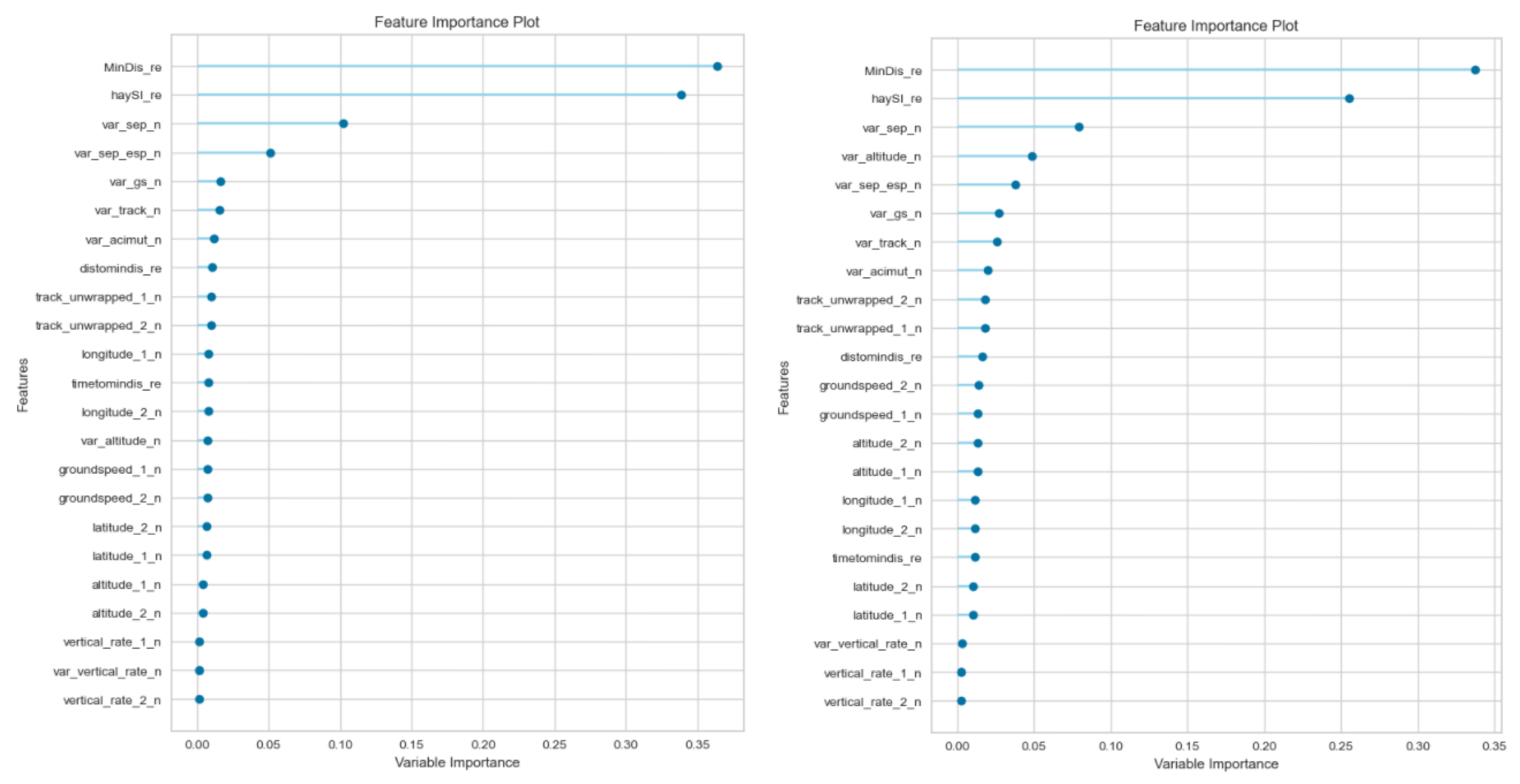
The feature selection for both experiments concluded that the most influential features were the prediction about the minimum distance and the $SI$ prediction. The sum of both of them reached around 70% of the influence of the variable. The variation of separation is also important (up to 10%), and the rest of the features provide a similar impact between 1 and 5%. As can be seen in Figure 6, the feature selection is similar for both experiments (Pure and Hybrid models). This similarity confirms the significance of the prediction variables in the ML algorithm. The variables labelled ‘_n’ refer to the aircraft trajectory, and ‘_re’ refers to the 4DT prediction.

The next step is to optimise the Random Forest algorithm. The database is imbalanced in both experiments because the distribution of $SI$ samples is not balanced. This issue is tackled by implementing cost-sensitive techniques during the optimisation process. We studied the optimisation of recall, precision and F1. However, the most balanced results were obtained by optimising the F1 metric.

Table 3. Results of the classification experiments.

Experiment	Accuracy (std)	Recall (std)	Precision (std)	F1 (std)
Pure model	0.990 (0.01)	0.987 (0.01)	0.989 (0.02)	0.988 (0.01)
Hybrid model	0.991 (0.001)	0.990 (0.001)	0.991(0.001)	0.990 (0.002)

shows the results of both experiments in the training set applying a fivefold cross-validation.

The following conclusions were obtained:

-

The optimisation process barely improved the initial metrics of the ensemble models. The initial values obtained for the ensemble models were very high, and the improvements obtained by optimising the hyperparameters were reduced by up to 1%. This implies that identifying the correct model is crucial because the subsequent optimisation process does not provide substantial gains.

-

The metrics of both models were extremely high and similar; their rates were almost 99% for every metric. Although the Hybrid model provides better metrics than the Pure model, the difference was less than 2%. This implies that the usage of unbalanced datasets does not greatly affect classification purposes by implementing cost-sensitive techniques.

These results confirm the goal of this research on the introduction of ML techniques. Therefore, ML algorithms learn from the initial prediction and improve the quality of conflict prediction.

4.2. ML Techniques for Regression

ML regression techniques predict the numerical value of the minimum separation to be reached by an aircraft pair. The first step is to analyse the performance of different ML algorithms, aiming to identify the best one. The results of the different ML algorithms are shown in ‘Appendix A ML results’ in order to improve the reading of the paper. Both experiments agree that the three top algorithms vary between Extreme Gradient, Light Gradient and Gradient Boosting, i.e., ensemble models. Extreme Gradient provides the best results for both experiments. The models were evaluated based on stratified cross-validation techniques in order to avoid overfitting the results.

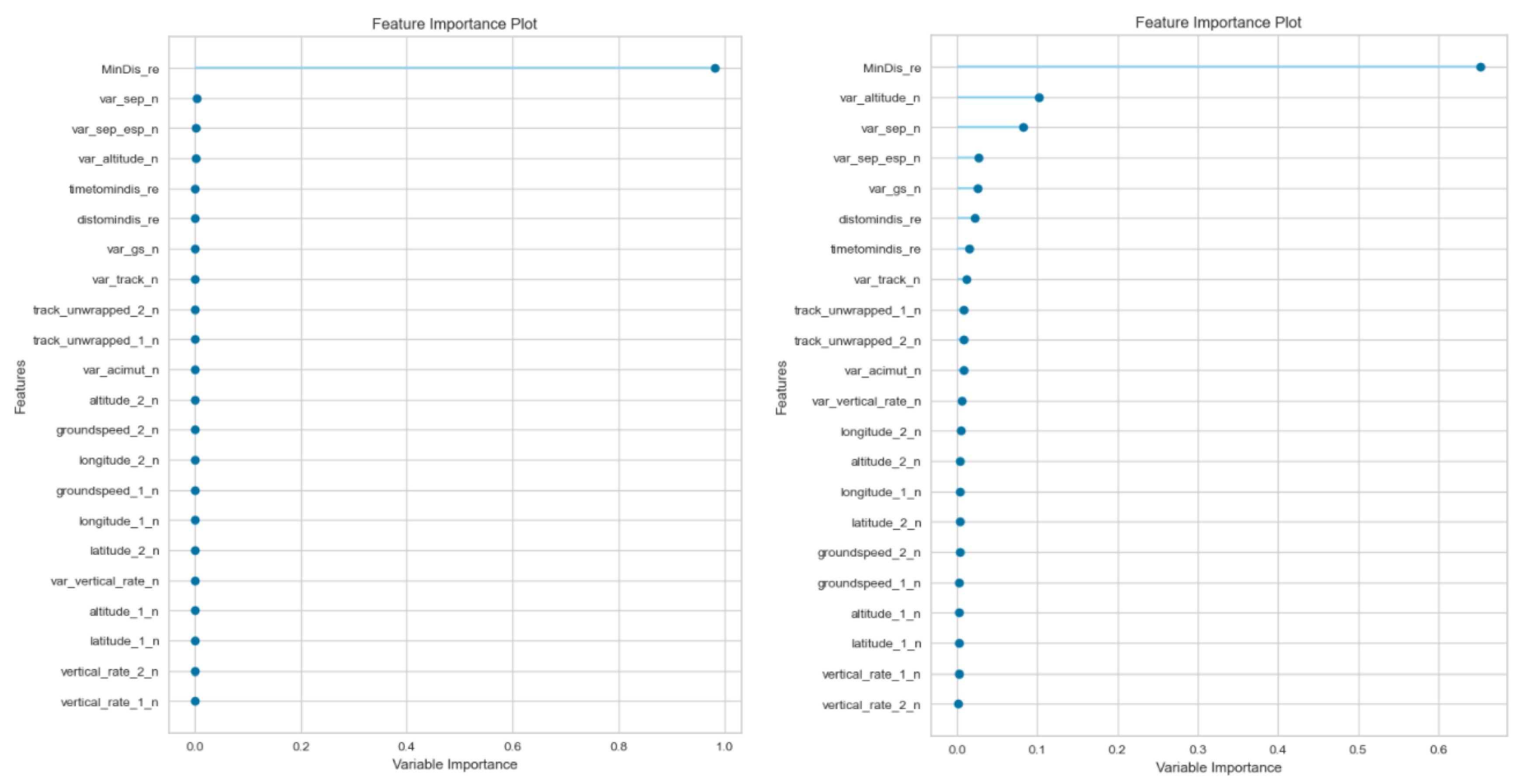
Both experiments concluded that the most influential feature is the prediction of the minimum distance. However, the influence varied from the Hybrid model (over 60%) to the Pure model (almost 100%). The rest of the variables provided influence values lower than 1% for the Pure model; as such, the Pure model was analysed without them. However, the Hybrid model requires more variables, such as the variation of the altitude and the horizontal separation among others. Figure 7 shows these results and does not confirm the similarity identified in the feature importance of the classification experiment. In addition, the analysis shows a performance decrease of more than 2%, which does not recommend removing the features.

The next step is to optimise the Extreme Gradient algorithm. Only the optimisation of RMSE was studied.

Table 4. Results (NM) of the regression experiments.

Experiment	RMSE	MAE	R2	RMSLE
Pure model	2.579	1.601	0.994	0.178
Hybrid model	1.473	0.992	0.934	0.235

shows the results of both experiments on the training set applying a fivefold cross-validation.

The following conclusions were obtained:

-

The optimisation process improves the initial metrics by up to 10% in some experiments. This implies that the behaviour of the Extreme Gradient model greatly depends on the optimisation process, conversely to the random forest during the classification optimisation.

-

The results differed between the Pure and Hybrid models. The best results were obtained for the Hybrid model (1.5 NM). The Pure model worsens the RMSE over 1 NM, which implies an increase of over 40% compared to the Hybrid model.

-

These results are different from the classification problem because cost-sensitive techniques cannot be applied to the Pure model. The higher imbalance of the Pure dataset means a clear decrease in the metrics of the regression predictors.

4.3. Analysis of ML Technique Prediction

This section analyses the performance of the predictions of the ML techniques between them in the testing set. The goal is to identify which predictions the ML models (classification and regression) tend to fail or guess right and match. Therefore, the predictions of both models will be compared considering only the Hybrid model that provided the best results. The predictions are split into four ranges in order to differentiate between $SI$ and conflict.

Table 5. Distribution of the classification and regression predictions.

Experiments	$\mathit{M}\mathit{i}\mathit{n}\mathit{D}\mathit{i}\mathit{s}\_\mathit{M}\mathit{L}$ = (0,5]	$\mathit{M}\mathit{i}\mathit{n}\mathit{D}\mathit{i}\mathit{s}\_\mathit{M}\mathit{L}$ = (5,10]	$\mathit{M}\mathit{i}\mathit{n}\mathit{D}\mathit{i}\mathit{s}\_\mathit{M}\mathit{L}$ = (10,15]	$\mathit{M}\mathit{i}\mathit{n}\mathit{D}\mathit{i}\mathit{s}\_\mathit{M}\mathit{L}$ = (15,20]
$SI\_ML$ = 1	100%	97%	18%	0%
$SI\_ML$ = 0	0%	3%	82%	100%

shows the allocation of the classification and regression predictions in the four ranges. The analysis concludes that the predictions fail at the 10 NM border. In case both ML predictors confirm a conflict, the conflict probability is 100%. In opposition, the probability is 100% when both predictors discard an $SI$. However, the samples with a predicted value of 10 to 15 NM only guess 82% right. The samples with a predicted value from 5 to 10 NM guess 97% right. It can be concluded that the model only fails in the classification when the predicted value of $MinDis$ is between 5 and 15 NM, especially if it is between 10 and 15 NM.

Table 6. Distribution of the classification predictions and real values.

Experiments	$\mathit{M}\mathit{i}\mathit{n}\mathit{D}\mathit{i}\mathit{s}\_\mathit{R}\mathit{e}\mathit{a}\mathit{l}$ = (0,5]	$\mathit{M}\mathit{i}\mathit{n}\mathit{D}\mathit{i}\mathit{s}\_\mathit{R}\mathit{e}\mathit{a}\mathit{l}$ = (5,10]	$\mathit{M}\mathit{i}\mathit{n}\mathit{D}\mathit{i}\mathit{s}\_\mathit{R}\mathit{e}\mathit{a}\mathit{l}$ = (10,15]	$\mathit{M}\mathit{i}\mathit{n}\mathit{D}\mathit{i}\mathit{s}\_\mathit{R}\mathit{e}\mathit{a}\mathit{l}$ = (15,20]
$SI\_ML$ = 1	100%	91%	6%	5%
$SI\_ML$ = 0	0%	9%	94%	95%

makes the same comparison between the classification predictions and the real values of the samples.

Although the values are quite similar, there are some differences compared to Table 5:

• The percentages of correctly classified samples between 0 and 5 NM are the same (100%). These results confirm that training the model using $SI$ instead of conflict provides a 100% guess of conflict.
• The model predictions fail at the 10 NM limit. The predictions from 5 to 15 NM present higher misclassification errors. However, when we use both predictions (classification and regression), the misclassification errors decrease from 5 to 10 NM by increasing the false rate from 10 to 15 NM.

The errors considered from 5 to 10 NM are samples considered from 10 to 15 NM; these errors do not impact the aircraft pairs classified as $SI$.

5. Conclusions

This article develops the pillars for the further development of an ATC tool based on ML techniques. This work is framed on a Technology Readiness Level 1–2 based on the European project to which it belongs. It was developed in order to analyse the viability of introducing ML techniques for conflict detection purposes by analysing their accuracy and expected errors. The introduction of ML techniques in safety-critical areas in air traffic management is very complex, and must be properly analysed in order to ensure the feasibility of these techniques. This paper develops a data-driven approach that considers the evolution of the aircraft within the airspace, and the separation evaluation along with it. The trajectories were extracted from the OpenSky Network based on ADS-B information. One of the difficulties was the generation of conflict. One limitation of using real ADS-B trajectories is that the trajectories that suffered a tactical modification by the ATC action could not be removed.

Real ADS-B trajectories were temporarily modified, considering specific aircraft sets in the same time period, to constitute the $SI$. In addition, historical ADS-B trajectories were used for 4DT predictions as inputs for the ML models. The introduction of 4DT predictions as an input is crucial in order to obtain such high metrics. One of the strong points of this approach is the use of real ADS-B trajectories to constitute the database. Using real trajectories means that this work could be developed for real scenarios. Moreover, the introduction of 4DT trajectories presents a twofold implication: (1) it shows the clear improvement provided by introducing this information, and (2) this methodology could be developed for other types of predictions (such as pretactical trajectories from the Network Manager or calculated by the ATC ground system).

The results confirmed that ML models can be applied to perform conflict prediction. The best algorithms for both problems are the ensemble methods. Notably, Random Forest for classification and Extreme Gradient for regression provided the best results in the experiments. The main problem is the large dataset used to train the models, which demanded substantial computational time and computer resources. Classification techniques reach a success rate of more than 99% for $SI$ prediction and regression techniques up to 1.5 NM in RMSE. In addition, both ML models were identified to have ensured 100% success in conflict detection (a separation infringement lower than 5 NM) combining both predictions. These results confirm the appropriateness of using 10 NM as the boundary to train the model instead of 5 NM.

Finally, this work brings to light the possibility of introducing ML techniques for conflict detection purposes, although it deals with some limitations in different areas due to its novelty. Further work should focus on: (1) the introduction of Deep Learning based on neural networks, (2) the introduction of operational and environmental variables not considered herein, and (3) the introduction of other sources for 4DT predictions as an input.