Abstract
In this paper, the design and validation of a heat storage device based on phase change materials are presented, with the focus on improving the thermal control of micro-satellites. The main objective of the development is to provide a system that is able to keep electronics within safe temperature ranges during the operation of manoeuvres, while reducing mass and volume in comparison to other thermal control techniques. Due to the low thermal conductivity of phase change materials, the conductivity of the device as a whole is one of the major challenges of the development. This issue has been solved by means of the use of a lattice of aluminium fins. The thermal behaviour of the proposed solution is assessed with numerical simulation tools, and the results prove that the developed phase change material-based thermal control technique is able to provide the suitable integrated thermal management of micro-satellites. Fabrication challenges found in the project are also explained. Numerical results are validated through a testing stage. The predicted temperature profiles are in good agreement with experimental data and inside the range foreseen for the heat storage device.
1. Introduction
Space is a very harsh and difficult environment for spacecraft and their payloads. From a thermal point of view, spacecraft and payloads must undergo extreme temperatures, heat fluxes and variations in these flows depending on the orbit type [1,2].
Thermal control refers to the set of techniques employed to maintain the temperatures of the spacecraft and its components inside the range of allowed temperatures [3,4]. This must be achieved in all possible scenarios (hot cases, cold cases, steady state or transient cases, etc.) because, otherwise, individual components can fail due to the very high or very low temperatures reached. A failure in one component, e.g., the electronics, can jeopardize a mission or even make it a failure [5].
Phase change materials (PCM) have been used for thermal control techniques since the early years of the 1960s. Several Apollo missions carried components that used PCMs to stabilize their temperatures [6]. Other components were also used that relied on PCM behaviors [7]. The general appreciation in the space industry for PCMs continued also during the 21st century, as was shown by the call from the European Space Agency (ESA) to the European space industries to design, calculate and fabricate a phase change material heat storage device (PCM-HSD) [8].
The physics and behavior of PCM materials have been widely studied in the literature [9,10,11,12,13,14,15,16,17,18,19,20]. One interesting study showed the possibility of using PCMs to stabilize the temperature of some components, for instance, the electronics [1]. When the different electronic circuits are switched on, heat is produced, and temperatures start to rise. The heat produced must be conducted to the radiator and, from there, must be evacuated into outer space. If the power to be disposed of is big, the surface of the radiator must also be big and, consequently, its weight will be high. However, if the power produced by the electronics is somehow ‘stored’ in the PCM, and the temperature is maintained at a constant level, it will be possible to dispose of the heat when the circuits are switched off. This means that the area of the radiator will not be that large, the weight will be lower and the design will be better. In fact, what the PCM achieves is an increase in the thermal inertia of the spacecraft or payload and, in this way, it will have a more stable temperature and a reduced weight of the payload or spacecraft.
2. Phase Change Material Heat Storage Device (PCM-HSD)
2.1. Description
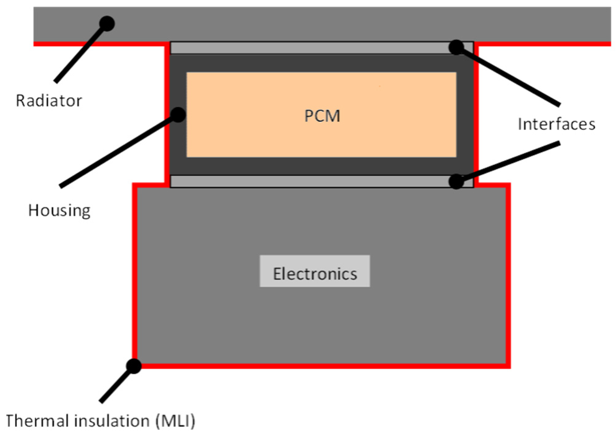
This study aimed to assess the possibility of using PCMs in space to stabilize the temperatures of components and to reduce the size of the radiator in order to reduce weight. The system considered, shown in Figure 1, was based on a PCM contained in a house, which was attached to the electronics whose temperature is to be controlled and the radiator. Every surface but the radiator was assumed to be covered by multi-layer insulation (MLI) blankets to avoid heat leaks. Moreover, the radiator was assumed to operate just when the heat needed to be released into the space. The device was considered, therefore, to be insulated from the environment to make the study conditions more unfavorable.

Figure 1.
Phase change material heat storage device (PCM-HSD) considered.
The key idea behind this PCM thermal control concept is to convert the thermal energy into a phase change reaction, storing heat when it is produced and releasing this energy when the electronics is switched off. Since the phase change process occurs at almost constant temperature, such thermal control means that the system temperature does not change significantly during the melting/solidification, so that if the melting point is appropriate, the electronics can be efficiently protected.
In general terms, micro-satellites (between 10 and 100 kg in weight) operate on low Earth circular orbits (LEO, 450–1200 km) with a wide range of NASA β angles, and on high elliptical orbits, and are exposed to the Sun, albedo and infrared Earth radiation. Typical maximal incident fluxes for 550 km orbit for flat surfaces with normal to nadir trajectories are QIR (infrared) ~200 W/m2 and QAL (albedo) max ~450 W/m2 (averaged over orbit <150 W/m2). The eclipse time can vary between 0.5 h (circular) and up to several hours for elliptic orbits. According to Baturkin [21], typical requirements of average heat generation inside the satellite are in the range of 15–40 W. This power is produced mainly by housekeeping equipment (on board computer, transmitter, the attitude and control system, batteries). Peak heat generation coincides with payload operation and can reach up to 200 W.
In our case, the specifications that were to be followed are those stated by the ESA [8]. There were requirements for functional and performance (FPR), interface (IR), environmental (ER), operational (OR), design (DR) and verification and testing (VTR) operations. However, the main requirements are those related with thermal capacity and mechanical behavior, listed below:
- The device must be capable of absorbing 30 W for 45 min;
- Operational temperature range must be (−20/+40 °C);
- The device’s mass shall be less than 0.50 kg;
- The device’s first resonance frequency must be higher than 140 Hz;
- The device shall sustain a mechanical environment characterized by dynamic loads.
2.2. Governing Equations and Numerical Methods
It is very common for thermal control in spacecraft to describe the heat transfer process through the thermal lumped method (TLP). Details about the method can be found elsewhere [22,23,24].
The set of nonlinear equations that describe the temperatures of a transient thermal mathematical model is (for a node )
where is the number of nodes of the thermal mathematical model (TMM), is the conductive conductance (W/m) between nodes and , is the Stefan–Boltzmann constant (5.67 × 10 − 8 W/(m2·K4)), is the radiative conductance (m2) between nodes and , and are the temperatures (K) of nodes and , is the product of the node mass (kg) times the heat capacity (J/(kg·K) and is the power (W) that enters into node . The subscripts and go from 1 to . It is usual to ascribe thermal inertia to the product as it describes the “opposition” to changing the temperature of node when subjected to a power input.
The time derivative of the temperature of node can be approximated by
For a node and for a general time step , it is possible to write
In order to simplify the notation, the following will be used
Additionally, the following set of equations is obtained
Each equation represents the thermal instant equilibrium of a node. An in-house-developed computer program called TK was used to solve the set of non-linear equations. These equations are solved for each time step where temperatures of the different nodes are calculated. The heat power (W) that goes from one node to another is also calculated, as well as the heat power (W) that goes into each node, which is employed in increasing its temperature. The TK computer program was modified to be able to deal with phase change materials. In the following, we will assume that the initial state of each node is solid and that the phase change will be melting.
For those nodes made of PCMs, additional information must be supplied to the computer program. The PCM has a latent heat , measured in J/kg. The mass of each node (kg), as well as the specific heat (J/(kg·K)) of the material are also known. By multiplying the mass of the node by the latent heat , the program can obtain the total energy needed by the node when passing from a solid to liquid phase.
The program uses a predictor–corrector method to take into account the latent heat of nodes made of PCM. For each time step, a set of temperatures is calculated (predicted) with the previously explained equations. Then, the program checks each node made of PCM. If the temperature predicted for this node is higher than the starting temperature of the change of state from solid to liquid, then the energy used (J) is calculated, the temperature of the node is corrected and the accumulated energy used in that node is calculated, as is the liquid fraction of PCM in that node. These calculations are performed taking into account the product of the mass times the specific heat of the node. If the calculated liquid fraction is lower than 1, the program continues with the next node. When the total energy accumulated in one node is higher than the total energy that the node needs to change state, the state of the node is considered liquid and, in the following time steps, it will not have influence over the predicted temperatures.
It is clear that time steps short enough must be considered when phase change takes place, otherwise significant errors can appear. It is not unusual to need to make several trials before fixing an appropriate time step length. Finally, the procedure for considering the change from liquid to solid is similar, but with decreasing temperatures.
3. Design of the Phase Change Material Heat Storage Device (PCM-HSD)
3.1. Conceptual Design
The design efforts are aimed at creating an appropriate heat management technique to keep the electronics within the safe temperature range and a suitable housing design able to withstand the structural loads specified. Together with the specifications mentioned in the previous section, the main issues considered for the conceptual design were the PCM selection and the PCM thermal conductivity enhancement. It has not been previously mentioned but, in general, thermal conductivity of PCMs is quite low, and it is necessary to improve it to obtain an appropriate thermal behavior for the device.
3.1.1. PCM Selection
Regarding the PCM selection, a first calculation has been performed to find the minimum value of the latent heat needed for the PCM. Following the specifications, Equation (6) states:
In fact, the minimum value for the latent heat of the PCM must be bigger, because the PCM will be positioned inside a container that will add mass to the device but almost no latent heat (not taking into account the specific heat).
A box-shaped aluminum container with a, b, c dimensions and t thickness has been considered. Aluminum has very good thermal conductivity and a relatively low density, so as a first approximation, it has been selected as the container material. Values for dimensions a and b have also been selected as 80 mm and 20 mm, respectively. The reason is that these dimensions are adequate for one of the mechanical interfaces considered. A thickness of t equal to 2 mm has also been selected because of the fabrication constraints, so the only unknown dimension left is the height c. It is possible to demonstrate that the c maximum value (in meters) that can be accepted for the box if the maximum weight of the PCM-HSD has to be 0.5 kg must be
where and are the densities of the container and the PCM.
Once the general dimensions of the PCM-HSD are known, it is possible to calculate the energy that the PCM-HSD can handle due to the latent heat for a particular PCM. If this energy is higher than 81 kJ (162 kJ/kg 0.5 kg), it is possible to conclude that the selected PCM is appropriate for the application.
Several organic and inorganic PCMs have been studied, and the first selection criterion has been that the energy calculated with Equation (2) is bigger than 81 kJ. In addition, the good chemical compatibility between the PCM and the structural material has been considered.
3.1.2. Enhancement of the Thermal Conductivity
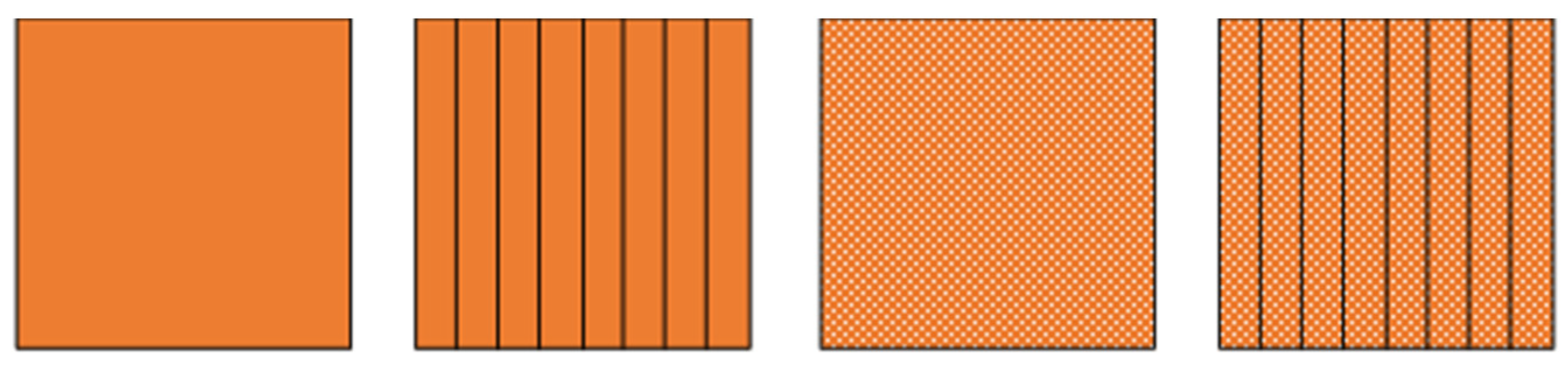
As it has already been mentioned, the thermal conductivity of the PCMs is, in general, low. This can pose a problem for the PCM-HSD because higher than desired temperatures could be reached while the phase change occurs, endangering the functioning of the electronics. In this context, an introductory calculation has been performed, comparing the behavior of the PCM alone with its behavior if aluminum fins are present, if aluminum foam is used or if even both of them, fins and foam, are used simultaneously (Figure 2). The calculation is based on the mixture rule and gave an initial idea of what to expect from each solution.
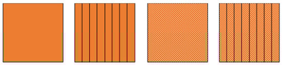
Figure 2.
From left to right, PCM, PCM with fins, PCM with foam, PCM with fins and foam.
To calculate the equivalent thermal conductivity, we have taken into account the conductivity of the PCM, the conductivity of the fins and also the transversal area of the fins. In the foam case, the apparent conductivity has been considered, which is a function of the material conductivity and the pore density:
performing some algebra in Equation (3), it is possible to write:
where:
: PCM-HSD equivalent thermal conductivity (W/(m·K));
: The phase change material’s thermal conductivity (W/(m·K));
: The fins’ thermal conductivity (W/(m·K));
: The real foam’s thermal conductivity (W/(m·K));
: The apparent foam’s thermal conductivity (W/(m·K));
: The transversal area of the PCM (m2);
: The transversal area of the fins (m2);
: The transversal area of the foam (m2);
: The apparent density of the foam (kg/m3);
: The real density of the foam (kg/m3).
For this preliminary analysis, a paraffin called RT5HC was selected as the PCM (properties in Table 1), with a metallic foam Duocel® (Table 2) and aluminum alloy 6101 for the fins (Table 3).

Table 1.
PCM RT5HC material properties (supplier: Rubitherm).
Table 2.
Duocel® foam material properties.
Table 3.
Aluminum material properties.
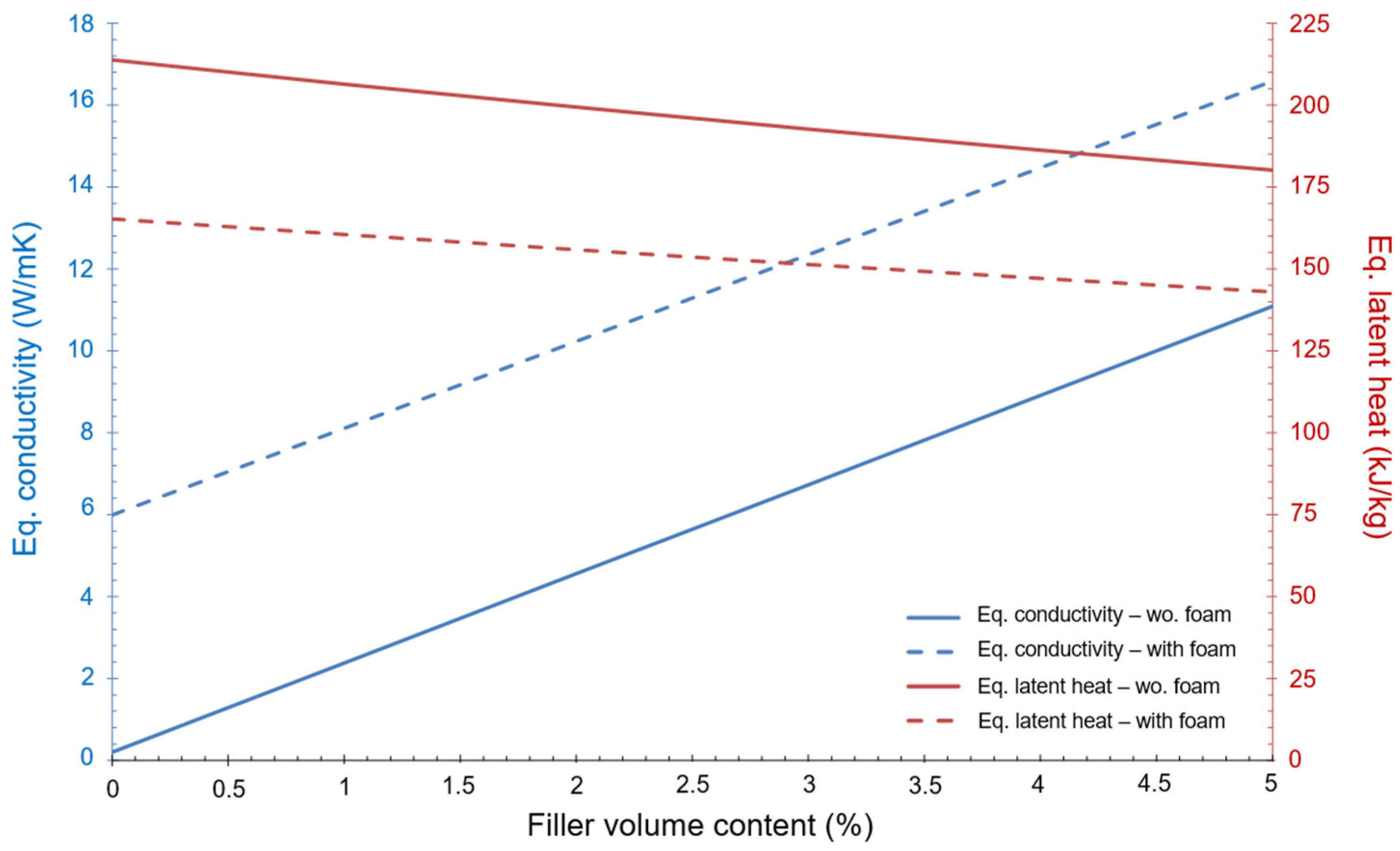
It is worth to noting that the PCM (RT5HC) selected for this first approximation does not fulfil the condition imposed regarding the minimum energy (i.e., be higher than 81 kJ). However, the purpose of this initial investigation is to estimate the variation of the equivalent conductivity in relation to the percentage of filler volume content. This variation, as well as the equivalent latent heat, can be seen in Figure 3. The dot lines express the values when foam is present, as well as the fins. The continuous lines show values with only fins.
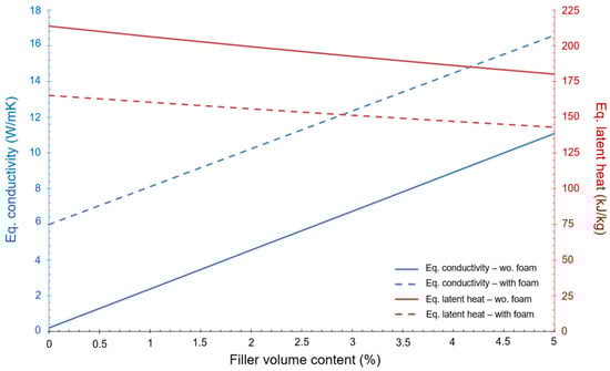
Figure 3.
Variation of equivalent conductivity and equivalent latent heat as a function of the % of filler volume content.
Figure 3 shows that the equivalent conductivity of the device improves a lot when foam and fins are present but, at the same time, the equivalent latent heat of the device decreases significantly. The final design should be a trade-off between these two aspects of the heat transfer mechanism.
3.1.3. Initial Conceptual Design
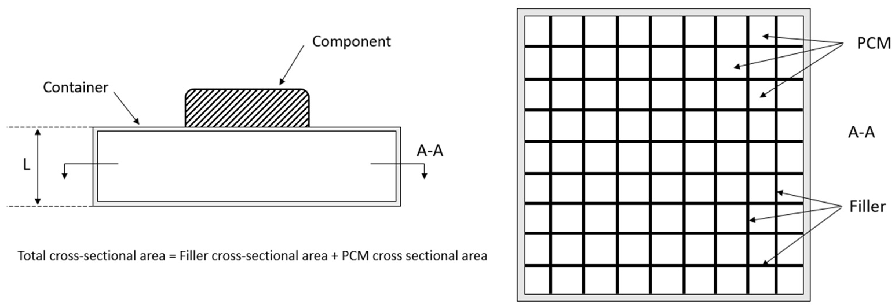
Reference [1] provides a good method for the geometrical initial design of the PCM-HSD. Assuming a geometry similar to the one shown in Figure 4, a spreadsheet has been prepared to evaluate different initial designs in a quick and efficient way.
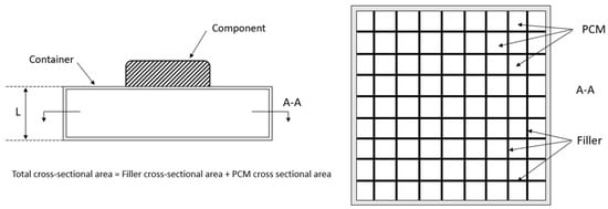
Figure 4.
Initial basic design of the PCM-HSD.
The basic equations taken into account are the energy conservation, Fourier’s law, the mixture rule and mass conservation. The inputs for the spreadsheet are the PCM properties, general dimensions of the housing, number and thickness of the fins and their properties and the properties of the foam. The obtained results are the total mass of the device (maximum 0.5 kg), the thermal energy that can be dealt with (minimum 81 kJ) and the equivalent thermal conductivity.
It can be seen that the device’s weight is 0.5 kg and that the total energy is 87.9 kJ: both constraints are then fulfilled.
3.2. Preliminary Design of Two Possible Phase Change Material Heat Storage Devices
The process of elaborating a new design is, without a doubt, an iterative process that only converges when the final design is built. In our case, two preliminary designs, based on two phase change materials (RT5HC and KF·4H2O), have been developed. The geometries are quite different, and both designs needed to be calculated thermally and mechanically. For the sake of completeness, the material properties of both materials are collected in Table 4.
Table 4.
Material properties for the preselected phase change materials.
Both materials comply with the ESA specifications previously mentioned. Perhaps the most relevant point of interest of the KF·4H2O salt is that it undergoes almost no change in volume when melting.
3.2.1. RT5HC Material
The proposed design for this material can be seen in Figure 5. The previously mentioned spreadsheet was used, with some minor adaptations.
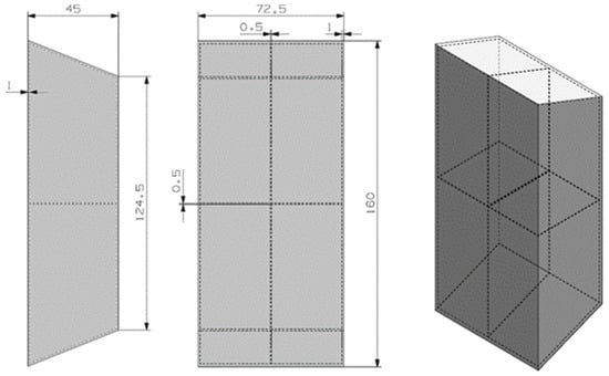
Figure 5.
Preliminary design for the RT5HC material.
The trapezoidal geometry tries to maximize the surface contact between the hot electronic device and the PCM material. The design has two inner fins to improve the thermal conductivity of the device. The container material is the 6101 aluminum material.
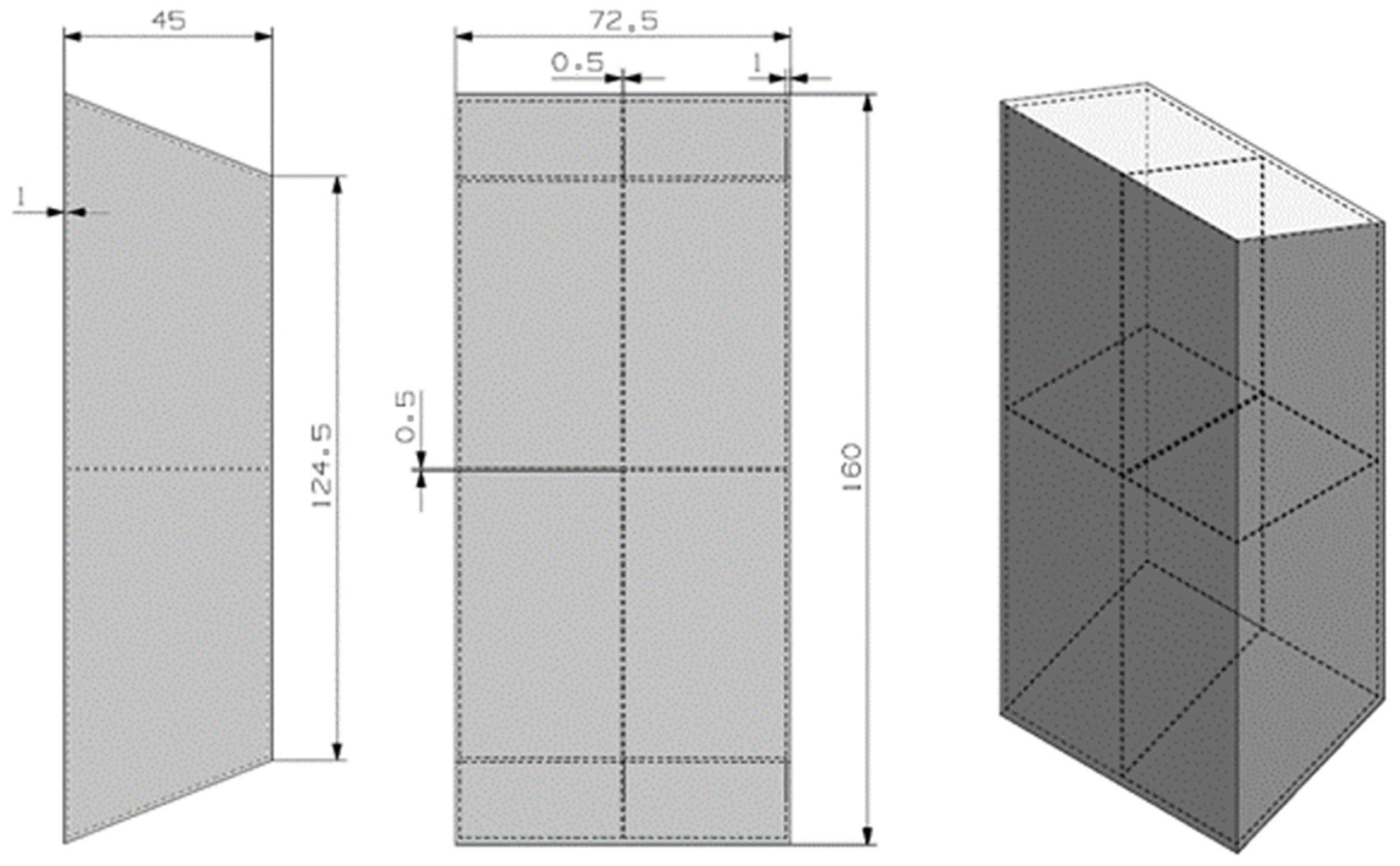
3.2.2. KF·4H2O Material
A fairly different preliminary design was depicted for the hydrated salt material, see Figure 6. The design was conceived to take advantage of the almost-constant density of the PCM material for solid and liquid phases. The number of inner fins is bigger in this case, again to improve the thermal conductivity. The material container is again 6101 aluminum material, and the estimated weight is 0.5 kg.
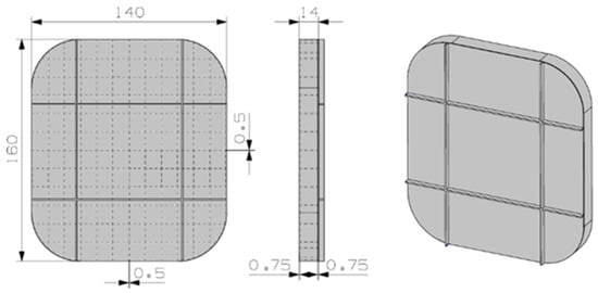
Figure 6.
Preliminary design for the KF·4H2O material.
3.3. Detailed Design: Thermal and Mechanical Modelling of the Phase Change Material Heat Storage Devices
The preliminary designs proposed in the previous section of the paper must undergo a detailed thermal and mechanical analysis before being fabricated. This is performed in order to check whether the designs fulfill the requirements expressed in Section 2.
3.3.1. Thermal Behavior Modelling
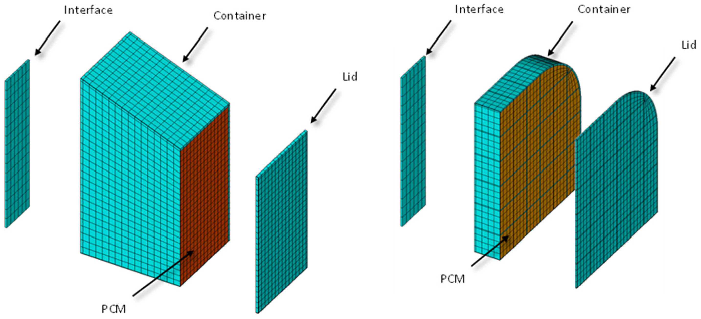
The commercial thermal software NX-TMG from Siemens has been used for the transient calculation of the system temperatures. The employed mesh can be seen in Figure 7.

Figure 7.
Detailed mesh employed in the thermal calculation.
The NX TMG software automatically converts the finite element mesh shown in Figure 7 into a network of thermal conductance values employed in the thermal lumped parameter (TLP) method, which is very well known in the space industry [24]. Thermal resistances have been added manually to the models to take into account the contact between the interface and the PCM container. The employed value is 0.070 × 10⁻⁴ m2K/W, taken from [25]. The mesh represents a quarter of the real geometry due to the symmetry presence. Both thermal interfaces (small and big) have been modelled for completeness of the calculations. The objective is to maintain the temperature between −20 °C and +40 °C.
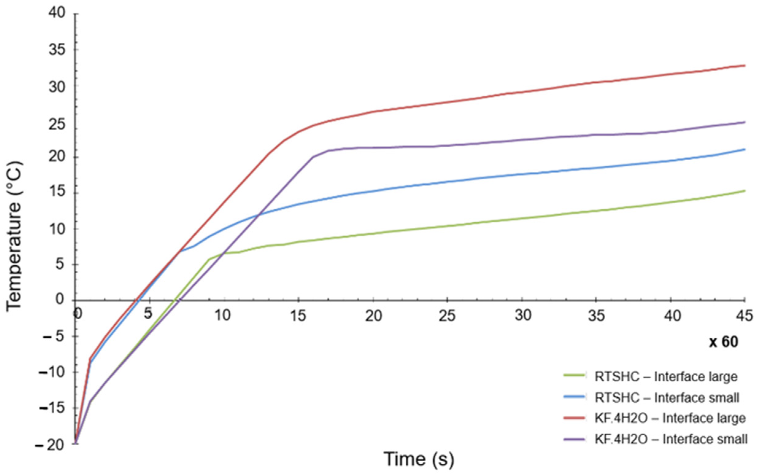
The thermal load case applied in each of the four geometries is a heat flow of 30 W produced by the electronics, applied for 45 min. The initial temperature considered is −20 °C and a time step of 0.1 s was used, which makes a total of 27,000 steps. The results for the most critical point of the PCM-HSD (a point in the interface, near the electronics) are shown in Figure 8.
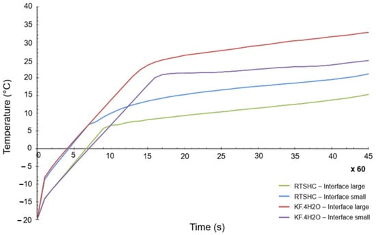
Figure 8.
Highest temperature of the PCM-HSD in a transient calculation.
As can be seen, even for the most critical point of the design, the maximum allowed temperature of 40 °C is not reached. It can be also concluded from Figure 8 that the small interface generates higher temperatures than the large one, as it would be expected.
3.3.2. Mechanical Behavior Modelling
Both static and dynamic loads are foreseen for the different mission phases where the PCM-HSD can be used. As a consequence, different load cases are analyzed.
Volume Change during the Phase Change
It is well known that volume change appears when the phase change occurs in the PCM materials. Different materials have different volume changes and, for the two preselected materials, the changes were estimated through Equation (11):
To simulate this increase in volume, hydrostatic pressure has been calculated and applied to the two containers previously described. For the RT5HC material, an equivalent load of 60 bars has been applied, and for the KF·4H2O, the applied hydrostatic pressure is 1.25 bars. As could be expected, the maximum stresses calculated with the finite element method are high at more than 1000 MPa (one thousand), and the maximum displacements around 8.8 mm in the case of the RT5HC. These levels of stresses and displacements are not possible, so the RT5HC material and its correspondent design were discarded.
The results are more encouraging for the KF·4H2O, as the maximum stresses present in the container are around 177 MPa, which is correct from a structural point of view. Figure 9 shows the equivalent von Mises stresses and the maximum displacements of this case. The employed mesh is similar to that of Figure 7.
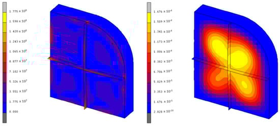
Figure 9.
Von Mises stresses (Pa) and displacements (m) of the KF·4H2O container.
Dynamic Response of the PCM Heat Storage Device
Three different requirements are present in the specification of the mechanical dynamic behavior of the PCM-HSD. NX CAE software was used for the following calculations:
- First natural frequency must be higher than 140 Hz. This requirement was analyzed through an FEM calculation. The first frequency calculated is above 1200 Hz, so the requirement is fulfilled. It is interesting to note that as the PCM is considered in its liquid phase for this calculation, a non-geometrical mass homogenously applied on the inner walls of the container has been used.
- Random forced dynamic response. The requirements are collected in Table 5. Results show an RMS acceleration of 215 g, which produces a maximum of 18 MPa, well inside the allowed range.
Table 5. Sinus and random force dynamic requirements.
- Sinus excitation. As stated in Table 5, the system must undergo a sinus excitation for frequencies between 5 and 1000 Hz of a 25 g level, with a sweep rate of 2 octaves/minute. As the first natural frequency is far enough from the excitation frequencies, the obtained von Mises stresses are quite low.
4. Fabrication of the Phase Change Material Heat Storage Devices
The fabrication of the PCM-HSD posed several challenges, and some final changes were made to the detailed design. It is important to remember that the design and fabrication of the PCM-HSD was a research project and allowed some flexibility, along as this was inside the requirements of the specification.
4.1. PCM Material
It was not possible to find a reliable supplier for the KF·4H2O hydrated salt. After much effort and lack of success, the working team decided to change the selected salt for another one called Glauber’s salt, Na2SO4·10H2O, whose commercial name is PlusICE S32. The material thermal properties are presented in Table 6.
Table 6.
Thermal properties of PlusICE S32.
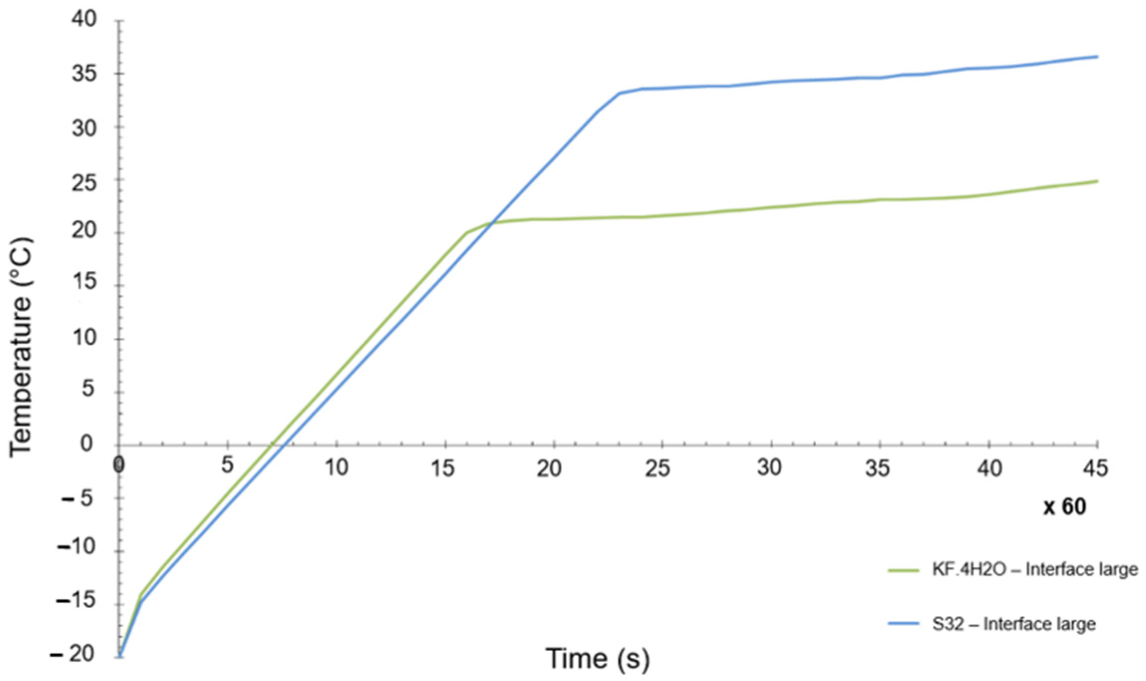
The objective was to have a PCM as close as possible to the original selection. In general terms, the differences between both materials were not that big, but there is one key difference, which is the melting temperature. Whereas the initial melting temperature of the KF·4H2O hydrated salt was 18.5 °C (see Table 4), the melting point of the Na2SO4·10H2O was 32 °C. A numerical transient simulation of the temperature reached can be seen in Figure 10. The final achieved temperature is around 37 °C, clearly higher than the one previously calculated, but within the acceptable range of values. However, the margins are now quite tight (the maximum allowed temperature is 40 °C).
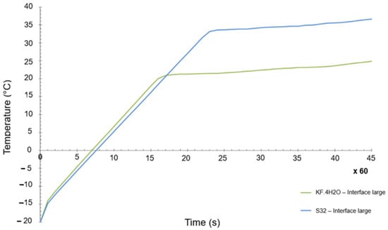
Figure 10.
Transient temperature evolution of KF·4H2O and S32 PCM materials.
4.2. Container Material
The change in the PCM material made it necessary to change also the container material, as it was compulsory to ensure the compatibility between the new PCM and the container [26]. The main point was that the new container should be Cu-free, so a 6063-T5 alloy was selected. The high thermal conductivity of the container was thus maintained, and strength properties are similar.
4.3. Container Fabrication Process
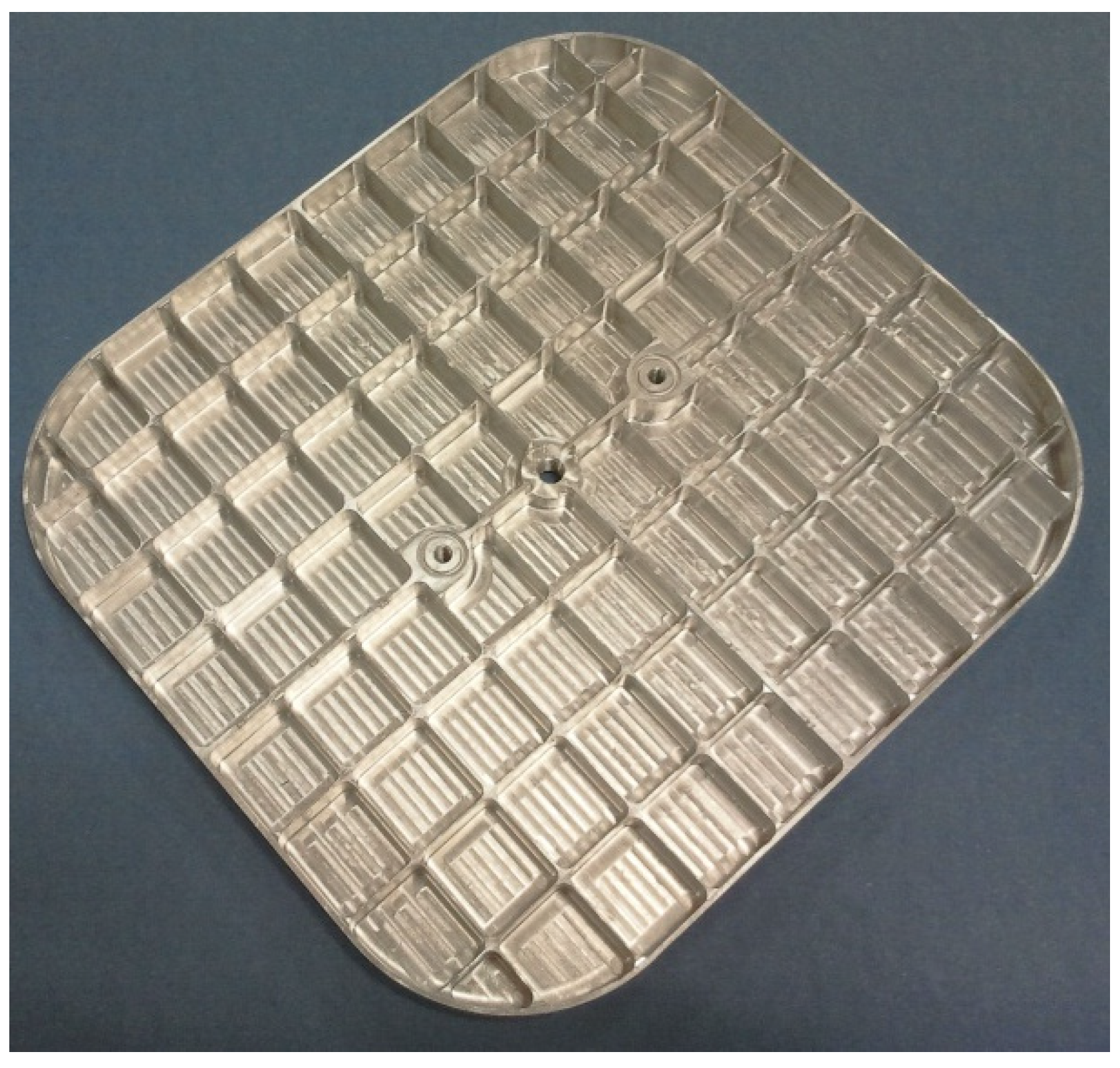
The fabrication process was also complex, as the geometry of the container is not simple. One of the main difficulties was the thickness of the walls (0.4 mm). Two fabrication processes were tested: electroerosion and machining. Both, after several trials, gave satisfactory results, so machining was selected due to budget considerations. Figure 11 shows the container base.

Figure 11.
Container 6063-T5 base.
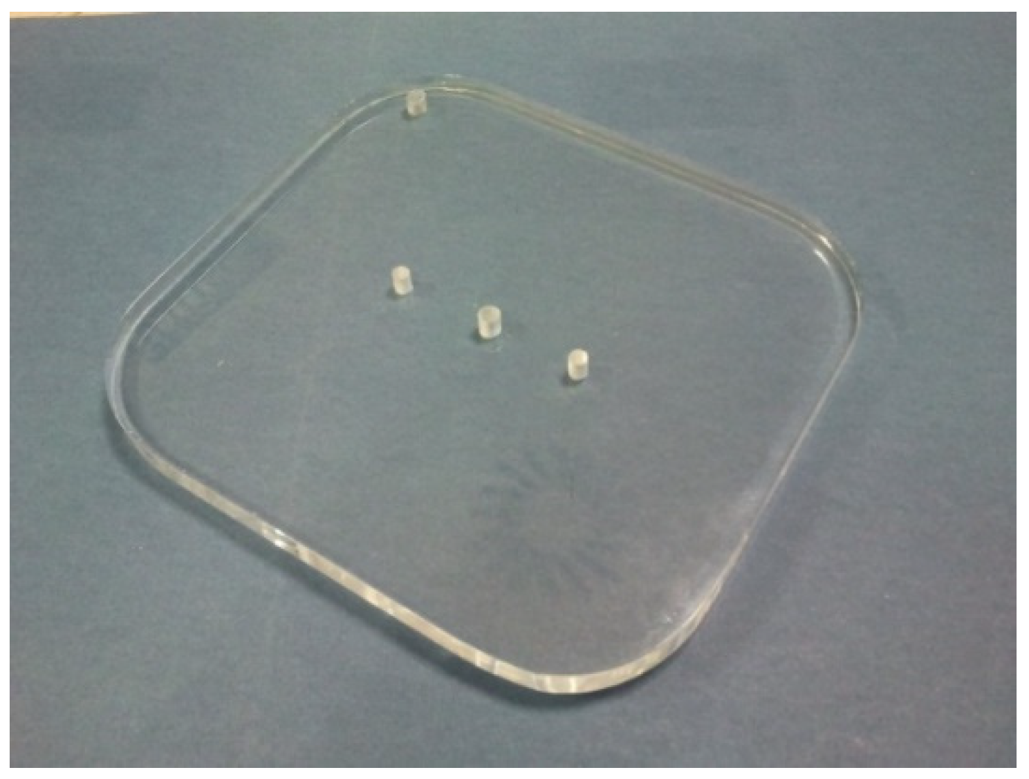
Finally, we decided to fabricate the container lid in methacrylate. The rationale behind this decision is the special interest of the working team in the change of phase of the PCM material. With this transparent material, it was going to be possible to see the process itself and see whether the assumptions adopted during the design process were correct. The thermal conductivity of the methacrylate is lower than the aluminum alloy, but it was considered to be good enough. The other drawback of the approach is that the dynamic tests will not be conducted, as the mechanical properties of the material are not equivalent to those of the 6063-T5 alloy. However, it was considered that the numerical tests conducted and explained in Section 5 of this paper were good enough for the purposes of the project. Figure 12 shows the final lid in methacrylate.
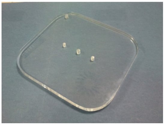
Figure 12.
Container methacrylate lid.
5. Testing and Experimental Validation
A testing stage was conducted in order to assess the thermal performance of the PCM-HSD system under realistic conditions and to validate the thermal models used. For the tests, the base and the lid were joined by means of two screws and sealed with o-rings. Additionally, Terostat MS-9399 elastic sealing was applied along the frame of the housing in order to avoid material leaks. The phase change material was injected in liquid phase, ensuring a suitable void volume after material solidification to allow the volume increase accommodation when melting the PCM without stressing the device.
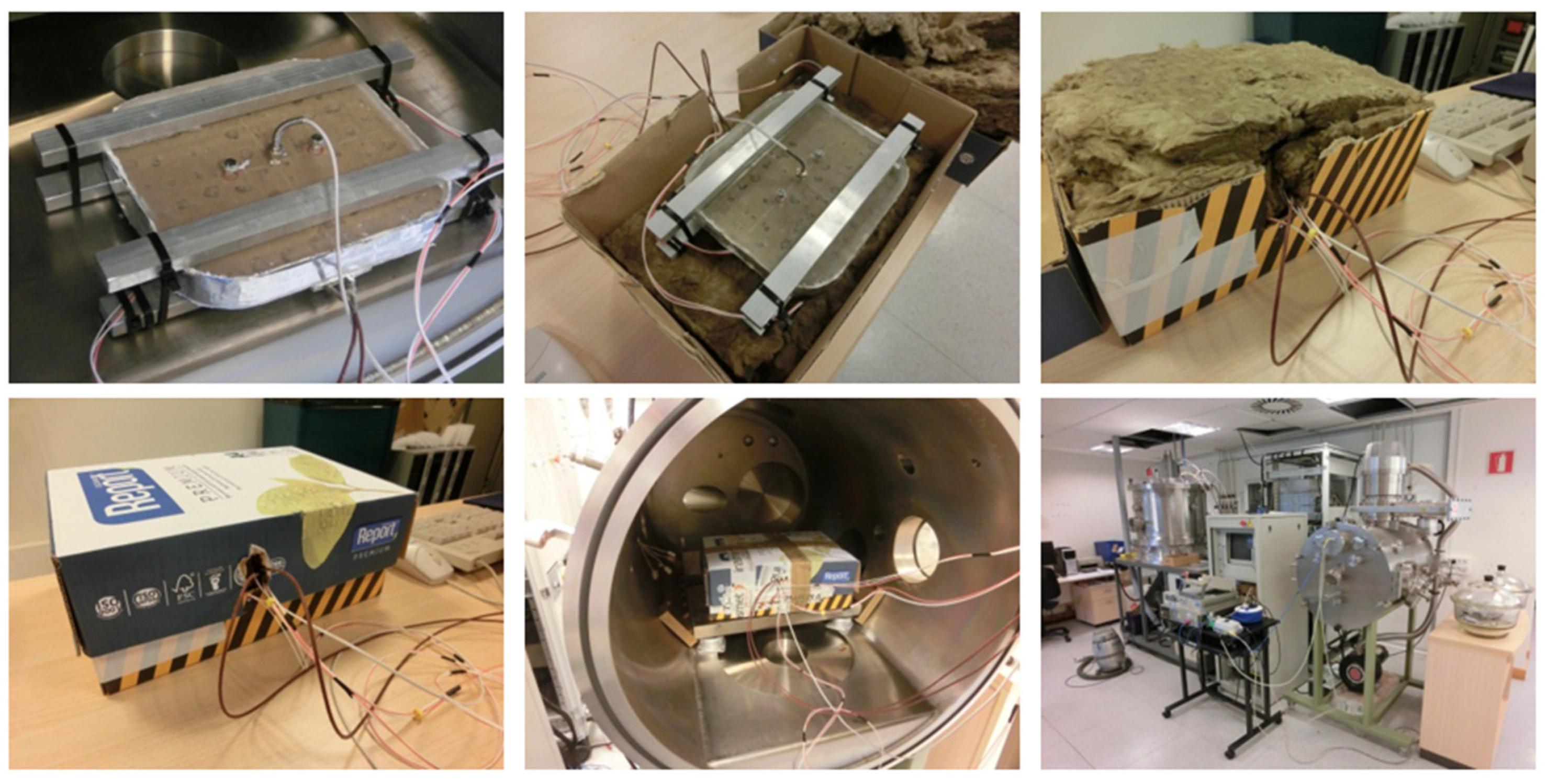
The testing stage was conducted with controlled vacuum conditions and power dissipation in a vacuum chamber. A vacuum of 5 × 10⁻⁶ bars was established. The initial temperature of the test was the ambient temperature. The electronics were simulated through a heater designed to fit the surface area and heat dissipation. To ensure a proper heat transfer from the heater to the device, a silicone heat transfer compound was applied in the interface and some pressure was exerted. The device was insulated with Alpharock E-225 40 mm from Rockwool to avoid heat leaks to the environment, and this was introduced in a box. Pictures of the testing device and equipment are presented in Figure 13.

Figure 13.
Pictures of the testing device and equipment.
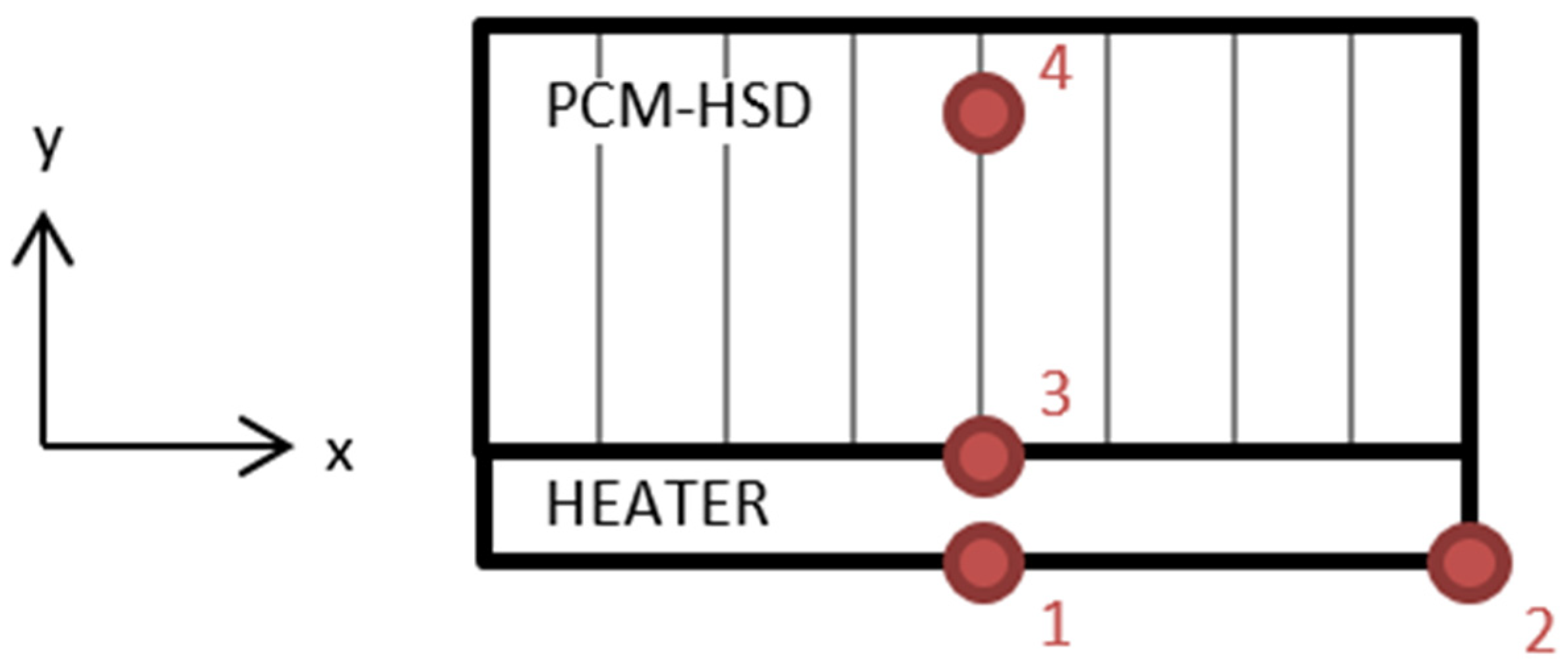
Four PT100 resistance temperature detectors (RTD) were placed for the temperature measurements, as shown in Figure 14.

Figure 14.
Location of the resistance temperature detectors.
Location 1 is on the center of the heater, location 2 is on one side of the heater, location 3 is in the heater–device interface and location 4 is inside the device, in contact with the PCM.
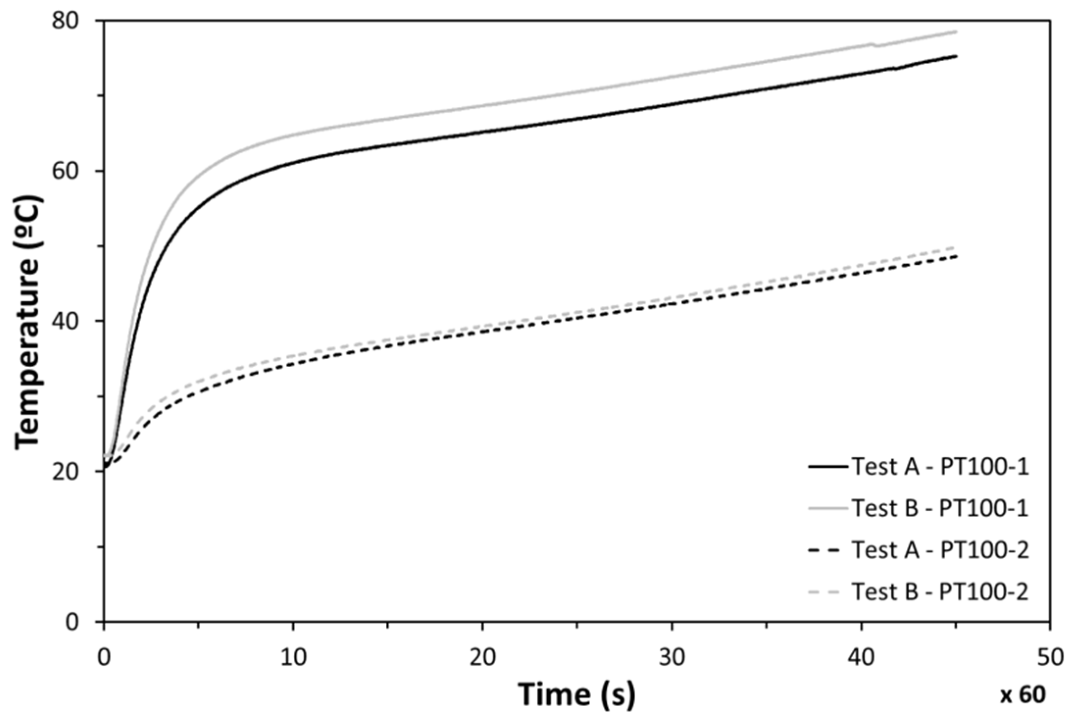
Good repeatability was found between experiments when the cycle of 45 min was followed under identical conditions. The temperature in the center of the heater (PT100-1) was found to be much higher than the measurements on the lateral side (PT100-2) (Figure 15). Those differences are caused by the fact that the incoming heat flux is not as uniform as expected. This non-uniformity makes the temperature in the center impractical to measure, while lateral measurements (PT100-2) were identified to be realistic for the electronics temperature evolution analysis.

Figure 15.
Temperatures at points 1 and 2 during tests.
The temperature evolution of PT100-2 and PT100-1 is presented in Figure 16, along with the results from the simulation. An excellent agreement was observed between the computer modelling and tests. Both the simulation and experimental results presented an initial quick temperature increase and a subsequent slope change caused by the melting process. Minor temperature deviations were observed between the numerical results and measurements during the whole heating process. Differences at the beginning were concluded to be related to the thermal inertia of the insulation materials used. Temperature deviations detected at the end were identified to be caused by the fact that the inserted PCM amount in the testing stage was slightly lower than the simulated one. On the basis of this correlation, the numerical models were validated, confirming that way the simulation results.

Figure 16.
Temperature evolution of the PCM-HSD.
6. Conclusions
In this work, a heat storage device based on PCMs was designed, manufactured and tested according to realistic specifications for micro-satellites. The developed device was formed of an aluminum housing filled by PlusICE S32 salt hydrate from EPS Ltd. Heat transfer limitations related to the low thermal conductivity of the phase change material were dealt with via the insertion of aluminum fins. A suitable design was reached considering weight restrictions, heat transfer and capacitance and mechanical requirements. Numerical analyses were carried out considering realistic load conditions and showed that the reached maximum temperature was within a safe range. The developed thermal control system was tested in specific laboratories, controlling vacuum conditions, power dissipation and boundary conditions. Experimental results showed an excellent agreement with simulations. The minor deviations detected were considered to be mainly related to the insulation materials, the PCM amount included in the device and the PCM thermal conductivity change from the solid to liquid phase. The performed activities proved that the device was able to absorb the heat flux incoming from the electronics of micro-satellites without exceeding in the electronics the upper limit.
Author Contributions
Conceptualization, methodology and investigation, H.V., M.S. and I.G.; writing, review and editing, I.G., H.V., E.A. and M.S.; project administration, M.S.; funding acquisition, I.G. and M.S. All authors have read and agreed to the published version of the manuscript.
Funding
This work was supported by the Spanish Ministry of Economy and Competitiveness through the financial support given to the project “Soluciones térmicas para componentes espaciales basadas en materiales con cambio de fase” (ref: AYA2010-18663).
Institutional Review Board Statement
Not applicable.
Informed Consent Statement
Not applicable.
Data Availability Statement
Not applicable.
Conflicts of Interest
The authors declare no conflict of interest.
References
- Gilmore, D.G. Spacecraft Thermal Control Handbook, 2nd ed.; Gilmore, D.G., Ed.; American Institute of Aeronautics and Astronautics: El Segundo, CA, USA, 2002; Volume 1, ISBN 1-884989-11-X. [Google Scholar]
- Silk, E.A. Introduction to Spacecraft Thermal Design; Cambridge University Press: Cambridge, UK, 2020. [Google Scholar]
- Meseguer, J.; Pérez-Grande, I.; Sanz-Andrés, A. Spacecraft Thermal Control; Woodhead Publishing: Cambridge, UK, 2012; ISBN 978-0-84569-996-3. [Google Scholar]
- Miao, J.; Zhong, Q.; Zhao, Q.; Zhao, X. Spacecraft Thermal Control Technologies; Springer: Singapore, 2021; ISBN 978-981-15-4983-0. [Google Scholar]
- Karam, R.D. Satellite Thermal Control for Systems Engineers; Progress in Astronautics and Aeronautics; Zarchan, P., Ed.; American Institute of Aeronautics and Astronautics: Reston, VA, USA, 1998; Volume 181, ISBN 1-56347-276-7. [Google Scholar]
- Morea, S.F. The Lunar Roving Vehicle: Historical Perspective. In Proceedings of the The Second Conference on Lunar Bases and Space Activities of the 21st Century, Houston, TX, USA, 5–7 April 1988. [Google Scholar]
- Keville, J. Development of Phase Change Systems and Flight Experience on an Operational Satellite. In Proceedings of the 11th Thermophysics Conference, San Diego, CA, USA, 14–16 July 1976; American Institute of Aeronautics and Astronautics: Reston, Virigina, 1976. [Google Scholar]
- European Space Agency. Statement of Work, “Phase Change Materials for Space Thermal Applications”, TEC-MTT/2010/2721/Ln/RPL, AO6477-Ws00pe; European Space Agency: Paris, France, 2010. [Google Scholar]
- Zalba, B.; Marín, J.M.; Cabeza, L.F.; Mehling, H. Review on Thermal Energy Storage with Phase Change: Materials, Heat Transfer Analysis and Applications. Appl. Therm. Eng. 2003, 23, 251–283. [Google Scholar] [CrossRef]
- Lane, G.A. Solar Heat Storage: Latent Heat Materials, Volume 1: Background and Scientific Principles; CRC Press: Boca Raton, FL, USA, 1983. [Google Scholar]
- Abhat, A. Low Temperature Latent Heat Thermal Energy Storage: Heat Storage Materials. Sol. Energy 1983, 30, 313–332. [Google Scholar] [CrossRef]
- Humphries, W.R.; Griggs, E.I. A Design Handbook for Phase Change Thermal Control and Energy Storage Devices; National Aeronautics and Space Administration: Washington, DC, USA, 1977. [Google Scholar]
- Zhang, Y.; Zhou, G.; Lin, K.; Zhang, Q.; Di, H. Application of Latent Heat Thermal Energy Storage in Buildings: State-of-the-Art and Outlook. Build. Environ. 2007, 42, 2197–2209. [Google Scholar] [CrossRef]
- Ravikumar, M.; Srinivasan, P. Phase Change Materials as a Thermal Energy Storage Material for Cooling of Building. J. Theor. Appl. Inf. Technol. 2008, 4, 503–511. [Google Scholar]
- Nazari, A.; Emami, H. Thermal Control and Thermal Sensors of Observation Satellite. In Proceedings of the International Archives of the Photogrammetry, Remote Sensing and Spatial Information Sciences, Vol. XXXVII, Part B2, Beijing, China, 3–11 July 2008; pp. 949–952. [Google Scholar]
- Kürklü, A.; Wheldon, A.; Hadley, P. Mathematical Modelling of the Thermal Performance of a Phase-Change Material (PCM) Store: Cooling Cycle. Appl. Therm. Eng. 1996, 16, 613–623. [Google Scholar] [CrossRef]
- Stritih, U. An Experimental Study of Enhanced Heat Transfer in Rectangular PCM Thermal Storage. Int. J. Heat Mass Transf. 2004, 47, 2841–2847. [Google Scholar] [CrossRef]
- Fan, L.; Khodadadi, J.M. Thermal Conductivity Enhancement of Phase Change Materials for Thermal Energy Storage: A Review. Renew. Sustain. Energy Rev. 2011, 15, 24–46. [Google Scholar] [CrossRef]
- Nayak, K.C.; Saha, S.K.; Srinivasan, K.; Dutta, P. A Numerical Model for Heat Sinks with Phase Change Materials and Thermal Conductivity Enhancers. Int. J. Heat Mass Transf. 2006, 49, 1833–1844. [Google Scholar] [CrossRef]
- Wu, W.; Liu, N.; Cheng, W.; Liu, Y. Study on the Effect of Shape-Stabilized Phase Change Materials on Spacecraft Thermal Control in Extreme Thermal Environment. Energy Convers. Manag. 2013, 69, 174–180. [Google Scholar] [CrossRef]
- Baturkin, V. Micro-Satellites Thermal Control—Concepts and Components. Acta Astronaut. 2005, 56, 161–170. [Google Scholar] [CrossRef] [Green Version]
- K&K Associates. Thermal Network Modeling Handbook; K&K Associates, Ed.; K&K Associates: Westminster, CO, USA, 2002. [Google Scholar]
- Redor, J.F. Introduction to Spacecraft Thermal Control; ESA-EWP1599; ESA Publications Division: Noordwijk, The Netherlands, 1995. [Google Scholar]
- Garmendia, I.; Anglada, E.; Vallejo, H.; Seco, M. Accurate Calculation of Conductive Conductances in Complex Geometries for Spacecrafts Thermal Models. Adv. Space Res. 2016, 57, 1087–1097. [Google Scholar] [CrossRef]
- Incropera, F.P.; Dewitt, D.P.; Bergman, T.L.; Lavine, A.S. Fundamentals of Heat and Mass Transfer, 6th ed.; John Wiley & Sons: Hoboken, NJ, USA, 2006. [Google Scholar]
- García-Romero, A.; Delgado, A.; Urresti, A.; Martín, K.; Sala, J.M. Corrosion Behaviour of Several Aluminium Alloys in Contact with a Thermal Storage Phase Change Material Based on Glauber’s Salt. Corros. Sci. 2009, 51, 1263–1272. [Google Scholar] [CrossRef]


Publisher’s Note: MDPI stays neutral with regard to jurisdictional claims in published maps and institutional affiliations. |
© 2022 by the authors. Licensee MDPI, Basel, Switzerland. This article is an open access article distributed under the terms and conditions of the Creative Commons Attribution (CC BY) license (https://creativecommons.org/licenses/by/4.0/).