A Real-Time Reentry Guidance Method for Hypersonic Vehicles Based on a Time2vec and Transformer Network

Abstract

In this paper, a real-time reentry guidance law for hypersonic vehicles is presented to accomplish rapid, high-precision, robust, and reliable reentry flights by leveraging the Time to Vector (Time2vec) and transformer networks. First, referring to the traditional predictor–corrector algorithm and quasi-equilibrium glide condition (QEGC), the reentry guidance issue is described as a univariate root-finding problem based on bank angle. Second, considering that reentry guidance is a sequential decision-making process, and its data has inherent characteristics in time series, so the Time2vec and transformer networks are trained to obtain the mapping relation between the flight states and bank angles, and the inputs and outputs are specially designed to guarantee that the constraints can be well satisfied. Based on the Time2vec and transformer-based bank angle predictor, an efficient and precise reentry guidance approach is proposed to realize on-line trajectory planning. Simulations and analysis are carried out through comparison with the traditional predictor-corrector algorithm, and the results manifest that the developed Time2vec and transformer-based reentry guidance algorithm has remarkable improvements in accuracy and efficiency under initial state errors and aerodynamic parameter perturbations.

1. Introduction

As a typical representative of near-space vehicles, boost gliding hypersonic vehicles have become a hotspot in the aerospace research field because of their large combat airspace, fast response speed, superior maneuverability, excellent penetration capability, and high strike precision. However, they are sensitive to changes in atmospheric surroundings and aerodynamic parameters. The design purpose of the reentry guidance law for hypersonic vehicles is to reach the staging point of terminal guidance under various complex process constraints [1].

The traditional reentry guidance methods for hypersonic vehicles include nominal trajectory guidance and predictor-corrector guidance [2]. The nominal trajectory method inputs the standard flight trajectory parameters to the onboard computer in advance and determines the guidance parameters by calculating the deviation between the measured trajectory and the standard trajectory. As an offline guidance scheme, the nominal trajectory method has lower algorithm complexity and is not limited by the computing power of the onboard computer, but it is inevitably affected by the reentry initial condition error and various disturbance factors. The predictor-corrector guidance method predicts the terminal states online and corrects the control quantities according to the deviation between the predictions and the expectations [3]. Compared with the offline guidance approach, the predictor-corrector algorithm satisfies the autonomous and accurate requirements of online guidance and has better robustness to various disturbances and errors. However, the traditional predictor-corrector algorithm can hardly be used in engineering directly because of the restrictions on the onboard computer [4].

The future reentry guidance tasks will place higher requirements on the real-time performance and robustness of trajectory planning algorithms owing to the variety and complexity of the flight environments, guidance tasks, and motion characteristics of the vehicles. Therefore, the optimization of the reentry guidance technology of vehicles has become a prominent problem to be solved urgently [5]. With the quick update of the onboard computer, the predictor–corrector guidance algorithm has received intensive attention. Zhang et al. [6] utilized the velocity azimuth error threshold and the artificial potential field method in the lateral guidance of the predictor-corrector algorithm to reduce the heading error and avoid the no-fly zones. The reentry trajectory planning task was formulated as a univariate root-finding problem based on the bank angle in [7]; Wang et al., introduced QEGC into the predictor-corrector algorithm, which further improved the guidance efficiency. Xu et al. [8] designed a disturbance observer to estimate the influence of atmospheric uncertainty and then presented a composite guidance method based on the predictor-corrector, which promoted the anti-disturbance and autonomy of the guidance strategy. Lu et al. [9] proposed a simple and effective trajectory damping control feedback mechanism in the predictor-corrector algorithm, which effectively eliminated the fuzzy oscillation of the reentry trajectory. Wang et al. [10] researched an adaptive predictor-corrector reentry guidance method that applied a nominal attack angle profile and parametric adjustment of the bank angle, which eliminated the deviations between predicted and expected terminal states. However, the contradiction between the accuracy and real-time performance of the traditional predictor-corrector algorithms is still inevitable [11].

With the rapid progress of artificial intelligence technology, the concept of machine learning has been introduced into various research fields, and deep learning has become a research hotspot in various fields because of its powerful feature self-extraction ability and capability to handle complex uncertain and nonlinear tasks [12]. Liu et al. [13] introduced radial basis function neural networks (RBFFNs) into the prediction of the vehicle coupled fluid–thermal structure. Artificial neural networks (ANNs) were adopted to estimate the ice accretion of different airfoils in [14]. Fuzzy neural networks (FNNs) were used to estimate the nonlinear terms caused by uncertainties and unknown disturbances in controller systems in [15], and the experiments verify that the neural network has significant advantages in terms of tracking errors, and online approximation. Hu et al. [16] proposed a deep-reinforcement, learning-based, global path-planning method. Du et al. [17] presented an inception-CNN-based model to detect the faults of the aero-engine sensor.

Artificial intelligence also provides new design strategies of reentry guidance laws. Cheng et al. [5] parameterized the flight guidance task, used deep neural networks (DNNs) to fit the mapping relationship between the flight states and the horizontal and vertical flight ranges, and then completed the vertical trajectory correction and horizontal angle reversal. Li et al. [11] realized the mapping relationship between the guidance commands and flight states based on the multi-layer feedforward neural networks. Wang et al. [18] utilized a sample library of optimal trajectory data to obtain an optimal neural network model by training the parameters of the DNNs. Neural networks are trained to approximate objective functions and vehicle dynamics in [19]; moreover, Horn et al., proposed a direct trajectory optimization method. Wang et al. [20] utilized DNNs to learn the mapping relationship between flight states and optimal control vectors and then predicted the optimal flight action. However, the data generated by reentry guidance has inherent characteristics in the time series, and the guidance is a sequential decision-making process, so the timing sequence neural network is a better choice.

This paper aims to explore an online reentry guidance scheme at the intersection of artificial intelligence and vehicle guidance. Compared with the works in the cited literature, the main contributions of this paper are as follows:

(1) Considering the adaptability of the timing sequence neural network and reentry guidance, a bank angle predictor based on Time2vec and transformer model is proposed.

(2) The restrictions on the guidance process and terminal constraints are strengthened by designing the inputs and outputs.

(3) A training dataset containing various Gaussian-distributed perturbation terms is produced to enhance the adaptability of the guidance law to complex environments.

(4) Based on the Time2vec and transformer-based bank angle predictor, a safe, reliable, and robust reentry guidance method for hypersonic vehicle is proposed.

The remaining paper is organized as follows. Section 2 presents the modeling of the vehicle reentry guidance problem. Section 3 completes the design of the guidance scheme based on predictor-corrector guidance and QEGC. Section 4 proposes a predictive guidance scheme based on the transformer networks. Section 5 gives the simulations and analysis. Section 6 provides the conclusions of this article.

2. Problem Statement

2.1. Reentry Dynamics Model

Considering the large range flight requirement of hypersonic vehicles, the reentry flight dynamics that added the influence of earth rotation are as follows:

$$\left\{\begin{array}{l}\dot{V}=-\frac{C_D\rho V^2{S}_m}{2m}-\frac{{\mu }_M}{r^2}\sin \theta -w_e^{2}r(\cos \phi \sin \phi \cos \sigma \cos \theta -{\cos }^2\phi \sin \theta )\\ \dot{\theta }=\frac{C_L\rho V{S}_m}{2m}\cos \upsilon -\frac{{\mu }_M}{r^2}\frac{\cos \theta }{V}+\frac{w_e^{2}r}{V}(\cos \phi \sin \phi \cos \sigma \sin \theta +{\cos }^2\phi \cos \theta )+\\ 2w_e\cos \phi \sin \sigma +\frac{V\cos \theta }{r}\\ \dot{\sigma }=-\frac{C_D\rho V{S}_m}{2m\cos \theta }\sin \upsilon +w_e^{2}r\frac{\cos \phi \sin \phi \sin \sigma }{V\cos \theta }+\\ \frac{2w_e}{\cos \theta }(\cos \phi \cos \sigma \sin \theta -\sin \phi \cos \theta )+\frac{V\tan \phi {\cos }^2\theta \sin \sigma }{r\cos \theta }\\ \dot{\lambda }=\frac{V\cos \theta \sin \sigma }{r\cos \phi }\\ \dot{r}=V\sin \theta \\ \dot{\phi }=\frac{V\cos \theta \cos \sigma }{r}\end{array}\right.$$

(1)

where $r$, $\lambda$, $\phi$, and $V$ represent the geocentric distance, longitude, latitude, and velocity, respectively. The notations $\sigma$ and $\theta$ denote the heading angle and the flight-path angle. The notations $S_m$ and $m$ denote the reference area and mass of the vehicle. The notation $\rho$ is the atmospheric density. The notations $w_e$ and ${\mu }_M$ express the self-rotation angle velocity and gravitational constant of the Earth. The notations $C_D$ and $C_L$ denote the resistance coefficient and lift coefficient. The notation $\upsilon$ represents the bank angle.

The atmospheric density model used in this paper is expressed as

$$\rho ={\rho }_0{e}^{-\frac{H}{H_B}}$$

(2)

where ${\rho }_0$ and $H_B$ represent the atmospheric density of the sea level and the reference height, respectively. The vehicle height from ground $H$ is defined as $H=r-R_0$, and the notation $R_0$ is the radius of the Earth.

We select CAV-H as the research object, and its related parameters are expressed as

$$\left\{\begin{array}{l}m=907.20 \mathrm{kg}\\ S_m=0.4839 {\mathrm{m}}^2\\ C_D=0.0234+2.3795{\alpha }^2+0.3983\cdot {\mathrm{e}}^{-0.0010794V}\\ C_L=-0.2355+2.9451\alpha +0.2949\cdot {\mathrm{e}}^{-0.0003943V}\\ L=\frac{1}{2}\rho V^2{C}_L{S}_m\\ D=\frac{1}{2}\rho V^2{C}_D{S}_m\end{array}\right.$$

(3)

where $\alpha$, $L$, and $D$ represent the attack angle, the lift of the vehicle, and the resistance of the vehicle, respectively.

2.2. Flight Constraints

2.2.1. Process Constraints

The flight process constraints of hypersonic vehicles are formulated as

$$\left\{\begin{array}{l}\dot{Q}=k{\rho }^{0.5}{V}^{3.15}\le {\dot{Q}}_{\max }\\ n=\sqrt{D^2+L^2}/m{g}_0\le n_{\max }\\ q=\frac{1}{2}\rho V^2\le q_{\max }\end{array}\right.$$

(4)

where the variables $\dot{Q}$, $n$, and $q$ denote the heating rate on the stagnation point, the total g-load, and the dynamic pressure of the vehicle, respectively. The notation $k$ means a constant based on vehicle. The symbols ${\dot{Q}}_{\max }$, $n_{\max }$ and $q_{\max }$ denote the upper limitations of these three process constraints, correspondingly.

2.2.2. Quasi-Equilibrium Glide Condition

The quasi equilibrium glide condition is a unique phenomenon in reentry guidance [2], and the flight path angle $\theta$ and its rate of change $\dot{\theta }$ can be approximated by zero in the dynamical equations. The vehicle can balance the lift and gravity and avoid the trajectory jump effectively when the QEGC is achieved [21], and then we get

$$m(g-\frac{V^2}{r})\cos \theta -L\cos \upsilon =0$$

(5)

2.2.3. Terminal Constraints

The flight terminal constraints are described as

$$\left\{\begin{array}{l}h(t_{end})=h_{end}=25.5 \mathrm{km}\\ V(t_{end})=V_{end}=1550 \mathrm{m}/\mathrm{s}\\ \lambda (t_{end})={\lambda }_{end}={53.5}^{\mathrm{o}}\\ \phi (t_{end})={\phi }_{end}={5.5}^{\mathrm{o}}\end{array}\right.$$

(6)

where $t_{end}$ is the handing over time, and the notations $h_{end}$, $V_{end}$, ${\lambda }_{end}$, and ${\phi }_{end}$ denote the terminal height, velocity, longitude, and latitude.

Finally, the reentry guidance problem is formulated as the system shown in Figure 1:

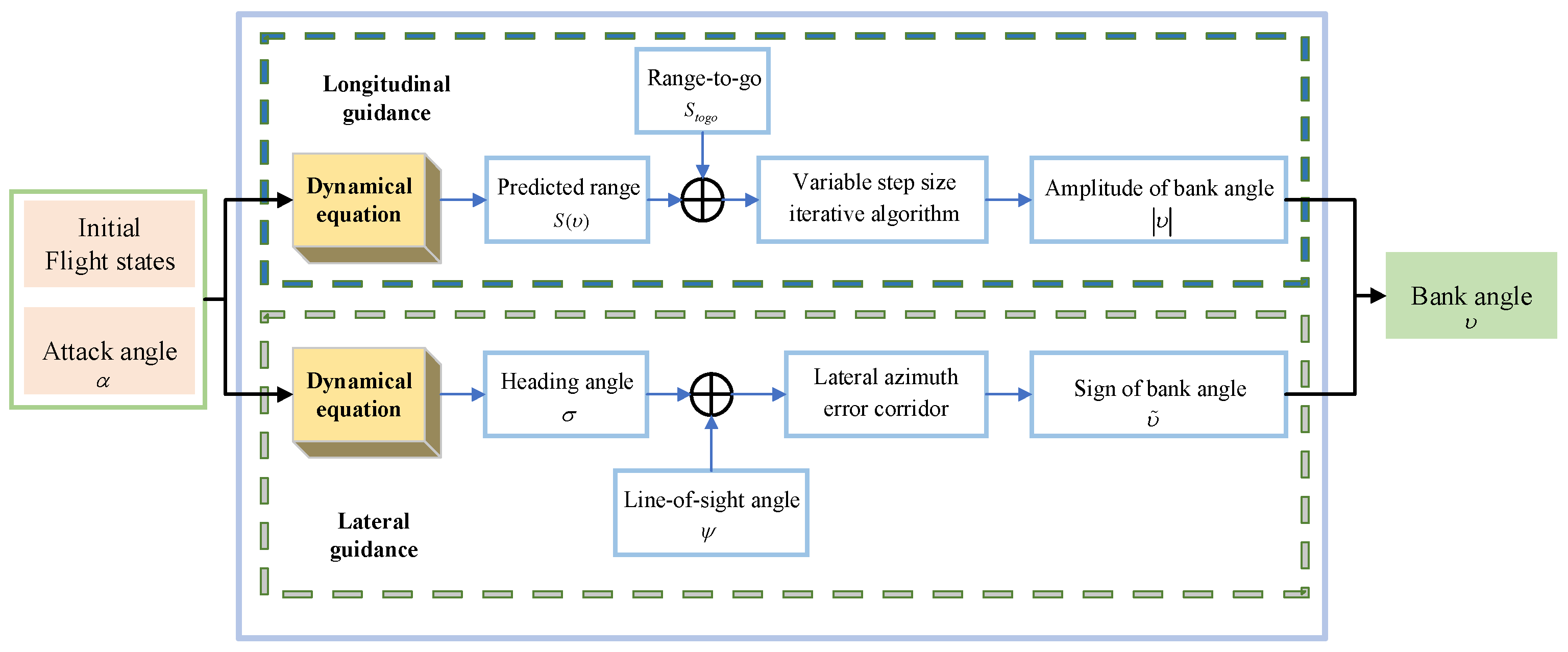
3. Predictor-Corrector Guidance Method

The superiority of predictor-corrector guidance is reflected in the accurate prediction of the flight trajectory, and the control variables of the predictor-corrector approach include attack angles and bank angles.

3.1. Design of Attack Angle

The attack angle is another key control quantity besides the bank angle, and it is determined by a preset curve that needs to consider the influence of different factors in the gliding flight. The thermal protection constraints of the vehicle are primarily considered in initial period, and the burden of thermal protection structure system can be effectively mitigated by setting a large attack angle. The lateral maneuvering capability and longitudinal voyage of vehicles can be significantly enhanced by setting the attack angle with the maximum lift-to-drag ratio. With comprehensive consideration, the attack angle curve is described as follows:

$$\alpha =\left\{\begin{array}{l}{\alpha }_{\max \hspace{1em}\hspace{1em}\hspace{1em}\hspace{1em}\hspace{1em}\hspace{1em}\hspace{1em}\hspace{1em}\hspace{1em}\hspace{1em}\hspace{1em}\hspace{1em}\hspace{1em}\hspace{1em}\hspace{1em}\hspace{1em}\hspace{1em}\hspace{1em}}{V}_A\le V_E\le V_0\hfill \\ \frac{{\alpha }_{\max L/D}-{\alpha }_{\max }}{V_2-V_1}(V_E-V_1)+{\alpha }_{\max \hspace{1em}\hspace{1em}\hspace{1em}}{V}_B\le V_E<V_A\hfill \\ {\alpha }_{\max L/D\hspace{1em}\hspace{1em}\hspace{1em}\hspace{1em}\hspace{1em}\hspace{1em}\hspace{1em}\hspace{1em}\hspace{1em}\hspace{1em}\hspace{1em}\hspace{1em}\hspace{1em}\hspace{1em}\hspace{1em}\hspace{1em}}{V}_{end}\le V_E<V_B\hfill \end{array}\right.$$

(7)

where ${\alpha }_{\max }$ means the maximum attack angle, and ${\alpha }_{\max L/D}$ is the attack angle that has the maximum lift-to-drag ratio. The notation $V_E$ represents the current velocity of the vehicle. The notations $V_0$ and $V_{end}$ denote the initial and terminal velocities of the vehicle. The notations $V_A$ and $V_B$ are the adjustable speed parameters.

3.2. Design of Bank Angle

The bank angle predictor based on the predictor-corrector method is illustrated in Figure 2.

3.2.1. Amplitude Design of Bank Angle

The amplitude of the bank angle $\left|\upsilon \right|$ is the key control quantity that determines whether the flight trajectory satisfies the terminal range and terminal velocity constraints. The bank angle amplitude is determined by the longitudinal trajectory design method based on the predictor-corrector method in this section.

The flight process constraints for reentry guidance can be converted into height–velocity constraints:

$$\left\{\begin{array}{l}H\ge hs\ln (\frac{{\rho }_0{k}^2{V}^{6.3}}{{\dot{Q}}^2{}_{\max }})\\ H\ge hs\ln (\frac{{\rho }_0{S}_m{V}^2\sqrt{C_L^2+C_D^2}}{2m{g}_0{n}_{\max }})\\ H\ge hs\ln (\frac{{\rho }_0{V}^2}{2q_{\max }})\end{array}\right.$$

(8)

Further, the height–velocity constraints can be converted into bank angle amplitude constraints:

$$\left\{\begin{array}{l}\left|{\upsilon }_{\dot{Q}}(V)\right|\le \arccos [(g-\frac{V^2}{r})\frac{2m{V}^{4.3}}{C_L{S}_m}(\frac{k}{{\dot{Q}}_{\max }}){ }^2]=\left|{\upsilon }_{{\dot{Q}}_{\max }}\right|\\ \left|{\upsilon }_n(V)\right|\le \arccos [(g-\frac{V^2}{r})\frac{\sqrt{1+{(\raisebox{1ex}{$C_D$}\!\left/ \!\raisebox{-1ex}{$C_L$}\right.)}^2}}{g_0{n}_{\max }}]=\left|{\upsilon }_{n_{\max }}\right|\\ \left|{\upsilon }_q(V)\right|\le \arccos [(g-\frac{V^2}{r})\frac{m}{C_L{q}_{\max }{S}_m}]=\left|{\upsilon }_{q_{\max }}\right|\end{array}\right.$$

(9)

where the notations $\left|{\upsilon }_{{\dot{Q}}_{\max }}\right|$, $\left|{\upsilon }_{n_{\max }}\right|$, and $\left|{\upsilon }_{q_{\max }}\right|$ represent the upper bounds of bank angle amplitude under the flight process constraints.

The height–velocity curve satisfying QEGC is solved by the variable step-size iterative algorithm (Algorithm 1).

Algorithm 1 Variable step-size iterative

1:  Initialization 2:  Set $\Delta H_{bound}>0$, $,\Delta h>0$$,i_{\max }$$,i=0$$,H=70 \mathrm{km}$ 3:   While $(i<i_{\max }$), do 4:   bring $H$ into formula (5) and get $\Delta H$ 5:   if $\left|\Delta H\right|\le \Delta H_{bound}$, do 6:    $H=H(i)$ 7:     end while 8:   elseif $\Delta H>\Delta H_{bound}$, do 9:    $H=H(i)+\Delta h$ 10:   elseif $\Delta H<-\Delta H_{bound}$, do 11:   $\Delta h=\Delta h/2$ 12:   $H=H(i)-\Delta h$ 13:  end 14:  Get H

When the upper bounds of the bank angle amplitude constraint are determined, the formula (1) is integrated in the longitudinal guidance period to obtain the predicted range $S(\upsilon )$ that satisfies the terminal energy constraint. The range-to-go is defined as follows:

$$S_{togo}=R_0\cdot \arccos [\sin \phi \sin {\phi }_{end}+\cos \phi \cos {\phi }_{end}\cos ({\lambda }_f-\lambda )]$$

(10)

The bank angle amplitude satisfying the requirements is obtained by solving the equation $S(\upsilon )-S_{togo}=0$ with the variable step-size iterative algorithm.

3.2.2. Sign Design of Bank Angle

The sign of the bank angle $\tilde{\upsilon }$ is the key heading control quantity that determines whether the flight trajectory can satisfy the terminal position constraints, and it is determined by the lateral trajectory design method based on the lateral azimuth error corridor.

Define the line-of-sight angle as

$$\psi =\arctan (\frac{\sin ({\phi }_{end}-\phi )}{\cos \lambda \tan {\lambda }_{end}-\sin \lambda \cos ({\phi }_{end}-\phi )})$$

(11)

The angular error of line-of-sight is formulated as the deviation between the heading angle and line-of-sight angle.

$$\Delta \psi =\sigma -\psi$$

(12)

The limiting range of the angular error of line-of-sight should be set in the lateral azimuth error corridor. It is regarded as too large a deviation from the terminal when the error is out of range, and the bank angle sign needs to be reversed to correct the trajectory. The error corridor is shown below:

$$\begin{array}{l}\Delta {\psi }_{up}=\left\{\begin{array}{l}\Delta {\psi }_{\max }\hspace{1em}\hspace{1em}\hspace{1em}\hspace{1em}\hspace{1em}\hspace{1em}\hspace{1em}\hspace{1em}\hspace{1em}\hspace{1em}\hspace{1em}\hspace{1em}\hspace{1em} V_{\Delta \psi }\le V\le V_0\\ \Delta {\psi }_{\max }-\frac{V_{\Delta \psi }-V}{V_{\Delta \psi }-V_{end}}(\Delta {\psi }_{\max }-\Delta {\psi }_{\min })\hspace{1em}\hspace{1em}\hspace{1em}{V}_{end}\le V\le V_{\Delta \psi }\end{array}\right.\\ \Delta {\psi }_{down}=-\Delta {\psi }_{up}\end{array}$$

(13)

where the notations $\Delta {\psi }_{up}$ and $\Delta {\psi }_{down}$ denote the top and bottom boundaries of the error corridor. The notations $\Delta {\psi }_{\max }$ and $\Delta {\psi }_{\min }$ represent the constant parameters, and $V_{\Delta \psi }$ is the turning speed when the error corridor becomes narrower.

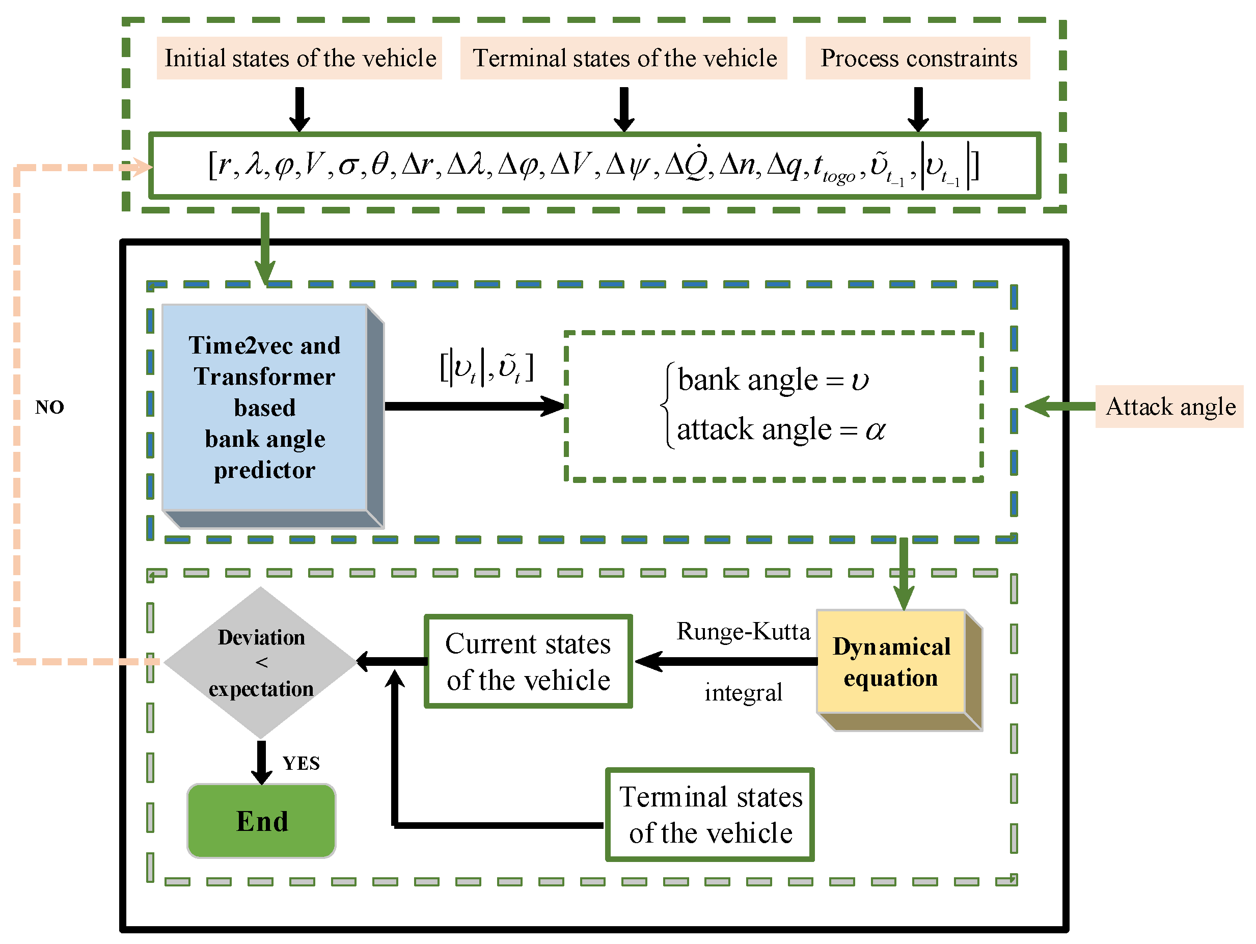
4. Predictive Reentry Guidance Based on Time2vec and Transformer Network

4.1. Inputs and Outputs of Network

The design of the reentry guidance law depends on the real-time vector of the vehicle states. In order to control the guidance accuracy and enhance the real-time performance, the state variables and state deviations of the vehicle are used as the initial network inputs, and the initial output is the bank angle. The following shortcomings are verified by model pre-training:

• The terminal speed out of bounds;
• The process constraints out of bounds;
• The prediction lag of the bank angle inversion.

Considering the above three drawbacks and the characteristics of the predictor-corrector algorithm, the inputs and outputs of the bank angle predictor are developed as follows:

$$\left\{\begin{array}{l}Inputs=[r,\lambda ,\phi ,V,\sigma ,\theta ,\Delta r,\Delta \lambda ,\Delta \phi ,\Delta V,\Delta \psi ,\Delta \dot{Q},\Delta n,\Delta q,t_{togo},{\tilde{\upsilon }}_{t_{-1}},\left|{\upsilon }_{t_{-1}}\right|]\\ Outputs=[\left|{\upsilon }_t\right|,{\tilde{\upsilon }}_t]\end{array}\right.$$

(14)

where the vector $[r,\lambda ,\phi ,V,\sigma ,\theta ,\Delta r,\Delta \lambda ,\Delta \phi ,\Delta V]$ contains the vehicle states and state deviations. The notation $\Delta \psi$ denotes the angular error of line-of-sight, which is used to restrict the reversal of bank angle. The vector $[\Delta \dot{Q},\Delta n,\Delta q]$ contains the deviations between process constraints and their peaks, which aims to limit the deviations of process constraints. The notation $t_{togo}$ denote the residual flight time of the vehicle, which is designed to limit the speed and flight capability of vehicle. The vector $[{\tilde{\upsilon }}_{t_{-1}},\left|{\upsilon }_{t_{-1}}\right|]$ contains the sign and amplitude of the bank angle at the last moment. The notations $\left|{\upsilon }_t\right|$ and ${\tilde{\upsilon }}_t\in \left\{1,-1\right\}$ denote the sign and amplitude of bank angle at the moment. Using the bank angle sign as a separate label increases the sensitivity of the predictor to the bank angle reversals.

The residual flight time of the vehicle is formulated as follows:

$$t_{togo}=\frac{S_{togo}}{V\cdot \cos \Delta \psi }$$

(15)

4.2. Bank Angle Predictor

The reentry guidance is a sequential decision-making process, and the data generated in the guidance process are continuous in time and have inherent sequential characteristics. Secondly, considering the credibility and stability of the model, it is necessary to notice the influence of historical data and avoid using the end-to-end sequence alignment algorithm when introducing deep learning into reentry guidance.

Vaswani et al. [22] proposes a new simple network architecture that eliminates recursion and convolution and calculates the conduction model between input and output completely based on the self-attention mechanism. Self-attention connects the different positions of a single sequence to calculate the representation of a sequence. It performs well on data with temporal characteristics and has been widely used in reading comprehension [23], temporal prediction [24], abstract summarization [25], and other tasks.

The transformer network can reduce the computational burden of processing high-dimensional input data. The data dimension is reduced by structurally selecting the subset of input, and the task processing system is more focused on finding the useful information related to the current output in the input data, to improve the quality of output. The transformer network in this paper is built based on the multi-head attention, and the multi-head attention is formulated as:

$$\left\{\begin{array}{l}MultiHead(Q,K,V)=Concat(hea{d}_1,\dots ,hea{d}_h)W^O\\ hea{d}_i=Attention(Q{W}_i^Q,K{W}_i^K,V{W}_i^V)\\ Attention(Q{W}_i^Q,K{W}_i^K,V{W}_i^V)=softmax(\frac{(Q{W}_i^Q){(K{W}_i^K)}^T}{\sqrt{d_k}})(V{W}_i^V)\end{array}\right.$$

(16)

where the projections are parameter matrices $W_i^Q\in {ℝ}^{d_{\mathrm{mod}el}\times d_k}$, $W_i^K\in {ℝ}^{d_{\mathrm{mod}el}\times d_k}$, and $W_i^V\in {ℝ}^{d_{\mathrm{mod}el}\times d_v}$. In this paper, we employ $h=12$ parallel attention layers, and for each of these we use $d_k=d_v=d_{\mathrm{mod}el}/h=256$. We compute the attention function on a set of queries simultaneously, packed together into a matrix $Q$. The keys and values are also packed together into matrices $K$ and $V$.

Time is an important feature in reentry guidance, and it is necessary to consider the temporal characteristics in the design of the bank angle predictor. Kazemi et al. [26] take an orthogonal but complementary approach by providing a model-agnostic vector representation for time, called Time2vec. We introduce the Time2vec to this work to improve the performance of the final predictor. For a given scalar notion of time $\tau$, its Time2vec is defined as follows:

$$\mathbf{t}\mathbf{2}\mathbf{v}(\tau )[i]=\left\{\begin{array}{l}{\omega }_i\tau +{\phi }_i\hspace{1em}\hspace{1em}\hspace{1em},\hspace{1em}\hspace{1em}if i=0.\\ \mathcal{F}({\omega }_i\tau +{\phi }_i)\hspace{1em}\hspace{1em},\hspace{1em}\hspace{1em}if 1\le i\le k.\end{array}\right.$$

(17)

where $\mathbf{t}\mathbf{2}\mathbf{v}(\tau )$ is a vector of size $k+1$, and $\mathbf{t}\mathbf{2}\mathbf{v}(\tau )[i]$ is the $i^{th}$ element of $\mathbf{t}\mathbf{2}\mathbf{v}(\tau )$. The notions ${\omega }_i$ and ${\phi }_i$ denote two learnable parameters. The notion $\mathcal{F}$ is a sine periodic activation function.

The bank angle predictor model built in this paper is shown in Figure 3, and the related parameter settings are expressed in

Table 1. Predictor model parameter settings.

Parameters	Value
batch size	128
timestep	100
feature number	17
output number	2
attention heads number	12
learning rate	0.0001
dropout rate	0.1

.

The prediction accuracy and speed are the primary considerations for setting network parameters and training parameters, and these two indicators are often contradictory. We determine the approximate range of parameters through some prior knowledge firstly and then use pre-training to determine the combination of parameters that performs well within the range.

The whole process of the Time2vec and transformer-based real-time trajectory optimization is shown in Figure 4:

5. Simulations and Analysis

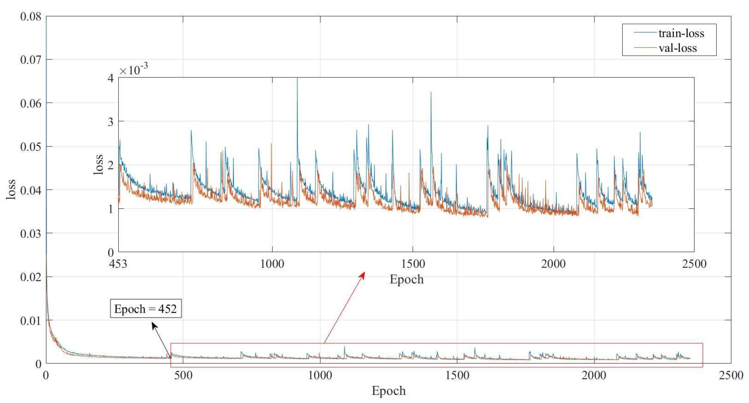
5.1. Bank Angle Predictor Training

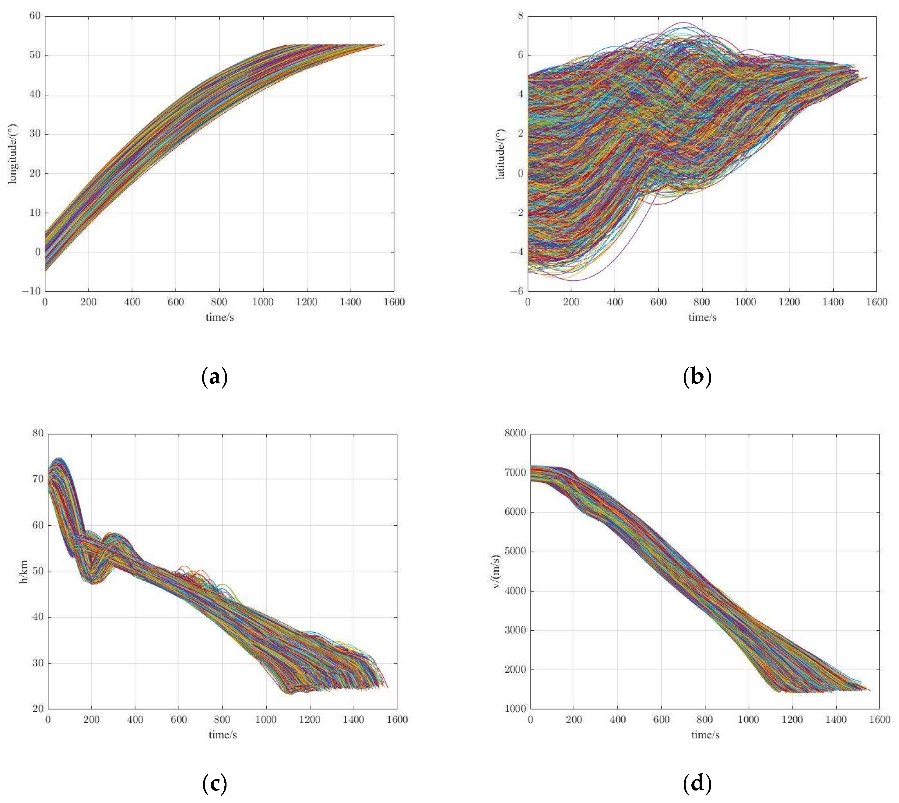
5.1.1. Generation of Training Datasets

The performance of the neural network model is closely related to the construction of data sets. At present, intelligent network algorithms for vehicle guidance can achieve reliable performance in the range of data sets. In order to improve the generalization of the predictor, the dataset constructed in this paper not only delineates the boundary at the initial point of the vehicle but also adds a Gaussian distribution error band coefficient to the drag coefficient, lift coefficient, aircraft mass, and atmospheric density during the guidance process, respectively. The

Table 2. The distributions of the aircraft parameters.

Parameters	Distributions
${\lambda }_0/(°)$	$U(-5,5)$
${\phi }_0/(°)$	$U(-5,5)$
$V_0/(\mathrm{m}/\mathrm{s})$	$U(6800,7200)$
${\theta }_0/(°)$	$U(85,95)$
$h_0/(\mathrm{km})$	$U(68,72)$
$\Delta C_D$	$N(0,{(5\%)}^2)$
$\Delta C_L$	$N(0,{(3\%)}^2)$
$\Delta m$	$N(0,{(1\%)}^2)$
$\Delta \rho$	$N(0,{(3\%)}^2)$

exhibits the parameter distributions.

Where the notations ${\lambda }_0$, ${\phi }_0$, $V_0$, ${\theta }_0$, and $h_0$ denote the initial states of the vehicle. The notations $\Delta C_D$, $\Delta C_L$, $\Delta m$, and $\Delta \rho$ represent the deviation coefficients of drag coefficient, lift coefficient, vehicle mass, and atmospheric density, respectively.

Other parameter settings mentioned above are display in

Table 3. Other parameter settings.

Parameters	Settings
${\rho }_0/(\mathrm{g}/\mathrm{L})$	1.225
$H_B/\mathrm{m}$	7200
$R_0/\mathrm{km}$	6378
$k$	5.188 × 10−8
${\dot{Q}}_{\max }/(\mathrm{KW}/{\mathrm{m}}^2)$	2000
$n_{\max }/\mathrm{g}$	10
$q_{\max }/\mathrm{kPa}$	500
${\alpha }_{\max }/(°)$	25
${\alpha }_{\max L/D}/(°)$	10
$V_A/(\mathrm{m}/\mathrm{s})$	3000
$V_B/(\mathrm{m}/\mathrm{s})$	5000

.

After setting all the parameters, 8000 trajectory data are generated randomly, and each trajectory is about 1370 sample points. The partition ratio of the training set, validation set, and test set is 8:1:1.

5.1.2. Predictor Training

Due to the large amount of ballistic data, considering the limitation of computing power, we adopt the method of incremental training to train the predictor. For each time, 200 ballistic data are input into the predictor model, and the total number of training epochs is 2350. We set a loss monitor in the training, and the monitor will collect loss values on the verification set in units of 50 epochs; then, the training will be terminated if the loss value of the 50th epoch does not decline compared to the 1st epoch. In order to get a suitable monitor threshold, we set a larger tolerance firstly, then reduce it gradually and observe the decreasing trend of loss values and the prediction accuracy. Finally, an excellent threshold is determined. Figure 5 displays the loss-epoch curve.

As we can see from Figure 5, with the increase of training generation, the loss function shows a decreasing trend and tends to converge on the training set and verification set. The first round of incremental training ended at $Epoch=452$, and the loss function showed a monotonic decreasing trend during the period. When $Epoch>452$, the loss curve is periodically oscillating and decreasing, which is caused by importing the pre-trained model during each round of incremental training.

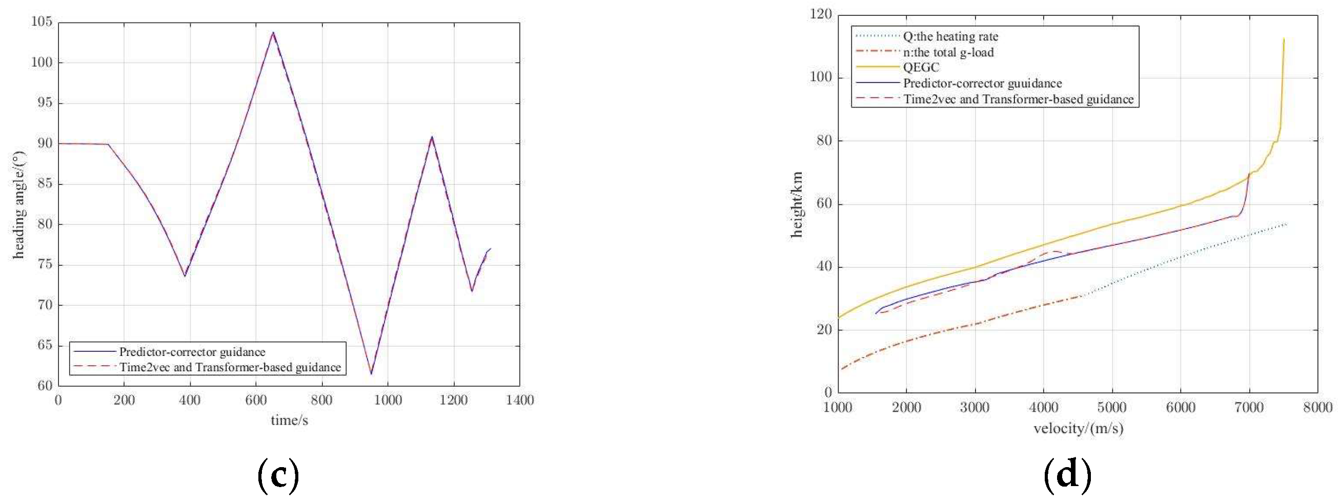
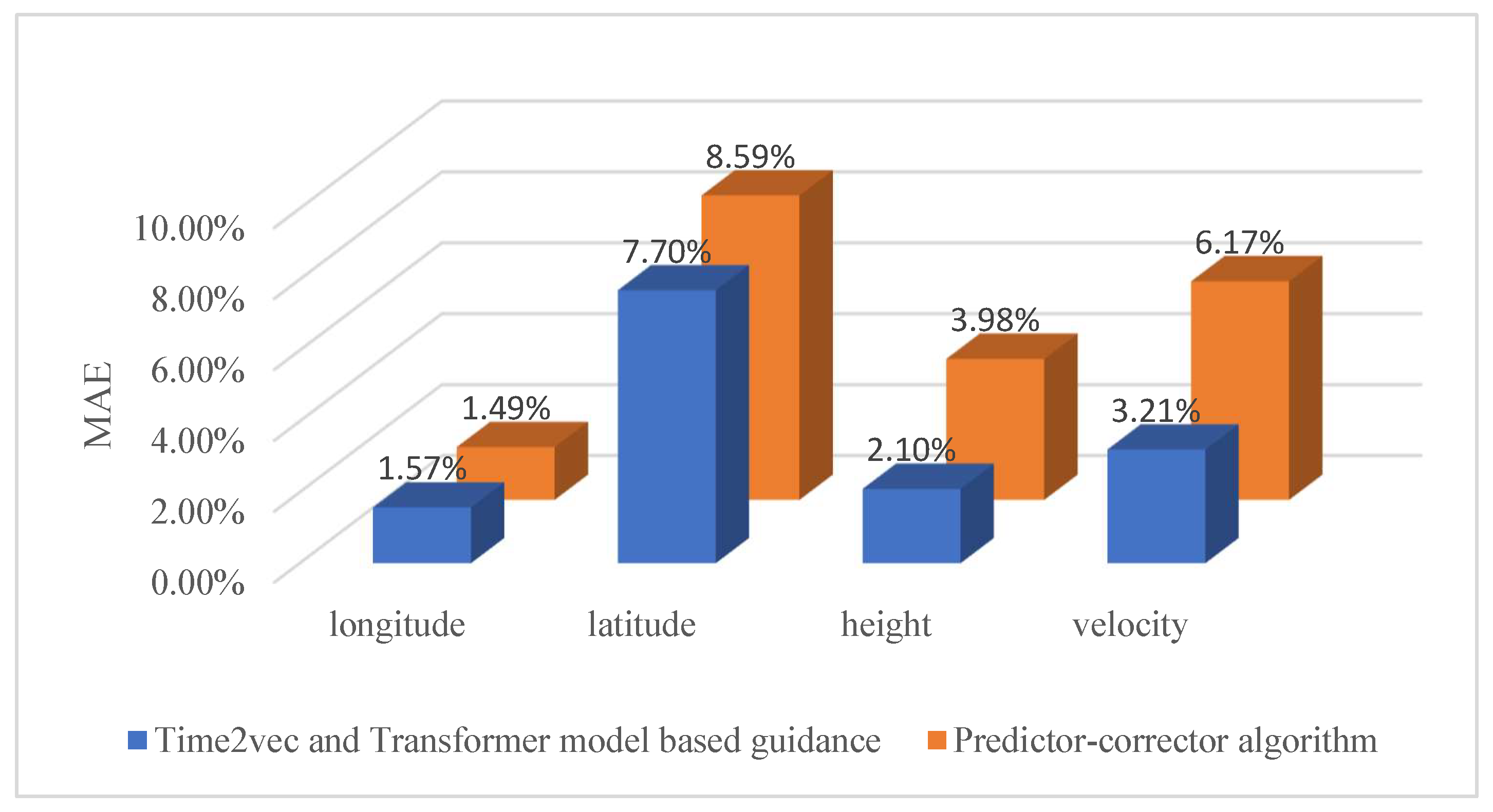
5.2. Evaluations on Guidance Precision

In this section, the guidance accuracy in the nominal environment is compared and analyzed based on one trajectory. Figure 6 displays the simulation results.

As can be seen from the Figures, the intelligent guidance based on the network can perfectly preserve the guidance precision of the predictor-corrector guidance. Figure 6d shows that the intelligent guidance satisfies the reentry flight corridor composed of three process constraints and QEGC. Therefore, the guidance law based on Time2vec and the transformer network is capable of completing the flight mission safely and reliably.

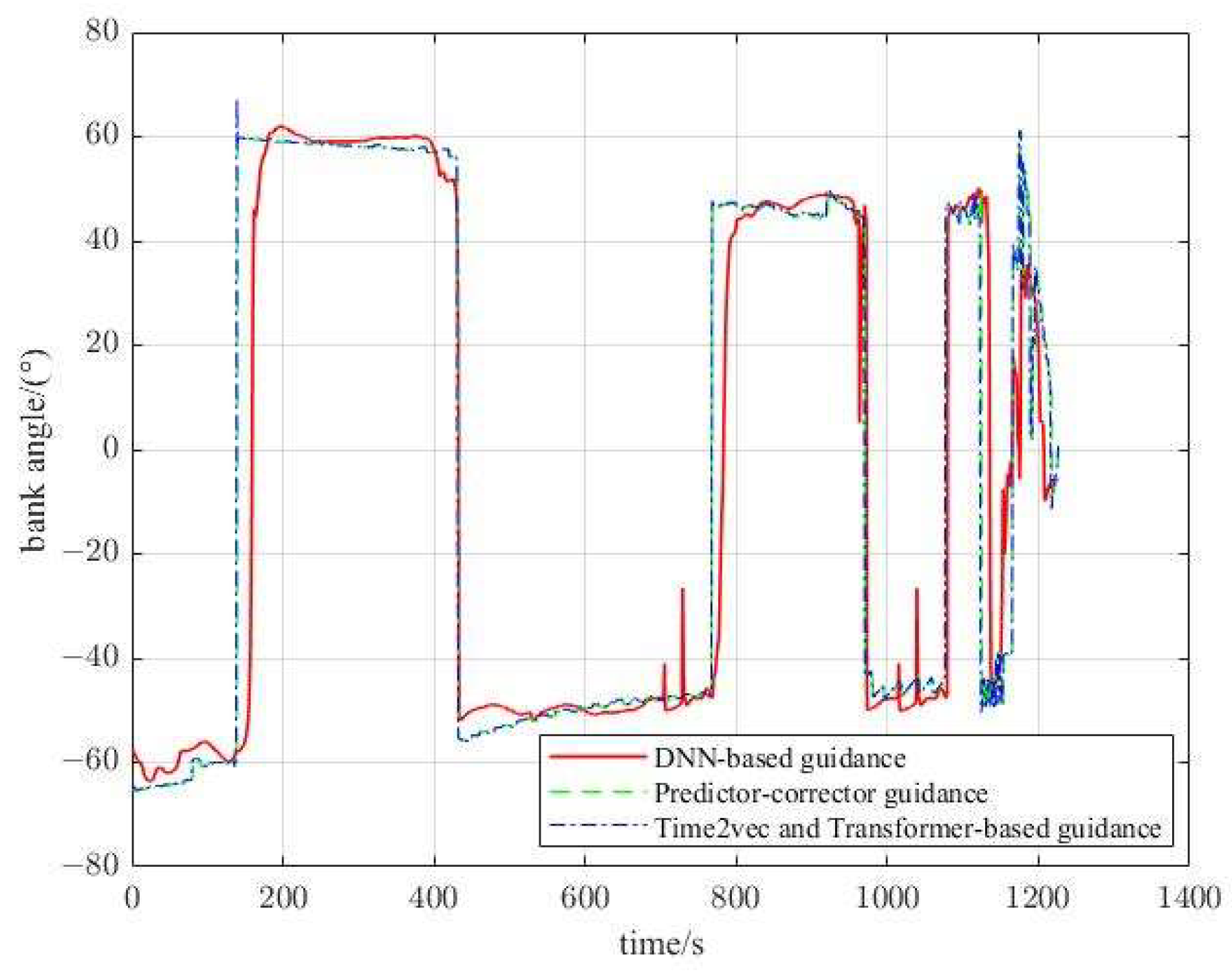
5.3. Evaluations on Bank Angle Prediction

Figure 7 displays the comparison of bank angle prediction between the temporal and non-temporal neural networks.

As can be seen from Figure 7, the transformer model has higher prediction accuracy and better adaptability to the reentry guidance.

5.4. Evaluations on Monte Carlo Simulations

In this section, the initial states and aerodynamic parameters follow the distributions listed in Table 2, and the variations are regenerated randomly. Under the condition of initial state errors and aerodynamic parameter perturbations, the trained transformer model is used to conduct 2000 groups of Monte Carlo simulations, and the results are shown in Figure 8.

To evaluate the accuracy and real-time performance of the guidance law based on the Time2vec and transformer model, we conduct 2000 groups of Monte Carlo simulations under the same conditions using the predictor-corrector guidance law. Figure 9 exhibits the mean absolute errors (MAE) of four terminal constraints, and Figure 10 shows the comparison of real-time performance.

According to Figure 9, the mean absolute errors of terminal longitude and latitude of the two guidance methods are relatively close. The reentry guidance law based on Time2vec and transformer has stricter restrictions on terminal height and speed. Compared with the traditional predictor-corrector guidance, the mean absolute error of terminal height is reduced by 47.29%, and the average absolute error of terminal speed decreased by 47.99%. Obviously, under initial state errors and aerodynamic parameter perturbations, the reentry guidance law based on Time2vec and the transformer is closer to the handover point and has stronger robustness to the deviation of parameters. There are three explanations for this. Firstly, various deviations and disturbances are considered in the generation of the training data set. Secondly, the training data are normalized before they are input into the predictor model, which reduces the sensitivity to the state deviations. Finally, the transformer model has natural generalization ability.

As we can see from Figure 10, the average time needed to complete a reentry flight based on the guidance model of Time2vec and the transformer is 10.99 s, in which the time of completing the bank angle prediction is 8.84 s, the time of data preprocessing is 0.05 s, and the time of the other operations is 2.1 s. The average flight time of the predictor-corrector guidance to complete a reentry phase is 53.76 s, in which the longitudinal guidance process takes 51.65 s, the lateral guidance takes 0.01 s, and other operations take 2.1 s. Compared with the traditional predictor-corrector guidance, the average time required to complete the same reentry flight is reduced by 79.56%, and the real-time performance of the guidance is significantly improved.

6. Conclusions

In this article, a real-time reentry guidance method for hypersonic vehicles is presented in detail. The proposed strategy formalizes the guidance period and makes the guidance law rapid, high-precision, robust, reliable, and adaptive. We present the guidance architecture and design process and test the method on the reentry guidance in simulation. Comparative studies are carried out between the Time2vec and transformer-based guidance and the predictor-corrector guidance to illustrate the improved performance. The Time2vec and transformer-based guidance can provide a feasible guidance policy to accelerate the bank angle prediction process and has the capabilities of adaptation and robustness against the initial state errors and aerodynamic parameter perturbations, by involving the neural network.

References

1. Lu, P. Entry guidance: A unified method. J. Guid. Control. Dyn. 2014, 37, 713–728. [Google Scholar] [CrossRef]
2. Guo, Y.; Li, X.; Zhang, H.; Wang, L.; Cai, M. Entry guidance with terminal time control based on quasi-equilibrium glide condition. IEEE Trans. Aerosp. Electron. Syst. 2019, 56, 887–896. [Google Scholar] [CrossRef]
3. Xue, S.; Lu, P. Constrained predictor-corrector entry guidance. J. Guid. Control. Dyn. 2010, 33, 1273–1281. [Google Scholar] [CrossRef]
4. Wang, T.; Zhang, H.; Zeng, L.; Tang, G. A robust predictor–corrector entry guidance. Aerosp. Sci. Technol. 2017, 66, 103–111. [Google Scholar] [CrossRef]
5. Cheng, L.; Jiang, F.; Wang, Z.; Li, J. Multiconstrained real-time entry guidance using deep neural networks. IEEE Trans. Aerosp. Electron. Syst. 2020, 57, 325–340. [Google Scholar] [CrossRef]
6. Zhang, D.; Liu, L.; Wang, Y. On-line reentry guidance algorithm with both path and no-fly zone constraints. Acta Astronaut. 2015, 117, 243–253. [Google Scholar] [CrossRef]
7. Wang, X.; Guo, J.; Tang, S.; Qi, S.; Wang, Z. Entry trajectory planning with terminal full states constraints and multiple geographic constraints. Aerosp. Sci. Technol. 2019, 84, 620–631. [Google Scholar] [CrossRef]
8. Xu, J.; Qiao, J.; Guo, L.; Chen, W. Enhanced predictor–corrector Mars entry guidance approach with atmospheric uncertainties. IET Control. Theory Appl. 2019, 13, 1612–1618. [Google Scholar]
9. Lu, P.; Forbes, S.; Baldwin, M. Gliding Guidance of High L/D Hypersonic Vehicles. In Proceedings of the AIAA Guidance, Navigation, and Control (GNC) Conference, Boston, MA, USA, 19–22 August 2013; Available online: https://arc.aiaa.org/doi/10.2514/6.2013-4648 (accessed on 6 July 2022).
10. Sivan, K.; Savithri, A.S.; Ashok, J. An Adaptive Reentry Guidance; Indian Institute of Technology Bornbay: Mumbai, India, 2004. [Google Scholar]
11. Li, Z.; Sun, X.; Hu, C.; Liu, G.; He, B. Neural network based online predictive guidance for high lifting vehicles. Aerosp. Sci. Technol. 2018, 82–83, 149–160. [Google Scholar] [CrossRef]
12. Alzubaidi, L.; Zhang, J.; Humaidi, A.J.; Al-Dujaili, A.; Duan, Y.; Al-Shamma, O.; Santamaría, O.; Fadhel, M.A.; Al-Amidie, M.; Farhan, L. Review of deep learning: Concepts, CNN architectures, challenges, applications, future directions. J. Big Data 2021, 8, 1–74. [Google Scholar] [CrossRef] [PubMed]
13. Liu, J.; Wang, M.; Li, S. The rapid data-driven prediction method of coupled fluid-thermal-structure for hypersonic vehicles. Aerospace 2021, 8, 265. [Google Scholar] [CrossRef]
14. Strijhak, S.; Ryazanov, D.; Koshelev, K.; Ivanov, A. neural network prediction for ice shapes on airfoils using icefoam simulations. Aerospace 2022, 9, 96. [Google Scholar] [CrossRef]
15. Wang, N.; Er, M.J. Self-constructing adaptive robust fuzzy neural tracking control of surface vehicles with uncertainties and unknown disturbances. IEEE Trans. Control. Syst. Technol. 2014, 23, 991–1002. [Google Scholar]
16. Hu, R.; Zhang, Y. Fast path planning for long-range planetary roving based on a hierarchical framework and deep reinforcement learning. Aerospace 2022, 9, 101. [Google Scholar] [CrossRef]
17. Du, X.; Chen, J.; Zhang, H.; Wang, J. Fault detection of aero-engine sensor based on inception-CNN. Aerospace 2022, 9, 236. [Google Scholar] [CrossRef]
18. Wang, J.; Wu, Y.; Liu, M.; Yang, M.; Liang, H. A real-time trajectory optimization method for hypersonic vehicles based on a deep neural network. Aerospace 2022, 9, 188. [Google Scholar] [CrossRef]
19. Horn, J.F.; Schmidt, E.M.; Geiger, B.R.; DeAngelo, M.P. Neural network-based trajectory optimization for un-manned aerial vehicles. J. Guid. Control. Dyn. 2012, 35, 548–562. [Google Scholar] [CrossRef]
20. Shi, Y.; Wang, Z. A Deep Learning-Based Approach to Real-Time Trajectory Optimization for Hypersonic Vehicles. In Proceedings of the AIAA Guidance, Navigation, and Control (GNC) Conference, Orlando, FL, USA, 6–10 January 2020; Available online: https://arc.aiaa.org/doi/10.2514/6.2020-0023 (accessed on 6 July 2022).
21. Xu, M.; Chen, K.; Liu, L.; Tang, G. Quasi-equilibrium glide adaptive guidance for hypersonic vehicles. Sci. China Technol. Sci. 2012, 55, 856–866. [Google Scholar] [CrossRef]
22. Vaswani, A.; Shazeer, N.; Parmar, N.; Uszkoreit, J.; Jones, L.; Gomez, A.N.; Kaiser, Ł.; Polosukhin, I. Attention is All You Need; Curran Associates Inc.: Red Hook, NY, USA, 2017; Volume 30, pp. 6000–6010. [Google Scholar]
23. Cheng, J.; Dong, L.; Lapata, M. Long Short-Term Memory-Networks for Machine Reading. 2016. Available online: https://arxiv.org/abs/1601.06733 (accessed on 6 July 2022).
24. Malibari, N.; Katib, I.; Mehmood, R. Predicting stock closing prices in emerging markets with transformer neural networks: The saudi stock exchange case. Int. J. Adv. Comput. Sci. Appl. 2021, 12, 878–886. [Google Scholar] [CrossRef]
25. Paulus, R.; Xiong, C.; Socher, R. A Deep Reinforced Model for Abstractive Summarization. 2017. Available online: https://doi.org/10.48550/arXiv.1705.04304 (accessed on 6 July 2022).
26. Kazemi, S.M.; Goel, R.; Eghbali, S.; Ramanan, J.; Sahota, J.; Thakur, S.; Wu, S.; Smyth, C.; Poupart, P.; Brubaker, M. Time2vec: Learning a Vector Representation of Time. 2019. Available online: https://doi.org/10.48550/arXiv.1907.05321 (accessed on 6 July 2022).
Figure 1. A schematic diagram of the reentry guidance system.
Aerospace 09 00427 g001
Figure 2. The predictor of bank angle based on predictor-corrector method.
Aerospace 09 00427 g002
Figure 3. The Time2vec and transformer-based bank angle predictor models.
Aerospace 09 00427 g003
Figure 4. The time2vec and transformer-based real-time trajectory optimization.
Aerospace 09 00427 g004
Figure 5. The loss-epoch curve.
Aerospace 09 00427 g005
Figure 6. The comparison curves. (a) A comparison of the longitude–latitude curve; (b) comparison of flight-path angle curve; (c) comparison of heading angle curve; and (d) comparison of velocity–height curve.
Aerospace 09 00427 g006aAerospace 09 00427 g006b
Figure 7. A comparison of time-bank angle curve.
Aerospace 09 00427 g007
Figure 8. The simulations under initial state errors and aerodynamic parameter perturbations. (a) Time–longitude curve; (b) time–latitude curve; (c) time–height curve; and (d) time–velocity curve.
Aerospace 09 00427 g008
Figure 9. A comparison of terminal constraints-MAE.
Aerospace 09 00427 g009
Figure 10. A comparison of real-time performance.
Aerospace 09 00427 g010