Article

Short-Term Trajectory Prediction Based on Hyperparametric Optimisation and a Dual Attention Mechanism

College of Air Traffic Management, Civil Aviation Flight University of China, Guanghan 618307, China
*
Authors to whom correspondence should be addressed.
Aerospace 2022, 9(8), 464; https://doi.org/10.3390/aerospace9080464
Submission received: 16 June 2022 / Revised: 14 August 2022 / Accepted: 18 August 2022 / Published: 20 August 2022

Abstract

:
Highly accurate trajectory prediction models can achieve route optimisation and save airspace resources, which is a crucial technology and research focus for the new generation of intelligent air traffic control. Aiming at the problems of inadequate extraction of trajectory features and difficulty in overcoming the short-term memory of time series in existing trajectory prediction, a trajectory prediction model based on a convolutional neural network-bidirectional long short-term memory (CNN-BiLSTM) network combined with dual attention and genetic algorithm (GA) optimisation is proposed. First, to autonomously mine the data association between input features and trajectory features as well as highlight the influence of important features, an attention mechanism was added to a conventional CNN architecture to develop a feature attention module. An attention mechanism was introduced at the output of the BiLSTM network to form a temporal attention module to enhance the influence of important historical information, and GA was used to optimise the hyperparameters of the model to achieve the best performance. Finally, a multifaceted comparison with other typical time-series prediction models based on real flight data verifies that the prediction model based on hyperparameter optimisation and a dual attention mechanism has significant advantages in terms of prediction accuracy and applicability.

1. Introduction

Problems such as air traffic congestion, flight delays, and reduced transport efficiency considerably threaten air traffic safety. Making full use of valuable airspace resources, managing air flow efficiently, and solving problems such as airspace conflicts, large flight delays, and aviation safety are urgently required [1].
Countries such as European countries and the USA have researched four-dimensional (4D) trajectory to address these issues [2], and they have proposed a trajectory-based (TBO) operating concept. TBO is based on 4D trajectory throughout the entire flight cycle, with real-time exchange of trajectory dynamics between airports, crews, as well as air traffic control. There is a deep collaboration between all relevant parties to ensure that the entire flight cycle is “controlled and accessible”. The literature published by the International Civil Aviation Organisation (ICAO) [3,4] also adopts the TBO concept using an engineering approach to improve four aspects: efficient flight paths, airport operations, systems and data, as well as optimal capacity. Trajectory prediction is an important technique for TBO [5,6], as accurate trajectory prediction directly affects the performance of aircraft flight management, traffic management, anomalous behaviour detection, and many other aspects.
With the constant update of civil aviation equipment and technological development, the demand for accurate and real-time trajectory prediction has increased, and prediction methods are constantly being updated. The main categories are as follows:
  • Kinetic models: Kinetic-based trajectory prediction models focus on the relationship between the forces acting on an aircraft and their motion. Zhang et al. [7] reduced the uncertainty of trajectory prediction by analysing model construction, aircraft intent, performance parameters, and other factors. Based on BADA data, He et al. [8] established a model for the change in parameters such as dynamics, meteorology, and flight path to achieve accurate trajectory prediction. Kang et al. [9] established an aircraft mass estimation model and an altitude profile prediction model based on real-time trajectory data. Lee et al. [10] proposed a stochastic system tracking model and an estimated-time-of-arrival prediction algorithm to construct a nonlinear dynamic model under multiple flight modes. Dynamical models require many parameters owing to the consideration of information such as aircraft performance, some of which are commercially sensitive, and others are obtained using estimates from existing databases. The prediction accuracy of the model is significantly reduced when the data resources are limited.
  • State estimation model: The actual flight process can be considered a state transfer. Trajectory prediction estimates the state, such as latitude, longitude, and altitude, generated by the model during the flight. Chen et al. [11] constructed aircraft state equations based on known flight trajectory points, and they completed accurate trajectory prediction using an unscented Kalman filter. Lv et al. [12] improved the current Kalman filter (MIEKF) prediction system using multi-information theory to predict 4D trajectory in different states accurately. Zhou et al. [13] used the Kalman filter for track prediction, which is more suitable for single-step prediction than other models with significant short-term predictions. Tang et al. [14] used the IMM algorithm to track the aircraft’s trajectory using a geodetic coordinate system to represent the aircraft’s position and build each directional sub-model separately. The state estimation model is relatively simple, but it can lead to large errors owing to the inability to capture aircraft manoeuvre uncertainty accurately over long periods.
  • Machine learning-based model: Machine learning has achieved great success in speech recognition, style migration, and image classification. Therefore, machine learning has also been applied to time-series data processing. Examples include pedestrian and vessel trajectory and traffic flow predictions [15,16,17]. Trajectory clustering is a clustering analysis of historical trajectories [18,19] that combines updated state information to correct prediction results and improve the prediction accuracy. Yin et al. [20] constructed a four-dimensional trajectory prediction model by analysing wind data in GRIB format. Pang et al. [21] proposed a Convolutional LSTM (ConvLSTM) to extract important features from weather information to solve pre-takeoff and convective weather-related trajectory prediction problems. Chen et al. [22] proposed a trajectory prediction model based on the attention mechanism and generative adversarial network to address problems such as the inability of the LSTM network to extract key information effectively for trajectory prediction. Shi et al. [23] proposed an online updated LSTM short-term prediction algorithm to address the influence of different factors in the navigation process on the current trajectory. Wang et al. [24] designed a training model with different K values and obtained an optimal parametric model by comparing the accuracies of different K values. Currently, LSTM neural networks are primarily used for trajectory prediction [25,26,27,28]. Hybrid models of CNN-LSTM are also widely used for prediction tasks [29,30]; however, these models have problems such as insufficient extraction of important features.
To address the current problems arising in short-term trajectory prediction, we begin with a hybrid neural network based on an attention mechanism. The innovative points are as follows:
a.
By introducing the dual attention mechanism into the convolutional-bidirectional long short-term memory network (CNN-BiLSTM) model, the CNN was used to extract the trajectory space features, and the feature attention module achieved the mining of important features in the raw data and enhanced their impact by weighting the distribution of the CNN output. The subsequent BiLSTM module mines the trajectory temporal features, and the temporal attention module extracts important historical information based on the influence of each time node in the hidden layer state of the BiLSTM on the forecasting results, enhancing the learning of interdependencies in the time step. Thus, full integration of temporal features at the prediction points was achieved. The problem of important high-dimensional feature extraction and the long-term dependence of the time series was effectively solved. To the best of our knowledge, this is the first application of the DA-CNN-BiLSTM model to trajectory prediction.
b.
The use of genetic algorithms (GA) to optimise the hyperparameters of the entire model ensures the optimal learning capability of the model, overcoming the shortcomings of manual parameter tuning, which is experience-dependent, time-consuming, and has poor stability.
c.
The performances of the different models in trajectory prediction were systematically investigated. Three sets of comparisons were made. Specifically, the role of introducing CNN in extracting spatial features of the trajectory data was investigated. The bi-directional temporal feature extraction capability of the BiLSTM was verified by comparing BiLSTM to LSTM. In addition, a comparative analysis of temporal attention (T-CNN-BiLSTM), feature attention (F-CNN-BiLSTM), and dual attention (DA-CNN-BiLSTM) was conducted to investigate the impact of feature attention and temporal attention mechanisms on the prediction accuracy.
The remainder of this paper is organised as follows. Section 2 analyses the Automatic Dependent Surveillance-Broadcast (ADS-B) data and their preprocessing. Section 3 describes the modelling approach and framework structure of this study. The experimental simulations and comparative analysis are performed in Section 4. The final section concludes the study and suggests possible future research directions.

2. ADS-B Data Analysis and Processing

ADS-B is an aircraft operational surveillance technology [31] that automatically transmits 4D position data from airborne equipment as well as identification information to the ground equipment station via a ground–air–data link.

2.1. ADS-B Properties

ADS-B data contain many attributes, including flight number, reception time, flight altitude, latitude, longitude, ground speed, and heading. Among them, the trajectory characteristics consist of flight altitude, latitude, longitude, and time, whereas other attributes comprise the position information and flight status.
T = { T 1 , T 2 , , T r } ,
T r = { t 1 , u 1 , g 1 , t 2 , u 2 , g 2 , , t m , u m , g m } ,
u = ( u l o n , u l a t , u a l t ) ,
g = ( g n , g s , g d ) ,
where T indicates the historical trajectory of the flight for the past r days, and T r indicates the trajectory at m successive times. With t , u , g , the position information u and other flight status characteristics g received at time t are indicated, where u includes longitude ( u l o n ), latitude ( u l a t ), and altitude ( u a l t ), whereas g includes the flight number ( g n ), ground speed ( g s ), and heading ( g d ).

2.2. Preprocessing of the ADS-B Trajectory

Owing to the high frequency of ADS-B transmissions, the large number of duplicate data, and the uneven time intervals, the data were processed by first removing duplicate and null values, filtering the time intervals greater than or equal to 1 s, deleting data with intervals less than 1 s, and interpolating the data with three-spline interpolation for data greater than 2 s to facilitate learning and prediction. After redundant interpolation, the time intervals were averaged as Δt = 5 s.
If there is less information in the trajectory data, training may result in insufficient retention of key information and discarding of perturbation information owing to insufficient constraints or lack of information, resulting in an insufficient generalisation capability and prediction accuracy of the model. Therefore, the following features were fused into the dataset through the feature construction:
d is the distance of each trajectory point from reference point R . We chose the centre of the landing field as the reference point R ( x r e f , y r e f , z r e f ) , and distance d m i was calculated according to the following equation:
d m i = ( x m i x r e f ) 2 + ( y m i y r e f ) 2 + ( z m i z r e f ) 2
The angle θ between each trajectory point and the reference point R shows the state of change in the trajectory relative to the reference point (steering state). θ was calculated according to the following equation:
θ i m = a r c t a n ( y m i y r e f x m i x r e f )
To avoid discontinuities at ± p , the sine and cosine values of θ , sin θ i m , and cos θ i m were used instead of θ i m . In the follow-up process, the trajectory was considered as a time series and no timestamp information was required; therefore, the sequence of trajectories for the m trajectory point of the i trajectory was X i = { ( x m i , y m i , a m i , v m i , d m i , sin θ i m , sin θ i m ) R + m = 1 , 2 , , m } . The characteristics of the trajectory points are listed in Table 1.
Normalisation: The data must be normalised to eliminate the effects of different magnitudes.
N = X m i n max m i n
where X is the original sample, m a x is the maximum, m i n is the minimum, and N is the normalised sample.

2.3. Sample Construction

We divided the trajectory data into training samples and labels, and a sample of the trajectory sample construction is shown in Figure 1.
The time steps are represented by rows and features X are represented by columns in the figure, and we take a single-step prediction with a time step of 6. That is, the first six rows of features s a m p l e 1 = { l a t , l o n , a l t , v e l , h , d , s i n , c o s { } } are used to predict the next point, Y 1 = { l a t , l o n , a l t } .

3. Methods

3.1. CNN Network

Currently, the CNN [32] is a popular deep learning model. It uses convolutional operations to achieve a higher-dimensional representation of the original data, which can effectively extract internal features from the original data. The CNN structure is shown in Figure 2 and it consists of convolutional, pooling, and fully connected layers. The model formulation is shown in Equations (8)–(10).
C = f ( X w c + b c ) ,
P = δ ( C ) + b p ,
H = φ ( P × w s + b s ) ,
where C and P are the outputs of the convolutional and pooling layers, respectively; H is the feature vector of the CNN output; w c and w s are the weight matrices of the convolution and fully connected layers, respectively; b c , b p , and b s are the bias vectors of the convolution, pooling, and fully connected layers, respectively; is the convolutional operation; f ( ) is the activation function of the convolution layer; δ ( ) is the pooling method. This study adopts one-dimensional convolution and maximum pooling.

3.2. BiLSTM Network

The LSTM adds three logical gating units to the recurrent neural network (RNN): forget, input, and output gates. The LSTM can achieve stable learning at multiple time steps and effectively model the time-dependent manner [33]. The structure of the LSTM network is illustrated in Figure 3.
The input gate selects the current state to be retained, the forgetting gate selects the previous state to be forgotten, and the output gate selects the current state to be output to hidden state h t . The LSTM network is calculated according to Equations (11)–(15).
i t = Sigmoid ( w i x t + u i h t 1 + b i ) ,
f t = Sigmoid ( w f x t + u f h t 1 + b f ) ,
o t = Sigmoid ( w o x t + u o h t 1 + b o ) ,
S t = tanh ( w g x t + u g h t 1 + b g ) i t + S t 1 f t ,
h t = tanh ( S t ) o t ,
where i t , f t , o t , S t , and h t are the state matrices of the ingate, forget gate,output gate, memorial units, and output unit, respectively; w i , w f , w o , and w g are the weight matrices corresponding to the input at the current moment; u i , u f , u o , and u g are the weight matrices corresponding to the output at the previous moment; b i , b f , b o , and b g are the corresponding bias vectors; represents the multiplication of the elements of the matrix at the corresponding positions.
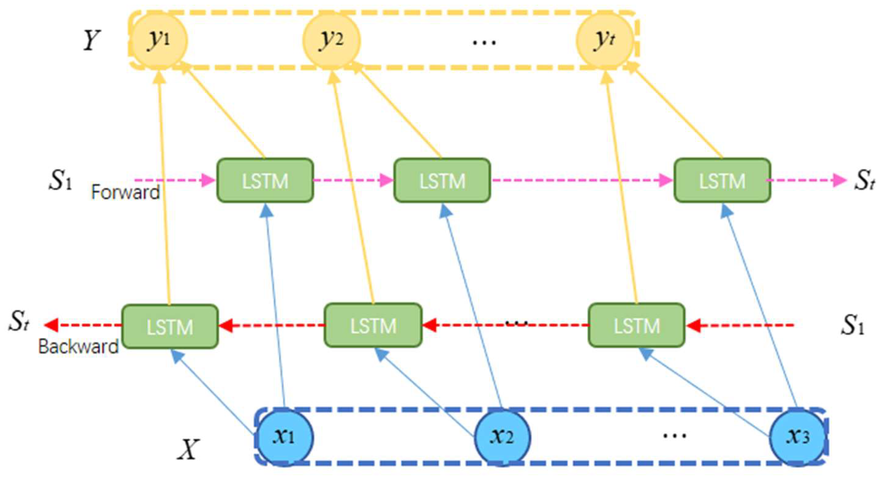
The BiLSTM [34] network is a two-layer LSTM network consisting of a combination of forward and reverse LSTM layers. The network structure of the BiLSTM is shown in Figure 4.

3.3. Attention Mechanism

The attention mechanism addresses the features of the target that we want to detect by assigning attention to the input weights, thereby implementing the attention mechanism [35]. Using the attention mechanism to achieve time-series model building can enhance the precision of the model [36,37]. The core idea is to assign different weights to the hidden layer states by reasonably allocating attention to different input information to highlight the influence of important information on the results. The weight assignment calculation of the attention mechanism can be expressed according to Equations (16)–(17).
e t = u a tanh ( w a h t + b a )  
a t = exp ( e t ) j = 1 t e j ,
where h t is the hidden layer state vector of the neural network at moment t ; e t is the attention probability distribution; a t is the attention score; w a is the weight vector; b a is the bias vector.

3.4. DA-CNN-BiLSTM Model

3.4.1. Feature Attention

The feature attention module is a combination of a CNN and an attention mechanism. The model focuses on important features by dynamically assigning attention weights to the input features and mining the association between the input and target features. The model is shown in Figure 5. At the t time step, a single-time input feature vector x t = [ x 1 , t ,   x 2 , t ,   ,   x M , t ] containing M features. A single-layer neural network is used to calculate the attention weight vector e t [38]:
e t = σ ( W e x t + b e ) ,
where e t = [ e 1 , t ,   e 2 , t ,   ,   e M , t ] is the combination of attention weight coefficients corresponding to each input feature at the current moment t ; W e is the trainable weight matrix; b e is the bias vector for calculating the feature attention weights; σ ( · ) is the Tanh activation function.
The Softmax function in Equation (19) normalises the attention weight coefficients [38] to obtain the attention weight of the feature α t = [ α 1 , t ,   α 2 , t ,   ,   α m , t ,   ,   α M , t ] , where α m , t is the attention weight value of the m feature.
α m , t = e x p ( e m , t ) i = 1 M e i , t ,
recalculates the input feature vector x t as a weighted vector h t * :
h t * = α t · x t = [ α 1 , t x 1 , t     α 2 , t x 2 , t         α M , t x M , t ] ,
where denotes the Hadamard product.

3.4.2. Temporal Attention

After the input data have been passed through the feature attention module, the key feature information is captured by BiLSTM two-way learning, which captures the temporal variation pattern within the sequence. The attention mechanism assigns different weights to the hidden states of the BiLSTM output according to the degree of association between the historical nodes and the results. The model is shown in Figure 6. The input is the state h t = [ h 1 , t ,   h 2 , t ,   ,   h k , t ] of the hidden layer of the BiLSTM network cell as the model is iterated to moment t , where k is the length of the time window of the input sequence. The vector of temporal attention weights l t for the current moment t corresponding to each historical moment [38] is:
l t = ReLU ( W d h t + b d ) ,
where l t = [ l 1 , t ,   l 2 , t ,   ,   l k , t ] ; W d is the trainable weight matrix; b d is the bias vector for calculating the temporal attention weights; RelU ( · ) denotes the activation function to increase the feature variance and make the weight assignment more focused.
The Softmax function normalises the attention weight coefficients at each time to obtain the temporal attention weight β t = [ β 1 , t ,   β 2 , t ,   ,   β τ , t ,   ,   β k , t ] , where β τ , t is the attention weight value at the t time, and then the hidden layer states at each corresponding historical moment are weighted to obtain the integrated temporal information state h s * .
β τ , t = exp ( l τ , t ) j = 1 k l j , t ,
h s * = h t β t = τ = 1 k β τ , t h τ , t ,
where denotes the matrix product.

3.4.3. DA-CNN-BiLSTM Trajectory Prediction Model

As typical multidimensional time-series data, flight trajectory data contain mapping relationships between historical time and future time trajectory points. To address the complex mapping relationships, we proposed a DA-CNN-BiLSTM trajectory prediction model, as shown in Figure 7, which is a combination of the CNN and an attention mechanism. The CNN can fully exploit high-dimensional features with convolution and pooling, and the attention mechanism trains the weights of the high-dimensional features to ensure that the key features play an important role. The temporal attention module is a combination of a BiLSTM network, which learns periodic and trending features from time-series data, and an attention mechanism. The attention mechanism is trained with hidden state weights to select important historical serial state information autonomously, overcoming the problem of information loss and gradient disappearance that BiLSTM networks are prone to when faced with longer serial inputs, and highlighting the impact of temporal state on prediction results.

4. Case Analysis

Here, the model parameters were identified using GA for hyperparameter search and validation using real data. Finally, three sets of models were set up for comparison to clarify the role of CNNs and Bi-LSTMs as well as the importance of attention models in short-term trajectory prediction. The model was based on TensorFlow 2.0.

4.1. Experimental Datasets

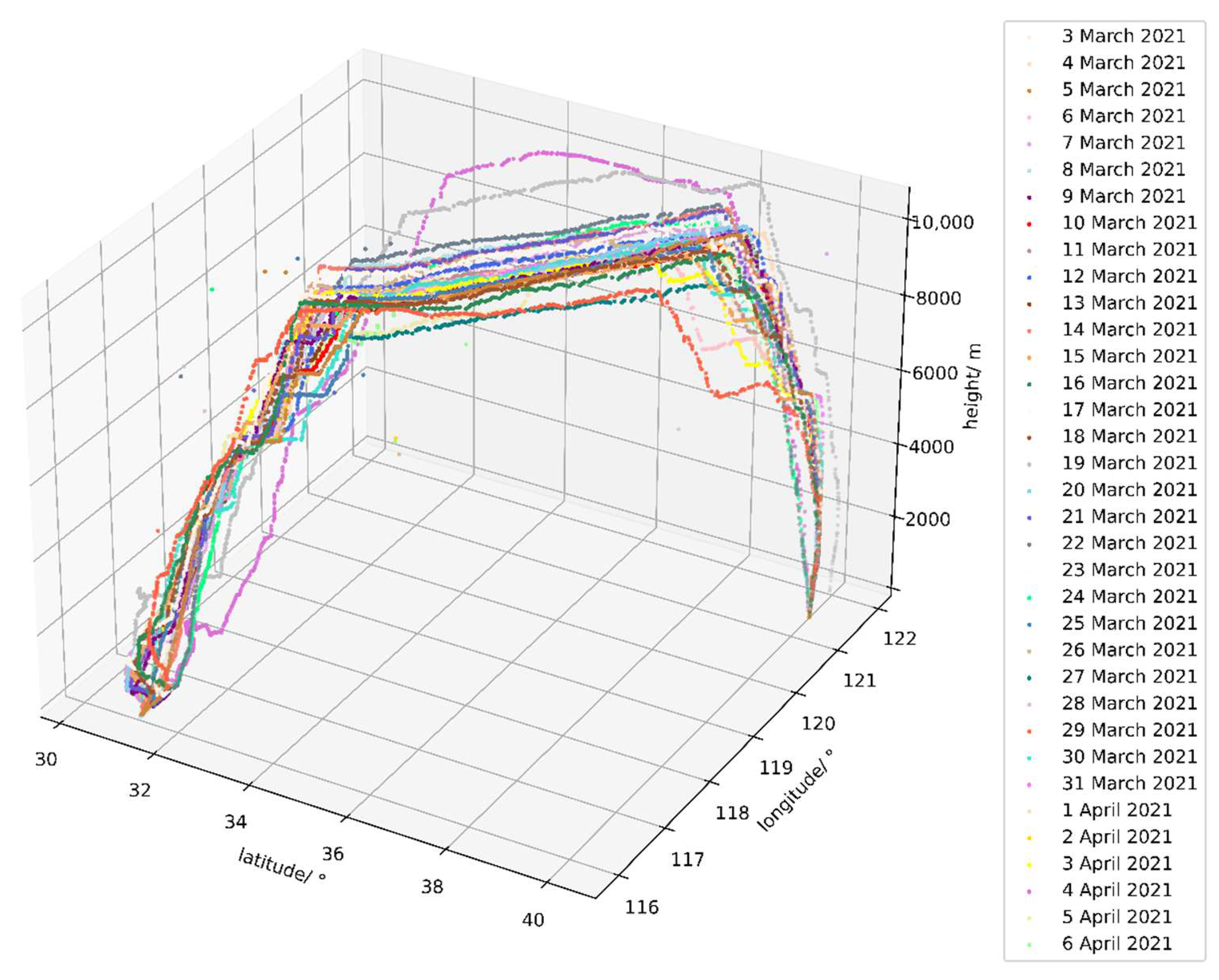
The experimental dataset used historical flight trajectory data from March 2021 to March 2022 on a real route, and some of the flight paths are shown in Figure 8.

4.2. Evaluation Index

The root mean square error (RMSE) and mean absolute error (MAE) are the most commonly used evaluation indices. The RMSE is the squared difference between the model result and the true and expected values of the square root. MAE is the difference between the model results and the true value mean of the absolute errors. The metrics are calculated according to Equations (24) and (25).
R M S E = [ 1 N j = 1 n ( Y j X j ) 2 ] 1 2
M A E = 1 N 1 n | Y j X j | ,
where N is the number of samples; Y j is the predicted trajectory; X j is the actual flight path. The smaller the value, the closer it is to the true value, which indicates a higher prediction accuracy of the model.

4.3. Calibration of the Model Parameter

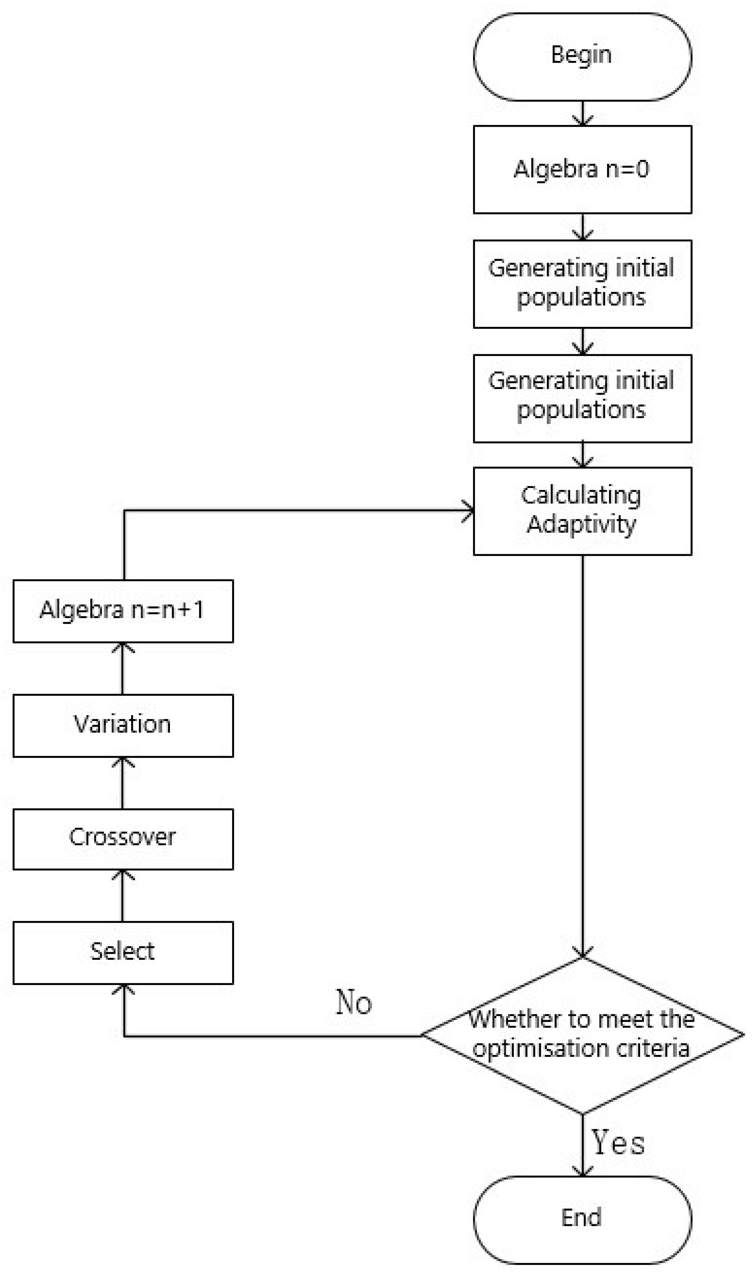
The basic principle of GA lies in modelling various potential solutions, where the initial individuals in the solution are generated randomly. The GA performs selection, crossover, and mutation operations on each individual to search for the optimal solution, thereby continuously generating solutions that approximate the true value until a certain number of new generations of individuals are generated, and the objective function is recalculated, with the best-performing individuals retained for the next generation based on their fitness. As each generation reproduces, the fitness function of the entire population decreases until it is impossible to improve the results. The flowchart of GA optimisation is shown in Figure 9.
(1)
Optimisation parameters: According to the DA-CNN-BiLSTM prediction model, the neural network parameters to be optimised include the number, size, and stride of the convolutional kernels of the two-layer CNN, the number of neurons of the two-layer BiLSTM, as well as the dropout rate and learning rate.
(2)
Objective function: The function Euclidean distance is as shown in Equation (26).
d = 1 n ( x 1 x 2 ) 2 + ( y 1 y 2 ) 2 + ( z 1 z 2 ) 2 ,
where d is the Euclidean distance between two waypoints; n is the sample size; x 1 and x 2 are the latitudes; y 1   a n d   y 2 are the longitudes; z 1 and z 2 are the altitudes.
(3)
Range of parameters: 1 c 1 60 , 1 n 1 3 , 1 s 1 2.99 , 1 b 1 100 , 1 c 2 60 , 1 n 2 3 , 1 s 2 2.99 , 1 b 2 100 , 0.1 d 0.9 , 10 4 l 10 2
where c 1 and c 2 are the numbers of convolutional kernels; n 1 and n 2 are the sizes of convolutional kernels; s 1 and s 2 are the strides of convolutional kernels; b 1 and b 2 are the numbers of BiLSTM neurons; d is the dropout rate; l is the learning rate.
(4)
GA parameters: Population size = 20, DNA length = 40, mutation rate = 0.01, max iteration = 5.
After the GA hyperparameter search, the prediction model structure was finally established, as shown in Table 2, and the error variation of the optimised model is shown in Figure 10. The error plot shows that the model performs well in the training and test datasets, and with an increase in the number of training generations, the error eventually oscillates smoothly around 0, indicating that the model has a strong generalisation capability.

4.4. Experiments and Comparison

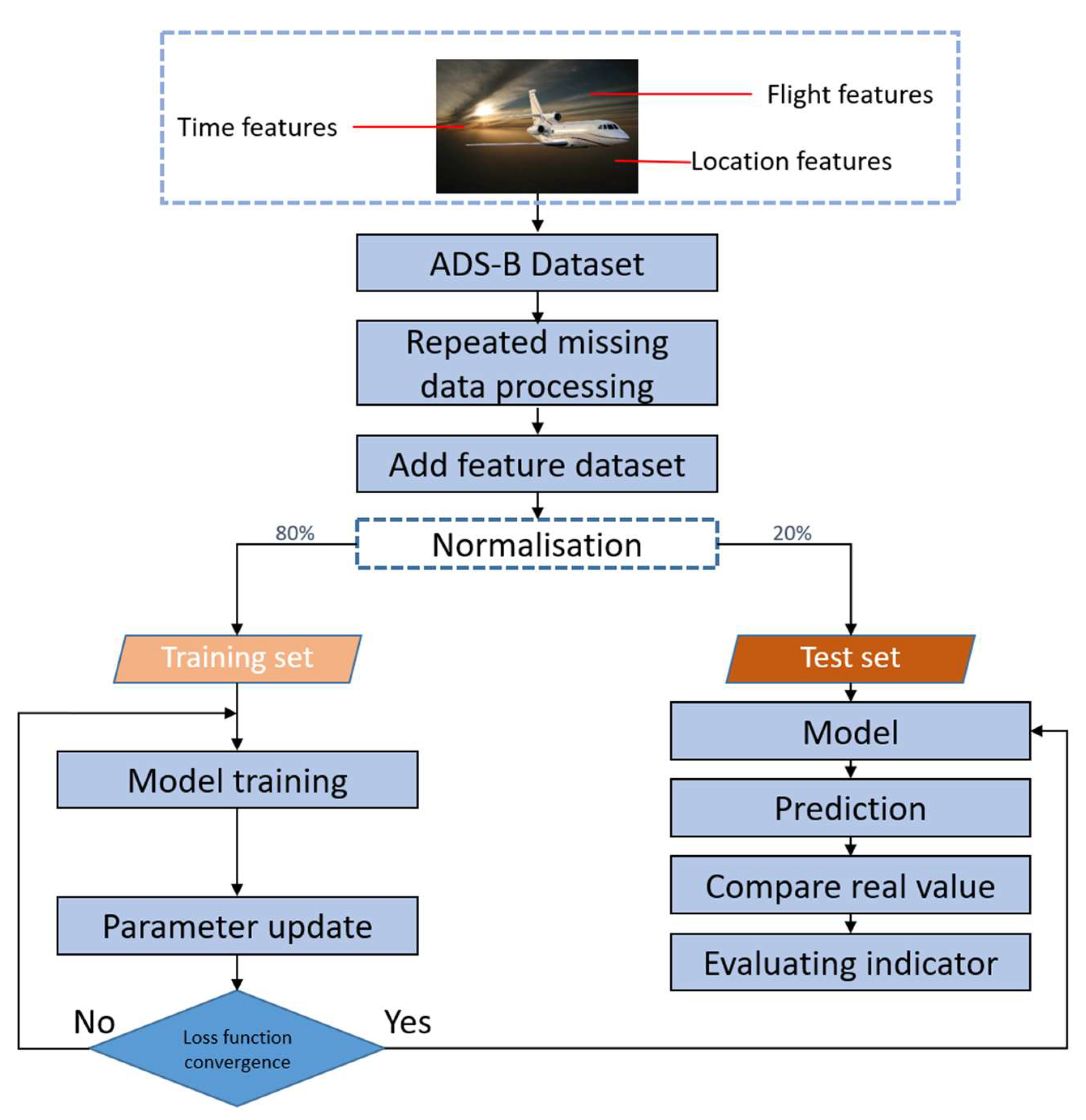
To test the prediction accuracy of the different models, their feasibility and accuracy were verified by simulation with a real ADS-B historical trajectory dataset. The proportion of the training and test sets impacts the modelling accuracy, as the model struggles to adequately reflect the nonlinear fit between the trajectory features and the predicted results when the training set is small. The proportion of the test set decreases when the training set is large, making it difficult for the test accuracy of the model to reflect accurate prediction accuracy. The size of the original dataset likely influences the determination of the training test set ratio. For example, a more extensive dataset should ensure that the model achieves high training and testing accuracy even with a more significant proportion of the training set. In this paper, the training set is chosen from {6:4, 7:3, 7.5:2.5, 8:2, 8.5:1.5, 9:1} and the results are shown in Figure 11. When the ratio is 8:2, prediction accuracy (RMSE) reaches its nadir, and it begins to rise and eventually becomes stable. The experimental procedure is illustrated in Figure 12.
First, we preprocessed the ADS-B trajectory data and trained them through a set network. The simulations were then validated, and the predicted trajectories were compared with the actual trajectories. The model was trained to reduce the error to a set range, after which it was tested with a test set.

4.4.1. Experimental Results

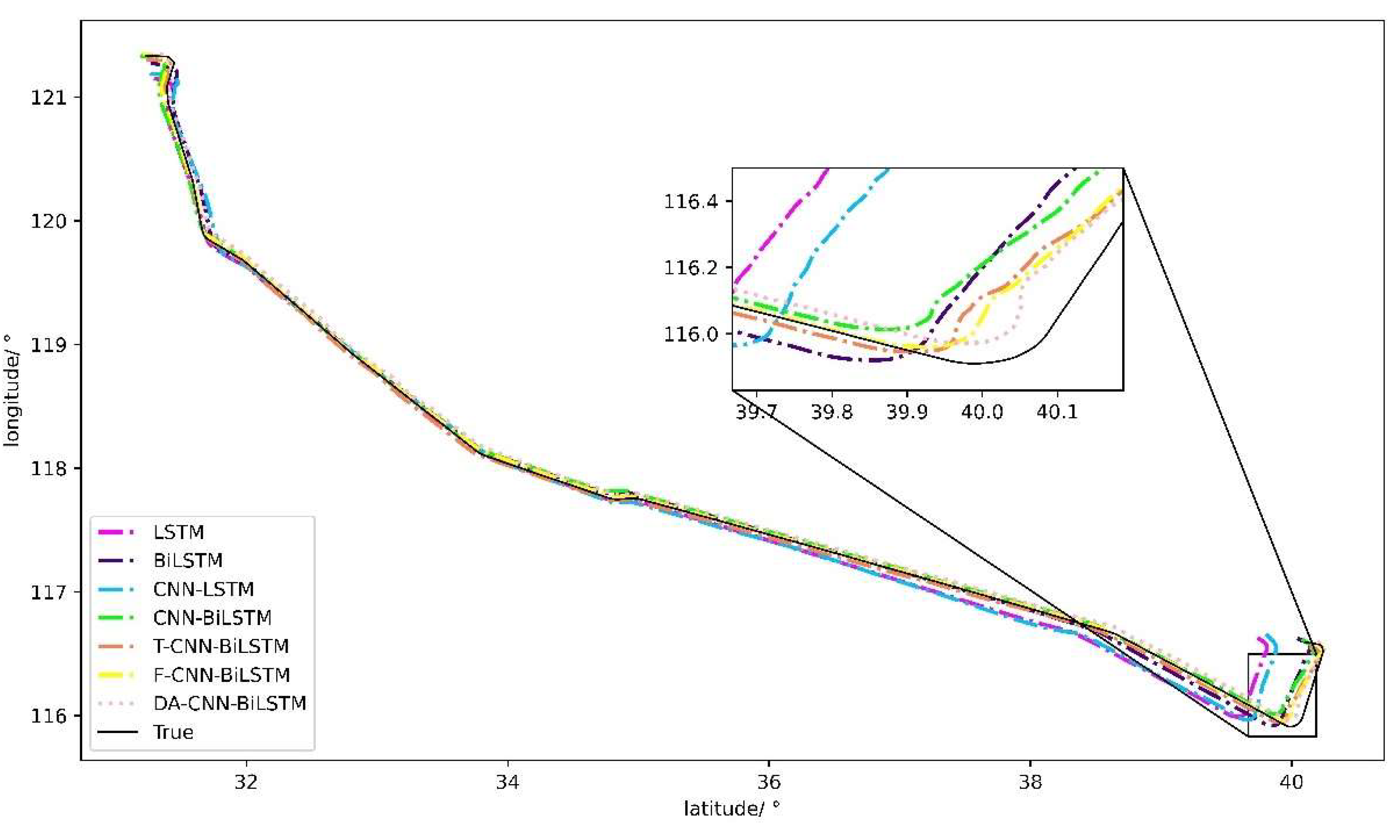
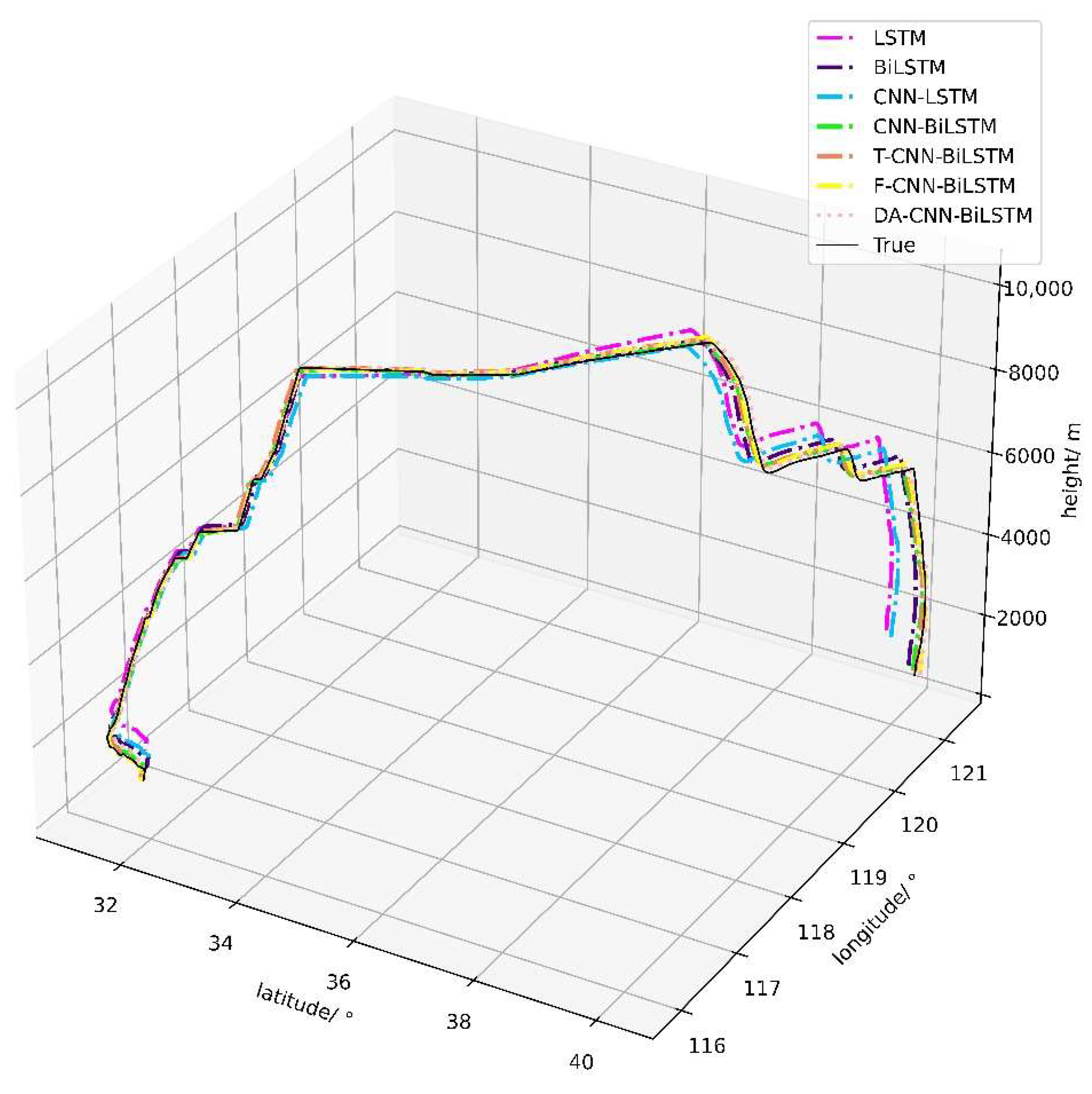
To validate the performance of the models better, all models (BiLSTM, LSTM, CNN-LSTM, CNN-BiLSTM, T-CNN-BiLSTM, F-CNN-BiLSTM, and DA-BiLSTM) were based on the same dataset for trajectory prediction. The results are presented in Table 3 and Figure 13. To illustrate the differences between the models more visually, two-dimensional zoomed-in and three-dimensional comparison plots of the prediction results are shown in Figure 13 and Figure 14.
The results confirm that the DA-CNN-BiLSTM has the best performance in trajectory prediction, with the lowest RMSE of 50.68 m and MAE of 32.37 m for altitude, the lowest RMSE of 0.029° and MAE of 0.022° for latitude, and the lowest RMSE of 0.018° and MAE of 0.014° for longitude. It can also be observed from Figure 14 and Figure 15 that the predicted trajectory of the DA-CNN-BiLSTM model best matches the actual trajectory, with a lower prediction error than the other models, specifically for large altitude changes and turning trajectory points.

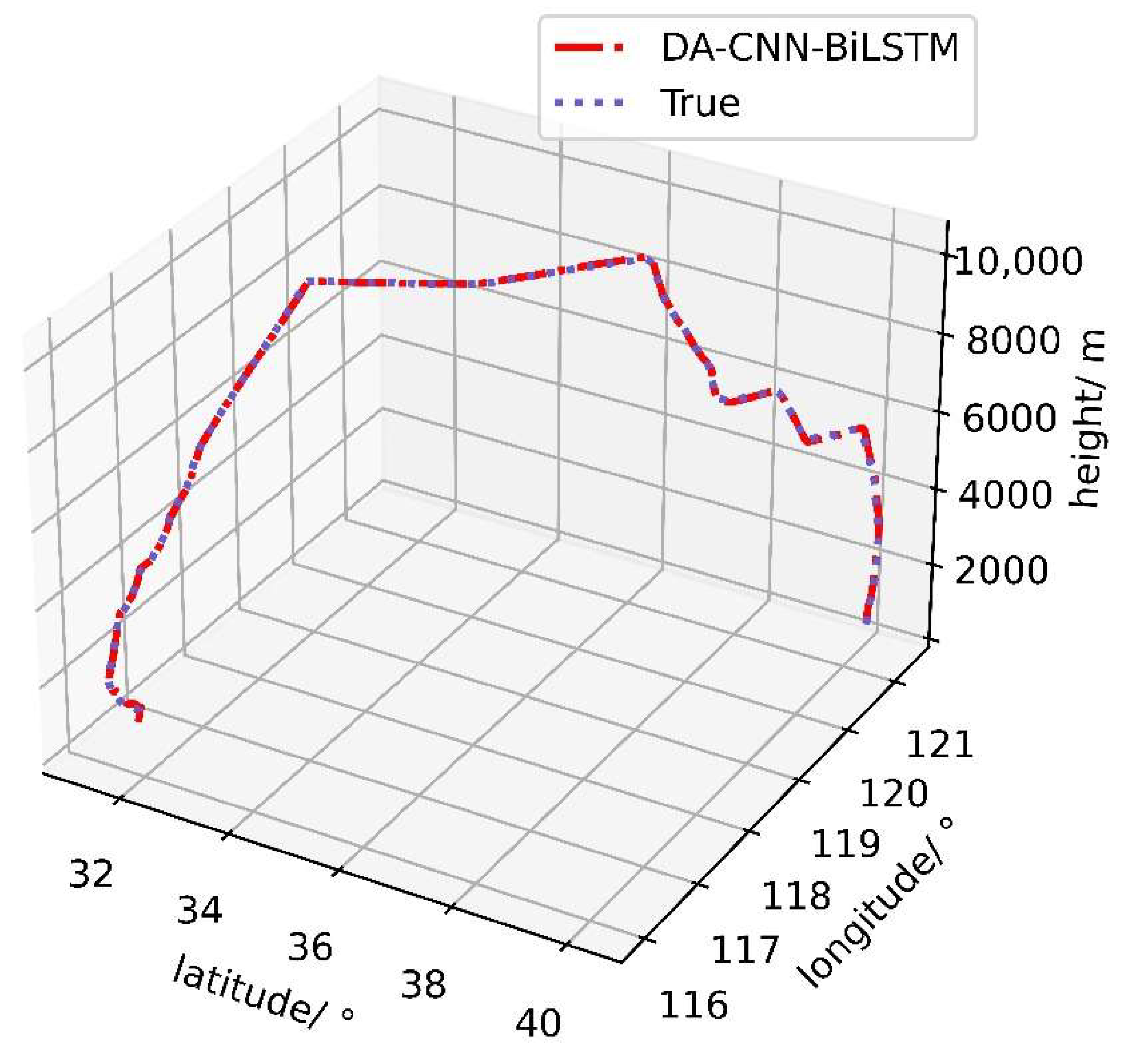
4.4.2. Comparative Analysis

Three sets of comparisons were made to further analyse the predicted results. The improvement ratios for the different models were introduced in Equation (27) to quantify the differences. First, a first set of comparisons was performed to account for the different effects of feature attention and temporal attention on the hybrid model. Second, to understand the importance of convolutional neural networks in extracting trajectory features better, a second set of comparisons was performed. Finally, to better analyse the significance of the BiLSTM model for extracting bidirectional temporal features, a third set of comparisons was performed. The three sets of comparisons are presented in Table 4.
I R ( i ) = | B ( i ) A ( i ) | / A ( i ) ,
where I R ( i ) is the rate of improvement of B compared with A using i as an indicator. A ( i ) and B ( i ) are the values of models A and B on indicator i , respectively. We used RMSE and MAE as indicators, where the smaller the predictive performance of the I R ( i ) model, the better.
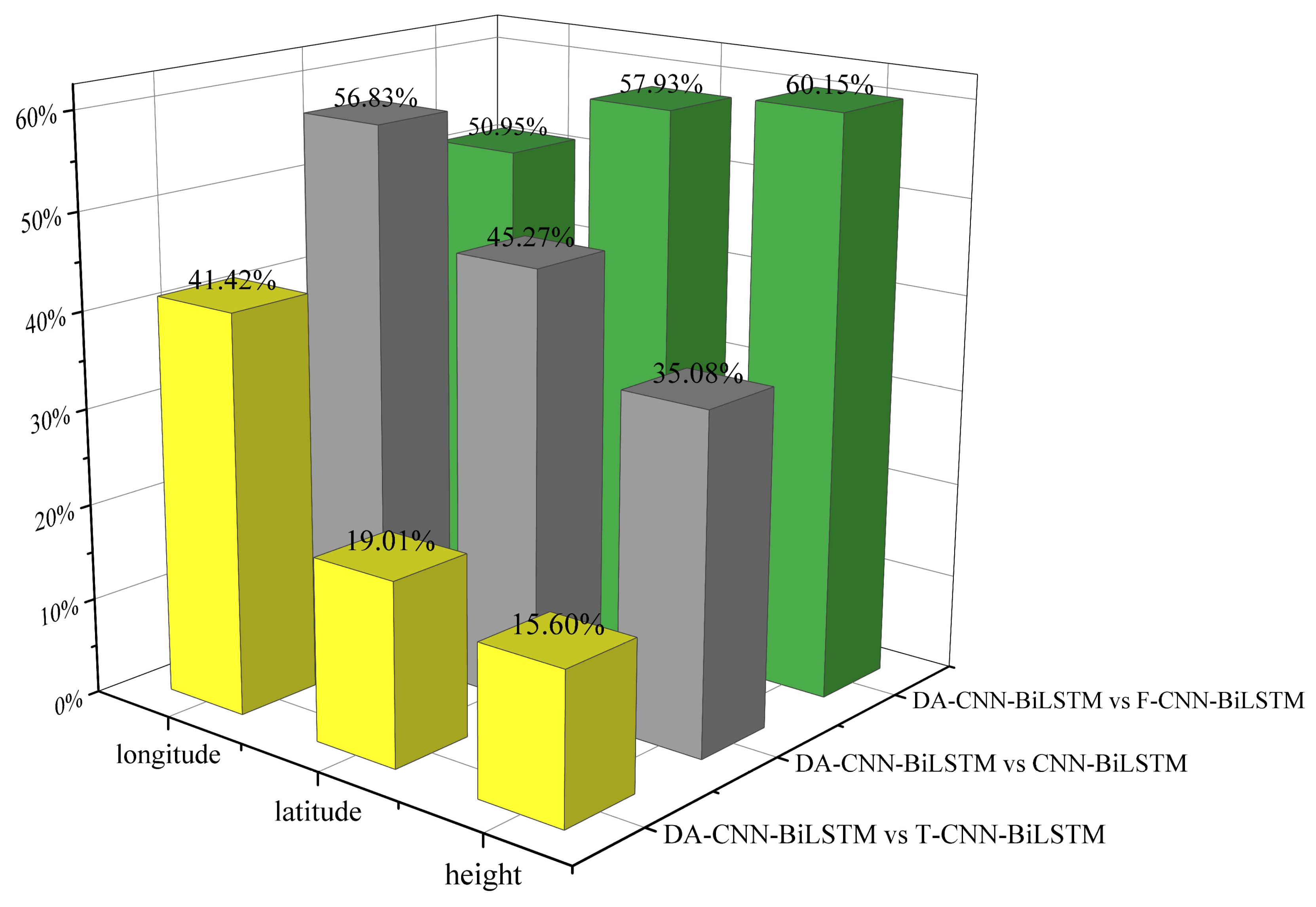
To compare the different effects of feature attention and temporal attention on the hybrid models in trajectory prediction, the following model comparison groups were introduced: DA-CNN-BiLSTM vs. T-CNN-BiLSTM, DA-CNN-BiLSTM vs. F-CNN-BiLSTM, and DA-CNN-BiLSTM vs. CNN-BiLSTM. The results are presented in Figure 16. We can observe that among the three sets of models, DA-CNN-BiLSTM had the best prediction performance and the lowest RMSE with a height of 50.68 m, longitude of 0.018°, and latitude of 0.029°.
Compared with F-CNN-BiLSTM, the RMSE improvement rates for DA-CNN-BiLSTM were 50.95%, 57.93%, and 60.15% for longitude, latitude, and altitude. Compared with T-CNN-BiLSTM, the RMSE improvement rates for DA-CNN-BiLSTM were 41.42%, 19.01%, and 15.60% for longitude, latitude, and altitude. The RMSE improvement rates for DA-CNN-BiLSTM were 56.83%, 45.27%, and 35.08% for longitude, latitude, and altitude, as compared to that of the CNN-BiLSTM without the attention model. We can conclude that DA-CNN-BiLSTM models have higher accuracy than the single attentional model and they have a lower operational error than the unattended model. In summary, the ability of the DA-CNN-BiLSTM to extract trajectory characteristics from the data and extract temporal features more effectively is important for improving the accuracy of short-term trajectory prediction.
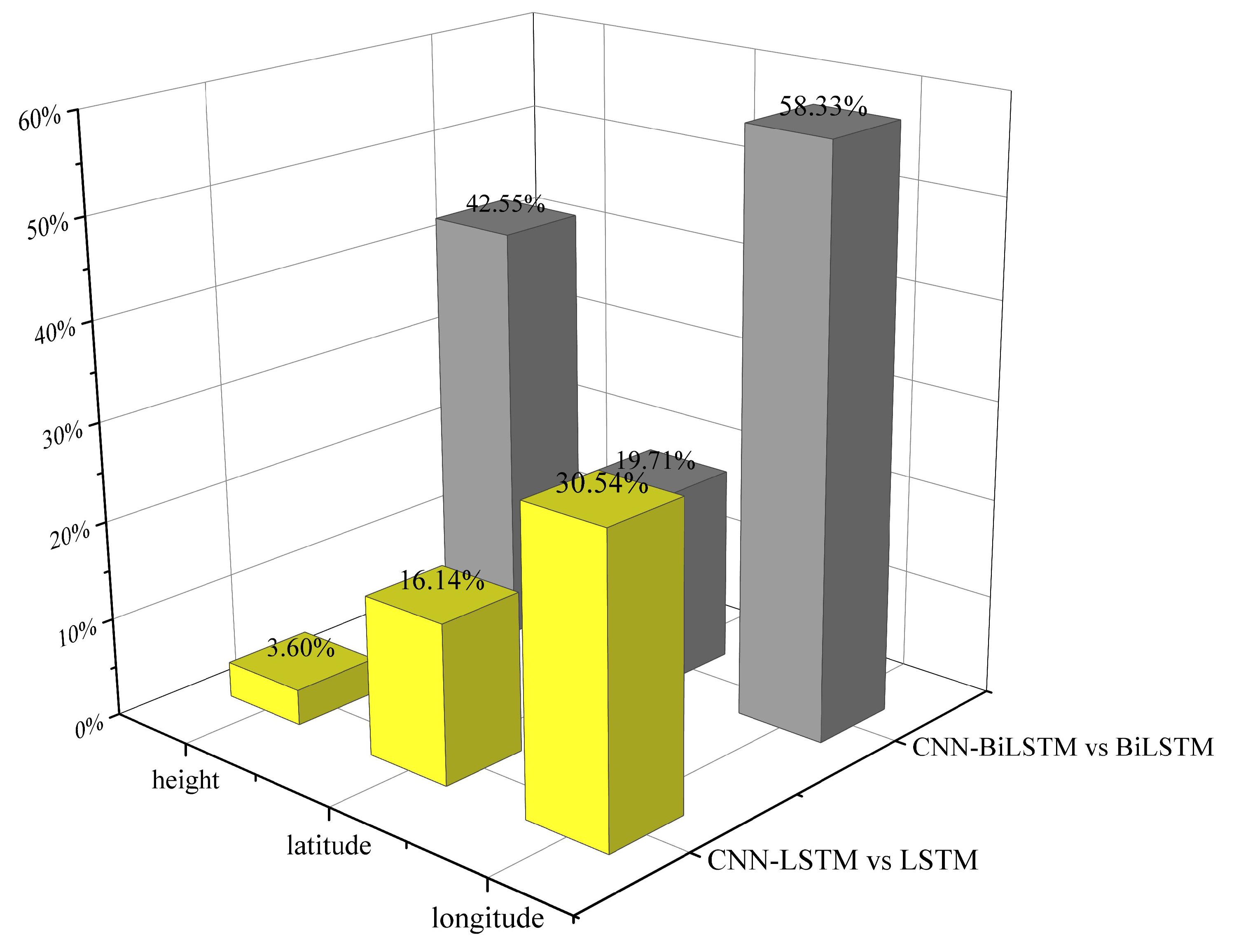
To better verify the importance of CNN in extracting trajectory features for prediction, we set up two sets of models for comparison: CNN-BiLSTM vs. BiLSTM and CNN-LSTM vs. LSTM. The results are presented in Figure 17. In the two model comparison groups, CNN-BiLSTM had the best performance and the lowest RMSE, with a height of 87.96 m, longitude of 0.043°, and latitude of 0.078°. The combined CNN model has a higher prediction accuracy than the BiLSTM and LSTM single models.
Compared with the single-model BiLSTM, the RMSE improvement rates for CNN-BiLSTM were 42.55%, 19.71%, and 58.83% for longitude, latitude, and altitude. Compared to the single-model LSTM, the RMSE improvement rates for CNN-LSTM were 3.6%, 16.14%, and 30.54% for longitude, latitude, and altitude. We can observe that the model with the CNN has higher accuracy. In summary, the CNN’s ability to extract spatial features from different trajectory points is particularly effective and important for improving the accuracy of short-term trajectory prediction.
To verify the importance of the BiLSTM bidirectional extraction of temporal features of the trajectory in prediction, we set up two sets of models for comparison: BiLSTM vs. LSTM and CNN-BiLSTM vs. CNN-LSTM. The results are presented in Figure 18.
In contrast to the LSTM model, there were RMSE improvements of 53.08%, 37.04%, and 57.53% for longitude, latitude, and altitude for BiLSTM. Compared to the CNN-LSTM model, the RMSE improvement rates for CNN-BiLSTM were 72.04%, 56.47%, and 74.83% for longitude, latitude, and altitude. We can observe that the BiLSTM and its hybrid models can play a better role in trajectory prediction than ordinary LSTM models because BiLSTM can mine the trajectory temporal features from front to back and from back to front.

4.5. Further Research

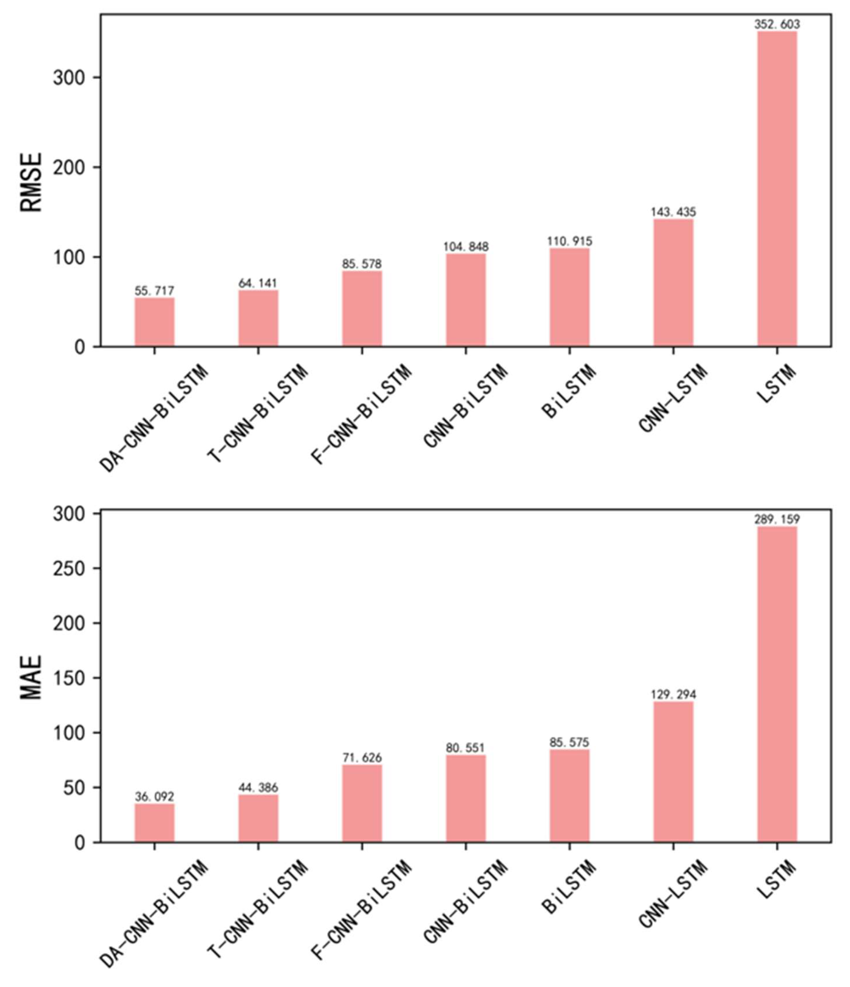
To analyse and validate the robustness and generality of the DA-CNN-BiLSTM model based on the dual attention mechanism under different data conditions, a dataset of another flight on the same route was selected for testing, with data ranging from May 2021 to May 2022. The entire dataset was used for 80% of the training set and 20% of the test set for training optimisation and testing, respectively. The proposed prediction model, DA-CNN-BiLSTM, as well as other models (DA-CNN-BiLSTM, F-CNN-BiLSTM, T-CNN-BiLSTM, CNN-BiLSTM, CNN-LSTM, BiLSTM, and LSTM) were optimised using GA to determine the model hyperparameter, and they were trained using this dataset; the prediction results and evaluation index are shown in Figure 19 and Figure 20.
As shown in Figure 18 and Figure 19, the prediction curves of the proposed DA-CNN-BiLSTM model were generally consistent with the actual routes. Compared to the other comparative models, the RMSE and MAE were the lowest. The DA-CNN-BiLSTM model performed better in terms of prediction accuracy. The DA-CNN-BiLSTM based on the dual attention mechanism can achieve higher accuracy and robustness in the trajectory prediction problem.

5. Conclusions and Discussion

In this study, DA-CNN-BiLSTM was proposed for trajectory prediction. Specifically, a hybrid network of convolutional neural networks and feature attention modules was constructed which can effectively learn spatial structural features in the trajectory without requiring information about aircraft-specific parameters. Additionally, a BiLSTM neural network with temporal attention module network, which fully exploits the aircraft historical time-series information, was constructed, followed by optimisation of the model hyperparameter by GA to predict the trajectory information effectively. We demonstrated that the DA-CNN-BiLSTM model with the addition of feature attention and temporal attention mechanisms could improve the longitude, latitude, and height prediction performance by 56.83%, 45.27%, and 35.08%. In summary, the DA-CNN-BiLSTM model offers higher accuracy and adaptability in the trajectory prediction process than conventional models. The prediction process only uses the ADS-B historical trajectory, which requires less information. At the same time, the key element of the TBO operation consists of the controller’s situational awareness of the aircraft, which in turn depends on how well the controller can predict aircraft operations, specifically, the future position of all aircraft. Therefore, accurate and reliable aircraft trajectory forecasting is valuable for conflict detection relief, traffic management, flight sequencing, and arrival management. The framework will be improved in the future by selecting additional evaluation metrics and implementing long-term forecasts.

Author Contributions

Conceptualization, J.H. and W.D.; methodology, W.D.; software, W.D.; validation, G.S., J.H., and X.W.; formal analysis, J.H.; investigation, B.L.; resources, X.W.; data curation, W.D.; writing—original draft preparation, W.D.; writing—review and editing, J.H.; visualization, G.S.; supervision, Y.L.; project administration, J.H.; funding acquisition, H.L. All authors have read and agreed to the published version of the manuscript.

Funding

This study was co-supported by the CAAC Vertical Project (Project No. 0242021), the Civil Aviation Air Traffic Management Authority Horizontal Project (Project No. 0052119 and Project No. 0052154), and the Institute of New Technologies for Civil Aviation Communications Navigation Surveillance (Project No. JG202220).

Institutional Review Board Statement

Not applicable.

Informed Consent Statement

Not applicable.

Data Availability Statement

Data available on request due to restrictions, e.g., privacy or ethical.

Conflicts of Interest

The authors declare no conflict of interest.

References

  1. Mondoloni, S.; Rozen, N. Aircraft Trajectory Prediction and Synchronization for Air Traffic Management Applications. Prog. Aerosp. Sci. 2020, 119, 100640. [Google Scholar] [CrossRef]
  2. Sahadevan, D.; Ponnusamy, P.; Gopi, V.P.; Nelli, M.K. Ground-based 4d trajectory prediction using bi-directional LSTM networks. Appl. Intell. 2022, 32, 1–18. [Google Scholar] [CrossRef]
  3. Rosenow, J.; Fricke, H. Impact of multi-criteria optimized trajectories on European airline efficiency, safety and airspace demand. J. Air Transp. Manag. 2019, 78, 133–143. [Google Scholar] [CrossRef]
  4. Li, X.; Yan, H.; Zhang, Y. Optimization of Multisource Dynamic Model in TBO. Math. Probl. Eng. 2022, 2022, 3755574. [Google Scholar] [CrossRef]
  5. Zeng, W.; Chu, X.; Xu, Z.; Liu, Y.; Quan, Z. Aircraft 4D Trajectory Prediction in Civil Aviation: A Review. Aerospace 2022, 9, 91. [Google Scholar] [CrossRef]
  6. Hashemi, S.M.; Botez, R.M.; Grigorie, T.L. New Reliability Studies of Data-Driven Aircraft Trajectory Prediction. Aerospace 2020, 7, 145. [Google Scholar] [CrossRef]
  7. Zhang, J.; Ge, T.; Chen, Q.; Wang, F. 4D Trajectory Prediction and Uncertainty Analysis for Departure Aircraft. J. Southwest Jiaotong Univ. 2016, 51, 800–806. [Google Scholar]
  8. He, D.Y. Research on Aircraft Trajectory Planning Based on Centralised Flight Plan Processing. Master’s Thesis, Civil Aviation Flight Academy of China, Chengdu, China, 2020. [Google Scholar]
  9. Kang, N.; Han, X.; Hu, Y.; Wei, Z. Departure aircraft altitude profile prediction based on aircraft mass estimation strategy. J. Civ. Aviat. Univ. China 2019, 37, 11–16. [Google Scholar]
  10. Lee, J.; Lee, S.; Hwang, I. Hybrid System Modeling and Estimation for Arrival Time Prediction in Terminal Airspace. J. Guid. Control. Dyn. 2016, 39, 903–910. [Google Scholar] [CrossRef]
  11. Chen, M.; Fu, J. Flight Track Prediction Method Based on Unscented Kalman Filter. Comput. Simul. 2021, 38, 27–30+36. [Google Scholar]
  12. Lv, B.; Wang, C. Application of improved extended Kalman filtering in aircraft 4D trajectory prediction algorithm. J. Comput. Appl. 2021, 277–282. [Google Scholar]
  13. Zhou, J.; Zhang, H.; Lyu, W.; Wan, J.; Zhang, J.; Song, W. Hybrid 4-Dimensional Trajectory Prediction Model, Based on the Reconstruction of Prediction Time Span for Aircraft en Route. Sustainability 2022, 14, 3862. [Google Scholar] [CrossRef]
  14. Tang, X.; Zheng, P. IMM aircraft short-term track extrapolation based on geodetic coordinate system. Syst. Eng. Electron. 2022, 44, 2293–2301. [Google Scholar]
  15. Sighencea, B.I.; Stanciu, R.I.; Caleanu, C.D. A Review of Deep Learning-Based Methods for Pedestrian Trajectory Prediction. Sensors 2021, 21, 7543. [Google Scholar] [CrossRef] [PubMed]
  16. Zhang, Z.; Ni, G.; Xu, Y. Ship Trajectory Prediction Based on LSTM Neural Network. In Proceedings of 2020 IEEE 5th Information Technology and Mechatronics Engineering Conference (itoec 2020), Chongqing, China, 12–14 June 2020; Xu, B., Mou, K., Eds.; IEEE: New York, NY, USA, 2020; pp. 1356–1364. [Google Scholar]
  17. Karimzadeh, M.; Aebi, R.; de Souza, A.M.; Zhao, Z.; Braun, T.; Sargento, S.; Villas, L. Reinforcement Learning-Designed LSTM for Trajectory and Traffic Flow Prediction. In Proceedings of the 2021 IEEE Wireless Communications and Networking Conference (WCNC), Nanjing, China, 29 March 2021; pp. 1–6. [Google Scholar]
  18. Han, P.; Wang, W.; Shi, Q.; Yue, J. A Combined Online-Learning Model with K-Means Clustering and GRU Neural Networks for Trajectory Prediction. Ad Hoc Netw. 2021, 117, 102476. [Google Scholar] [CrossRef]
  19. Madar, S.; Puranik, T.G.; Mavris, D.N. Application of Trajectory Clustering for Aircraft Conflict Detection. In Proceedings of the 2021 IEEE/AIAA 40th Digital Avionics Systems Conference (DASC), San Antonio, TX, USA, 3 October 2021; pp. 1–9. [Google Scholar]
  20. Yin, Y.; Tong, M. Application of GRIB Data for 4D Trajectory Prediction. In Proceedings of the Artificial Intelligence in China; Liang, Q., Wang, W., Mu, J., Liu, X., Na, Z., Chen, B., Eds.; Springer: Singapore, 2020; pp. 422–430. [Google Scholar]
  21. Pang, Y.; Xu, N.; Liu, Y. Aircraft Trajectory Prediction Using LSTM Neural Network with Embedded Convolutional Layer. Annu. Conf. PHM Soc. 2019, 11, 11. [Google Scholar] [CrossRef]
  22. Liu, L.; Zhai, L.; Han, Y. Aircraft trajectory prediction based on conv LSTM. Comput. Eng. Des. 2022, 43, 1127–1133. [Google Scholar] [CrossRef]
  23. Shi, Q.; Wang, W.; Han, P. Short-term 4D Trajectory Prediction Algorithm Based on Online-updating LSTM Network. J. Signal Process. 2021, 37, 66–74. [Google Scholar] [CrossRef]
  24. Zeng, W.; Quan, Z.; Zhao, Z.; Xie, C.; Lu, X. A Deep Learning Approach for Aircraft Trajectory Prediction in Terminal Airspace. IEEE Access 2020, 8, 151250–151266. [Google Scholar] [CrossRef]
  25. Han, P.; Yue, J.; Fang, C.; Shi, Q.; Yang, J. Short-Term 4D Trajectory Prediction Based on LSTM Neural Network. In Proceedings of the Second Target Recognition and Artificial Intelligence Summit Forum; Wang, T., Chai, T., Fan, H., Yu, Q., Eds.; SPIE: Changchun, China, 2020; p. 23. [Google Scholar]
  26. Shi, Z.; Xu, M.; Pan, Q.; Yan, B.; Zhang, H. LSTM-Based Flight Trajectory Prediction. In Proceedings of the 2018 International Joint Conference on Neural Networks (IJCNN), Rio de Janeiro, Brazil, 8–13 July 2018; pp. 1–8. [Google Scholar]
  27. Yang, K.; Bi, M.; Liu, Y.; Zhang, Y. LSTM-based deep learning model for civil aircraft position and attitude prediction approach. In Proceedings of the 2019 Chinese Control Conference (CCC), Guangzhou, China, 27–30 July 2019; pp. 8689–8694. [Google Scholar]
  28. Xu, Z.; Zeng, W.; Chu, X.; Cao, P. Multi-Aircraft Trajectory Collaborative Prediction Based on Social Long Short-Term Memory Network. Aerospace 2021, 8, 115. [Google Scholar] [CrossRef]
  29. Ma, L.; Tian, S. A Hybrid CNN-LSTM Model for Aircraft 4D Trajectory Prediction. IEEE Access 2020, 8, 134668–134680. [Google Scholar] [CrossRef]
  30. Hu, D.; Meng, X.; Lu, S.; Xing, L. Parallel LSTM-FCN Model Applied to Vessel Trajectory Prediction. Control Decis. 2022, 37, 1–7. [Google Scholar] [CrossRef]
  31. Manesh, M.R.; Kaabouch, N. Analysis of Vulnerabilities, Attacks, Countermeasures and Overall Risk of the Automatic Dependent Surveillance-Broadcast (ADS-B) System. Int. J. Crit. Infrastruct. Prot. 2017, 19, 16–31. [Google Scholar] [CrossRef]
  32. Zhou, F.; Jin, L.; Dong, J. Review of convolutional neural network. Chin. J. Comput. 2017, 40, 1229–1251. [Google Scholar]
  33. Yu, Y.; Si, X.; Hu, C.; Zhang, J. A review of recurrent neural networks: LSTM cells and network architectures. Neural Comput. 2019, 31, 1235–1270. [Google Scholar] [CrossRef] [PubMed]
  34. Peng, Y.; Han, Q.; Su, F.; He, X.; Feng, X. Meteorological Satellite Operation Prediction Using a BiLSTM Deep Learning Model. Secur. Commun. Netw. 2021, 2021, 9916461. [Google Scholar] [CrossRef]
  35. Li, A.; Xiao, F.; Zhang, C.; Fan, C. Attention-based interpretable neural network for building cooling load prediction. Appl. Energy 2021, 299, 117238. [Google Scholar] [CrossRef]
  36. Meng, Q.; Shang, B.; Liu, Y.; Guo, H.; Zhao, X. Intelligent Vehicles Trajectory Prediction with Spatial and Temporal Attention Mechanism. In Proceedings of the Ifac Papersonline; Elsevier: Amsterdam, The Netherlands, 2021; Volume 54, pp. 454–459. [Google Scholar]
  37. Lin, Z.; Cheng, L.; Huang, G. Electricity Consumption Prediction Based on LSTM with Attention Mechanism. IEEJ Trans. Electr. Electron. Eng. 2020, 15, 556–562. [Google Scholar] [CrossRef]
  38. He, X.; He, Z.; Song, J.; Liu, Z.; Jiang, Y.-G.; Chua, T.-S. Nais: Neural attentive item similarity model for recommendation. IEEE Trans. Knowl. Data Eng. 2018, 30, 2354–2366. [Google Scholar] [CrossRef] [Green Version]
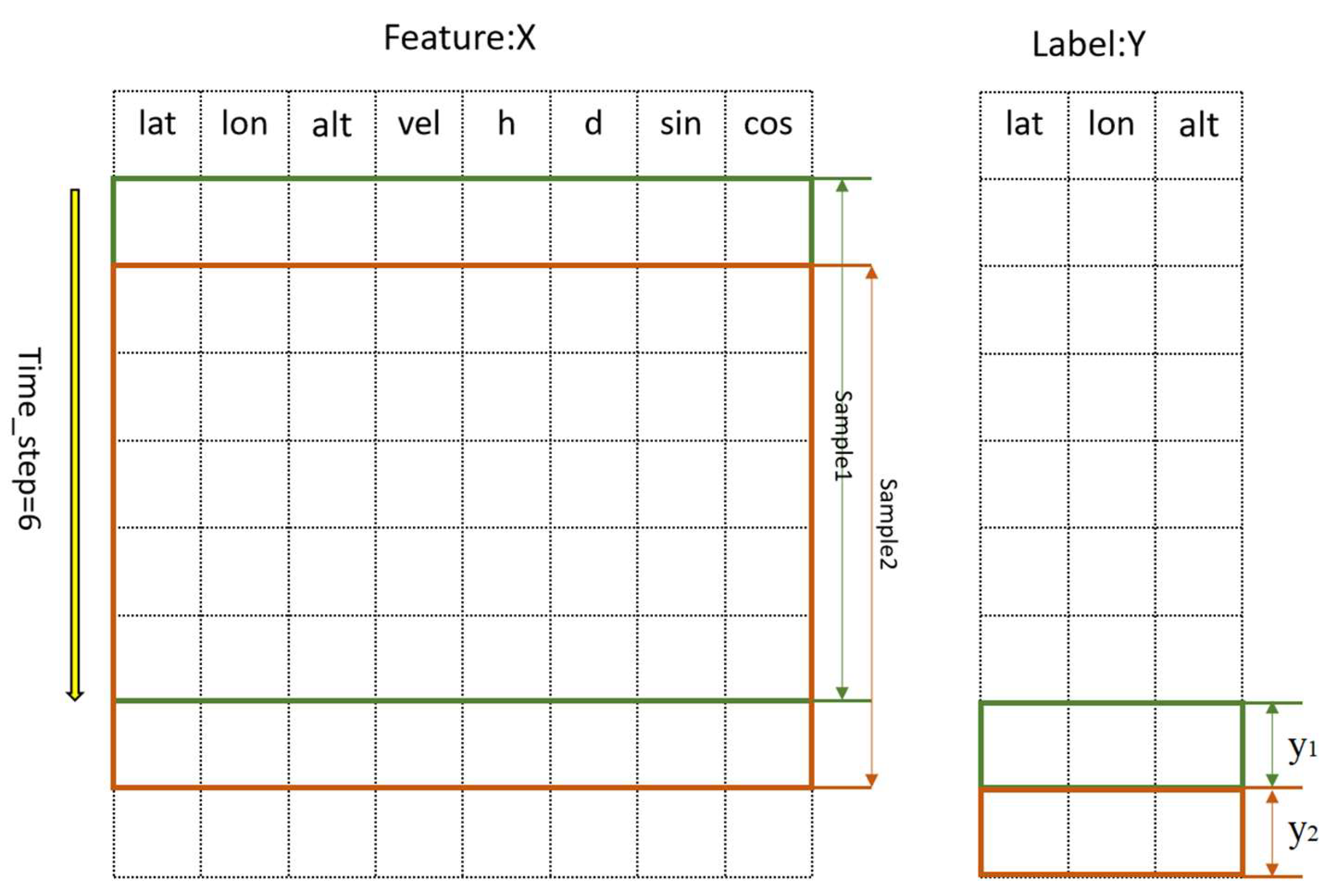
Figure 1. Illustration of sample splitting.
Aerospace 09 00464 g001
Figure 2. Structure of the CNN.
Aerospace 09 00464 g002
Figure 3. Structure of the LSTM.
Aerospace 09 00464 g003
Figure 4. Structure of the BiLSTM.
Aerospace 09 00464 g004
Figure 5. Feature attention mechanism.
Aerospace 09 00464 g005
Figure 6. Time attention mechanism.
Aerospace 09 00464 g006
Figure 7. Architecture of the DA-CNN-BiLSTM hybrid model.
Aerospace 09 00464 g007
Figure 8. Trajectory dataset.
Aerospace 09 00464 g008
Figure 9. Genetic algorithm (GA) flow chart.
Aerospace 09 00464 g009
Figure 10. Optimised neural network model error.
Aerospace 09 00464 g010
Figure 11. The influence of training set and test set partitioning on prediction accuracy. Effect of prediction accuracy.
Aerospace 09 00464 g011
Figure 12. Experimental procedure.
Aerospace 09 00464 g012
Figure 13. Prediction result.
Aerospace 09 00464 g013
Figure 14. Prediction comparison with 2D.
Aerospace 09 00464 g014
Figure 15. Prediction comparison with 3D.
Aerospace 09 00464 g015
Figure 16. Results of the 1st set of comparison.
Aerospace 09 00464 g016
Figure 17. Results of the 2nd set of comparison.
Aerospace 09 00464 g017
Figure 18. Results of the 3rd set of comparison.
Aerospace 09 00464 g018
Figure 19. Predicted results and actual trajectory.
Aerospace 09 00464 g019
Figure 20. Comparison of the multi-model evaluation indicators.
Aerospace 09 00464 g020
Table 1. Trajectory point attribute.
FeatureTrajectory Point
Time4 March 20211 3: 38: 22
AnumB5372
ForumHU7603
Longitude/(°)116.26586
Latitude/(°)39.37152
Altitude/(m)8610.61
Velocity/(km/h)890.81
Angle/(°)156
Distance/(m)1,016,975.48
sin θ −0.333
cos θ 0.943
Table 2. Model parameter settings.
Model
DA-CNN-BiLSTMCNNConvolutionFilter = 50;
Kernel size = 3;
Stride = 1;
Epochs = 100;
Batch size = 256;
Optimiser =
‘Adam’;
Learning rate =
0.002591
Max-poolingKernel size = 2;
Stride = 1;
ConvolutionFilter = 50;
Kernel size = 2;
Stride = 1;
Max-poolingKernel size = 2;
Stride = 1;
F-Attention-Layer
BiLSTMUnits1Units80
Dropout0.2493
Units2Units90
Dropout0.2493
T-Attention-Layer
OutputDense3
Table 3. Comparative results of evaluation indicators.
RMSE
Hybrid ModelSingle
Model
DA-CNN-BiLSTMT-CNN-BiLSTMF-CNN-BiLSTMCNN-BiLSTMCNN-LSTMBiLSTMLSTM
Alt/(m)50.6860.05127.1778.07310.13189.64446.52
Lat/(°)0.0290.0360.0690.0430.1890.0920.196
Lon/(°)0.0180.0310.0380.0530.0980.0530.084
MAE
Hybrid ModelSingle
Model
DA-CNN-BiLSTMT-CNN-BiLSTMF-CNN-BiLSTMCNN-BiLSTMCNN-LSTMBiLSTMLSTM
Alt/(m)32.3738.35116.0660.27219.16151.13329.12
Lat/(°)0.0220.0270.0630.0330.1580.0810.128
Lon/(°)0.0140.0250.0330.0480.080.0450.059
Table 4. Multi-model comparison.
Details
1st set
comparison
DA-CNN-BiLSTM vs.
T-CNN-BiLSTM
DA-CNN-BiLSTM vs.
F-CNN-BiLSTM
DA-CNN-BiLSTM vs.
CNN-BiLSTM
2nd set
comparison
CNN-LSTM vs. LSTMCNN-BiLSTM vs.
BiLSTM
3rd set
comparison
BiLSTM vs. LSTMCNN-BiLSTM vs.
CNN-BiLSTM
Publisher’s Note: MDPI stays neutral with regard to jurisdictional claims in published maps and institutional affiliations.