Article

Forecasting Selected Commodities’ Prices with the Bayesian Symbolic Regression

by
Krzysztof Drachal
* and
Michał Pawłowski
Faculty of Economic Sciences, University of Warsaw, 00-241 Warszawa, Poland
*
Author to whom correspondence should be addressed.
Int. J. Financial Stud. 2024, 12(2), 34; https://doi.org/10.3390/ijfs12020034
Submission received: 18 December 2023 / Revised: 13 March 2024 / Accepted: 25 March 2024 / Published: 29 March 2024

Abstract

:
This study firstly applied a Bayesian symbolic regression (BSR) to the forecasting of numerous commodities’ prices (spot-based ones). Moreover, some features and an initial specification of the parameters of the BSR were analysed. The conventional approach to symbolic regression, based on genetic programming, was also used as a benchmark tool. Secondly, various other econometric methods dealing with variable uncertainty were estimated including Bayesian Model Averaging, Dynamic Model Averaging, LASSO, ridge, elastic net, and least-angle regressions, etc. Therefore, this study reports a concise and uniform comparison of an application of several popular econometric models to forecasting the prices of numerous commodities. Robustness checks and statistical tests were performed to strengthen the obtained conclusions. Monthly data beginning from January 1988 and ending in August 2021 were analysed.

1. Introduction

The objective of this paper is to apply a novel econometric tool in forecasting various commodities’ prices. The novelty of the applied method lies in its fusion of two distinct approaches: symbolic regression (Koza 1998) and Bayesian econometrics (Koop 2017). The rationale behind such an idea stems from the challenges faced by researchers when constructing forecasting models, particularly when selecting explanatory variables for methods such as multilinear regressions. This is a non-trivial task (Tapia Cortez et al. 2018), especially when adopting the (standard) frequentist approach and employing the commonly used ordinary least squares method to estimate regression coefficients.
Of course, there are some classical techniques available for selecting explanatory variables, but the issue of model uncertainty still remains a serious challenge. Researchers sometimes address this problem by using conventional tools such as model averaging techniques (Steel 2020; Burnham and Anderson 2002). However, applying the frequentist approach still requires careful analysis and is susceptible to human bias. Moreover, when dealing with data sets consisting of more variables than the number of observations, the Bayesian approach often becomes a useful alternative (Koop 2017).
Indeed, a viable solution to this issue is transitioning from the frequentist approach to the Bayesian one, which generally is an efficient tool in forecasting commodity prices (Nurmakhanova 2020). In the Bayesian framework, a researcher starts from some prior knowledge or assumptions on estimated coefficients, which are then updated with the new information forming the posterior knowledge. Such an approach offers several advantages. Mathematically, it enables dealing with a higher number of explanatory variables than observations for each time series. Moreover, it closely resembles the real-life market scenarios, in which investors can continuously update their econometric models with the new information in each session, re-estimating coefficients accordingly (Koop 2017).
In other words, the Bayesian approach starts with an initial (prior) belief about the parameter of interest. As the new information becomes available, this belief is updated, leading to the posterior belief. Consequently, a value of the parameter of interest evolves over time as this new information emerges. It is worth noting that these considerations not only apply to the technical challenge of selecting explanatory variables for regression models but are also valid for more complex models (Koop 2017).
Notably, the combination of symbolic regression with Bayesian principles has not been extensively explored yet, despite both approaches being philosophically well-suited to address real market problems, as already described (Jin et al. 2019). Thus, the proposed combination of these two formalisms represents an intriguing endeavour. This can introduce a new econometric tool and contribute to the ongoing scientific discourse surrounding model uncertainty and variable selection. Surprisingly, limited attempts to integrate these formalisms have been made yet (Vazquez et al. 2022; Guimera et al. 2020; Jin et al. 2019; Regolin and Pozo 2005; Zhang 2000).
Nevertheless, it should be noted that Bayesian methods are not always computationally “cheap” in this context (Lan et al. 2022). Moreover, in economics or finance, symbolic regression has not yet been extensively applied. There are some studies on forecasting production or emission quotas, but no application to price forecasting (Yang et al. 2015a, 2015b). Symbolic regression itself, which is a well-known tool (Koza 1998; Sinha et al. 2015), relies heavily on evolutionary algorithms, especially genetic ones (Koza 1998; Bhattacharya et al. 2016; Sinha et al. 2015; Eiben and Smith 2015).
Interestingly, genetic algorithms have been used in various econometric models, and were claimed to be very useful (Claveria et al. 2022; Garcia and Kristjanpoller 2019; Claveria et al. 2016, 2017; Mostafa and El-Masry 2016; Aguilar-Rivera et al. 2015; Sermpinis et al. 2015; Sheta et al. 2013; Hasheminia and Niaki 2006). While widely popular in technical fields, such as engineering, and nature-oriented sciences, such as ecology and medicine (Dimoulkas et al. 2018; Klotz et al. 2017; Golafshani and Ashour 2016; Ceperic et al. 2014; Narotam et al. 2014; Sarradj and Geyer 2014), they have not yet been extensively applied in economics or finance, especially in the context of variable uncertainty, and particularly for forecasting commodity prices.
Indeed, if applied to economics and finance, it was rather as modelling, optimisation, or discovering the “true” equation over some “static” data set (Brabazon et al. 2020). The true forecasting aim, moreover, with (dynamic, temporal changing) time-series, was rarely tackled. As a result, these issues create an important research gap, which this paper aims to fill.
Additionally, in this paper, BSR is compared with other popular forecasting methods dealing with variable uncertainty. These include, for example, Bayesian-based model averaging methods, such as Bayesian Model Averaging and Dynamic Model Averaging (Belmonte and Koop 2014; Koop and Korobilis 2011; Onorante and Raftery 2016; Cross and Nguyen 2017), and shrinkage methods, such as LASSO regression, which resembles the ordinary least squares method, but with the optimisation performed over a penalized function (Steel 2020; Burnham and Anderson 2002). In particular, these methods are compared in the context of their ability to forecast commodity prices, as each of them has their own strengths and limitations in this context.
When undertaking this research, some hypotheses were also claimed. First, that combining symbolic regression with the Bayesian approach can lead to some improvement in forecasting performance compared to using each approach separately. Secondly, that the proposed novel method can outperform other currently developed methods, such as LASSO and RIDGE regressions, Dynamic Model Averaging, Bayesian Model Averaging, and common conventional approaches such as ARIMA models, etc., in terms of forecast accuracy. Thirdly, that the recursive implementation of the proposed algorithm, which aligns with the flow of information from real markets, can further enhance forecasting performance, as model coefficients are re-estimated and updated in each subsequent period (Zhao et al. 2021; Tashman 2000).
This paper is organised in the following way. The next section contains a short review on commodity price determinants and modelling. It also provides references for important and interesting reviews about the topics motivating the study and closely linked with the research described herein. The next section is devoted to a description of the applied data set. The next section briefly describes the BSR, benchmark models, forecast quality measures, and other methods applied in this research. The last sections present the obtained results and conclusions. The additional main advantage of this research is that a large number of commodities, and a large number of forecasting models suitable to deal with variable uncertainty issue, are estimated in a unified and consistent way and compared with each other, contrary to some more tailored research focusing on relatively few methods each and just some narrowed time-series usually covering different time spans. As a result, quite a wide insight over many methods is provided in this paper, and they are tested using many different commodities (time-series) at once in a unified way.

2. Literature Review

Forecasting commodity prices is a challenging but essential task (Drachal 2018b; Harvey et al. 2018; Arango et al. 2012; Byrne et al. 2013; Gargano and Timmermann 2014). There is an obvious practical need and a pure scientific interest in exploring novel econometric methods for this purpose (Herrera et al. 2019). However, despite numerous attempts, it remains difficult to propose an econometric method that consistently outperforms even simple methods, such as ARIMA models, or the naive method (i.e., the method in which the last observed value is taken as a one-step ahead forecast). Nevertheless, the ability to predict commodity prices is highly desirable for investors, policymakers, and governments. Obtaining a good forecast accuracy is indeed a common challenge in finance, and it raises further questions about the extent to which commodities prices are predictable at all (Wang et al. 2015a).

2.1. Forecasting Methods Challenges

In particular, the Bayesian symbolic regression (BSR) described by Jin et al. (2019) seems to be quite a promising forecasting tool. It starts from the assumption that an output function can be expressed as a linear combination of quite simple component functions. These functions are encoded (Weiss 2014) using symbolic trees (i.e., binary expression trees). Bayesian inference with the Markov chain Monte Carlo (MCMC) method is applied to describe the evolution of these trees structures. Jin et al. (2019) claimed that such a method leads to an improvement in the forecast accuracy and reduces complexity and computational issues.
Indeed, the conventional frequentist approach requires certain conditions to be met by the data set. For instance, the ordinary least squares method assumes the availability of enough observations to yield “reasonable” estimates of regression parameters. The solution is obtained by minimizing a specific objective function, requiring the existence and uniqueness of a solution. This process involves computing the Moore–Penrose pseudoinverse matrix, which requires certain matrices to be invertible (subject to specific restrictions). However, these methods become simply infeasible when the number of explanatory variables exceeds the number of observations in each of the considered time-series (Burnham and Anderson 2002).
Thus, conventional methods begin with a rigorous pre-selection process of explanatory variables, heavily reliant on a researcher’s subjective approach. Of course, a researcher is required to conduct a thorough literature review and carefully choose explanatory variables for an econometric model based on previous findings and conclusions. Then, the number of variables is constrained (Burnham and Anderson 2002), but this selection process is a crucial and challenging task.
Indeed, two significant challenges are common. First, the pre-selection of explanatory variables is influenced by the researcher’s subjective approach. Although researchers use their intuition and prior experience to strike a balance between preferences and objectivity, this remains a highly subjective aspect of any research and is naturally biased by human preferences. Therefore, seeking a more “automated” tool for this process is a very desirable aim. Secondly, in modern research, dealing with “big data” has become quite a norm, particularly in forecasting commodity prices (Zhang et al. 2023; Liu and Lv 2020). This means that even after conducting a rigorous literature review, a considerable number of potentially relevant explanatory variables still remain (Koop 2017). As a result, the conventional frequentist approach becomes inadequate. Indeed, in the context of forecasting commodity prices, if a researcher would like to incorporate all the explanatory variables identified through a thorough literature review (Kaya 2016), then the frequentist approach would still face some significant challenges.
However, another important challenge faced with real markets is determining the appropriate model structure even after the potentially important explanatory variables have been pre-selected. For example, researchers must decide whether to construct a multiple linear regression model or apply certain transformations to the variables. Another example is making a decision involving whether to consider linear models versus including powers or logarithms of variables to capture potential non-linear relationships. Unlike the common econometrics practice that seeks data stationarity, the purpose of these transformations is to account purely for possible non-linearities (Caginalp and DeSantis 2011).
A common approach to this issue is considering various models and averaging their results. However, a less explored method is symbolic regression (Koza 1998). This regression analysis automatically explores numerous mathematical expressions to find the “best fitting” model while balancing accuracy and simplicity to address overfitting and over-parametrisation issues. The key advantage of symbolic regression, in the context of the described problems, is its immunity to human bias. It provides an automatic algorithm that simultaneously handles variable selection and model specification, including variable transformations. To be more precise, symbolic regression starts with an initial set of model specifications and later expands or explores more complex models derived from this initial set. Evolutionary algorithms are employed to construct new models (Eiben and Smith 2015).
These algorithms begin with a “population” of models, which, similar to the Darwinian theory of evolution, “crossover” with each other. This process requires specific probabilities to be set up. For example, let f1 and f2 be functions representing two model specifications (i.e., two multiple regression functions). First, both f1 and f2 can slightly change their functional forms through “mutation” with a certain probability. Secondly, a new function can be created with a “crossover” probability by combining a part (e.g., the first few symbols) from function f1 with another part (e.g., the last few symbols) from function f2. Subsequently, the “population” of regression models is expanded with the modified f1 and the modified f2, and their “crossover child”. The most simple approach is to keep these two probabilities fixed throughout the process (Koza 1998).
Concerning symbolic regression, there is quite a limited number of studies in which this method would be applied to economic or financial forecasting, especially in a direct way to forecast commodity prices. Symbolic regression—in this field of science—has been used mostly in forecasting production (Yang et al. 2015b) or emission quotas (Yang et al. 2015a), and modelling energy consumption (Rueda et al. 2019a, 2019b), etc. Senkerik et al. (2017a, 2017b) applied a certain hybridisation of symbolic regression based on analytical programming and differential evolution to forecast exchange rates. Furthermore, some applications in macroeconomic modelling (i.e., unemployment, inflation, etc.) were made (Kronberger et al. 2011). Still, computational issues are an important obstacle when applying symbolic regression and genetic algorithms to certain data sets (Huang et al. 2020).
Orzechowski et al. (2018) provided an extensive benchmarking review of several genetic programming approaches to symbolic regression based on up-to-date machine learning methods (e.g., least-angle regression). They explored over 100 regression problems. In particular, they concluded that symbolic regression outperforms gradient boosting algorithms, despite its relatively high computational price. Their research has been continuously updated to include the newest improvements of algorithms (La Cava et al. 2021). Still, the evolution of processes in symbolic regression optimisation (i.e., the desirable genetic algorithm employed in symbolic regression) has been improved by several researchers (Landajuela et al. 2022; Zegklitz and Posik 2021; Kubalik et al. 2020; Hara et al. 2019). For instance, Haeri et al. (2017) proposed certain modifications to the mutation and crossover procedures (based on coefficients computed over the data set) in order to reduce bloat (i.e., uncontrollable growth of the average tree size in symbolic regression). These issues, as well as a concise review of the advantages and challenges of symbolic regression, are presented by Smits and Kotanchek (2005). Recently, Haider et al. (2023) continued improving symbolic regression algorithms, in particular by focusing on issues with the shape the regression functions and including prior knowledge about it.
In case of variable selection and model uncertainty problems, currently, the most extensively developed approaches are those involving the use of Bayesian methods. These methods are based on the assumption that among numerous potentially interesting models, there exists a “true” model that can be identified. Examples of such approaches are Bayesian Model Averaging, which has been found useful in macroeconomic modelling, and its extension, i.e., Dynamic Model Averaging (Steel 2020; Wang et al. 2017; Raftery et al. 2010). These Bayesian methods rely on model averaging techniques. Multiple regression models are constructed from a set of interesting, potentially important, variables, and each model is assigned a certain (posterior) probability. These probabilities are then used as weights in the model averaging procedure. The final forecast is a combination of forecasts obtained from individual models, resulting in an averaged forecast. There are arguments in favour of model averaging over simply selecting the model with the highest posterior probability (Baumeister and Kilian 2015; Wang et al. 2017). Moreover, some researchers argue that selecting a model with the highest posterior probability is not always the optimal solution, but, in certain conditions, the “median probability model” may perform better (Barbieri and Berger 2004).
While model averaging can be performed in the conventional frequentist approach (for example, using the Akaike Information Criterion as weights), it is still constrained by the limitations on the ratio between the number of variables and the number of observations, as already mentioned in the previous part of this paper. Other methods to deal with model uncertainty include stepwise regression, shrinkage methods (such as LASSO regression), extreme bounds analysis, s-values, general-to-specific modelling, the model confidence set approach, and the best subset regression (Steel 2020). However, the motivation behind the research described in this paper is rooted in the recognition that existing econometric methods used for forecasting commodities prices have both advantages and drawbacks, with no single method clearly superior to others. Moreover, the modern landscape for researchers and practitioners includes quite large and complex data sets. For instance, the FRED Monthly Database for Macroeconomic Research comprises over 150 time-series, necessitating specialised econometric methods beyond the conventional ones (FRED 2015).
Another desirable feature of a commodity price model is to be “flexible”. In particular, in the case of symbolic regression, such “dynamic” approaches are useful and can improve the forecasting performance. For instance, Wagner et al. (2007) already pointed out that dynamic (i.e., with a rolling window) estimations for symbolic regression can outperform static estimations because otherwise, in the case of a time-series, the changing environment issue is ignored. Secondly, they also considered forecast combination advantages over the simple selection of the best fitting solution. An improvement in forecasting with rolling windows was also noticed by Winkler et al. (2015a, 2015b). Furthermore, Lee (1999) advocated recursive computations for time-series modelling with symbolic regression. Besides that, in a more general context, Clark and McCracken (2009) advocated combining recursive and rolling forecasts when dealing with linear models. According to them, such a procedure might improve the forecast accuracy.
To sum up, the desired properties of an econometric model for commodity prices include the following features: the ability to handle a large number of variables on a theoretical basis; “adaptability”, meaning that model coefficients are continuously re-estimated (updated) as new market information becomes available; the ability to minimise the bias towards human decisions, as human subjectivity can influence model outcomes; and the ability to capture the time-varying importance of different explanatory variables (Huang et al. 2021). Indeed, addressing these objectives is crucial in developing a robust econometric approach that can effectively forecast commodities prices in the presence of complex and dynamic data environments (Chai et al. 2018; Yin et al. 2018; Zhao et al. 2017).
The last property can be briefly justified by a quick look at crude oil prices as an example. Prior to the 1980s, most models relied mostly on supply and demand factors to explain oil price movements. On the other hand, a well-documented empirical and theoretical factor that influences oil prices is the interest rate (Baumeister and Kilian 2015; Arango et al. 2012). However, since the 1990s, more attention has been given to the impact of exchange rates (Basher et al. 2012; Reboredo 2012; Chen and Chen 2007). This is because exchange rates can indirectly influence supply and demand forces. The appreciation or depreciation of an exchange rate can impact the real price paid by importers (and thus their demand) and affect the real profit of commodity exporters (and thus their production motivation).
Further, recognizing that the global economic landscape is continuously evolving and influenced by the process of globalisation, researchers began to focus on the importance of global economic activity (Wang et al. 2015b). Indeed, commodity markets are usually global markets with a limited number of significant producing countries and numerous consuming (importing) countries. As a result, changes in the global economic activity can significantly impact demand forces, and should be taken into account in a modelling framework.
Furthermore, since the 2000s, researchers have focused on understanding the intricate links between futures and spot prices. Some have found that factors such as fluctuations in open interest (i.e., the total number of outstanding options or futures contracts that have not yet been settled) can serve as better proxies for the futures market than simply using futures prices (Hong and Yogo 2012). This has led to a growing interest in exploring the relationship between a given commodity price and various stock market indices. Stress market indices (for example, the VIX index) have also been found to be useful in this context. Additionally, policy uncertainty also began to be considered as an important commodity prices driver (Byun 2017; Chen et al. 2014; Gargano and Timmermann 2014; Arslan-Ayaydin and Khagleeva 2013).
Consequently, in the example of the oil market, modelling data before the 1980s require more emphasis on demand and supply variables. In the 1990s, more variables representing fluctuations in exchange rates should be included, and after the 2000s, additional variables from the stock markets should be considered. In other words, the state-space of the model should be allowed to vary in time, in order to account for the changing dynamics of the commodity market (Nonejad 2019; Wang et al. 2017; Arouri et al. 2010; Cross and Nguyen 2017; Drachal 2016).

2.2. Crude Oil

The first group of oil price determinants is strictly connected to the stock markets. Several papers pointed out a link between exchange rates and the demand for oil: a change in a currency’s value in comparison with a currency in which oil is denominated affects the demand positively (in the same direction). Currency appreciation increases the purchasing power, and as a consequence, decreases the relative price of oil (Bal and Rath 2015; Reboredo et al. 2014; Hartley and Medlock 2014; Aloui et al. 2013a, 2013b; Uddin et al. 2013; Tiwari et al. 2013; Akram 2009). This link has been confirmed for emerging markets as well as for developed markets (Chen and Chen 2007; Wang et al. 2004). Xu et al. (2019) found that this impact began especially in the early 2000s, and, moreover, the relationship is non-linear.
Byrne et al. (2013) analysed the role of demand and supply in determining oil prices, while other studies examined the connection between export in developed countries (Riggi and Venditti 2015) and policy uncertainty (Andreasson et al. 2016; Bekiros et al. 2015). Uncertainty shocks hit the real side of an economy, decreasing production and investment (Bloom 2009), which in turn negatively affects commodity prices. Haigh (2018) analysed fundamentals and concluded that in the oil market, supply forces drive prices during geopolitical tensions, but during economic crises demand forces dominate. Ghalayini (2017) concluded that oil inventories impact the short-term oil prices. However, in the long-term the impact of demand, supply, the exchange rate, and speculation in the futures market is also important.
The effect of gross domestic product, stock market activity, and the volatility of the stock market on oil prices was also analysed in the literature (Basher et al. 2012; Arouri et al. 2011; Bernabe et al. 2004; Yousefi and Wirjanto 2004). There is a clear correlation between economic growth and the growth in demand for oil. In recent years, the emerging markets were those where the demand for crude oil grew most rapidly (Basher et al. 2012). Additionally, Mensi et al. (2013) described the process of shock and volatility transmission between various markets in the globalised economy, finding the S&P’s index significance in oil price prediction. A shock (e.g., panic, optimism) in a given market, in this case a stock market, can be easily transferred to a different market, say the commodities market.
Du and He (2015) also found a relationship between the volatility of stock markets and the oil market, similarly to Smiech and Papiez (2013), who noted such a link between exchange rates, stock market volatility, and fossil fuels. Recently, the role of oil futures markets’ financialisaton (Duc Huynh et al. 2020) and of speculative pressures has been discussed (Diaz-Rainey et al. 2017; Liu et al. 2016; Yin and Yang 2016; Kilian and Murphy 2014; Fattouh and Scaramozzino 2011; Hamilton 2009). Financialisation implies a growing role for treating commodities and their derivatives as investment assets (UNCTAD 2012). The investigated mechanism would be the following: an increase (or decrease) in the speculative demand would affect commodity prices similarly to changes in the “regular” demand. Sometimes, the level of inventories was taken as a proxy for the pressure on the market (Hamilton 2009), yet the results were rather ambiguous (Kim et al. 2017). The very role of inventories might be twofold: they might serve as hedging instruments, used in order to decrease the risk in an investment portfolio through its diversification, or as a speculative tool to achieve gains (Irwin et al. 2009). It has been debated how strongly the financialisation of the oil futures market influenced the commodity’s spot price, albeit without yet reaching clear results (Carmona 2015; Fattouh et al. 2013).
It has also been pointed out that oil prices have been strongly affected by the demand growth in rapidly developing Asian countries, most notably by the change in China’s character from a net petroleum exporter until 1992 to the world’s top importer in 2019, surpassing the U.S. in 2017 (EIA 2020; Killian and Hicks 2013; Kaufmann 2011; Li and Leung 2011). For example, Wang and Sun (2017) concluded that economic activity is the most significant factor driver of oil prices compared with other factors. New emerging markets boost the demand for oil further, and, consequently, contribute to enhancing the price growth pressure. Abd Elaziz et al. (2020) obtained promising results in their oil price forecasting model, employing 10 determinants of the commodity’s prices: exchange rates (denominated to the U.S. dollar) of the Canadian dollar, Euro, and Chinese yuan, as well as coal, natural gas, copper, gold, silver, iron, and lagged oil prices. There was a clear positive correlation between oil prices and all other commodities (the strongest being for copper and iron: 0.92), while for exchange rates the correlation was negative. In this case, the most important correlation was found between the oil price and the Canadian dollar exchange rate (−0.75).

2.3. Natural Gas

The natural gas market is much more segmented than the markets for oil or coal (Mohammadi 2011) and is not as globalised. While comparing different countries, one must remember that geographical location, deregulation policies, technological advances, and trade agreements all play a crucial role in determining gas prices (Olsen et al. 2015). These factors, increasing transportation and transaction costs, can be impediments to arbitrage, thus restricting providing homogenous goods, in this case natural oil, at a particular price, according to the law of one price.
Due to this commodity’s characteristics, for example, requirements for transport infrastructure (e.g., pipelines), access to it, and its prices strongly depend on geographical and infrastructural factors. Having said that, it is not at all surprising that differences between states can be large. Ji et al. (2014) observed that while North American gas prices depend on the condition of the global economy, gas prices in Europe and Asia are affected more by crude oil prices. According to Ji et al. (2014), Europe and Asia, as major gas consumers, are characterised by a rigid demand for the commodity, so global economic activity has a relatively small impact on their gas prices. At the same time, these gas markets are relatively immature compared to America. Namely, their pricing mechanisms are based to a much greater extent on oil prices, and are less determined by the internal demand/supply balance.
Some general determinants in the short term include temperature and supply shocks, while in the long term these include coal and long-term oil prices (Nick and Thoenes 2014; Mu 2007), climate uncertainty (Bistline 2014), and even the release of gas storage reports (Rubaszek and Uddin 2020; Linn and Zhu 2004). While temperature affects the amount of gas consumption and, thus, the demand for it, coal (discussed further herein) can be described as the substitute for this commodity (Obadi and Korcek 2020); the gas storage reports can be a determinant due to the previously discussed financialisation of commodity markets. Investors adjust their decisions to the market situation, actualised with the accessible information. Indeed, Chiou-Wei et al. (2020) found that underground storage is an important driver of natural gas prices in the U.S. (as well as the weather, oil price, and macroeconomic news).
Despite the fact that in certain conditions natural gas may be treated as a substitute to crude oil, their linkage is still sometimes found to be unclear (Atil et al. 2014; Ji et al. 2014; Brown and Yucel 2008). Here again, as in the case of oil price determinants, the changing position of the Asian economies is an important factor, affecting gas prices through their influence on the global supply/demand balance (LaRose 2014; Cornelius and Story 2007). According to a general relationship, economic growth in Asian countries was followed by increased energy consumption. As LaRose (2014) pointed out, estimated forecasts give reason to believe that energy demand in Asia will double in the next 50 years.

2.4. Coal

The basic characteristics of the coal market are the price of the commodity and its quality (Li et al. 2014). Furthermore, an important role is played by demand for energy and prices of other fuels (LaRose 2014; Dong et al. 2010). Of course, when the price of substitute goods (other energy sources) falls, the demand for a given commodity based on the past price will also drop, and the price will have to adjust. Regnier (2007) found that coal prices are much less volatile than the price of the other energy commodities, and Yang et al. (2012) pointed out that much of the coal price volatility and its surges have been caused by China and its decision to decontrol the commodity’s prices; uncontrolled prices then had to adjust to the value reflecting production costs and market conditions.
In contrast to past market liberalisations in many countries, the process was not sudden, but more gradual, starting in the early 2000s. As Yang et al. (2012) noted, one of the first steps towards coal market liberalisation in China was allowing producers to sell the excess output on a free market, the initial result of which was coal price increases and greater volatility; from 2003 to 2010, the price of coal more than tripled. Arora and Tanner (2013) found some evidence confirming Hotelling’s hypothesis (Hotelling 1931) that non-renewable commodities are influenced by interest rates. According to Hotelling (1931), in an efficient market, owners of non-renewable resources will provide a supply only if it will be profitable in comparison with financial instruments yielding their interest rate.
Similar general observations were made in the case of energy commodities’ dependency on economic growth and size of labour force (Dogan 2016; Wang et al. 2015b; Apergis and Payne 2010), and on policy uncertainty (Wang et al. 2015a). In the work of Alameer et al. (2020), the following factors proved to be important determinants of coal prices: copper, natural gas, iron, silver, crude oil, and gold prices, as well as the Australian dollar, Indian rupee, and Chinese yuan exchange rates (denominated to the U.S. dollar). The Pearson correlation between the other commodities’ prices and coal prices was positive and rather high (more than 0.80 on average), while for the U.S. dollar to Indian rupee exchange rates it was weaker (0.470), and for the U.S. dollar to the Australian dollar and the U.S. dollar to Chinese yuan it was negative (−0.666 and −0.283, respectively).

2.5. Metals

Of course, fundamentals are agreed to play the major role in driving prices of metal commodities. However, non-fundamental factors can be important, especially in the short-term horizon (Guzman and Silva 2018). Similar to previously discussed commodities, metals prices are also significantly affected by the exchange rates (Chen et al. 2010). For example, Ciner (2017) confirmed that South African rand exchange rates can be used as a predictor of palladium, platinum, and silver prices. It is of note that South Africa is one of the leading producers of these resources. According to Prates (2007), especially in the early 2000s, there was a strong correlation between commodity prices and the global macroeconomic conditions. Chen (2016) found that the stock prices of resource-based companies improve metal price forecasting. On the other hand, Kaur and Dhiman (2017) stated that metal stock returns have a limited impact on metal commodities’ prices. Brown and Hardy (2019) focused on the Chilean exchange rate and its ability to predict the prices of non-ferrous metals. Pincheira and Hardy (2021) concluded that the exchange rates of some commodity exporting countries can be successfully used in forecasting the aluminium price.
Furthermore, in the case of metal commodities, some attempts have been made to predict the commodity prices based on inventories quotas (Geman and Smith 2013). On the other hand, financialisation issues are not commonly agreed for metal markets (Mayer et al. 2019). Weng et al. (2018) employed several financial factors to build iron ore forecasts, while in a more recent study, Ewees et al. (2020) confirmed the following factors to be good predictors of iron ore prices: crude oil, gold, scrap, silver, copper, and lagged iron ore prices; Australian dollar to U.S. dollar and Chinese yuan to U.S. dollar exchange rates; and inflation rates in the U.S. and China. The correlation with other commodity prices was strong and positive (with the highest value for crude oil of 0.919), while for exchange and inflation rates, correlations were rather weaker and negative. For example, the correlation between the U.S. inflation rate and the iron ore price was −0.297. The authors justified the choice of variables corresponding to Australian and Chinese economic conditions with the fact that Australia is one of the biggest producers and exporters of iron ore, and China is the biggest importer.
Similarly, Alameer et al. (2019a) used the Chilean peso, Peruvian sol, and Chinese yuan exchange rates; the inflation rates of the U.S. and China; and the prices of gold, silver, iron, oil, and lagged copper prices in copper price forecasting. Alameer et al. (2019b) provided a similar list of gold price determinants; instead of Peruvian sol and Chilean peso exchange rates, they took South African rand and Indian rupee exchange rates (denominated to the U.S. dollar), and, of course, removed gold as a predictor (since it was a dependent variable). At the same time, Yuan et al. (2020) successfully applied the opinion score based on web scraping technology as one of the predictors of gold prices. An algorithm using text mining methods was employed to retrieve words and phrases describing market sentiments and an opinion score variable was created. Its application enabled reducing the mean absolute percentage error for predictions significantly, and thus improved gold price forecasts.
Gangopadhyay et al. (2016) used the stock market index, exchange rate, U.S. bond rates, oil prices, and the consumer price index to model gold prices in India. Buncic and Moretto (2015) analysed cooper prices based on numerous potential determinants with Dynamic Model Averaging. Geopolitical risk was also found as an important factor in predicting, for example, gold prices. Banerjee et al. (2019) utilised the geopolitical risk index based on political events highlighted in the major newspapers around the world.

2.6. Agricultural Commodities

Agricultural products’ prices are, of course, most of all determined by supply and demand. The latter, as Rezitis and Sassi (2013) noted, is strongly dependent on factors such as population growth, GDP growth, and changes in consumption. The former, on the other hand, is determined by weather and climate conditions, harvest areas, and the cost of fertilizers. Apart from these two groups of variables, crude oil prices and exchange rates may serve as predictors of agricultural goods prices (Fernandez-Diaz and Morley 2019; Osathanunkul et al. 2018; Nazlioglu and Soytas 2012).
The influence of oil prices on agricultural product prices might be twofold; first, higher oil prices result in production cost surges. Second, more expensive crude oil means a higher demand for biofuels. As Sukcharoen and Leatham (2018) have suggested, these correlations are particularly important during economic downturns, yet not in times of prosperity. Chen et al. (2012), as well as Thiyagarajan et al. (2015), added stock market indices to this list, and Ribeiro and Oliveira (2011) noted the significance of stock quotas and convenience yields in forecasting commodity price variations. Similarly, Schewe et al. (2017) identified storage dynamics as crucial in modelling global wheat prices. This factor was also identified by Hamid and Shabri (2017) for palm oil (amongst production quotas and substitute commodity prices). Alam and Gilbert (2017) emphasised the role of global economic conditions, monetary policy, and the U.S. dollar exchange rates, while Hatzenbuehler et al. (2016) provided an analysis supporting a claim regarding the importance of policy shifts.
Frankel and Rose (2010) proposed a model of agricultural goods prices combining three important groups of their determinants, namely, global economic activity, speculation, and monetary policy conditions. The role of economic growth and its influence on demand increase has been discussed previously, as well as the impact of speculation on commodities prices. With respect to monetary policy conditions, they noted that low interest rates, apart from having an effect (also previously discussed) on providing supply (high interest rates diminish supply, and, consequently, increased prices), have a converse effect of high interest rates on the cost of keeping inventories. This contributes to decreasing demand and prices. Such effects were also discussed by Ouyang and Zhang (2020), Etienne et al. (2018), and Algieri et al. (2017).
Borychowski and Czyzewski (2015) added one important factor, namely, conditions of trade policy, to some of the aforementioned determinants of food supply. They noted that export bans, tariffs, and export taxes decrease the supply and restrict providing an optimal amount of agricultural commodities beyond national borders. This, consequently, results in higher prices. Based on Finland’s case, Irz et al. (2013) suggested that the most important determinant of food prices are farm prices, followed by wages in food retail, and then energy prices, the latter playing only a limited role.

2.7. General Remarks on Commodity Price Predictors

In general, certain common predictors for various commodities can be identified. Apart from the above-mentioned exchange rates, which were also analysed in the context of the overall commodity market (Pincheira-Brown et al. 2022; Souza et al. 2021; Ayres et al. 2020; Zhang et al. 2016), and financial factors, it was found that crude oil and gold prices might enable good forecasts of other commodities’ prices (Lubbers and Posch 2016; Chen 2015; Al-Qudsi 2010). As previously discussed, it seems that interest rates can also serve as commodity price predictors (Byrne et al. 2013; Arango et al. 2012). Gargano and Timmermann (2014) provided a broad study, according to which the most important predictors were the investment-to-capital ratio and the growth of industrial production. Ahumada and Cornejo (2015) added supply and demand factors (in particular, with reference to emerging markets such as China), economic growth, and monetary policies. Steermer (2018) argued that in the long term, demand forces play a more important role than supply shocks. This was also confirmed by Jacks and Stuermer (2020). Other predictors common for various commodities are the U.S. inflation rate, world industrial production, and the world stock index (Kagraoka 2016). Furthermore, financialisation issues were discussed in the context of various commodities (Fishe and Smith 2019; Yan and Yuan 2019). Moreover, the recent economic growth of several emerging economies resulted in increasing the demand for commodities (Labys 2006). Tan and Ma (2017) analysed various commodities and confirmed that macroeconomic uncertainty significantly impacts their prices.
The above considerations are summarised in Table 1.

3. Data

Monthly data starting in January 1988 and ending in August 2021 were used. Such a time span was chosen due to data availability. The data frequency was selected in a way to satisfactorily capture changes on the market but to exclude some short-term fluctuations (e.g., due to speculative activities). On the other hand, a monthly frequency should allow us to include as explanatory variables some macro data, which are published in quite low frequencies (Alquist et al. 2013).
Commodity prices were taken from The World Bank (2022) and transformed to logarithmic differences. In particular, the logarithmic difference of the variable Yt was defined as log(Yt) − log(Yt−1). Such a transformation is quite standard and common in econometric analysis. In the case of symbolic regression, data transformation is not obligatory. However, some benchmark models require, for example, stationary time-series. Secondly, even if not necessary, transformed data can often result in a better forecast accuracy of the final models (Coulombe et al. 2021; Medeiros et al. 2019; Drachal 2018a). The widest basket of commodities was attempted to be collected. However, due to missing observations, etc., 56 time-series of commodities prices were finally considered (monthly averages of spot prices). They are listed in Table A1 in Appendix A. A detailed description of the time-series can be found in the original source (The World Bank 2022). The set of explanatory variables was constructed in line with the already presented literature review. Furthermore, similar variables were used by Guidolin and Pedio (2021), Salisu et al. (2019), Gargano and Timmermann (2014), and Juvenal and Petrella (2014). The full list is presented in Table 2. In total, 39 explanatory variables were considered.
In particular, the dividend-to-price ratio was taken as the difference between the logarithm of U.S. stock dividends (Schiller 2000, 2022) and the logarithm of U.S. stock prices, i.e., the S&P 500 Index (Stooq 2022). Before taking logarithms, dividends were aggregated to 12-month moving sums. The price-to-earnings ratio was taken from Schiller (2000, 2022). It was taken as Cyclically Adjusted Price Earnings Ratio P/E10 (or CAPE). It is based on the average inflation-adjusted earnings from the previous 10 years.
The short-term interest rate was taken as the U.S. 3-month treasury bill rate on the secondary market (FRED 2022). The long-term interest rate was measured using the 10-year government bond yields for the U.S. and the Euro area (FRED 2022; OECD 2022). The term spread was measured as the difference between the U.S. long-term and U.S. short-term interest rates. The default return spread was computed as the difference between the Moody’s seasoned Aaa corporate bond yield, based on bonds with maturities of 20 years and above (FRED 2022; Moody’s 2022), and the short-term interest rate (understood as above).
Inflation was measured using the U.S. Consumer Price Index for all urban consumers and the U.S. Producer Price Index (FRED 2022). Following, for instance, Nonejad (2020), both of these indices can be important explanatory variables. They were transformed into logarithmic differences. Additionally, the U.S. average hourly earnings of production and nonsupervisory employees were taken (FRED 2022). They were also transformed into logarithmic differences.
U.S. money stocks (both real M1 and real M2, deflated by the U.S. Consumer Price Index) were also taken (FRED 2022). These time-series were transformed into logarithmic differences.
Industrial production growth was taken and measured using logarithmic differences of the U.S. industrial production (FRED 2022). Furthermore, the U.S. unemployment rate was taken (FRED 2022). The economic growth was measured using the commonly used (if monthly frequency is desired) Kilian’s Index of Global Real Economic Activity (FRED 2022; Kilian 2009, 2019; Kilian and Zhou 2018). Despite some recent concerns, this index is, indeed, a valid and useful measure (Funashima 2020).
Following, for instance, Cuaresma et al. (2018, 2021), leading indicators were used (CLI, amplitude adjusted, except for China, for which the normalised index was taken due to data availability). The U.S., G7, Euro area, and China were considered (OECD 2022).
The trade balance (i.e., exports less imports) for the U.S. was computed in U.S. dollars (United Nations Statistics Division 2022). Due to the existence of seasonal patterns, 12-month differences were taken. Furthermore, the share of BRIC (Brazil, Russia, India, and China) countries’ trade in the total global trade was computed (United Nations Statistics Division 2022), as these countries are important players on commodities markets (Ghoshray and Pundit 2021). Similarly, 12-month differences were taken.
Exchange rates impacts were measured using real effective exchange rates based on the manufacturing Consumer Price Index for Australia, Canada, India, and the U.S. Furthermore, the Australian dollar to U.S. dollar exchange rate was taken, as well as the Canadian dollar to U.S. dollar and Indian rupee to U.S. dollar exchange rates (Stooq 2022; OECD 2022; FRED 2022). The selection of countries was made with a focus on the largest exporters and importers of commodities and to include so-called “commodities currencies”. Indeed, according to the WTO (2022), amongst the largest commodities exporters and importers in 2020 and 2019 were Australia, Brazil, Canada, China, Germany, India, Japan, Russia, the United Arab Emirates, and the U.S. A similar set of variables was used by Cuaresma et al. (2018, 2021), Gargano and Timmermann (2014), Chen et al. (2010), Clements and Fry (2008), and Cashin et al. (2004). These variables were transformed into logarithmic differences.
Open interest data were taken from the Commodity Futures Trading Commission (2022). Futures-only based data were used. This data set required some cleaning, for instance, due to overlapping commodities codes in some cases. Secondly, contracts are listed in various quantities, which needs to be considered in the computation of the dollar open interest representing the capital engaged. Finally, open interest data must be consistent with price time-series data (The World Bank 2022; Hong and Yogo 2012; Shilling 1996). In particular, each contract was aggregated to its monthly average, and then the sum of contracts of all types in a month was taken. The obtained time-series were transformed into logarithmic differences. Furthermore, Working’s dollar T-index was also computed (Working 1960). This index measures the excess of speculative and hedging positions (Buyuksahin and Robe 2014). In particular, if CL > CS, where CL denotes long positions of commercial traders and CS denotes short positions of commercial traders, then T = 1 + NCS/(CL + CS), where NCS denotes short positions of non-commercial traders. In the opposite case, T = 1 + NCL/(CL + CS), where NCL denotes long positions of non-commercial traders. Non-commercial traders are perceived as a source of speculation, whereas commercial ones are perceived as a source of hedging activities.
Market stress was measured using the VXO index (CBOE 2022; FRED 2022). This index is a measure of implied volatility computed with the 30-day S&P 100 index at-the-money options. The currently more popular VIX index was not chosen because this new volatility index has only been reported and computed since 1990. Additionally, the global Geopolitical Risk Index (The Benchmark GPR Index) was taken. It is based on counting the occurrence of words related to geopolitical tensions in 11 leading newspapers (Caldara and Iacoviello 2022a, 2022b).
The overall behaviour of prices of a wide basket of various commodities was proxied using the S&P GSCI Commodity Total Return Index (Bloomberg 2022). It was transformed into logarithmic differences. Indeed, this index is a common measure of general commodity price movements in the world economy. It is based on the principal physical commodity futures contracts. In other words, the returns are calculated on fully collateralised contracts with full reinvestment (i.e., ones in which the buyers and sellers of a contract make an additional investment in the underlying asset with a value equal to the futures price). It is also a broadly diversified (across the spectrum of commodities) composite index of commodity sector returns. As a result, it aims to represent realizable returns attainable in the commodities markets. In particular, it consists of 24 commodities: energy products, industrial metals, agricultural products, livestock products, and precious metals (Downes and Goodman 2018).
Stock price movements were measured using the S&P 500 Index (Stooq 2022). Additionally, in order to capture the developing economies’ stock markets, the Hang Seng Index was taken before December 1990, and the Shanghai Composite Index afterwards (Stooq 2022). Indeed, for instance, China become the biggest oil importer in 2017, overtaking the position of the U.S., and the trend is going to continue (EIA 2022; Wang et al. 2018). Furthermore, the MSCI stock market indices were taken (MSCI 2022). In particular, the MSCI WORLD for developed markets, the MSCI G7 INDEX, and the MSCI EU were taken. Furthermore, the MSCI EM for emerging markets was taken. All stock market indices were transformed into logarithmic differences.
If not stated otherwise already, time-series were collected to represent the last observed monthly value, as this can lead to a better forecast accuracy than, for example, the use of the mean values from a given month. Furthermore, if time-series follow a random walk, then, by construction, the aggregated time-series derived from the original one (e.g., averages or sums) may not follow a random walk. These features were studied in detail in terms of oil prices by Benmoussa et al. (2020).
Finally, following Koop and Korobilis (2013), the variables were standardised. In other words, before inserting them into the modelling scheme, the mean was subtracted and the outcome was divided by the standard deviation. These statistics were estimated on the basis of the first 100 observations. As a result, the transformed time-series were approximately stationary, but forward-looking bias was omitted. Moreover, the obtained time-series had similar magnitudes, which is an important and helpful feature improving numerical estimations.
The descriptive statistics are presented in Table A2 in Appendix A. Augmented Dickey–Fuller (ADF), Phillips–Perron (PP), and Kwiatkowski–Phillips–Schmidt–Shin (KPSS) stationarity tests outcomes are presented in Table A3 in Appendix A. Assuming a 10% significance level (but for the majority of variables even 5% would be enough), most variables, with few exceptions, can be assumed to be stationary. Nevertheless, for example, gea is stationary by construction. This observed discrepancy is because, herein, the time-series covering a long-term period was trimmed to the shortened period of the analysis.

4. Methodology

Numerical computations were performed in R (R Core Team 2018) and Python (Van Rossum and Drake 1995). Furthermore, a few packages and libraries were very useful in this regard, i.e., “NumPy”, “pandas”, and “SciPy” (Harris et al. 2020; The Pandas Development Team 2020; McKinney 2010).

4.1. Bayesian Symbolic Regression

Bayesian symbolic regression (BSR) was introduced by Jin et al. (2019) and implemented by Jin (2021). This novel approach to symbolic regression aims to overcome certain difficulties (Korns 2011) with incorporating prior knowledge to genetic programming, deals with complexity issues in outcomes expressions, and improves interpretability of the outcomes
Herein, two approaches were applied. First, the estimation of parameters (for example, regression coefficients) was performed over some in-sample period (i.e., first 100 observations), kept fixed, and then applied to out-of-sample forecasting. Second, the in-sample period was recursively expanded, and in each step a forecast for just one period ahead was made. In other words, BSR forecast for the period t + 1 was estimated based on the explanatory variables data set available up to period t. Next, BSR forecast for the period t + 2 was estimated based on the data set expanded with the new data, i.e., the one available up to the period t + 1, etc. Such a recursive implementation resembles the real-life market situation and perspective.
The second crucial aspect of BSR involves enhancing the understandability of the derived expressions. To achieve this goal, BSR strives to capture succinct yet informative signals, assuming their structure to be both linear and additive. The prior distributions describing these components are designed to control the complexity of the obtained expressions, which are represented using symbolic trees (Weiss 2014).
At the heart of BSR lies the utilisation of Markov chain Monte Carlo (MCMC) sampling. This technique is employed to draw samples of these symbolic trees from the posterior distribution. Despite its computational intensity, Jin et al. (2019) demonstrated that this approach can even enhance memory utilisation in comparison with the standard genetic programming methods for symbolic regression. Furthermore, simulations conducted by Jin et al. (2019) showed robustness of BSR across various parameter settings. Notably, the method exhibited an ability to enhance predictive accuracy when contrasted with conventional symbolic regression algorithms, specifically those founded on genetic programming principles.
Herein, only a short outlook on BSR is provided. The full description can be found in the original paper (Jin et al. 2019). Let yt be the forecasted time series, i.e., the given commodity price (possibly transformed as described in the previous section). Let x1,t, …, xn,t be the explanatory time series (also possibly transformed). Then, it is assumed that yt = β0 + β1 * f1(x1,1,t−1, …, x1,i,t−1) + … + βk * fk(xk,1,t−1, …, xk,i,t−1), with xi,j,t standing for those of explanatory variables (out of n possible ones) which are present in the i-th component expression, i.e., fi, with j = {1, …, n} and i = {1, …, k}. The number of components, k, is fixed and must be set up during the initial stage. Coefficients βi are estimated with the ordinary least squares method. Jin et al. (2019) claimed that higher values of k lead to better forecast accuracy, but that this gain diminishes when k becomes large enough.
Each component expression fi is represented by the symbolic tree constructed from operators (such as +, *, and 1/x, etc.). Nicolau and Agapitos (2021) and Keijzer (2004) claimed that the operator lt(x) = a * x + b, with a and b being some real numbers, can improve the set of construable expressions in a noticeable manner. Indeed, the set of operators must be specified during the initial stage of BSR. For this purpose, 6 sets of operators were considered, denoted by F = {1, …, 6}, and k = 10 (i.e., k = 10 linear components, denoted by K = {1, …, 10}) were considered. For each commodity, models for all combinations of F and K were estimated over the data consisting of first 100 observations (i.e., the in-sample period). Next, the combination minimising root-mean-square error (RMSE) was selected for further estimations. For robustness, the mean absolute error (MAE) and mean absolute scaled error (MASE) were analysed (Hyndman and Koehler 2006), but usually the conclusions were the same as those based on RMSE.
In particular, F = 1 represents the set consisting of unary neg(xi,t) = −xi,t and binary add(xi,t,xj,t) = xi,t + xj,t operators. F = 2 expands F = 1 with unary square(xi,t) = (xi,t)2. F = 3 expands F = 1 with unary 12 periods back moving average, i.e., ma12(xi,t) = (xi,t + … + xi,t−11)/12, and unary lag(xi,t) = xi,t−1. F = 4 expands F = 2 with binary mul(xi,t,xj,t) = xi,t * xj,t. F = 5 expands F = 4 with unary inv(xi,t) = 1/xi,t, unary cubic(xi,t) = (xi,t)3, unary sqrt(xi,t) = √xi,t, unary log(xi,t) = ln(|xi,t|), unary ma12, and unary lag. F = 6 expands F = 1 with the unary operator lt(xi,t) = a * xi,t + b, with a and b being some real numbers. For example, Yang et al. (2015b) concluded that narrowing to just simple operators can save computational time, but does not weaken the power of symbolic regression, keeping it effective enough in discovering useful model structures. On the other hand, it can be interesting to consider operators representing some non-linear structures specific to financial and economic time-series.
The Bayesian approach is employed by considering the Bayesian inference over the symbolic trees. In particular, the Bayesian regression tree models of Chipman et al. (1998a, 1998b) were implemented, and the methods of Hastie and Tibshirani (2000). A symbolic tree is represented by g( · ; T, M, ϴ), with g being some function as above, i.e., g = f1 + … + fk. T denotes the set of nodes, M denotes their features, and ϴ denotes their parameters. Initially, uniform priors are taken as they correspond to equal probabilities of selecting possible operators and node features. A node feature determines whether the given node is a terminal one, extends to a one, single, or child node, or splits into some two child nodes. The probability that a given node is terminal is 1 – α(1 + d)−β, with α and β being some parameters and d being the depth of the node (Jin et al. 2019). Following Jin et al. (2019), α = 0.4 and β = −1 were used. High values of β control depth of trees and α controls the symmetric shape of the distribution. The priors for a and b of operators lt were Gaussian and centred around the identity function (Jin et al. 2019).
The prior–posterior inferences in BSR model were performed with the Metropolis–Hastings algorithm (Green 1995; Hastings 1970; Metropolis et al. 1953). It was implemented in such a way that the transition structure penalised high complexity of the outcomes. Following Jin et al. (2019), M = 50 iterations were performed, as the simulations based on various data sets suggest that this is large enough to stabilize the structure of the sought expression (Chen et al. 2016).
Additionally, model averaging schemes were employed. In the basic BSR version, the outcome is taken from the last iteration. However, let y1, …, y50 be the forecasts obtained from M = 50 iterations. Let w1, …, w50 be some weights (such that w1 + … + w50 = 1) ascribed to each of these forecasts. The weighted average forecast is defined as w1 * y1 + … + w50 * y50. Following Steel (2020) and Stock and Watson (2004), two schemes were considered. The first one considers weights inversely proportional to the mean-squared errors (MSEs) of the component models. The second considers equal weights for the component models. In order to sum up to 1, the initial weights were normalised (i.e., divided by the sum of all the individual weights).
The weights constructed in the above way, except forecasting, can be used to construct relative variable importance (RVI). In particular, after the mentioned rescaling, they sum up to 1. One can sum up the weights of exactly those models which contain a given explanatory variable. Such a sum defines the RVI of this variable. It can be used as some rough measure of the importance of a variable as the commodity price predictor (Burnham and Anderson 2002). Of course, RVI is a number between 0 and 1 by construction. In case of model selection schemes, one can simply indicate just whether a given explanatory variable is present or is not present in the selected individual model. Moreover, weighted average coefficients can be constructed. In particular, if a model averaging scheme would be narrowed only to linear component models (this is for a given explanatory variable to be used in all component models in exactly the same functional form), then w1 * ϴ1 + … + w50 * ϴ50 can be considered, with ϴi being the regression coefficient corresponding to the given explanatory variable in the i-th component model (Drachal 2020; Banner and Higgs 2016; Cade 2015; Burnham and Anderson 2002).

4.2. Benchmark Models

BSR forecasts were compared with some alternative models. Of course, the standard symbolic regression with genetic programming (Stephens 2021; Koza 1998) was employed. Due to computational issues, the population size was taken as 50 and generations were reduced to 10. Earlier pre-simulations with some selected commodities’ time-series indicated that these numbers were high enough and there was no significant gain in forecast accuracy from taking higher values. On the other hand, lower values reduce the computational time. The cross-over probability 0.95 was taken; subtree, hoist, and point mutations probabilities were set up at 0.01. RMSE was applied as a metric. All in all, these are quite standard and common specifications (Stephens 2021; Hassanat et al. 2019; Fuad and Hussain 2015). The set of operators indicated by BSR model was considered for each of the commodity. (Indeed, an estimation of the recursive BSR model for the applied data took approximately 1.6 h on average; whereas, for example, Dynamic Model Averaging with Occam window for the same data took approximately 20 min only.)
Bayesian model combination schemes were also considered (Raftery et al. 2010). In particular, Dynamic Model Averaging (DMA) and Bayesian Model Averaging (BMA). Following Onorante and Raftery (2016), a dynamic Occam window was applied because of the large number of explanatory variables. In particular, the cut-off limit was set at 0.25 and the number of models in the combination scheme was reduced to 100 (Drachal 2020). Dynamic Model Selection (DMS) and Bayesian Model Selection (BMS) schemes were also estimated. Following Koop and Korobilis (2012), an exponentially weighted moving average method with the parameter κ = 0.97 was used to update the state-space equation variance. Furthermore, the mentioned dynamic Occam window, also averaging over models with exactly one explanatory variable, was performed (Drachal 2020). DMA, as described by Raftery et al. (2010), involves averaging over some time-varying parameters regressions. In particular, the time-varying parameters regression (with all 39 explanatory variables) is a special case of DMA, so it is reasonable to consider it as an additional benchmark model. Two versions were considered: one with a forgetting factor equal to 1 (i.e., no forgetting), and one with the (standard recommendation) forgetting factor equal to 0.99 (Raftery et al. 2010).
Additionally, LASSO and RIDGE regressions were estimated in a recursive way (Friedman et al. 2010). The λ parameter was separately selected in each recursive step, with t-fold cross-validation using MSE measure, where t is the time period. Elastic net regression was also employed. The following mixing parameters {0.1, 0.2, …, 0.9} were used. Moreover, Bayesian versions of LASSO and RIDGE regressions were estimated (Gramacy 2019).
Finally, the least-angle regression (LARS) was estimated (Hastie and Efron 2013). Similarly, as before, t-fold cross-validation with MSE was used.
Furthermore, some commonly used models were also employed. In particular, these were the ARIMA model (in a recursive way), the no-change (NAÏVE) method, and the historical average. The number of lags for the ARIMA models was specified with the automatic procedure described by Hyndman and Khandakar (2008).
The list of all estimated models is reported in Table 3.

4.3. Forecast Evaluation

The forecast accuracy was evaluated with nRMSE (normalised root-mean-square error) and RMSE. In case of comparison between various models for a given commodity, RMSE was used. However, for comparisons between various commodities, nRMSE was used. Additionally, mean absolute error (MAE) and mean absolute scaled error (MASE) were considered (Hyndman and Koehler 2006). nRMSE is understood as RMSE divided by the mean of the analysed time-series.
When two forecasts from two competing models were compared, it was performed with the Diebold–Mariano test (Diebold and Mariano 1995) with Harvey et al. (1997) modification. Multiple forecasts were evaluated with the Model Confidence Set (MCS) of Hansen et al. (2011). In order to be consistent with RMSE measure, the squared errors loss functions were used in these tests (Bernardi and Catania 2018).
However, these tests evaluate a forecast’s behaviour over the whole analysed period. On the other hand, the relative forecast’s accuracies may vary over time. The Giacomini and Rossi (2010) fluctuation test deals with this issue. As before, squared errors loss function was applied. For the rolling procedure, the parameter μ = 0.3 was used, which corresponds to approximately 7.5-year periods.

5. Results

As 39 explanatory variables and 56 commodities were analysed, this section is divided into sub-sections for reasons of clarity.

5.1. Forecast Accuracy—Measures

Table 4 reports the nRMSE of various estimated models. It can be seen that in few cases the methods based on symbolic regression resulted in very high errors. GP fix, GP rec, and BSR rec were most robust against generating such outlier results. ARIMA and DMA were the methods that most often minimised the nRMSE. In this regard, it should be noticed that BMA is a special case of DMA (Raftery et al. 2010). The methods based on symbolic regression rarely minimised the nRMSE. These conclusions are more or less the same when RMSE, MAE, or MASE are considered (not reported herein).

5.2. Forecast Accuracy—Testing

Table A4 in Appendix A reports the outcomes from the Diebold–Mariano test and which model, for each commodity, minimised the RMSE out of all considered models. As mentioned before, finding the model which would generate more accurate forecasts than the ARIMA or the no-change method is often a challenging task for commodity prices. The null hypothesis of the test is that the forecast accuracy of both methods is the same. The alternative is that the forecasts generated by the “best” model are more accurate than those from the competing model (ARIMA or NAÏVE). Assuming a 5% significance level, it can be concluded that only in 13% of cases some other method than the ARIMA method minimised the RMSE, and this difference was statistically significant. Changing the significance level to 10% increased this ratio to 18% of commodities. However, when the NAÏVE method was taken as the benchmark, this was 34% and 48% of commodities, respectively. In 64% of cases, the model minimising the RMSE was neither the ARIMA nor the NAÏVE method. Assuming a 10% significance level, it can be also concluded that for 11% of commodities the model minimising the RMSE was neither the ARIMA nor the NAÏVE method, and, moreover, the model generated statistically significantly more accurate forecasts than both the ARIMA and NAÏVE methods.
Table A5 in Appendix A reports the outcomes from the Diebold–Mariano test, in which forecasts generated using the BSR rec method are tested against those generated using the ARIMA and NAÏVE methods, and the method which minimised the RMSE (named, as previously, “best”). Here, the alternative hypothesis was that forecasts generated using the BSR rec model are less accurate than those of the competing model. The null hypothesis was that forecasts generated using both methods would have the same accuracy. Assuming a 5% significance level, in 46% cases it could not be concluded that the BSR rec model generated statistically significantly less accurate forecasts than the “best” method. In 64% of cases, the BSR rec forecasts could not be said to be significantly less accurate than those of the ARIMA method, and in 71% of cases than those of the NAÏVE method.
Table A6 in Appendix A presents outcomes from the similar test in Table A5, which was previously described, but the BSR rec is replaced by the GP rec. It can be seen that GP rec performed much worse than BSR rec, when considering the forecast accuracy. Only in 21% of cases can it not be said that GP rec generated statistically significantly less accurate forecasts than the “best” method, if a 5% significance level is assumed. If the competing model was ARIMA, then this was only in 32% of cases, and for NAÏVE this was in 36% of cases. In this regard, GP rec performed much worse than BSR rec, and the above conclusions can advocate the use of Bayesian methods in symbolic regression over genetic programming.
Table A7 in Appendix A reports the outcomes from the Diebold–Mariano test, in which forecasts generated using fixed versions of the selected models (‘fix”) are compared with those generated using the recursive versions (“rec”). This was performed for BSR models (the original one and the two considered averaging schemes) and the GP model. The null hypothesis was that the “fix” and “rec” versions’ generated forecasts would have the same accuracy. The alternative hypothesis was that the “rec” version would generate a more accurate forecast than the “fix” version. Even assuming a 10% significance level, only in 1 case did BSR rec generate statistically significantly more accurate forecasts than BSR fix. However, if model averaging schemes are considered, then “rec” models seemed to improve the forecast accuracy more than the “fix” models. Assuming a 5% significance level, BSR av MSE rec generated statistically significantly more accurate forecasts than BSR av MSE fix for 57% of commodities. In the case of the BSR av EW scheme, this was for 68% of commodities. In the case of the GP method, this was for 45% of commodities.
Table A8 in Appendix A reports the outcomes from the Diebold–Mariano test, which compares forecasts generated using the BSR models with those generated using the GP models. The null hypothesis was that the BSR and GP models’ generated forecasts would have the same accuracy. The alternative hypothesis was that the BSR forecasts would be more accurate than the GP ones. Assuming a 5% significance level, BSR rec generated statistically significantly more accurate forecasts than the GP rec method for 38% of commodities, and BSR fix generated statistically significantly more accurate forecasts than the GP fix method for 32% of commodities.

5.3. Selection of Parameters for BSR

Another considered problem was the selection of parameters for BSR. As mentioned before, it was performed on the basis of in-sample data. Figure 1 presents histograms of the selected K-s and F-s for BSR, if minimisation of RMSE is chosen as the criterion. For most commodities K = 10, i.e., the highest considered value, was selected. The second most often selected value was K = 7. Generally, higher values were preferred. Very small values, such as K = 1 and K = 3, were rarely selected. For example, K = 2 was never selected. The tendency to select high values of K-s may be due to an overfitting issue (which, by the way, was the background for developing LASSO and other model reduction methods). According to Jin et al. (2019), the improvement in forecast accuracy from an increasing K may not be significant if K is already high enough. Indeed, the MCS procedure reported further herein (and some pre-testing over the whole sample, not reported herein) confirmed this statement. Moreover, Jin et al. (2019) argued that if K is too large, then the regression coefficients in the linear combination are close to 0, making these extra components redundant.
In the case of the set of operators, F = 3 was most often selected. This was the set consisting of simple operators (negation and addition) expanded with a 12-month moving average and 1st lag operator. In other words, these were the operators representing variable selection and transformations usually applied in economics and finance.
Nevertheless, just simple operators (F = 1) or simple operators expanded with an “ln” operator (F = 6) were also selected. However, sets consisting of operators representing non-linearities were not selected often. Similar conclusions were derived if MAE or MASE was considered (not reported herein). Nevertheless, this most often selected combination of parameters cannot be used as a general advice. The Diebold–Mariano test for forecasts generated (over the in-sample period) using the model with K = 10 and F = 3, and the model indicated as that minimising RMSE, rejected the null hypothesis that both forecasts had the same accuracy, in favour of the alternative, that forecasts from the model minimising RMSE would be more accurate, for 32% of commodities (assuming a 5% significance level).
On the other hand, the selection of F seems to be less important. In particular, the Diebold–Mariano test was used to compare forecasts (over the in-sample period) obtained using the model with F = 1 and the model with another F (with both models having the same K parameter). This test was performed for all commodities. As a result, there were 5 * 10 * 56 = 2800 pairwise comparisons. Assuming a 5% significance level, only in 6% of cases was the null hypothesis (that both forecasts have the same accuracy) rejected, and the alternative (that forecasts from the model with F = 1 is less accurate) was assumed. This suggests that if the parameter K is properly chosen, then the set of operators is less important for the forecast accuracy, and the simple set of them can also lead to acceptable forecasts.
Additionally, for each commodity, forecasts generated using all BSR models with all K-s and F-s over the in-sample period were tested using the MCS procedure (with 1000 bootstrapped samples used to construct the statistic test, and with a “TR” statistic and quadratic loss function corresponding to RMSE, and with 90% confidence intervals). Indeed, there might be no statistically significant differences between the forecast accuracy from various BSR models with different K-s and F-s. The particular model, which was most often surviving the MCS procedure, was the one with K = 7 and F = 3, and the one with K = 9 and F = 3. In the case of the set of operators, this was consistent with previous outcomes, but for K a more moderate value is preferred.

5.4. Comparision of Models Performances

Another interesting piece of information derived from the conducted analysis was to see how, over the out-of-sample period, the MCS procedure selected models for each commodity. The same parameters for this procedure were set as previously. Table 5 presents how often (amongst all the analysed commodities) a given model survived the MCS procedure (with the parameters set as previously). It can be seen that ARIMA, DMA, and BMA were most often kept. These outcomes are consistent with those already reported herein. However, some types of BSR models were also kept for approximately 15% of commodities. Of course, the conventional benchmarks, such as ARIMA and NAÏVE, were found useful. DMA and its variations were also found useful. However, BSR-type models were found to be the next best ones, outperforming (in the sense of forecast accuracy), for example, LASSO and RIDGE regressions, and LARS and GP symbolic regression.
Furthermore, both the Diebold–Mariano test and the MCS procedure provide conclusions based on the whole analysed period (the whole out-of-sample period). The previously mentioned Giacomini–Rossi fluctuation test was performed over approximately 7.5-year periods (μ = 0.3). In particular, forecasts generated using the BSR rec model were tested against forecasts generated using the DMA, GP rec, ARIMA, and NAÏVE models. The null hypothesis was that that the two models’ forecast performance would be the same, and the alternative was that the BSR rec model forecasts would be worse than the competing model. A 5% significance level was assumed. Figure 2 presents the outcomes for all analysed commodities.
In particular, test statistics for all analysed commodities are plotted, and the dotted line represents the critical value of the statistic. It can be seen that for the majority of commodities the null hypothesis could not be rejected for all competing models. However, in the cases of the DMA, ARIMA, and NAÏVE models, it could be rejected for some commodities, and the evidence was especially seen for the period between 2008 and 2016. In particular, when DMA is considered, the null hypothesis was rejected for Brent, Dubai, Gas_EU, Gas_JP, Coffee_Arabica, Groundnuts, Soybean_meal, Banana, Logs_MY, Rubber, Potash, Aluminium, Copper, Lead, and Nickel. For GP rec, the null hypothesis was rejected for Coal_AU, Coal_ZA, Gas_JP, Phosphate_rock, and Silver. For ARIMA, the null hypothesis was rejected for Brent, Coal_ZA, Gas_JP, Cocoa, Coffee_Arabica, Tea_Colombo, Groundnuts, Soybean_oil, Soybean_meal, Chicken, Shrimps, Logs_CM, Logs_MY, Cotton, Rubber, and Lead. For NAÏVE, the null hypothesis was rejected for Brent, Gas_JP, Cocoa, Coffee_Arabica, Tea_Colombo, Soybean_meal, Rice_100, Wheat_SRW, Banana, Shrimps, Logs_MY, Rubber, Phosphate_rock, and Potash.

5.5. Time-Varying Importance of Price Predictors

The regression coefficients obtained from various estimated models (i.e., DMA, BMA, DMA 1V, DMS 1V, BMA 1V, BMS 1V, LASSO, RIDGE, EN, B-LASSO, B-RIDGE, LARS, TVP, and TVP f) seemed to follow similar time paths (except for some small discrepancies in relatively few cases). In other words, the exact numerical values were different, but they seemed to rise or decline over time consistently with each other, as well as have similar signs. (To prevent the paper being too long, they are not reported in detail herein.) However, the behaviour over time of these coefficients seemed to differ for different commodities.
In order to keep the presentation clear and concise, only coefficients from the DMA model (i.e., the one that most often minimised the nRMSE and kept by the MCS procedure) are discussed in Appendix B.
In order to detect the important impact of a given variable on a given commodity, the following procedure was performed (Burnham and Anderson 2002). First, it was assumed that the potential importance of a variable exists if the RVI exceeded 0.3 (Galipaud et al. 2014). Secondly, it was assumed that the absolute value of a regression coefficient (at a particular point of time) corresponding to this variable was greater than its standard deviation (computed over all values estimated for the out-of-sample period). If these two criteria were met in a given point of time, then it was assumed that the given variable has an important impact on a given commodity at that particular point of time. If the regression coefficient was positive in such a case, then it was assumed that this impact is positive; otherwise, it was considered negative.

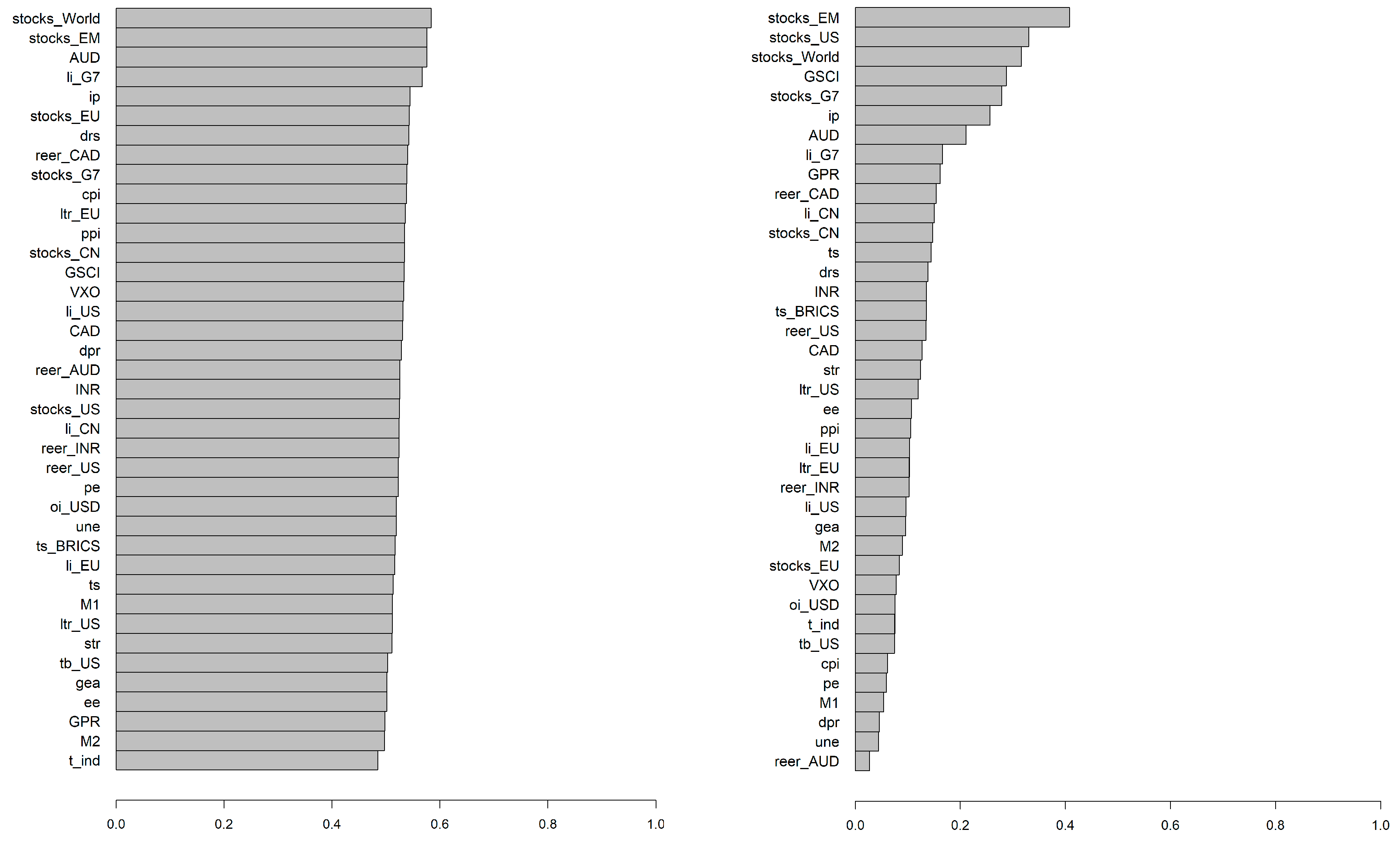
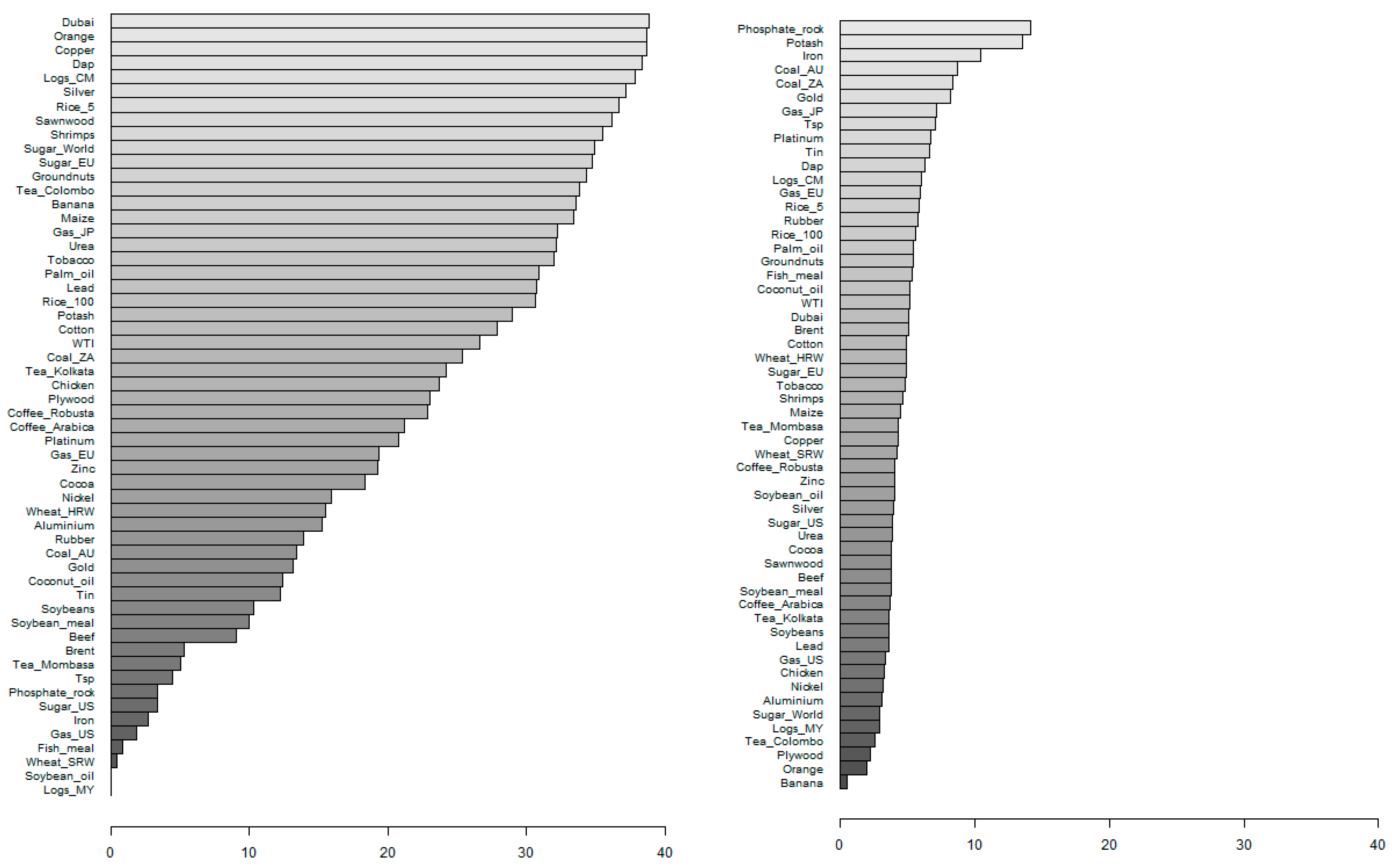
5.6. Overall Importance of Price Predictors

The analysed commodities were divided into four groups: energy, food, materials, and metals (i.e., Brent–Gas_JP, Cocoa–Tobacco, Logs_CM–Potash, and Aluminium–Silver, shown row-wise in Table A1 in Appendix A). Figure 3, Figure 4, Figure 5 and Figure 6 show the frequency of how often a given explanatory variable was important in predicting a commodity’s prices amongst these groups for the BSR av EW rec and DMA models. It can be seen that DMA was preferring more strongly certain variables, whereas BSR av EW rec was not strongly preferring any variable to such an extent. However, some conclusions can still be derived. In particular, for energy commodities, the GSCI seemed to be the most important price predictor. Interestingly, stocks_CN was also quite often chosen, more often than other stock market indices and some financial indicators such as str, dpr, ts, and dpr. In the case of food commodities, those most often chosen were stocks_EM and oi_USD. Furthermore, ts_BRICS was relatively more often chosen than, for example, some financial indicators and GPR. In the case of materials commodities, these were li_EU, stocks_G7, and stocks_US; dpr, gea, and str were rarely chosen. In the case of metals commodities, these were stocks_EM, stocks_US, and stocks_World; gea, t_ind and dpr were rarely chosen.
Next, the already considered variable importances were further analysed. In particular, it was computed how often a given explanatory variable was important (according to the previously introduced two criteria in Section 5.5) for a given commodity over the out-of-sample period. Next, it was computed whether this frequency was over 50% (over the out-of-sample period). Figure 7 reports the number of explanatory variables for each commodity for which this condition was met. It can be seen that in the case of the BSR av EW rec method, Dubai, Orange, Copper, Dap, Logs_CM, Silver, Rice_5, Sawnwood, and Shrimps prices were impacted by a relatively high number of explanatory variables. However, Brent, Tea_Mombasa, Tsp, Phosphate_rock, Sugar_US, Iron, Gas_US, Fish_meal, Wheat_SRW, Soybean_oil, and Logs_MY were impacted by relatively few explanatory variables. The BSR av EW rec method selected many more variables than the DMA method in general. In other words, the DMA method identified fewer variables as important price predictors. In particular, according to the DMA method, Phosphate_rock, Potash, and Iron were affected by the highest number of predictors, whereas Tea_Colombo, Plywood, Orange, and Banana were impacted by the smallest number of predictors.

6. Conclusions

In this study, a wide set of 56 commodities’ prices were analysed and 39 potentially important explanatory variables were used to capture various market, financial, and economic influences. In addition to Bayesian symbolic regression, other methods dealing with variable uncertainty were considered, as well as some standard simple benchmark models. The obtained forecasts were evaluated with various measures and tested with various methods. In many cases, the developed econometric methods were able to generate more accurate forecasts than simple benchmark models.
Although no strong evidence was found that Bayesian symbolic regression itself outperforms many of the other methods, it was also not found to be significantly less accurate. However, the way that Bayesian symbolic regression selects explanatory variables was not able to clearly detect certain patterns in the time-varying importance of predictors, contrary to other developed econometric methods such as Dynamic Model Averaging.
In the case of comparing “fixed” vs. recursive computations with symbolic regression (Bayesian, the standard one based on genetic programming, and the ones including model averaging schemes), surprisingly recursive computations only in certain cases resulted in more accurate forecasts than “fixed” estimations. However, in a reasonable number of cases the recursive version of Bayesian symbolic regression generated significantly more accurate forecasts than the standard symbolic regression based on genetic programming. In the case of Bayesian symbolic regression, the previous hypothesis, that a higher number of linear components should be chosen if forecast accuracy is the aim, was confirmed. However, the selection of an initial set of operators (functions) was found to be a less important issue. For example, the set of operators capturing non-linear effects was not selected often. This might be due to the symbolic regression algorithm itself evolving functions into sufficiently complicated forms.
According to the model confidence set, Dynamic Model Averaging was the most often selected amongst all of the models dealing with the variable uncertainty problem; however, symbolic regression was still selected in a reasonable number of cases. In particular, the Bayesian version was chosen rather than the standard one based on genetic programming. The recursive version of Bayesian symbolic regression outperformed benchmark models for certain commodities, especially around the 2008–2016 period.
More detailed analysis showed that the set of important commodity price predictors differed amongst different groups of commodities (i.e., energy, food, materials, and metals). In particular, this evidence could be derived from the Dynamic Model Averaging analysis. Finally, there was a clear difference between the number of important explanatory variables indicated for each commodity using Bayesian symbolic regression and Dynamic Model Averaging. In particular, Dynamic Model Averaging was more restrictive in this manner.
This study confirmed that outperforming standard benchmark models, such as ARIMA, is still a challenging task when forecasting commodities’ prices. It also confirmed the outcomes of some previous studies that Dynamic Model Averaging is a promising and high-performing method, outperforming, for example, LASSO, LARs, and RIDGE regressions. Nevertheless, Bayesian symbolic regression happened to also be an interesting and competing method with the standard symbolic regression based on genetic programming, and seems to be worth further studies and applications in economics and finance.

Author Contributions

Conceptualisation, K.D.; methodology, K.D.; software, K.D.; validation, K.D.; formal analysis, K.D.; investigation, K.D.; resources, K.D.; data curation, K.D.; writing—original draft preparation, K.D. and M.P.; writing—review and editing, K.D.; visualisation, K.D.; supervision, K.D.; project administration, K.D.; funding acquisition, K.D. All authors have read and agreed to the published version of the manuscript.

Funding

Research funded by the grant of the National Science Centre, Poland, under the contract number DEC-2018/31/B/HS4/02021.

Data Availability Statement

The data presented in this study are available in repositories explicitly cited in the paper.

Acknowledgments

Research funded by the grant of the National Science Centre, Poland, under the contract number DEC-2018/31/B/HS4/02021.

Conflicts of Interest

The authors declare no conflicts of interest. The funders had no role in the design of the study; in the collection, analyses, or interpretation of data; in the writing of the manuscript; or in the decision to publish the results.

Appendix A

Table A1. The list of analysed commodities.
AbbreviationDescription
BrentBrent oil
DubaiDubai oil
WTIWTI oil
Coal_AUCoal (Australia)
Coal_ZACoal (South Africa)
Gas_USGas (U.S.)
Gas_EUGas (Europe)
Gas_JPGas (Japan)
CocoaCocoa
Coffee_ArabicaCoffee Arabic
Coffee_RobustaCoffee Robusta
Tea_ColomboTea (Colombo)
Tea_KolkataTea (Kolkata)
Tea_MombasaTea (Mombasa)
Coconut_oilCoconut oil
GroundnutsGroundnuts
Fish_mealFish meal
Palm_oilPalm oil
SoybeansSoybeans
Soybean_oilSoybean oil
Soybean_mealSoybean meal
MaizeMaize
Rice_5Rice 5% broken
Rice_100Rice 100% broken
Wheat_SRWU.S. soft red winter wheat
Wheat_HRWU.S. hard red winter wheat
BananaBanana
OrangeOrange
BeefBeef
ChickenChicken
ShrimpsShrimps
Sugar_EUSugar (Europe)
Sugar_USSugar (U.S.)
Sugar_WorldSugar (world)
TobaccoTobacco
Logs_CMLogs (Cameroon)
Logs_MYLogs (Malaysia)
SawnwoodSawnwood
PlywoodPlywood
CottonCotton
RubberRubber
Phosphate_rockPhosphate rock
DapDiammonium phosphate
TspTriple superphosphate
UreaUrea
PotashPotash
AluminiumAluminium
IronIron ore
CopperCopper
LeadLead
TinTin
NickelNickel
ZincZinc
GoldGold
PlatinumPlatinum
SilverSilver
Table A2. Descriptive statistics.
VariableMeanStandard DeviationMedianMinMaxSkewnessKurtosis
Brent47.4932.2137.729.80133.900.82−0.48
Dubai45.2431.6334.2610.05131.200.81−0.52
WTI46.0928.7037.7711.31133.900.77−0.48
Coal_AU58.1031.0247.7022.25180.001.100.68
Coal_ZA54.6729.4646.6221.25167.800.950.20
Gas_US3.552.142.841.1913.521.753.68
Gas_EU5.553.394.041.5815.930.91−0.23
Gas_JP7.264.265.452.7218.110.92−0.32
Cocoa1.920.701.690.863.530.48−0.90
Coffee_Arabica2.881.102.841.176.620.700.53
Coffee_Robusta1.650.611.680.504.030.350.36
Tea_Colombo2.350.861.961.184.270.40−1.29
Tea_Kolkata2.160.562.071.034.070.48−0.29
Tea_Mombasa1.960.531.831.123.390.67−0.68
Coconut_oil819.90397.80703.00284.002256.001.050.46
Groundnuts1192.00405.401055.00618.202528.001.371.65
Fish_meal921.00474.00680.20339.001926.000.37−1.46
Palm_oil618.10252.60576.60234.001377.000.800.08
Soybeans343.30119.70307.00183.00684.000.79−0.36
Soybean_oil707.50283.80626.00286.901575.000.940.24
Soybean_meal307.20117.70270.00144.20651.400.74−0.46
Maize148.8059.99124.4075.27333.101.270.91
Rice_5354.20126.90321.20163.80907.000.890.93
Rice_100288.20126.40232.00120.80762.700.68−0.43
Wheat_SRW178.6061.97162.3085.30419.600.920.45
Wheat_HRW192.5067.55172.70102.20439.701.030.35
Banana0.710.280.650.251.300.32−1.18
Orange0.670.230.640.231.430.60−0.26
Beef3.051.082.691.636.180.65−0.65
Chicken1.600.401.530.882.720.35−0.83
Shrimps12.092.1411.887.5019.250.640.43
Sugar_EU0.540.120.550.340.78−0.11−1.23
Sugar_US0.530.100.490.380.891.823.09
Sugar_World0.280.110.260.110.651.010.88
Tobacco3611.00812.303400.002340.005118.000.31−1.35
Logs_CM355.5075.08344.80220.50562.800.46−0.56
Logs_MY248.3064.21251.80133.30520.800.901.53
Sawnwood694.20144.20713.30374.10973.60−0.20−0.91
Plywood497.9093.48499.90310.60751.800.09−0.67
Cotton1.640.491.610.825.062.8214.46
Rubber1.630.981.400.496.261.663.36
Phosphate_rock75.9567.4944.0031.00450.003.0812.69
Dap284.20163.50214.80112.801076.001.874.93
Tsp258.60165.80198.50105.101132.002.367.90
Urea202.80118.20185.8062.75785.001.463.31
Potash204.80129.90151.2083.00682.501.461.61
Aluminium1796.00442.901731.001040.003578.000.820.34
Iron67.3248.4037.9024.30214.401.180.31
Copper4365.002472.003221.001377.0010,160.000.45−1.25
Lead1279.00780.00935.50375.703720.000.47−1.12
Tin12,030.007412.008144.003694.0035,020.000.71−0.64
Nickel12,830.007342.0011,170.003872.0052,180.001.865.14
Zinc1702.00762.701528.00747.604405.000.860.10
Gold772.80506.80433.90256.101969.000.66−1.06
Platinum844.10442.30809.80341.202052.000.69−0.58
Silver11.818.527.033.6542.701.150.68
dpr−1.440.29−1.50−2.03−0.760.34−0.64
pe25.586.7725.4113.3244.200.680.22
str2.852.462.38−0.018.900.41−1.00
ltr_US4.582.214.460.629.360.29−0.90
ltr_EU4.833.034.25−0.0911.140.39−0.78
ts1.731.091.71−0.493.780.03−1.06
drs3.081.323.160.246.10−0.03−1.14
cpi192.8042.58191.60116.20273.10−0.02−1.24
ppi157.2035.17150.20104.80233.400.18−1.55
ip87.4614.1392.3560.59104.20−0.76−0.90
ee16.324.5715.849.2926.100.21−1.12
M11091.001204.00713.50614.107230.004.3217.86
M23680.001334.003335.002305.007636.001.010.25
gea2.4759.50−4.90−162.40188.600.730.86
une5.881.675.503.5014.701.312.36
AUD0.760.120.760.491.100.430.38
CAD0.810.110.790.621.050.42−0.69
INR2.551.282.221.327.692.174.62
reer_AUD95.0512.4396.6471.32123.900.22−0.60
reer_CAD106.1012.08102.9085.69128.400.20−1.32
reer_INR90.6712.6888.8364.62128.400.32−0.08
reer_US97.587.5796.8983.93114.600.28−0.99
tb_US−44,570.0025,260.00−48,220.00−97,680.00−3492.000.10−1.35
GSCI3525.001646.002990.001086.0010,560.001.131.20
oi_USD296,900,000,000.00275,400,000,000.00131,700,000,000.0027,050,000,000.00901,500,000,000.000.45−1.43
t_ind1.110.041.101.041.240.950.99
VXO19.958.2118.167.8761.381.633.97
GPR98.4248.7288.5739.05512.504.5829.51
stocks_US1330.00859.801187.00258.904523.001.171.28
stocks_World1210.00566.101149.00423.103141.000.760.33
stocks_G71080.00515.101022.00384.302907.000.910.68
stocks_EU307.50116.20336.3096.69582.30−0.14−0.91
stocks_EM659.40343.40542.30109.701376.000.19−1.37
stocks_CN44,140.0027,480.0040,970.002274.00141,100.000.37−0.26
ts_BRICS0.000.010.00−0.040.05−0.683.74
li_US99.771.3399.9192.31102.20−1.594.55
li_G799.861.22100.1092.26102.10−1.836.66
li_EU100.001.68100.1090.44103.20−1.092.99
li_CN99.971.41100.1085.68103.10−2.8225.36
Table A3. Stationarity tests. (“>” indicates “greater than”, and “<” indicates “smaller than”.).
VariableADF Stat.ADF p-Val.PP Stat.PP p-Val.KPSS Stat.KPSS p-Val.
Brent−7.9953<0.01−253.6471<0.010.0446>0.10
Dubai−8.2440<0.01−230.5171<0.010.0436>0.10
WTI−8.0483<0.01−248.0916<0.010.0400>0.10
Coal_AU−6.5208<0.01−280.4958<0.010.0801>0.10
Coal_ZA−6.1623<0.01−266.5725<0.010.0538>0.10
Gas_US−8.7802<0.01−361.7846<0.010.0348>0.10
Gas_EU−6.4891<0.01−277.7274<0.010.0560>0.10
Gas_JP−6.7223<0.01−229.5060<0.010.0636>0.10
Cocoa−7.3658<0.01−321.8202<0.010.0906>0.10
Coffee_Arabica−6.9581<0.01−314.2563<0.010.0674>0.10
Coffee_Robusta−6.2083<0.01−298.5168<0.010.1047>0.10
Tea_Colombo−8.1779<0.01−348.0611<0.010.0361>0.10
Tea_Kolkata−12.9817<0.01−282.5993<0.010.0150>0.10
Tea_Mombasa−7.1632<0.01−313.6262<0.010.0259>0.10
Coconut_oil−6.1340<0.01−323.9682<0.010.0421>0.10
Groundnuts−7.0198<0.01−284.0919<0.010.0233>0.10
Fish_meal−7.7946<0.01−275.7443<0.010.0601>0.10
Palm_oil−7.1712<0.01−269.1340<0.010.0642>0.10
Soybeans−7.6204<0.01−331.3422<0.010.0596>0.10
Soybean_oil−6.7782<0.01−263.4829<0.010.0627>0.10
Soybean_meal−8.0436<0.01−267.6929<0.010.0425>0.10
Maize−7.6244<0.01−299.4328<0.010.0389>0.10
Rice_5−8.7629<0.01−233.7177<0.010.0488>0.10
Rice_100−7.7580<0.01−231.1146<0.010.0521>0.10
Wheat_SRW−8.4273<0.01−309.6046<0.010.0353>0.10
Wheat_HRW−7.7958<0.01−304.6156<0.010.0413>0.10
Banana−11.8927<0.01−388.1070<0.010.0161>0.10
Orange−11.8850<0.01−268.7407<0.010.0232>0.10
Beef−7.7189<0.01−228.0717<0.010.1321>0.10
Chicken−10.5157<0.01−260.6561<0.010.0269>0.10
Shrimps−7.3627<0.01−196.4938<0.010.0356>0.10
Sugar_EU−7.4501<0.01−315.1929<0.010.1137>0.10
Sugar_US−6.3475<0.01−282.7717<0.010.0680>0.10
Sugar_World−7.3141<0.01−288.5904<0.010.0413>0.10
Tobacco−5.0524<0.01−287.2056<0.010.1256>0.10
Logs_CM−7.8160<0.01−292.3322<0.010.0386>0.10
Logs_MY−7.6421<0.01−255.3297<0.010.0395>0.10
Sawnwood−6.2682<0.01−333.6141<0.010.0931>0.10
Plywood−7.3099<0.01−281.7184<0.010.0430>0.10
Cotton−7.9502<0.01−194.0813<0.010.0387>0.10
Rubber−6.4845<0.01−295.2020<0.010.0616>0.10
Phosphate_rock−5.7667<0.01−381.9933<0.010.0363>0.10
Dap−6.9540<0.01−203.3954<0.010.0559>0.10
Tsp−7.3063<0.01−183.7721<0.010.0515>0.10
Urea−8.1881<0.01−302.8459<0.010.0324>0.10
Potash−6.2091<0.01−443.6662<0.010.1158>0.10
Aluminium−7.3307<0.01−337.5590<0.010.0697>0.10
Iron−6.3234<0.01−271.0289<0.010.0596>0.10
Copper−8.1452<0.01−233.0640<0.010.0946>0.10
Lead−6.5456<0.01−310.2747<0.010.0784>0.10
Tin−6.8723<0.01−298.2957<0.010.1397>0.10
Nickel−6.4269<0.01−249.7583<0.010.0438>0.10
Zinc−6.3570<0.01−293.2702<0.010.0385>0.10
Gold−6.6906<0.01−331.2990<0.010.51260.0388
Platinum−8.3714<0.01−306.8139<0.010.0952>0.10
Silver−7.5172<0.01−299.9199<0.010.1486>0.10
dpr−2.18080.5009−6.76320.73181.8097<0.01
pe−1.87320.6309−5.29900.81370.9871<0.01
str−3.50420.0423−9.12290.59994.6993<0.01
ltr_US−4.0658<0.01−31.5982<0.016.2708<0.01
ltr_EU−3.14250.0979−13.46120.35726.0577<0.01
ts−3.29580.0718−14.86520.27870.2490>0.10
drs−3.19720.0886−11.42790.47100.2997>0.10
cpi−6.6089<0.01−204.7199<0.010.8030<0.01
ppi−6.3383<0.01−249.5577<0.010.0516>0.10
ip−6.5356<0.01−298.2689<0.010.2861>0.10
ee−4.9675<0.01−393.8539<0.010.2569>0.10
M1−6.9325<0.01−365.9665<0.010.53290.0343
M2−6.0468<0.01−156.3054<0.011.3597<0.01
gea−2.44240.3905−22.57390.04110.67360.0159
une−2.54960.3451−21.16000.05390.39890.0776
AUD−7.0716<0.01−393.6667<0.010.0588>0.10
CAD−7.0035<0.01−413.4559<0.010.0908>0.10
INR−6.4130<0.01−364.1453<0.010.45520.0534
reer_AUD−7.9739<0.01−275.5769<0.010.0580>0.10
reer_CAD−7.3475<0.01−307.1186<0.010.0951>0.10
reer_INR−7.3033<0.01−325.3636<0.010.52380.0363
reer_US−7.6200<0.01−227.4906<0.010.0742>0.10
tb_US−5.7462<0.01−103.8847<0.010.1607>0.10
GSCI−7.0261<0.01−316.9545<0.010.2585>0.10
oi_USD−6.8621<0.01−330.9185<0.010.0850>0.10
t_ind−3.21370.0858−36.2523<0.013.5126<0.01
VXO−3.55020.0379−64.6624<0.010.2472>0.10
GPR−4.7256<0.01−103.1218<0.010.1747>0.10
stocks_US−6.1733<0.01−394.0153<0.010.1278>0.10
stocks_World−6.4726<0.01−374.9809<0.010.0608>0.10
stocks_G7−6.4349<0.01−377.8616<0.010.0720>0.10
stocks_EU−6.7591<0.01−375.6705<0.010.0936>0.10
stocks_EM−7.2645<0.01−344.3724<0.010.1365>0.10
stocks_CN−6.5398<0.01−415.8805<0.010.1967>0.10
ts_BRICS−4.9694<0.01−130.1868<0.010.39090.0811
li_US−4.9081<0.01−29.9440<0.010.0800>0.10
li_G7−5.2672<0.01−30.2912<0.010.0946>0.10
li_EU−5.4067<0.01−25.42110.02210.1003>0.10
li_CN−4.1257<0.01−82.3776<0.010.1147>0.10
Table A4. The Diebold–Mariano test—“best” model vs. ARIMA and vs. NAIVE.
CommodityBestBest vs. ARIMABest vs. NAIVE
BrentDMA0.00040.0002
DubaiDMA0.00010.0000
WTIBMA0.00040.0004
Coal_AUB-RIDGRE0.07290.0246
Coal_ZABSR av EW rec0.19060.0006
Gas_USDMA0.05390.2162
Gas_EUDMA0.44690.0114
Gas_JPDMA0.41780.0538
CocoaARIMA 0.1483
Coffee_ArabicaDMA0.46570.4603
Coffee_RobustaARIMA 0.1928
Tea_ColomboBMA0.32370.3149
Tea_KolkataBMA0.39720.1314
Tea_MombasaBMA0.26290.3450
Coconut_oilBMA0.15350.0087
GroundnutsDMA0.25850.0245
Fish_mealB-RIDGRE0.25760.4941
Palm_oilARIMA 0.0091
SoybeansBMA0.12580.0784
Soybean_oilDMA0.41970.0387
Soybean_mealARIMA 0.0007
MaizeBSR av EW rec0.29560.0795
Rice_5ARIMA 0.4718
Rice_100NAIVE0.4002
Wheat_SRWARIMA 0.3001
Wheat_HRWBMA0.45650.2907
BananaDMA0.42660.4133
OrangeARIMA 0.3381
BeefARIMA 0.1138
ChickenARIMA 0.2135
ShrimpsARIMA 0.0618
Sugar_EURIDGE0.08840.3505
Sugar_USARIMA 0.1307
Sugar_WorldARIMA 0.0090
TobaccoARIMA 0.2881
Logs_CMBMA0.11380.0181
Logs_MYARIMA 0.0251
SawnwoodDMA0.01500.0824
PlywoodDMA0.31200.2524
CottonARIMA 0.0036
RubberBMA0.40720.2832
Phosphate_rockGP fix0.04720.1994
DapARIMA 0.1316
TspARIMA 0.0446
UreaBSR av MSE rec0.14350.0868
PotashBMA0.12530.4778
AluminiumDMA0.00200.0010
IronRIDGE0.12580.0386
CopperDMA0.14590.0725
LeadARIMA 0.2022
TinDMA0.16510.1013
NickelARIMA 0.0693
ZincBMS 1V0.43680.0314
GoldBMA0.10370.1845
PlatinumBMA0.00130.0034
SilverDMS 1V0.24380.1263
Table A5. The Diebold–Mariano test—BSR rec model vs. “best”, vs. ARIMA, and vs. NAIVE.
CommodityBSR Rec vs. BestBSR Rec vs. ARIMABSR Rec vs. NAIVE
Brent0.00000.00240.0352
Dubai0.00000.52410.9577
WTI0.00850.05610.0825
Coal_AU0.01670.46240.1947
Coal_ZA0.01110.00170.1732
Gas_US0.11490.57880.1229
Gas_EU0.01510.02100.2298
Gas_JP0.03500.06960.2353
Cocoa0.00100.00100.0022
Coffee_Arabica0.00030.00020.0000
Coffee_Robusta0.15780.15780.1578
Tea_Colombo0.01180.01060.0085
Tea_Kolkata0.10530.03680.2181
Tea_Mombasa0.11840.12870.1229
Coconut_oil0.05570.07470.0877
Groundnuts0.00410.00010.0091
Fish_meal0.15840.15840.1584
Palm_oil0.09680.09680.1069
Soybeans0.04420.05160.0543
Soybean_oil0.06050.02250.8987
Soybean_meal0.00000.00000.0000
Maize0.05670.12680.1653
Rice_50.11740.11740.0821
Rice_1000.00080.16780.0008
Wheat_SRW0.11480.11480.0806
Wheat_HRW0.03600.05860.0628
Banana0.00160.16210.0015
Orange0.14210.14210.1424
Beef0.05940.05940.1950
Chicken0.03100.03100.0527
Shrimps0.01170.01170.0087
Sugar_EU0.05900.34080.0340
Sugar_US0.11200.11200.3439
Sugar_World0.15910.15910.1591
Tobacco0.11310.11310.1203
Logs_CM0.00060.02320.0948
Logs_MY0.00000.00000.0001
Sawnwood0.00020.04320.0610
Plywood0.00560.00690.0070
Cotton0.00050.00050.0164
Rubber0.00030.01820.0360
Phosphate_rock0.01550.92500.0061
Dap0.14080.14080.3374
Tsp0.11420.11420.8300
Urea0.04740.08680.2359
Potash0.08750.59450.1037
Aluminium0.00000.00300.0073
Iron0.22400.71910.9356
Copper0.01580.42150.6329
Lead0.02060.02060.1275
Tin0.15090.60050.8598
Nickel0.10160.10160.4385
Zinc0.40960.51210.8845
Gold0.16340.68380.6001
Platinum0.03190.06790.0675
Silver0.09820.34000.3480
Table A6. The Diebold–Mariano test—GP rec model vs. “best”, vs. ARIMA, and vs. NAIVE.
CommodityGP Rec vs. BestGP Rec vs. ARIMAGP Rec vs. NAIVE
Brent0.00000.00010.0038
Dubai0.00000.00010.0005
WTI0.00000.00920.0405
Coal_AU0.13050.78230.9500
Coal_ZA0.01070.27150.7661
Gas_US0.14990.15470.1528
Gas_EU0.00070.00180.0083
Gas_JP0.03630.05990.2664
Cocoa0.00000.00000.0000
Coffee_Arabica0.00040.00040.0005
Coffee_Robusta0.03010.03010.0301
Tea_Colombo0.00000.00000.0000
Tea_Kolkata0.00010.00000.0000
Tea_Mombasa0.00000.00000.0000
Coconut_oil0.00000.00000.0001
Groundnuts0.00000.00000.0000
Fish_meal0.15900.15900.1590
Palm_oil0.00090.00090.0209
Soybeans0.01250.01250.0125
Soybean_oil0.00110.00120.0514
Soybean_meal0.00000.00000.0002
Maize0.00040.00050.0005
Rice_50.10260.10260.1026
Rice_1000.00110.20120.0011
Wheat_SRW0.00000.00000.0000
Wheat_HRW0.03000.04480.0586
Banana0.00000.00000.0000
Orange0.12690.12690.1279
Beef0.03270.03270.0381
Chicken0.07620.07620.0588
Shrimps0.00000.00000.0000
Sugar_EU0.00120.00140.0001
Sugar_US0.07460.07460.1168
Sugar_World0.00000.00000.0000
Tobacco0.00000.00000.0000
Logs_CM0.00000.00030.0019
Logs_MY0.00000.00000.0000
Sawnwood0.00280.00290.0029
Plywood0.00000.00000.0000
Cotton0.00030.00030.0007
Rubber0.00620.04930.0585
Phosphate_rock0.26540.95340.4070
Dap0.04340.04340.0293
Tsp0.02090.02090.4023
Urea0.00000.00020.0005
Potash0.01870.47910.0157
Aluminium0.00000.00000.0001
Iron0.14230.48580.7309
Copper0.00040.05960.0722
Lead0.00810.00810.0111
Tin0.05660.18230.3743
Nickel0.00220.00220.0062
Zinc0.00010.00970.0310
Gold0.14490.47440.3852
Platinum0.01610.87650.8434
Silver0.45220.61010.6420
Table A7. The Diebold–Mariano test—“rec” vs. “fix”.
CommodityBSRBSR av MSEBSR av EWGP
Brent0.99970.00000.79990.9982
Dubai1.00000.00000.00440.9995
WTI0.15910.84090.00080.0005
Coal_AU0.31200.87510.00000.0000
Coal_ZA0.98300.04170.00030.6665
Gas_US0.19630.15550.00130.1225
Gas_EU0.12980.86610.14050.0000
Gas_JP0.15910.84090.04160.0314
Cocoa0.99300.00000.01240.0000
Coffee_Arabica0.99990.00040.00100.9980
Coffee_Robusta0.15910.84090.00000.9686
Tea_Colombo0.79480.00000.00001.0000
Tea_Kolkata0.74710.00000.84681.0000
Tea_Mombasa0.88120.00000.00120.0000
Coconut_oil0.92140.00000.00030.9972
Groundnuts0.99600.00000.00290.0000
Fish_meal0.84160.15900.03010.8410
Palm_oil0.13250.87680.02270.0000
Soybeans0.15850.01250.83630.9875
Soybean_oil0.31320.03140.07120.0000
Soybean_meal1.00000.00010.00110.9940
Maize0.93490.00040.00050.0000
Rice_50.87930.10270.04490.1594
Rice_1000.99730.02690.09040.9792
Wheat_SRW0.91440.00000.01350.9999
Wheat_HRW0.94000.06280.00000.0411
Banana0.86070.00000.20940.0001
Orange0.15910.84090.00000.1117
Beef0.89030.03370.06580.0000
Chicken0.97540.12100.68370.8680
Shrimps0.97390.00000.00160.0001
Sugar_EU0.97030.00020.16120.0083
Sugar_US0.66170.13120.53370.6361
Sugar_World0.84090.87270.04910.0379
Tobacco0.87060.00020.04030.9175
Logs_CM0.99900.00020.00400.0001
Logs_MY0.02270.97730.92121.0000
Sawnwood0.64730.00300.09060.0408
Plywood0.16480.80050.15910.7624
Cotton0.25960.78930.00040.0002
Rubber0.99740.02620.00000.9615
Phosphate_rock0.99650.31590.18990.7346
Dap0.07880.92120.00120.0044
Tsp0.52780.00600.07580.6297
Urea0.95260.00000.00851.0000
Potash0.89550.01810.11500.9811
Aluminium0.99990.00000.00000.9998
Iron0.51660.30030.03740.0418
Copper0.86250.00290.00000.1166
Lead0.95350.00130.00080.9830
Tin0.48070.10160.08060.0004
Nickel0.66660.00040.00240.0010
Zinc0.20260.00040.00550.1246
Gold0.38830.38780.01050.0000
Platinum0.96020.23260.00060.1839
Silver0.15610.84420.00000.0000
Table A8. The Diebold–Mariano test—BSR vs. GP.
CommodityBSR Rec vs. GP RecBSR Fix vs. GP Fix
Brent0.06550.8724
Dubai0.00021.0000
WTI0.72290.0188
Coal_AU0.94060.0000
Coal_ZA0.88990.9977
Gas_US0.15410.0816
Gas_EU0.33101.0000
Gas_JP0.68180.9523
Cocoa0.00090.0000
Coffee_Arabica0.25361.0000
Coffee_Robusta0.75450.9212
Tea_Colombo0.00000.9933
Tea_Kolkata0.00000.9952
Tea_Mombasa0.73400.0000
Coconut_oil0.36220.9736
Groundnuts0.00010.0000
Fish_meal0.50070.9910
Palm_oil0.87641.0000
Soybeans0.01250.9222
Soybean_oil0.02690.0000
Soybean_meal0.03471.0000
Maize0.00070.0000
Rice_50.10300.1589
Rice_1000.47540.9999
Wheat_SRW0.00000.8917
Wheat_HRW0.46740.7429
Banana0.00000.0000
Orange0.77250.1117
Beef0.29530.7829
Chicken0.53240.8318
Shrimps0.00000.0000
Sugar_EU0.00310.0063
Sugar_US0.32930.3542
Sugar_World0.84090.8409
Tobacco0.74581.0000
Logs_CM0.08010.0005
Logs_MY0.00010.0266
Sawnwood0.00300.0000
Plywood0.00010.6267
Cotton0.85320.0008
Rubber0.16521.0000
Phosphate_rock0.91170.7826
Dap0.45670.8416
Tsp0.05560.9980
Urea0.00061.0000
Potash0.31570.9868
Aluminium0.04361.0000
Iron0.30800.1071
Copper0.01580.1789
Lead0.09691.0000
Tin0.09720.0006
Nickel0.00270.0004
Zinc0.00080.2556
Gold0.31840.0001
Platinum0.95051.0000
Silver0.71290.0091

Appendix B

Below is a description of the time-varying importance of price predictors, based on the DMA model according to the procedure described in Section 5.5.
In particular, the dividend to price ratio had a mostly positive impact, especially for Coal_ZA, Phosphate_rock, and Dap up to 2000; Palm_oil, Cotton, Rubber, Phosphate_rock, Potash, and Tin around 2011–2015. This impact was negative for Coal_AU and Coal_ZA between 2010 and 2012; Phosphate_rock between 2003 and 2006; and Gold since 2018.
The price earnings ratio also had a mostly negative impact, especially on the following: Coal_ZA between 2001 and 2011; Coffee_Robusta between 2006 and 2020; Coconut_oil, Fish_meal, Palm_oil, Soybean_oil, Soybean_meal, and Maize around 2015–2018; Rice_5 and Rice_100 since 2020; Tobacco between 2099 and 2015; Potash and Iron between 2005 and 2009 and since 2017; Tin and Zinc between 2016 and 2018; and Gold since 2019. It was positive for Gas_EU between 2000 and 2003; Gas_JP since 2018; Phosphate_rock between 1999 and 2001 and since 2010; Potash between 2009 and 2014; and Tin between 2011 and 2015.
The short-term interest rate had a mostly negative impact, especially on Coal_Za before 2011 and Coal_AU between 2006 and 2011, and both of these commodities since 2019; Gas_JP and Groundnuts since 2019; Fish_meal before 2002; Rice_5 and Rice_100 between 2008 and 2010; Wheat_HRW between 1997 and 2001; Beef and Chicken between 2007 and 2009; Sugar_EU between 2009 and 2011; Rubber before 2011; Phosphate_rock between 2010 and 2015 and between 2018 and 2020; and Dap and Tsp between 2004 and 2011. It was also negative for various metals (i.e., Lead, Tin, Nickel, Zinc, Gold, Platinum and Silver) between 2000 and 2009 (but in different sub-periods for different metals). For Gold, this negative impact was also present between 2012 and 2015. There was a positive impact on Soybean_meal between 2014 and 2016; Tobacco before 2002; Rubber between 2012 and 2014; Phosphate_rock between 2004 and 2007 and between 2016 and 2018; and Iron between 1997 and 2001, between 2005 and 2009, and between 2014 and 2020.
The long-term interest rate for the U.S. had a mostly negative impact. For many commodities, this was especially seen around 2007–2011 (i.e., Dubai, WTI, Coconut_oil, Palm_oil, Soybean_oil, Maize, Whear_HRW, Beef, Sugar_US, Sugar_World, Tobacco, Rubber, Phosphate_rock, Dap, Tsp, Potash, Copper, Tin, Gold, Platinum, and Silver). Some negative impact was also present before 1999 for Fish_meal, Wheat_SRW, Wheat_HRW, Dap, Lead, and Silver. For Phosphate_rock, the negative impact was present between 2007 and 2020. A positive impact was present for Coal_AU between 1998 and 2000, Rubber between 2002 and 2003, Gas_JP between 2009 and 2010, Groundnuts since 2019, and Iron between 2006 and 2018.
On the other hand, the long-term interest rate for the Euro area had mixed impacts. It was negative for Brent and Dubai around 2011 and 2012, Coal_AU between 2003 and 2006 and between 2011 and 2019, Coffee_Robusta between 2001 and 2004 and between 2006 and 2009, Palm_oil between 2011 and 2013, Shrimps between 2016 and 2020, Sugar_World between 2016 and 2017, Tobacco before 2002 and between 2012 and 2015, Cotton between 2013 and 2014, Rubber between 2011 and 2014, Tsp since 2011, Iron since 2005, Copper between 2011 and 2013, Tin between 2009 and 2016, and Platinum between 2011 and 2016. A positive impact was present for Coal_ZA before 2001, Gas_EU between 1999 and 2004, Gas_JP between 2015 and 2016, Soybean_meal between 2015 and 2017, Logs_MY and Plywood before 1997, Phosphate_rock in several periods between 2008 and 2020, Tsp between 2007 and 2011, and Potash between 2009 and 2012 and between 2016 and 2020.
The term spread had a mixed impact. The impact was negative on all energy commodities in some periods around 2016 and 2020; Soybeans, Maize, Wheat_SRW and Wheat_HRW in some periods before 2002; Tea_Mombasa, Fish_meal, and Soybean_meal between 2009 and 2016; Tobacco between 2008 and 2012; Phosphate_rock since 2005; Potash between 2006 and 2009 and between 2015 and 2020. It was also negative for some metals (i.e., Iron, Copper, Lead, Tin, and Zinc) around 2015–2019. On the other hand, it was positive on Coffee_Arabica between 2014 and 2019, Coffee_Robusta between 1999 and 2005, Groundnuts since 2014, Fish_meal and Palm_oil between 1999 and 2003, Logs_CM between 2004 and 2007, Logs_MY between 2011 and 2016, Cotton and Rubber between 2002 and 2004, Iron between 2006 and 2014, and Gold after 2014.
The default return spread had a slightly more positive (than negative) impact on commodity prices. The positive impact was on WTI, Coal_AU, and Coal_ZA around 2019 and 2020; Coal_AU around 2008; Coal_ZA before 2002; Gas_EU since 2019; Gas_JP between 2011 and 2018; Coffee_Arabica and Coffee_Robusta between 1999 and 2002; Palm_oil between 2002 and 2004; Soybeans between 1997 and 2000; Soybean_oil between 2001 and 2006; wheat prices around 1999 and 2001; Sugar_World between 2002 and 2006; Logs_MY and Plywood between 1999 and 2001; Rubber between 2000 and 2002 and between 2012 and 2014; Phosphate_rock between 2006 and 2020; and Silver before 1997. The negative impact was on Tea_Mombasa between 2015 and 2018, Groundnuts since 2014, Fish_meal for several periods between 1999 and 2013, wheat prices since 2019, Tobacco before 2009, Logs_MY between 2012 and 2016, Dap and Tsp around 2007 and 2012, Iron between 2005 and 2017, Copper and Lead between 2015 and 2018, Zinc for several periods between 2006 and 2018, and Gold since 2013.
The U.S. Consumer Price Index for all urban consumers had a mostly negative impact. In particular, this was on most crude oil prices in various periods between 2000 and 2009 and since 2016; Coal_AU before 2002 and since 2016; Cocoa between 2002 and 2005 and between 2010 and 2020; Tea_Kolkata between 2008 and 2020; Coconut_oil since 2012; Fish_meal between 2000 and 2009; Soybean_meal between 2013 and 2016; Maize between 2009 and 2016; Shrimps between 2011 and 2016; Phosphate_rock before 1999; Tsp between 2012 and 2020; Potash between 2005 and 2020; Aluminium, Iron, Tin and Zinc around 2006–2009; Platinum between 1997 and 1999 and between 2011 and 2016. It had a positive impact on Gas_JP between 1999 and 2004, Palm_oil and Soybean_oil around 2001–2003, rice prices around 2010–2012, Wheat_HRW between 1997 and 2003, Tobacco between 2015 and 2020, Phosphate_rock between 2010 and 2018, Dap between 2009 and 2012, and Urea since 2014.
The U.S. Producer Price Index had a mostly negative impact. In particular, this was on oil prices, coal prices and Gas_US around 2004–2010; Cocoa between 2002 and 2007; Tea_Mombasa between 1997 and 2000; Coconut_oil between 2004 and 2006 and between 2010 and 2012; Palm_oil, Soybeans, Soybean_oil, Soybean_meal, and Maize in several periods between 2001 and 2019; wheat prices before 2016; Phosphate_rock between 2009 and 2018; Potash since 2005; Iron between 2005 and 2011; Zinc between 2011 and 2016; Gold between 2003 and 2014; and Platinum and Silver around 2008–2012. It had a positive impact on coffee prices since 2015, Tea_Kolkata since 2008, rice prices since 2020, Beef since 2015, Chicken before 2000, Shrimps between 2011 and 2015, Sugar_EU and Sugar_World since 2020, Tobacco between 2012 and 2017, Plywood between 2015 and 2020, Cotton since 2018, Dap since 2016, Tsp since 2007, and Urea between 2008 and 2014.
U.S. industrial production had a mostly positive impact, especially since 2008 on Coffee_Robusta, Soybeans, Sugar_EU, Potash, Aluminium, Iron, Tin, Nickel, and Zinc. Furthermore, it had a positive impact in shorter periods on Brent between 2003 and 2005, WTI between 2001 and 2006, all oil prices around 2008–2009, Gas_EU and Gas_JP between 2015 and 2020, Fish_meal between 2013 and 2020, Beef between 2015 and 2019, Sugar_US between 2011 and 2017, Tobacco between 2006 and 2009, Plywood between 2011 and 2016, Rubber between 2008 and 2017, Phosphate_rock before 2005, Platinum between 2016 and 2020, and Silver since 2020. It had a negative impact on Gas_EU and Soybeans around 2008, Orange and Sugar_US between 2000 and 2008, Logs_MY between 2012 and 2016, Phosphate_rock between 2012 and 2019, Gold between 2000 and 2008, and Platinum between 2000 and 2002.
U.S. average hourly earnings of production and nonsupervisory employees had a mixed impact on less commodities than the previously reported variables. In particular, it had a negative impact on oil prices before 2015, Tea_Mombasa between 2015 and 2019, Fish_meal between 2011 and 2014, Soybean_meal between 2004 and 2013, Tsp between 2002 and 2007, and Potash and Iron between 2005 and 2020. It had a positive impact on Gas_JP between 2004 and 2014; coffee prices between 2014 and 2020; Sugar_EU between 2009 and 2013; Cotton between 2010 and 2017; Phosphate_rock before 2003 and since 2009; and Aluminium, Copper, Zinc, Gold and Platinum around 2006–2009.
The M1 money stock for the U.S. and M2 money stock for the U.S. had sometimes contradictory impacts, whereas M2 seemed to have more impact overall than M1. In particular, M1 had a negative impact on Cocoa between 2004 and 2007 and between 2018 and 2020, Palm_oil between 2001 and 2004, Orange between 2001 and 2008, Sugar_EU between 2008 and 2012, Sugar_World between 2001 and 2005, logs prices before 1998, Sawnwood and Plywood around 2009–2011, Phosphate_rock between 2008 and 2020, Dap between 2009 and 2012, Potash between 2005 and 2017, and Iron between 2015 and 2018. M1 had a positive impact on coal prices around 2001–2008, Gas_EU and Gas_JP around 2018–2020, Maize before 2002, Tsp and Urea around 2012–2015, Iron between 2009 and 2013, and Silver between 2001 and 2008. M2 had a negative impact on coal prices and gas prices around 2015–2019; Tea_Kolkata between 2015 and 2020; Coconut_oil between 2011 and 2017; Palm_oil, Soybeans, and Soybean_oil around 2003–2012; Sugar_EU before 2002; Sugar_US between 2008 and 2020; logs prices around 2000; Cotton before 2008 and between 2014 and 2020; Rubber and Phosphate_rock before 1999; Dap and Tsp between 2007 and 2017; and Lead between 2008 and 2018. M2 had a positive impact on Groundnuts and Fish_meal since 2013, rice prices between 2010 and 2013, wheat prices between 2001 and 2004, Chicken and Tobacco between 2014 and 2019, Phosphate_rock since 2008, Potash between 2009 and 2017, Gold and Platinum between 2014 and 2020, and Silver between 2018 and 2020.
Killian’s Index of Global Real Economic Activity had a mostly positive impact. In particular, this was on coal prices for almost all of the analysed period; Gas_EU and Gas_JP around 2008–2011 and since 2015; Tea_Mombasa and Coconut_oil since 2020; Soybeans, Soybean_meal, Maize, rice prices, and wheat prices before 2003; Soybeans, Soybean_oil, and Soybean_meal around 2008; Sugar_US between 2011 and 2018; Sugar_World between 2000 and 2003; Tobacco between 2014 and 2018; Sawnwood since 2019; Phosphate_rock since 2009; Dap since 2011; Potash since 2016; Iron since 2004; Lead and Zinc around 2004; and Silver between 1998 and 1999. However, it was negative on Dubai and WTI between 2001 and 2004, Palm_oil and rice prices around 2008–2011, Beef before 1998, Chicken between 2015 and 2020, Potash between 2009 and 2013, and Platinum between 2008 and 2011.
The U.S. unemployment rate had a rather negative impact, in particular on oil prices and Gas_EU around 2000, Coal_ZA before 2010, Groundnuts since 2020, Fish_meal between 1997 and 1998, rice prices around 2008 and since 2020, Sugar_US between 2009 and 2015, Phosphate_rock between 2000 and 2003 and between 2006 and 2017, Dap before 2000, Tsp and Urea before 1997, Potash since 2006, and Iron between 2004 and 2009. However, it had a positive impact on Gas_EU and Gas_JP around 2010; Coffee_Robusta between 2005 and 2006; Wheat_HRW between 1997 and 2003; Sugar_World between 2002 and 2005; Tobacco before 2002; and Iron, Copper, Lead, Tin, Nickle, and Platinum around 2009.
U.S. dollar exchange rates had a mostly positive impact. Mostly, this was indicated by the Australian dollar to U.S. dollar exchange rate, and, secondly, by the Indian rupee to U.S. dollar exchange rate. The impact from the Canadian dollar to U.S. dollar exchange rate was least often observed.
In particular, the Australian dollar to U.S. dollar exchange rate had a positive impact on Coal_AU between 1997 and 2002, between 2008 and 2011, and since 2017; Coal_ZA between 2001 and 2005 and between 2008 and 2015; Gas_EU in similar periods as for Coal_ZA, Cocoa, and coffee prices around 2009; Tea_Mombasa between 2006 and 2013; Groundnuts between 2011 and 2019; Palm_oil between 2007 and 2013; Soybeans and Soybean_meal between 2004 and 2016; Soybean_oil between 2009 and 2012 and between 2015 and 2017; Rice_100 and wheat prices between 2012 and 2016; wheat prices since 2019; Beef since 2016; Logs_CM since 2003; Sawnwood between 1998 and 2004; Plywood between 2005 and 2008; Cotton between 2007 and 2011; Rubber between 1998 and 2012; Tsp since 2008; and various metal prices around 2005, 2009, and 2020. In the case of metals, those mostly impacted were Aluminium, Copper, Lead, Nickel, Platinum, and Silver. However, the impact was negative on oil prices since 2016, Phosphate_rock between 2008 and 2016 and since 2020, and Potash between 2009 and 2016.
The Canadian dollar to U.S. dollar exchange rate had a positive impact on Gas_EU between 2008 and 2016; Gas_JP between 1998 and 2009; Cocoa between 2012 and 2016; Tea_Kolkata between 2001 and 2008; Coconut_oil, Soybeans, Wheat_HRW, Phosphate_rock, Tsp, and Gold around 2009; Tobacco between 2012 and 2013; Iron, Gold, Platinum, and Silver since 2016; and Gold in several periods since 2000. It had a negative impact on oil prices around 2004–2007 and 2015; Coal_AU between 2008 and 2010 and around 2015; Gas_US between 1998 and 2001 and around 2003, 2009, and 2017; Coffee_Arabica between 2006 and 2009; Sawnwood between 1998 and 2008; and Phosphate_rock in several periods before 2006.
The Indian rupee to U.S. dollar exchange rate had a positive impact on Coal_ZA since 2011, Coffee_Robusta between 2009 and 2020, Maize in several periods since 2006, Rubber between 2008 and 2019, Urea before 2004, Potash between 2008 and 2015, Iron between 2005 and 2019, Platinum in several periods between 1997 and 2019, and Silver around 2009 and between 2011 and 2014. It also had a positive impact on several other commodities (i.e., Dubai, Coffee_Arabica, Tea_Kolkata, Tea_Mombasa, Coconut_oil, Fish_meal, Palm_oil, Soybean_oil, Soybean_meal, and wheat prices) around 2009. It had a negative impact on Coal_AU and Gas_US before 1998, Gas_US between 2004 and 2007, Groundnuts since 2014, Phosphate_rock since 2008, and Potash since 2016.
In the case of real effective exchange rates, the one based on the manufacturing Consumer Price Index for Australia and the one based on the manufacturing Consumer Price Index for India had mostly positive impacts, whereas the one based on the manufacturing Consumer Price Index for Canada and the one based on the manufacturing Consumer Price Index for the U.S. had mostly negative impacts.
In particular, the real effective exchange rate based on the manufacturing Consumer Price Index for Australia had a positive impact on Brent, Dubai, coal prices, Palm_oil, Soybean_oil, Sugar_EU, Phosphate_rock, and Urea in various periods since 2011; Coffee_Robusta between 2005 and 2011; Beef between 2009 and 2015; Cotton between 2002 and 2013; Urea before 2005; Potash between 2007 and 2017; and Iron between 1999 and 2003. It had a negative impact on Gas_EU since 2008, Sugar_US between 2001 and 2014, and Phosphate_rock since 2010.
Real effective exchange rates based on the manufacturing Consumer Price Index for Canada had a negative impact on Coal_AU, Gas_US, Coffee_Arabica, Coconut_oil, Palm_oil, rice prices, Beef, and Tin in several periods after 2009; Coffee_Robusta between 1997 and 2016; Tea_Colombo before 2003; Soybeans, Soybean_meal, sugar prices, logs prices, Phosphate_rock, Tsp, and Copper around 2009–2013; Sawnwood before 1999; Platinum between 2008 and 2014; and Coffee_Arabica around 1997–2002. It had a positive impact on Gas_EU and Tea_Kolkata since 2017, Phosphate_rock between 2000 and 2004, and Potash since 2005.
Real effective exchange rates based on the manufacturing Consumer Price Index for India had a positive impact on Coal_AU in several sub-periods over the whole analysed time period, Tean_Mombasa between 2001 and 2020, Fish_meal between 2009 and 2020, rice prices around 2020, Wheat_HRW between 2003 and 2008, Chicken since 2013, Sawnwood between 1998 and 2005, Plywood since 2017, Tsp between 2012 and 2016, Iron between 2009 and 2013, and Tin around 2009. They had a negative impact on oil prices around 1999, coffee prices since 2018, Tea_Colombo since 2013, Tea_Kolkata between 2009 and 2013, Plywood between 2003 and 2008, Potash since 2005, Copper around 2007 and since 2016, Nickel since 2012, Zinc since 2019, and Silver between 2008 and 2009.
Real effective exchange rates based on the manufacturing Consumer Price Index for the U.S. had a positive impact on Gas_US and Gas_JP since 2020; Tea_Kolkata since 2013; Tea_Mombasa between 1998 and 2002; Orange in several sub-periods since 2008; Beef before 1998 and between 2005 and 2009; Shrimps and Sugar_EU around 2014–2018; Cotton before 2002; Copper, Tin, and Silver around 2007; and Copper Nickel and Silver since 2020. It had a negative impact on Coal_AU and Cola_ZA around 2015–2017, Cocoa since 2017, Tea_Mombasa between 2010 and 2015, Fish_meal, Palm_oil and Soybeans since 2019, Soybean_meal and rice prices since 2009, Shrimps before 2002, Sugar_EU between 2003 and 2012, Logs_CM over the whole analysed period, Sawnwood between 1999 and 2006 and since 2017, Rubber between 2013 and 2016, Phosphate_rock between 2003 and 2006, Urea between 2015 and 2018, Iron since 2005, and Lead and Zinc around 2005.
The U.S. trade balance had a mixed impact. It was positive mostly after 2006, in particular, on Coal_AU since 2005; Coal_ZA since 2018; Tea_Colombo since 2017; Iron between 2013 and 2019; and Coconut_oil, Soybeans, Soybean_oil, Soybean_meal, Maize, Rice_100, Sugar_EU, Sugar_US, Sugar_World, Phosphate_rock, Dap, and Tsp around 2008. It was negative on oil prices between 2000 and 2007, Gas_EU and Gas_JP between 2003 and 2011, Groundnuts between 2002 and 2007, Shrimps in several periods since 2003, Logs_CM between 2002 and 2006, Logs_MY and Plywood since 2015, Aluminium between 2000 and 2009, Iron between 2003 and 2009, and Copper around 2000.
The S&P GSCI Commodity Total Return Index had a positive impact on the majority of commodities and over multiple periods. In particular, this was on oil prices during the whole analysed period; Coal_AU since 2002; Coal_ZA since 2009; Gas_US, Tea_Mombasa, and Tin over almost whole analysed period; Gas_US since 2009; Gas_EU since 2017; Gas_JP before 2015; Tea_Kolkata before 2004; Soybean_meal between 1997 and 2005; Wheat_HRW between 1998 and 2003; Beef between 2008 and 2015; Rubber between 2008 and 2019; Dap between 2009 and 2014; Urea before 1999; Potash since 2005; Aluminium since 2009; Copper since 2007; Zinc between 2017 and 2019; Gold between 2001 and 2015; Platinum between 2013 and 2015; and Silver between 2011 and 2015. However, it had a negative impact on Groundnuts since 2014, Soybean_oil between 2003 and 2007, and Phosphate_rock since 2016.
The dollar open interest had a mostly positive impact, in particular, on Cocoa, coffee prices, Palm_oil, Soybean_meal, and Cotton in various periods after 2010; Coconut_oil in various sub-periods of the whole analysed period; Fish_meal between 1999 and 2006; Maize between 2005 and 2017; rice prices and Sugar_US between 2009 and 2018; Sugar_World between 2010 and 2020; Phosphate_rock between 1999 and 2001 and between 2009 and 2013; Dap between 2014 and 2017; and Platinum between 2006 and 2020. It had a negative impact on oil prices between 1997 and 2003 and around 2020; Gas_EU before 2004; Gas_JP since 2003; Tea_Kolkata between 2014 and 2019; Tea_Mombasa between 2006 and 2018; rice prices, Orange, and Chicken around 2001; and Potash between 2005 and 2010 and since 2014.
Working’s dollar T-index had a mostly negative impact, in particular, on oil prices around 2016; Coal_AU since 2005; Coal_ZA between 2001 and 2015; Gas_JP between 2002 and 2008 and since 2017; Coconut_oil, Groundnuts, Palm_oil, Soybean_oil, Maize, Wheat_HRW, and Sugar_EU around 2008–2014; Chicken and Shrimps since 2004; Rubber between 2012 and 2014; Phosphate_rock since 2013; Dap between 2009 and 2015; Tsp since 2010; Urea between 2012 and 2014; Tin between 2007 and 2015; and Platinum between 2008 and 2015. It had a positive impact on Coal_ZA and Dap before 1999, Gas_EU between 2010 and 2012, Coffee_Robusta between 2005 and 2007, Fish_meal before 2002, and Potash since 2005.
The VXO index of implied volatility had a mixed impact. It was negative on: oil prices around 2008 and 2020–2021, Coal_ZA and Gas_US before 1998, Coal_AU and Gas_US between 2018 and 2020, Chicken between 2001 and 2005, Rubber between 2008 and 2014, Dap since 2010, Urea between 2011 and 2015, Potash between 2005 and 2020, Lead between 1997 and 2001 and between 2008 and 2013, and Gold in various periods before 2014. It was positive on Coal_AU between 2005 and 2009; Gas_EU between 2010 and 2014; Coconut_oil between 2012 and 2019; Groundnuts since 2017; Palm_oil, Soybeans, Soybean_oil, Soybean_meal, Maize, and rice prices around 2020; wheat prices between 2015 and 2019; Cotton between 2012 and 2019; Phosphate_rock since 2009; and Tin around 2006–2007.
The Global Geopolitical Risk Index had a limited impact. It was negative on Dubai between 2004 and 2014; Coal_AU between 2004 and 2009; Coal_ZA before 2013; Soybeans, Soybean_oil, Soybean_meal, Maize, and Rice_5 since 2020; Tobacco since 2015; Rubber, Gold, and Silver since 2018; Phosphate_rock between 2009 and 2017; and Potash since 2006. It was positive on Rice_100 before 2002, Sawnwood between 1998 and 2001, Dap and Tsp since 2009, Aluminium and Lead since 2017, Iron between 2008 and 2017, and Tin between 2001 and 2017.
Stock prices had a mixed impact. The S&P 500 Index and the MSCI G7 index had mostly negative impacts, whereas the MSCI WORLD for developed markets index, the MSCI EU index, and the MSCI EM for emerging markets index had mostly positive impacts.
In particular, the S&P 500 Index had a negative impact on oil prices before 2001 and since 2015, coal prices between 2002 and 2005 and since 2017, Cocoa in various periods since 2003, Tea_Colombo between 2008 and 2016, Tea_Mombasa between 2015 and 2020, wheat prices around 2010–2015 and since 2019, Orange between 2009 and 2014, Sugar_EU over the whole analysed period, Sugar_World between 2013 and 2017, logs prices around 2006–2008, Logs_CM between 2010 and 2014, Logs_MY since 2014, Sawnwood since 2000, Urea between 2001 and 2008, Iron since 2008, Copper since 2016, Lead before 1999, Tin since 2014, Nickel between 2011 and 2016, Zinc since 2019, Gold and Platinum over the whole analysed period, and Silver since 2006. It was positive on rice prices around 2000–2001 and between 2008 and 2015, Phosphate_rock since 2009, Dap between 2009 and 2013, and Potash between 2009 and 2013.
In the case of the MSCI G7 index since 2015, the impact was positive (opposite than that of the S&P 500 Index) on oil prices. It was also positive on Groundnuts since 2013, Shrimps since 2011, Cotton between 2011 and 2019, Phosphate_rock between 2010 and 2016, Gold in various periods between 1997 and 2016, Platinum in various periods before 2008, and Silver between 1998 and 2002. It was negative on Coal_ZA between 2001 and 2010 and since 2017; Cocoa between 2001 and 2010; Tea_Colombo and Tea_Kolkata around 2010–2013; Fish_meal, Palm_oil and Soybeans around 1998–2001; rice prices in various sub-period of the whole analysed period; wheat prices since 2009; Logs_CM since 2002; Dap since 2009; Tsp before 2006; Potash since 2013; and Copper, Lead, Tin, Nickel, and Zinc between 2007 and 2016.
The MSCI WORLD for developed markets index had a positive impact on Brent since 2015; Coal_ZA and Gas_US around 2007–2010 and 2018; Cocoa between 2003 and 2014; Tea_Colombo and Tea_Mombasa around 2011–2015; Rice_5 before 2006 and both rice prices around 2012; wheat prices between 2013–2018; and Iron, Copper, Lead, Tin, Nickel, and Zinc around 2010. In the case of individual metals, the positive impact was observed in some other periods before or after 2010. In the cases of Gold and Platinum, it was positive over almost the whole analysed period. The MSCI WORLD for developed markets index had a negative impact on Tea_Mombasa and Groundnuts since 2014, Shrimps since 2010, Logs_CM in various period since 2003, Rubber between 2003 and 2006, Phosphate_rock since 2009, Dap between 2008 and 2016, Tsp in various periods since 2014, Potash between 2006 and 2014, and Silver between 1998 and 2002.
The MSCI EU index had a positive impact on oil prices around 2009; Tea_Mombasa and Coconut_oil between 2017 and 2020; Palm_oil before 2001; Rice_5 between 2004 and 2012; wheat prices since 2018; Sugar_EU in various sub-periods of the whole analysed period; Logs_CM since 2002; Logs_MY, Sawnwood, and Plywood between 2015 and 2018; and Tin between 2010 and 2017. It had a negative impact on Coal_ZA before 1997 and between 2001 and 2010, Gas_US since 2017, Rice_5 and Beef between 2014 and 2017, and Phosphate_rock and Dap around 2012–2014.
The MSCI EM for the emerging markets index had a positive impact on the majority of commodities, and it was mostly after 2015. In particular, this was on oil prices, coal prices, Coconut_oil, Groundnuts, Palm_oil, Soybeans, Soybean_oil, Shrimps, Sugar_US, Potash, and metals. In the case of Gold, Platinum, and Silver, the impact was present even since 2010. Maize, rice prices, wheat prices, Banana, and Orange were impacted positively around 2005–2015. The impact was negative on Gas_US between 2000 and 2010; Cocoa before 2001; Logs_CM and Phosphate_rock over almost the whole analysed period; Dap, Tsp, and Urea before 1998; Plywood before 1999; and Tsp since 2011.
The index representing the Chinese stock market had a slightly more negative than positive impact. It became an important price predictor in around 2008. In particular, it had a negative impact on oil prices around 2009 and since 2015; coal prices since 2017; Gas_EU and Gas_JP since 2010; Rice_5 between 2008 and 2014; both rice prices around 2009 and around 2011; Beef since 2015; Sawnwood since 2006; Gold since 2016; and Copper, Lead, and Tin around 2016. It had a positive impact on Tea_Mombasa since 2016, Fish_meal since 2013, Maize between 2005 and 2008, Chicken since 2016, Cotton and Rubber around 2020, Phosphate_rock between 2009 and 2015, Iron since 2009, Tin in various periods before 2008, and Nickel between 2009 and 2015.
The share of BRIC countries’ trade in the total global trade had a mixed impact. In particular, it was positive on Gas_EU between 2014 and 2017, coffee prices before 1999 and between 2010 and 2014, Fish_meal between 2008 and 2020, Rice_100 around 1997, between 2004 and 2007 and between 2014 and 2017, wheat prices between 2017 and 2020, Shrimps before 2007 and between 2010 and 2013, Logs_MY and Plywood between 2009 and 2011, Cotton between 2010 and 2015, Dap and Tsp before 1998, Potash between 2009 and 2018, and Copper before 1998 and between 2006 and 2009. It was negative on oil prices around 2018; coal prices since 2018; Coffee_Robusta, Tea_Colombo and Tea_Kolkata around 2019; Coconut_oil and Groundnuts since 2018; sugar prices around 2016–2017; Sugar_World before 2004; Tobacco between 2001 and 2016; Sawnwood before 2006; Phosphate_rock since 2009; Dap, Tsp, and Urea around 2010–2014; Iron between 2009 and 2013; Aluminium, Lead, Nickel, and Silver around 2019; Zinc between 2016 and 2019; Gold between 1996 and 2004, between 2011 and 2014, and since 2019; and Platinum between 1999 and 2001 and between 2009 and 2019.
In the case of leading indicators, those for the U.S. had a rather negative impact, whereas those for G7 countries, the Euro area, and China had a mostly positive impact. Similarly, as before, the variables linked with the Chinese market and the Euro area became important mostly after 2008.
In particular, the leading indicator for the U.S. had a negative impact on oil and coal prices since 2020, Gas_EU between 2010 and 2013, Gas_JP around 2010 and since 2016, Groundnuts between 2013 and 2017, Fish_meal before 2013, Palm_oil and Soybean_oil around 2006, Soybean_meal between 1997 and 200, Sugar_US between 2009 and 2020, Tobacco between 1998 and 2009, Phosphate_rock between 2001 and 2007, Potash between 2009 and 2013, Iron since 2001, Zinc and Platinum around 2008, and Gold between 2015 and 2019. It had a positive impact on coffee prices before 1997, logs prices before 1998, Plywood and Cotton around 1998; Phosphate_rock since 2009; Aluminium and Copper around 1997; Tin, Platinum and Silver around 2008; and, moreover, Platinum between 2000 and 2002.
The leading indicator for the G7 countries had a positive impact on oil prices around 2009, Coal_AU and Gas_JP in various sub-periods of the whole analysed period; Gas_EU between 2002 and 2004 and between 2010 and 2013; Coconut_oil between 2015 and 2019; Fish_meal between 1998 and 2009; wheat prices around 2016–2017; Tobacco between 1998 and 2009; Logs_CM between 2008 and 2018; Cotton between 2013 and 2018; Dap and Tsp around 2020; Ureal between 2016 and 2020; Iron between 2009 and 2017; Copper before 2009; Tin, Nickel and Zinc around 2008; and Platinum around 2000, between 2002 and 2004, and between 2008 and 2011. It had a negative impact on oil prices since 2020, Coconut_oil between 2001 and 2003, Groundnuts between 2013 and 2018, wheat prices around 1997, Logs_MY, Sawnwood and Plywood before 2000, Phosphate_rock since 2009, Potash since 2014, Gold since 2013, and Silver since 2020.
The leading indicator for the Euro area had a positive impact on oil prices around 2009 and since 2020, coal prices since 2008, Groundnuts since 2013, Palm_oil, Soybean_oil and Maize between 2008 and 2019, rice prices around 2008–2009, wheat prices before 1998 and between 2007 and 2014, logs prices between 2016 and 2020, Rubber between 1997 and 2005, Phosphate_rock, Dap, Tsp and Potash since 2008, and Gold since 2013. It had a negative impact on Gas_EU between 2010 and 2014, Gas_JP between 2001 and 2007, Coffee_Arabica between 1997 and 2000 and between 2002 and 2005, Tobacco between 1998 and 2009 and between 2016 and 2017, Iron between 2005 and 2008, Copper around 2008 and since 2020, and Zinc between 2006 and 2013.
The leading indicator for China had a positive impact on oil prices since 2020; coal prices between 2009 and 2011; rice prices between 2009 and 2017; wheat prices before 1999; Chicken between 2008 and 2016; Phosphate_rock between 2004 and 2008; Dap between 2008 and 2011 and between 2014 and 2020; Tsp between 2008 and 2020, Potash between 2011 and 2015; and Tea_Colombo, Palm_oil, Soybean_oil, Sugar_World, Sawnwood, Cotton, Copper, Tin, Zinc, Platinum, and Silver since 2020. It had a negative impact on oil prices around 2006, Gas_JP between 2001 and 2008, between 2011 and 2015 and since 2017, Logs_CM before 2002, Cotton and Rubber between 2013 and 2019, Phosphate_rock between 2009 and 2016, Iron between 2005 and 2013 and between 2017 and 2020, Copper around 2014–2018, Nickel and Zinc between 2008 and 2019, and Gold between 2006 and 2007.

References

  1. Abd Elaziz, Mohamed, Ahmed A. Ewees, and Zakaria Alameer. 2020. Improving adaptive neuro-fuzzy inference system based on a modified salp swarm algorithm using genetic algorithm to forecast crude oil price. Natural Resources Research 29: 2671–86. [Google Scholar] [CrossRef]
  2. Aguilar-Rivera, Rubén, Manuel Valenzuela-Rendon, and J. Rodriguez-Ortiz. 2015. Genetic algorithms and Darwinian approaches in financial applications: A survey. Expert Systems with Applications 42: 7684–97. [Google Scholar] [CrossRef]
  3. Ahumada, Hildegart, and Magdalena Cornejo. 2015. Explaining commodity prices by a cointegrated time series-cross section model. Empirical Economics 48: 1667–90. [Google Scholar] [CrossRef]
  4. Akram, Qaisar Farooq. 2009. Commodity prices, interest rates and the dollar. Energy Economics 31: 838–51. [Google Scholar] [CrossRef]
  5. Alam, Md Rafayet, and Scott Gilbert. 2017. Monetary policy shocks and the dynamics of agricultural commodity prices: Evidence from structural and factor-augmented VAR analyses. Agricultural Economics 48: 15–27. [Google Scholar] [CrossRef]
  6. Alameer, Zakaria, Ahmed Fathalla, Kenli Li, Haiwang Ye, and Jianhua Zhang. 2020. Multistep-ahead forecasting of coal prices using a hybrid deep learning model. Resources Policy 65: 101588. [Google Scholar] [CrossRef]
  7. Alameer, Zakaria, Mohamed Abd Elaziz, Ahmed A. Ewees, Haiwang Ye, and Jianhua Zhang. 2019a. Forecasting copper prices using hybrid adaptive neuro-fuzzy inference system and genetic algorithms. Natural Resources Research 28: 1385–401. [Google Scholar] [CrossRef]
  8. Alameer, Zakaria, Mohamed Abd Elaziz, Ahmed A. Ewees, Haiwang Ye, and Jianhua Zhang. 2019b. Forecasting gold price fluctuations using improved multilayer perceptron neural network and whale optimization algorithm. Resources Policy 61: 250–60. [Google Scholar] [CrossRef]
  9. Algieri, Bernardina, Matthias Kalkuhl, and Nicolas Koch. 2017. A tale of two tails: Explaining extreme events in financialized agricultural markets. Food Policy 69: 256–69. [Google Scholar] [CrossRef]
  10. Aloui, Riadh, Mohamed Safouane Ben Aissa, and Duc Khuong Nguyen. 2013a. Conditional dependence structure between oil prices and exchange rates: A copula-GARCH approach. Journal of International Money and Finance 32: 719–38. [Google Scholar] [CrossRef]
  11. Aloui, Riadh, Shawkat Hammoudeh, and Duc Khuong Nguyen. 2013b. A time-varying copula approach to oil and stock market dependence: The case of transition economies. Energy Economics 39: 208–21. [Google Scholar] [CrossRef]
  12. Al-Qudsi, Sulayman. 2010. Oil and commodity price volatility: Origins and impact on the Arab economy and capital markets. Geopolitics of Energy 32: 3–24. [Google Scholar]
  13. Alquist, Ron, Lutz Kilian, and Robert Vigfusson. 2013. Forecasting the price of oil. In Handbook of Economic Forecasting 2. Edited by Graham Elliott, C. Granger and Allan Timmermann. Amsterdam: Elsevier, pp. 427–507. [Google Scholar]
  14. Andreasson, Pierre, Stelios Bekiros, Duc Khuong Nguyen, and Gazi Salah Uddin. 2016. Impact of speculation and economic uncertainty on commodity markets. International Review of Financial Analysis 43: 115–27. [Google Scholar] [CrossRef]
  15. Apergis, Nicholas, and James E. Payne. 2010. Renewable energy consumption and economic growth: Evidence from a panel of OECD countries. Energy Policy 38: 656–60. [Google Scholar] [CrossRef]
  16. Arango, Luis, Fernando Arias, and Adriana Florez. 2012. Determinants of commodity prices. Applied Economics 44: 135–45. [Google Scholar] [CrossRef]
  17. Arora, Vipin, and Matthew Tanner. 2013. Do oil prices respond to real interest rates? Energy Economics 36: 546–55. [Google Scholar] [CrossRef]
  18. Arouri, Mohamed El Hedi, Jamel Jouini, and Duc Khuong Nguyen. 2011. Volatility spillovers between oil prices and stock sector returns: Implications for portfolio management. Journal of International Money and Finance 30: 1387–405. [Google Scholar] [CrossRef]
  19. Arouri, Mohamed El Hedi, Thanh Huong Dinh, and Duc Khuong Nguyen. 2010. Time-varying predictability in crude-oil markets: The case of GCC countries. Energy Policy 38: 4371–80. [Google Scholar] [CrossRef]
  20. Arslan-Ayaydin, Özgür, and Inna Khagleeva. 2013. The dynamics of crude oil spot and futures markets. In Energy Economics and Financial Markets. Edited by André Dorsman, John L. Simpson and Wim Westerman. Berlin: Springer, pp. 159–73. [Google Scholar]
  21. Atil, Ahmed, Amine Lahiani, and Duc Khuong Nguyen. 2014. Asymmetric and nonlinear pass-through of crude oil prices to gasoline and natural gas prices. Energy Policy 65: 567–73. [Google Scholar] [CrossRef]
  22. Ayres, Joao, Constantino Hevia, and Juan Pablo Nicolini. 2020. Real exchange rates and primary commodity prices. Journal of International Economics 122: 103261. [Google Scholar] [CrossRef]
  23. Bal, Debi Prasad, and Badri Narayan Rath. 2015. Nonlinear causality between crude oil price and exchange rate: A comparative study of China and India. Energy Economics 51: 149–56. [Google Scholar]
  24. Banerjee, Debanjan, Arijit Ghosal, and Imon Mukherjee. 2019. Prediction of gold price movement using geopolitical risk as a factor. Advances in Intelligent Systems and Computing 814: 879–86. [Google Scholar]
  25. Banner, Katharine M., and Megan D. Higgs. 2016. Considerations for assessing model averaging of regression coefficients. Ecological Applications 27: 78–93. [Google Scholar] [CrossRef] [PubMed]
  26. Barbieri, Maria, and James Berger. 2004. Optimal predictive model selection. The Annals of Statistics 32: 870–97. [Google Scholar] [CrossRef]
  27. Basher, Syed Abul, Alfred A. Haug, and Perry Sadorsky. 2012. Oil prices, exchange rates and emerging stock markets. Energy Economics 34: 227–40. [Google Scholar] [CrossRef]
  28. Baumeister, Christiane, and Lutz Kilian. 2015. Forecasting the real price of oil in a changing world: A forecast combination approach. Journal of Business and Economic Statistics 33: 338–51. [Google Scholar] [CrossRef]
  29. Bekiros, Stelios, Rangan Gupta, and Alessia Paccagnini. 2015. Oil price forecastability and economic uncertainty. Economics Letters 132: 125–28. [Google Scholar] [CrossRef]
  30. Belmonte, Miguel, and Gary Koop. 2014. Model switching and model averaging in time-varying parameter regression models. Advances in Econometrics 34: 45–69. [Google Scholar]
  31. Benmoussa, Amor Aniss, Reinhard Ellwanger, and Stephen Snudden. 2020. The New Benchmark for Forecasts of the Real Price of Crude Oil. Working Papers of Bank of Canada 39. Ottawa: Bank of Canada. [Google Scholar]
  32. Bernabe, Araceli, Esteban Martina, Jose Alvarez-Ramirez, and Carlos Ibarra-Valdez. 2004. A multi-model approach for describing crude oil price dynamics. Physica A: Statistical Mechanics and its Applications 338: 567–84. [Google Scholar] [CrossRef]
  33. Bernardi, Mauro, and Leopoldo Catania. 2018. The model confidence set package for R. International Journal of Computational Economics and Econometrics 8: 144–58. [Google Scholar] [CrossRef]
  34. Bhattacharya, Maumita, Rafiqul Islam, and Jemal Abawajy. 2016. Evolutionary optimization: A big data perspective. Journal of Network and Computer Applications 59: 416–26. [Google Scholar] [CrossRef]
  35. Bistline, John E. 2014. Natural gas, uncertainty, and climate policy in the US electric power sector. Energy Policy 74: 433–42. [Google Scholar] [CrossRef]
  36. Bloom, Nicholas. 2009. The impact of uncertainty shocks. Econometrica 77: 623–85. [Google Scholar]
  37. Bloomberg. 2022. S&P GSCI Commodity Total Return Index. Available online: https://www.bloomberg.com/quote/SPGSCITR:IND (accessed on 1 December 2022).
  38. Borychowski, Michał, and Andrzej Czyzewski. 2015. Determinants of prices increase of agricultural commodities in a global context. Management 19: 152–67. [Google Scholar] [CrossRef]
  39. Brabazon, Anthony, Michael Kampouridis, and Michael O’Neill. 2020. Applications of genetic programming to finance and economics: Past, present, future. Genetic Programming and Evolvable Machines 21: 33–53. [Google Scholar] [CrossRef]
  40. Brown, Pablo Pincheira, and Nicolás Hardy. 2019. Forecasting base metal prices with the Chilean exchange rate. Resources Policy 62: 256–81. [Google Scholar] [CrossRef]
  41. Brown, Stephen P. A., and Mine K. Yucel. 2008. What drives natural gas prices? The Energy Journal 29: 45–60. [Google Scholar] [CrossRef]
  42. Buncic, Daniel, and Carlo Moretto. 2015. Forecasting copper prices with dynamic averaging and selection models. The North American Journal of Economics and Finance 33: 1–38. [Google Scholar] [CrossRef]
  43. Burnham, Kenneth, and David R. Anderson. 2002. Model Selection and Multimodel Inference: A Practical Information. Berlin: Springer. [Google Scholar]
  44. Buyuksahin, Bahattin, and Michel A. Robe. 2014. Speculators, commodities and cross-market linkages. Journal of International Money and Finance 42: 38–70. [Google Scholar] [CrossRef]
  45. Byrne, Joseph, Giorgio Fazio, and Norbert Fiess. 2013. Primary commodity prices: Co-movements, common factors and fundamentals. Journal of Development Economics 101: 16–26. [Google Scholar] [CrossRef]
  46. Byun, Sung. 2017. Speculation in commodity futures markets, inventories and the price of crude oil. Energy Journal 38: 93–113. [Google Scholar] [CrossRef]
  47. Cade, Brian S. 2015. Model averaging and muddled multimodel inferences. Ecology 96: 2370–82. [Google Scholar] [CrossRef]
  48. Caginalp, Gunduz, and Mark DeSantis. 2011. Nonlinearity in the dynamics of financial markets. Nonlinear Analysis: Real World Applications 12: 1140–51. [Google Scholar] [CrossRef]
  49. Caldara, Dario, and Matteo Iacoviello. 2022a. Measuring geopolitical risk. American Economic Review 112: 1194–225. [Google Scholar] [CrossRef]
  50. Caldara, Dario, and Matteo Iacoviello. 2022b. Measuring Geopolitical Risk. Available online: https://matteoiacoviello.com/gpr.htm (accessed on 1 December 2022).
  51. Carmona, René. 2015. Financialization of the commodities markets: A non-technical introduction. In Commodities, Energy and Environmental Finance. Edited by R. Aid, M. Ludkovski and R. Sircar. New York: Springer, pp. 3–37. [Google Scholar]
  52. Cashin, Paul, Luis F. Cespedes, and Ratna Sahay. 2004. Commodity currencies and the real exchange rate. Journal of Development Economics 75: 239–68. [Google Scholar] [CrossRef]
  53. CBOE. 2022. VIX Historical Price Data. Available online: https://www.cboe.com/tradable_products/vix/vix_historical_data (accessed on 1 December 2022).
  54. Ceperic, Vladimir, Niko Bako, and A. Baric. 2014. A symbolic regression-based modelling strategy of AC/DC rectifiers for RFID applications. Expert Systems with Applications 41: 7061–67. [Google Scholar] [CrossRef]
  55. Chai, Jian, Quanying Lu, Yi Hu, Shouyang Wang, Kin Lai, and Hongtao Liu. 2018. Analysis and Bayes statistical probability inference of crude oil price change point. Technological Forecasting and Social Change 126: 271–83. [Google Scholar] [CrossRef]
  56. Chen, Pei-Fen, Chien-Chiang Lee, and Jhih-Hong Zeng. 2014. The relationship between spot and futures oil prices: Do structural breaks matter? Energy Economics 43: 206–17. [Google Scholar] [CrossRef]
  57. Chen, Peng. 2015. Global oil prices, macroeconomic fundamentals and China’s commodity sector comovements. Energy Policy 87: 284–94. [Google Scholar] [CrossRef]
  58. Chen, Qi, Bing Xue, Lin Shang, and Mengjie Zhang. 2016. Improving generalisation of genetic programming for symbolic regression with structural risk minimisation. In Proceedings of the Genetic and Evolutionary Computation Conference GECCO 2016, Denver, CO, USA, July 20–24; Edited by Tobias Friedrich and Frank Neumann. New York: Association for Computing Machinery, pp. 709–16. [Google Scholar]
  59. Chen, Shiu-Sheng. 2016. Commodity prices and related equity prices. Canadian Journal of Economics 49: 949–67. [Google Scholar] [CrossRef]
  60. Chen, Shiu-Sheng, and Hung-Chyn Chen. 2007. Oil prices and real exchange rates. Energy Economics 29: 390–404. [Google Scholar] [CrossRef]
  61. Chen, Yu-Chin, Kenneth Rogoff, and Barbara Rossi. 2010. Can exchange rates forecast commodity prices? The Quarterly Journal of Economics 125: 1145–94. [Google Scholar] [CrossRef]
  62. Chen, Yu-Chin, Kenneth Rogoff, and Barbara Rossi. 2012. Predicting agri-commodity prices: An asset pricing approach. In Global Uncertainty and the Volatility of Agricultural Commodities Prices. Edited by Bertrand Munier. Amsterdam: IOS Press, pp. 45–71. [Google Scholar]
  63. Chiou-Wei, Song-Zan, Sheng-Hung Chen, and Zhen Zhu. 2020. Natural gas price, market fundamentals and hedging effectiveness. The Quarterly Review of Economics and Finance 78: 321–37. [Google Scholar] [CrossRef]
  64. Chipman, Hugh A., Edward I. George, and Robert E. McCulloch. 1998a. BART: Bayesian additive regression trees. The Annals of Applied Statistics 4: 266–98. [Google Scholar] [CrossRef]
  65. Chipman, Hugh A., Edward I. George, and Robert E. McCulloch. 1998b. Bayesian CART model search. Journal of the American Statistical Association 93: 935–48. [Google Scholar] [CrossRef]
  66. Ciner, Cetin. 2017. Predicting white metal prices by a commodity sensitive exchange rate. International Review of Financial Analysis 52: 309–15. [Google Scholar] [CrossRef]
  67. Clark, Todd E., and Michael W. McCracken. 2009. Improving forecast accuracy by combining recursive and rolling forecasts. International Economic Review 50: 363–95. [Google Scholar] [CrossRef]
  68. Claveria, Oscar, Enric Monte, and Salvador Torra. 2016. Quantification of survey expectations by means of symbolic regression via genetic programming to estimate economic growth in Central and Eastern European economies. Eastern European Economics 54: 171–89. [Google Scholar] [CrossRef]
  69. Claveria, Oscar, Enric Monte, and Salvador Torra. 2017. Evolutionary computation for macroeconomic forecasting. Computational Economics 51: 1–17. [Google Scholar] [CrossRef]
  70. Claveria, Oscar, Enric Monte, and Salvador Torra. 2022. A genetic programming approach for economic forecasting with survey expectations. Applied Sciences 12: 6661. [Google Scholar] [CrossRef]
  71. Clements, Kenneth W., and Renée Fry. 2008. Commodity currencies and currency commodities. Resources Policy 33: 55–73. [Google Scholar] [CrossRef]
  72. Commodity Futures Trading Commission. 2022. Historical Compressed. Available online: https://www.cftc.gov/MarketReports/CommitmentsofTraders/HistoricalCompressed/index.htm (accessed on 1 December 2022).
  73. Cornelius, Peter, and Jonathan Story. 2007. China and global energy markets. Orbis 51: 5–20. [Google Scholar] [CrossRef]
  74. Coulombe, P. G., Maxime Leroux, Dalibor Stevanovic, and Stéphane Surprenant. 2021. Macroeconomic data transformations matter. International Journal of Forecasting 37: 1338–54. [Google Scholar] [CrossRef]
  75. Cross, Jamie, and Bao Nguyen. 2017. The relationship between global oil price shocks and China’s output: A time-varying analysis. Energy Economics 62: 79–91. [Google Scholar] [CrossRef]
  76. Cuaresma, Jesus Crespo, Jaroslava Hlouskova, and Michael Obsersteiner. 2018. Fundamentals, speculation or macroeconomic conditions? Modelling and forecasting Arabica coffee prices. European Review of Agricultural Economics 45: 583–615. [Google Scholar] [CrossRef]
  77. Cuaresma, Jesus Crespo, Jaroslava Hlouskova, and Michael Obsersteiner. 2021. Agricultural commodity price dynamics and their determinants: A comprehensive econometric approach. Journal of Forecasting 40: 1245–73. [Google Scholar] [CrossRef]
  78. Diaz-Rainey, Ivan, Helen Roberts, and David H. Lont. 2017. Crude inventory accounting and speculation in the physical oil market. Energy Economics 66: 508–22. [Google Scholar] [CrossRef]
  79. Diebold, Francis X., and Robert S. Mariano. 1995. Comparing predictive accuracy. Journal of Business and Economic Statistics 13: 253–63. [Google Scholar] [CrossRef]
  80. Dimoulkas, Ilias, Lars Herre, Dina Khastieva, Elis Nycander, Mikael Amelin, and Peyman Mazidi. 2018. A hybrid model based on symbolic regression and neural networks for electricity load forecasting. Paper presented at the 2018 15th International Conference on the European Energy Market (EEM), Lodz, Poland, June 27–29; New York: IEEE, pp. 1–5. [Google Scholar]
  81. Dogan, Eyup. 2016. The relationship between economic growth, energy consumption and trade. Bulletin of Energy Economics 4: 70–80. [Google Scholar]
  82. Dong, Baomin, Xuefeng Li, and Boqiang Lin. 2010. Forecasting long-run coal price in China: A shifting trend time-series approach. Review of Development Economics 14: 499–519. [Google Scholar] [CrossRef]
  83. Downes, John, and Jordan Elliot Goodman. 2018. Dictionary of Finance and Investment Terms. Hauppauge: Barron’s Educational Series, Inc. [Google Scholar]
  84. Drachal, Krzysztof. 2016. Forecasting spot oil price in a dynamic model averaging framework—Have the determinants changed over time? Energy Economics 60: 35–46. [Google Scholar] [CrossRef]
  85. Drachal, Krzysztof. 2018a. Determining time-varying drivers of spot oil price in a Dynamic Model Averaging framework. Energies 11: 1207. [Google Scholar] [CrossRef]
  86. Drachal, Krzysztof. 2018b. Some novel Bayesian model combination schemes: An application to commodities prices. Sustainability 10: 2801. [Google Scholar] [CrossRef]
  87. Drachal, Krzysztof. 2020. Dynamic Model Averaging in economics and finance with fDMA: A package for R. Signals 1: 47–99. [Google Scholar] [CrossRef]
  88. Du, Limin, and Yanan He. 2015. Extreme risk spillovers between crude oil and stock markets. Energy Economics 51: 455–65. [Google Scholar] [CrossRef]
  89. Duc Huynh, Toan Luu Duc, Tobias Burggraf, and Muhammad Ali Nasir. 2020. Financialisation of natural resources & instability caused by risk transfer in commodity markets. Resources Policy 66: 101620. [Google Scholar] [CrossRef]
  90. EIA. 2020. China’s Crude Oil Imports Surpassed 10 Million Barrels per Day in 2019. Available online: https://www.eia.gov/todayinenergy/detail.php?id=43216 (accessed on 1 December 2022).
  91. EIA. 2022. U.S. Energy Information Administration. Available online: https://www.eia.gov (accessed on 1 December 2022).
  92. Eiben, A., and Jim Smith. 2015. Introduction to Evolutionary Computing. Berlin: Springer. [Google Scholar]
  93. Etienne, Xiaoli L., Scott H. Irwin, and Philip Garcia. 2018. Speculation and corn prices. Applied Economics 50: 4724–44. [Google Scholar] [CrossRef]
  94. Ewees, Ahmed A., Mohamed Abd Elaziz, Zakaria Alameer, Haiwang Ye, and Jianhua Zhang. 2020. Improving multilayer perceptron neural network using chaotic grasshopper optimization algorithm to forecast iron ore price volatility. Resources Policy 65: 101555. [Google Scholar] [CrossRef]
  95. Fattouh, Bassam, and Pasquale Scaramozzino. 2011. Uncertainty, expectations, and fundamentals: Whatever happened to long-term oil prices? Oxford Review of Economic Policy 27: 186–206. [Google Scholar] [CrossRef]
  96. Fattouh, Bassam, Lutz Kilian, and Lavan Mahadeva. 2013. The role of speculation in oil markets: What have we learned so far? The Energy Journal 34: 20–30. [Google Scholar] [CrossRef]
  97. Fernandez-Diaz, Jose M., and Bruce Morley. 2019. Interdependence among agricultural commodity markets, macroeconomic factors, crude oil and commodity index. Research in International Business and Finance 47: 174–94. [Google Scholar] [CrossRef]
  98. Fishe, Raymond P.H., and Aaron Smith. 2019. Do speculators drive commodity prices away from supply and demand fundamentals? Journal of Commodity Markets 15: 100078. [Google Scholar] [CrossRef]
  99. Frankel, Jeffrey, and Andrew K. Rose. 2010. Determinants of Agricultural and Mineral Commodity Prices. Cambridge: Harvard University, John F. Kennedy School of Government. [Google Scholar]
  100. FRED. 2015. FRED-MD: A Monthly Database for Macroeconomic Research. Journal of Business & Economic Statistics 34: 574–89. [Google Scholar] [CrossRef]
  101. FRED. 2022. Economic Data. Available online: https://fred.stlouisfed.org (accessed on 1 December 2022).
  102. Friedman, Jerome, Trevor Hastie, and Rob Tibshirani. 2010. Regularization paths for generalized linear models via coordinate descent. Journal of Statistical Software 33: 1–22. [Google Scholar] [CrossRef] [PubMed]
  103. Fuad, Mohd Nazri Mohd, and Mohd Azlan Hussain. 2015. Systematic design of chemical reactors with multiple stages via multi-objective optimization approach. In Computer Aided Chemical Engineering. Edited by K. V. Gernaey, J. K. Huusom and R. Gani. Oxford: Elsevier, vol. 37, pp. 869–74. [Google Scholar]
  104. Funashima, Yoshito. 2020. Global economic activity indexes revisited. Economics Letters 193: 109269. [Google Scholar] [CrossRef]
  105. Galipaud, Matthias, Mark A. F. Gillingham, Morgan David, and François-Xavier Dechaume-Moncharmont. 2014. Ecologists overestimate the importance of predictor variables in model averaging: A plea for cautious interpretations. Methods in Ecology and Evolution 5: 983–91. [Google Scholar] [CrossRef]
  106. Gangopadhyay, Kausik, Abhishek Jangir, and Rudra Sensarma. 2016. Forecasting the price of gold: An error correction approach. IIMB Management Review 28: 6–12. [Google Scholar] [CrossRef]
  107. Garcia, Diego, and Werner Kristjanpoller. 2019. An adaptive forecasting approach for copper price volatility through hybrid and non-hybrid models. Applied Soft Computing Journal 74: 466–78. [Google Scholar] [CrossRef]
  108. Gargano, Antonio, and Allan Timmermann. 2014. Forecasting commodity price indexes using macroeconomic and financial predictors. International Journal of Forecasting 30: 825–43. [Google Scholar] [CrossRef]
  109. Geman, Hélyette, and William Smith. 2013. Theory of storage, inventory and volatility in the LME base metals. Resources Policy 38: 18–28. [Google Scholar] [CrossRef]
  110. Ghalayini, Latife. 2017. Modeling and forecasting spot oil price. Eurasian Business Review 7: 355–73. [Google Scholar] [CrossRef]
  111. Ghoshray, Atanu, and Madhavi Pundit. 2021. Economic growth in China and its impact on international commodity prices. International Journal of Finance and Economics 26: 2776–89. [Google Scholar] [CrossRef]
  112. Giacomini, Raffaella, and Barbara Rossi. 2010. Forecast comparisons in unstable environments. Journal of Applied Econometrics 25: 595–620. [Google Scholar] [CrossRef]
  113. Golafshani, Emadaldin Mohammadi, and Ashraf Ashour. 2016. Prediction of self-compacting concrete elastic modulus using two symbolic regression techniques. Automation in Construction 64: 7–19. [Google Scholar] [CrossRef]
  114. Gramacy, Robert B. 2019. Monomvn: Estimation for MVN and Student-t Data with Monotone Missingness. Available online: https://CRAN.R-project.org/package=monomvn (accessed on 1 December 2022).
  115. Green, Peter J. 1995. Reversible jump Markov chain Monte Carlo computation and Bayesian model determination. Biometrika 82: 711–32. [Google Scholar] [CrossRef]
  116. Guidolin, Massimo, and Manuela Pedio. 2021. Forecasting commodity futures returns with stepwise regressions: Do commodity-specific factors help? Annals of Operations Research 299: 1317–56. [Google Scholar] [CrossRef]
  117. Guimera, Roger, Ignasi Reichardt, Antoni Aguilar-Mogas, Francesco A. Massucci, Manuel Miranda, Jordi Pallares, and Marta Sales-Prado. 2020. A Bayesian machine scientist to aid in the solution of challenging scientific problems. Science Advances 6: eaav6971. [Google Scholar] [CrossRef]
  118. Guzman, Juan Ignacio, and Enrique Silva. 2018. Copper price determination: Fundamentals versus non-fundamentals. Mineral Economics 31: 283–300. [Google Scholar] [CrossRef]
  119. Haeri, Maryam Amir, Mohammad Mehdi Ebadzadeha, and Gianluigi Folino. 2017. Statistical genetic programming for symbolic regression. Applied Soft Computing 60: 447–69. [Google Scholar] [CrossRef]
  120. Haider, C., F. O. de Franca, B. Burlacu, and G. Kronberger. 2023. Shape-constrained multi-objective genetic programming for symbolic regression. Applied Soft Computing 132: 109855. [Google Scholar] [CrossRef]
  121. Haigh, Michael S. 2018. Fundamentals and commodity prices. In Commodities: Markets, Performance, and Strategies. Edited by Kent H. Baker, Greg Filbeck and Jeffrey H. Harris. Oxford: Oxford University Press, pp. 90–108. [Google Scholar]
  122. Hamid, Mohd Fahmi Abdul, and Ani Shabri. 2017. Palm oil price forecasting model: An autoregressive distributed lag (ARDL) approach. AIP Conference Proceedings 1842: 030026. [Google Scholar] [CrossRef]
  123. Hamilton, James D. 2009. Causes and consequences of the oil shock of 2007–2008. Brookings Papers on Economic Activity 40: 215–59. [Google Scholar] [CrossRef]
  124. Hansen, Peter R., Asger Lunde, and James Nason. 2011. The model confidence set. Econometrica 79: 453–97. [Google Scholar] [CrossRef]
  125. Hara, Akira, Jun-ichi Kushida, and Tetsuyuki Takahama. 2019. Time series prediction using deterministic geometric semantic genetic programming. Paper presented at the 2019 IEEE International Conference on Systems,Man and Cybernetics (SMC), Bari, Italy, October 6–9; New York: IEEE, pp. 1945–49. [Google Scholar]
  126. Harris, Charles R., K. Jarrod Millman, Stéfan J. Van Der Walt, Ralf Gommers, Pauli Virtanen, David Cournapeau, Eric Wieser, Julian Taylor, Sebastian Berg, Nathaniel J. Smith, and et al. 2020. Array programming with NumPy. Nature 585: 357–62. [Google Scholar] [CrossRef] [PubMed]
  127. Hartley, Peter, and Kenneth Barry Medlock. 2014. The relationship between crude oil and natural gas prices: The role of the exchange rate. The Energy Journal 35: 25–44. [Google Scholar] [CrossRef]
  128. Harvey, David I., Neil M. Kellard, Jakob B. Madsen, and Mark E. Wohar. 2018. The resource curse, commodity prices and economic growth. In Global Commodity Markets and Development Economics. Edited by Stephan Pfaffenzeller. London: Routledge, pp. 16–49. [Google Scholar]
  129. Harvey, David, Stephen Leybourne, and Paul Newbold. 1997. Testing the equality of prediction mean squared errors. International Journal of Forecasting 13: 281–91. [Google Scholar] [CrossRef]
  130. Hasheminia, Hamed, and Seyed Taghi Akhavan Niaki. 2006. A genetic algorithm approach to find the best regression/econometric model among the candidates. Applied Mathematics and Computation 183: 337–49. [Google Scholar] [CrossRef]
  131. Hassanat, Ahmad, Khalid Almohammadi, Esra’a Alkafaween, Eman Abunawas, Awni Hammouri, and V. B. Surya Prasath. 2019. Choosing mutation and crossover ratios for genetic algorithms—A review with a new dynamic approach. Information 10: 390. [Google Scholar] [CrossRef]
  132. Hastie, Trevor, and Brad Efron. 2013. lars: Least Angle Regression, Lasso and Forward Stagewise. Available online: https://CRAN.R-project.org/package=lars (accessed on 1 December 2022).
  133. Hastie, Trevor, and Robert Tibshirani. 2000. Bayesian backlifting. Statistical Science 15: 196–213. [Google Scholar]
  134. Hastings, W. Keith. 1970. Monte Carlo sampling methods using Markov chains and their applications. Biometrika 57: 97–109. [Google Scholar] [CrossRef]
  135. Hatzenbuehler, Patrick L., Philip C. Abbott, and Kenneth A. Foster. 2016. Agricultural commodity prices and exchange rates under structural change. Journal of Agricultural and Resource Economics 41: 204–24. [Google Scholar]
  136. Herrera, Gabriel Paes, Michel Constantino, Benjamin Miranda Tabak, Hemerson Pistori, Jen-Je Su, and Athula Naranpanawa. 2019. Long-term forecast of energy commodities price using machine learning. Energy 179: 214–21. [Google Scholar] [CrossRef]
  137. Hong, Harrison, and Motohiro Yogo. 2012. What does futures market interest tell us about the macroeconomy and asset prices? Journal of Financial Economics 105: 473–90. [Google Scholar] [CrossRef]
  138. Hotelling, Harold. 1931. The economics of exhaustible resources. Journal of Political Economy 39: 137–75. [Google Scholar] [CrossRef]
  139. Huang, Jianbai, Yingli Li, Hongwei Zhang, and Jinyu Chen. 2021. The effects of uncertainty measures on commodity prices from a time-varying perspective. International Review of Economics and Finance 71: 100–14. [Google Scholar] [CrossRef]
  140. Huang, Zhixing, Jinghui Zhong, Liang Feng, Yi Mei, and Wentong Cai. 2020. A fast parallel genetic programming framework with adaptively weighted primitives for symbolic regression. Soft Computing 24: 7523–39. [Google Scholar] [CrossRef]
  141. Hyndman, Rob J., and Anne B. Koehler. 2006. Another look at measures of forecast accuracy. International Journal of Forecasting 22: 679–88. [Google Scholar] [CrossRef]
  142. Hyndman, Rob J., and Yeasmin Khandakar. 2008. Automatic time series forecasting: The forecast package for R. Journal of Statistical Software 26: 1–22. [Google Scholar]
  143. Irwin, Scott H., Dwight R. Sanders, and Robert P. Merrin. 2009. Devil or angel? The role of speculation in the recent commodity price boom (and bust). Journal of Agricultural and Applied Economics 41: 377–91. [Google Scholar] [CrossRef]
  144. Irz, Xavier, Jyrki Niemi, and Xing Liu. 2013. Determinants of food price inflation in Finland—The role of energy. Energy Policy 63: 656–63. [Google Scholar] [CrossRef]
  145. Jacks, David S., and Martin Stuermer. 2020. What drives commodity price booms and busts? Energy Economics 85: 104035. [Google Scholar] [CrossRef]
  146. Ji, Qiang, Jiang-Bo Geng, and Ying Fan. 2014. Separated influence of crude oil prices on regional natural gas import prices. Energy Policy 70: 96–105. [Google Scholar] [CrossRef]
  147. Jin, Ying. 2021. A Bayesian MCMC Based Symbolic Regression Algorithm. Available online: https://github.com/ying531/MCMC-SymReg (accessed on 1 December 2022).
  148. Jin, Ying, Weilin Fu, Jian Kang, Jiadong Guo, and Jian Guo. 2019. Bayesian symbolic regression. arXiv arXiv:1910.08892. [Google Scholar]
  149. Juvenal, Luciana, and Ivan Petrella. 2014. Speculation in the oil market. Journal of Applied Econometrics 30: 621–49. [Google Scholar] [CrossRef]
  150. Kagraoka, Yusho. 2016. Common dynamic factors in driving commodity prices: Implications of a generalized dynamic factor model. Economic Modelling 52: 609–17. [Google Scholar] [CrossRef]
  151. Kaufmann, Robert K. 2011. The role of market fundamentals and speculation in recent price changes for crude oil. Energy Policy 39: 105–15. [Google Scholar] [CrossRef]
  152. Kaur, Gursimran, and Babli Dhiman. 2017. Dynamic linkage between Indian stock market and commodity market. International Journal of Applied Business and Economic Research 15: 401–11. [Google Scholar]
  153. Kaya, H. 2016. Forecasting the price of crude oil with multiple predictors. Siyasal Bilgiler Fakultesi Dergisi (ISMUS) 1: 133–51. [Google Scholar]
  154. Keijzer, Maarten. 2004. Scaled symbolic regression. Genetic Programming and Evolvable Machines 5: 259–69. [Google Scholar] [CrossRef]
  155. Kilian, Lutz. 2009. Not all oil price shocks are alike: Disentangling demand and supply shocks in the crude oil market. American Economic Review 99: 1053–69. [Google Scholar] [CrossRef]
  156. Kilian, Lutz. 2019. Measuring global real economic activity: Do recent critiques hold up to scrutiny? Economic Letters 178: 106–10. [Google Scholar] [CrossRef]
  157. Kilian, Lutz, and Dan Murphy. 2014. The role of inventories and speculative trading in the global market for crude oil. Journal of Applied Econometrics 29: 454–78. [Google Scholar] [CrossRef]
  158. Kilian, Lutz, and Xiaoqing Zhou. 2018. Modeling fluctuations in the global demand for commodities. Journal of International Money and Finance 88: 54–78. [Google Scholar] [CrossRef]
  159. Killian, Lutz, and Bruce Hicks. 2013. Did unexpectedly strong economic growth cause the oil price shock of 2003–2008? Journal of Forecasting 32: 385–94. [Google Scholar] [CrossRef]
  160. Kim, Soohyeon, J. Baek, and Eunnyeong Heo. 2017. Buffer vs. speculation: A review on the role of crude oil inventory. IAEE Energy Forum 26: 13–14. [Google Scholar]
  161. Klotz, D., M. Herrnegger, and K. Schulz. 2017. Symbolic regression for the estimation of transfer functions of hydrological models. Water Resources Research 53: 9402–23. [Google Scholar] [CrossRef]
  162. Koop, G. 2017. Bayesian methods for empirical macroeconomics with big data. Review of Economic Analysis 9: 33–56. [Google Scholar] [CrossRef]
  163. Koop, Gary, and Dimitris Korobilis. 2011. UK macroeconomic forecasting with many predictors: Which models forecast best and when do they do so? Economic Modelling 28: 2307–18. [Google Scholar] [CrossRef]
  164. Koop, Gary, and Dimitris Korobilis. 2012. Forecasting inflation using Dynamic Model Averaging. International Economic Review 53: 867–86. [Google Scholar] [CrossRef]
  165. Koop, Gary, and Dimitris Korobilis. 2013. Large time-varying parameter VARs. Journal of Econometrics 177: 185–98. [Google Scholar] [CrossRef]
  166. Korns, Michael F. 2011. Accuracy in symbolic regression. In Genetic Programming Theory and Practice IX. Edited by Rick Riolo, Ekaterina Vladislavleva and Jason H. Moore. New York: Springer, pp. 129–51. [Google Scholar]
  167. Koza, J. 1998. Genetic Programming. Cambridge: MIT Press. [Google Scholar]
  168. Kronberger, Gabriel, Stefan Fink, Michael Kommenda, and Michael Affenzeller. 2011. Macro-economic time series modeling and interaction networks. In Applications of Evolutionary Computation. Edited by C. Chio, A. Brabazon, G. A. Caro, R. Drechsler, M. Farooq, J. Grahl, G. Greenfield, C. Prins, J. Romero, G. Squillero and et al. Berlin: Springer, pp. 101–10. [Google Scholar]
  169. Kubalik, Jiří, Erik Derner, and Robert Babuska. 2020. Symbolic regression driven by training data and prior knowledge. In GECCO ‘20: Proceedings of the 2020 Genetic and Evolutionary Computation Conference. New York: Association for Computing Machinery, pp. 958–66. [Google Scholar]
  170. La Cava, William, Patryk Orzechowski, Bogdan Burlacu, de F. Franca, Marco Virgolin, Ying Jin, Michael Kommenda, and Jason Moore. 2021. Contemporary symbolic regression methods and their relative performance. In Proceedings of the Neural Information Processing Systems Track on Datasets and Benchmarks; Edited by J. Vanschoren and S. Yeung. Available online: https://datasets-benchmarks-proceedings.neurips.cc/paper_files/paper/2021/file/c0c7c76d30bd3dcaefc96f40275bdc0a-Paper-round1.pdf (accessed on 1 December 2022).
  171. Labys, Walter C. 2006. Modeling and Forecasting Primary Commodity Prices. London: Routledge. [Google Scholar]
  172. Lan, Gongjin, Jakub M. Tomczak, Diederik M.Roijers, and A. E. Eiben. 2022. Time efficiency in optimization with a Bayesian-evolutionary algorithm. Swarm and Evolutionary Computation 69: 100970. [Google Scholar] [CrossRef]
  173. Landajuela, Mikel, Chak Lee, Jiachen Yang, Ruben Glatt, Claudio P. Santiago, Ignacio Aravena, Terrell Mundhenk, Garrett Mulcahy, and Brenden K. Petersen. 2022. A unified framework for deep symbolic regression. Advances in Neural Information Processing Systems 35: 33985–98. [Google Scholar]
  174. LaRose, A. 2014. Global Natural Gas Markets Overview. Washington, DC: U.S. Energy Information Administration. [Google Scholar]
  175. Lee, Geum Yong. 1999. Genetic recursive regression for modeling and forecasting real-world chaotic time series. In Advances in Genetic Programming 3. Edited by L. Spector, W. B. Langdon, U.-M. O’Reilly and P. J. Angeline. Cambridge, MA: MIT Press, pp. 401–23. [Google Scholar]
  176. Li, Raymond, and Guy C. K. Leung. 2011. The integration of China into the world crude oil market since 1998. Energy Policy 39: 5159–166. [Google Scholar] [CrossRef]
  177. Li, Raymond, Roselyne Joyeux, and Ronald D. Ripple. 2014. International natural gas market integration. The Energy Journal 35: 159–79. [Google Scholar] [CrossRef]
  178. Linn, Scott C., and Zhen Zhu. 2004. Natural gas prices and the gas storage report: Public news and volatility in energy futures markets. Journal of Futures Markets 24: 283–313. [Google Scholar] [CrossRef]
  179. Liu, Li, Yudong Wang, Chongfeng Wu, and Wenfeng Wu. 2016. Disentangling the determinants of real oil prices. Energy Economics 56: 363–73. [Google Scholar] [CrossRef]
  180. Liu, Yunling, and Yansong Lv. 2020. Commodity price evaluation based on improved data mining methods. Paper presented at the 2020 International Conference on E-Commerce and Internet Technology (ECIT), Zhangjiajie, China, April 22–24; New York: IEEE, pp. 145–48. [Google Scholar]
  181. Lubbers, Johannes, and Peter Posch. 2016. Commodities’ common factor: An empirical assessment of the markets’ drivers. Journal of Commodity Markets 4: 28–40. [Google Scholar] [CrossRef]
  182. Mayer, Herbert, Andreas Rathgeber, and Markus Wanner. 2019. Financialization of metal markets: Does futures trading influence spot prices and volatility? Resources Policy 53: 300–16. [Google Scholar] [CrossRef]
  183. McKinney, Wes. 2010. Data structures for statistical computing in Python. Paper presented at the 9th Python in Science Conference, Austin, TX, USA, June 28–July 3; vol. 445, pp. 56–61. [Google Scholar]
  184. Medeiros, Marcelo C., Gabriel F. R. Vasconcelos, Álvaro Veiga, and Eduardo Zilberman. 2019. Forecasting inflation in a data-rich environment: The benefits of machine learning methods. Journal of Business &Economic Statistics 39: 98–119. [Google Scholar]
  185. Mensi, Walid, Makram Beljid, Adel Boubaker, and Shunsuke Managi. 2013. Correlations and volatility spillovers across commodity and stock markets: Linking energies, food, and gold. Economic Modelling 32: 15–22. [Google Scholar] [CrossRef]
  186. Metropolis, Nicholas, Arianna W. Rosenbluth, Marshall N. Rosenbluth, Augusta H. Teller, and Edward Teller. 1953. Equation of state calculations by fast computing machines. The Journal of Chemical Physics 21: 1087–92. [Google Scholar] [CrossRef]
  187. Mohammadi, Hassan. 2011. Long-run relations and short-run dynamics among coal, natural gas and oil prices. Applied Economics 43: 129–37. [Google Scholar] [CrossRef]
  188. Moody’s. 2022. Home. Available online: https://www.moodys.com (accessed on 1 December 2022).
  189. Mostafa, Mohamed M., and Ahmed A. El-Masry. 2016. Oil price forecasting using gene expression programming and artificial neural networks. Economic Modelling 54: 40–53. [Google Scholar] [CrossRef]
  190. MSCI. 2022. End of Day Index Data Search. Available online: https://www.msci.com/end-of-day-data-search (accessed on 1 December 2022).
  191. Mu, Xiaoyi. 2007. Weather, storage, and natural gas price dynamics: Fundamentals and volatility. Energy Economics 29: 46–63. [Google Scholar] [CrossRef]
  192. Narotam, Pradeep K., John F. Morrison, Michael D. Schmidt, and Narendra Nathoo. 2014. Physiological complexity of acute traumatic brain injury in patients treated with a brain oxygen protocol: Utility of symbolic regression in predictive modeling of a dynamical system. Journal of Neurotrauma 31: 630–41. [Google Scholar] [CrossRef]
  193. Nazlioglu, Saban, and Ugur Soytas. 2012. Oil price, agricultural commodity prices, and the dollar: A panel cointegration and causality analysis. Energy Economics 34: 1098–104. [Google Scholar] [CrossRef]
  194. Nick, Sebastian, and Stefan Thoenes. 2014. What drives natural gas prices?—A structural VAR approach. Energy Economics 45: 517–27. [Google Scholar] [CrossRef]
  195. Nicolau, Miguel, and Alexandros Agapitos. 2021. Choosing function sets with better generalisation performance for symbolic regression models. Genetic Programming and Evolvable Machines 22: 73–100. [Google Scholar] [CrossRef]
  196. Nonejad, Nima. 2019. Crude oil price volatility dynamics and the great recession. Applied Economics Letters 26: 622–27. [Google Scholar] [CrossRef]
  197. Nonejad, Nima. 2020. A detailed look at crude oil price volatility prediction using macroeconomic variables. Journal of Forecasting 39: 1119–141. [Google Scholar] [CrossRef]
  198. Nurmakhanova, Mira. 2020. Oil and growth challenge in Kazakhstan. International Journal of Economics and Business Research 20: 100–16. [Google Scholar] [CrossRef]
  199. Obadi, Saleh Mothana, and Matej Korcek. 2020. Driving fundamentals of natural gas price in Europe. International Journal of Energy Economics and Policy 10: 318–24. [Google Scholar] [CrossRef]
  200. OECD. 2022. Main Economic Indicators. Available online: https://doi.org/10.1787/data-00052-en (accessed on 1 December 2022).
  201. Olsen, Kyle, James Mjelde, and David Bessler. 2015. Price formulation and the law of one price in internationally linked markets: An examination of the natural gas markets in the USA and Canada. The Annals of Regional Science 54: 117–42. [Google Scholar] [CrossRef]
  202. Onorante, Luca, and Adrian Raftery. 2016. Dynamic Model Averaging in large model spaces using dynamic Occam’s window. European Economic Review 81: 2–14. [Google Scholar] [CrossRef] [PubMed]
  203. Orzechowski, Patryk, William La Cava, and Jason H. Moore. 2018. Where are we now?: A large benchmark study of recent symbolic regression methods. In GECCO ‘18: Proceedings of the Genetic and Evolutionary Computation Conference. Edited by Hernan Aguirre. New York: Association for Computing Machinery, pp. 1183–90. [Google Scholar]
  204. Osathanunkul, Rossarin, Chatchai Khiewngamdee, Woraphon Yamaka, and Songsak Sriboonchitta. 2018. The role of oil price in the forecasts of agricultural commodity prices. In Predictive Econometrics and Big Data. Edited by V. Kreinovich, S. Sriboonchitta and N. Chakpitak. Berlin: Springer, pp. 422–29. [Google Scholar]
  205. Ouyang, Ruolan, and Xuan Zhang. 2020. Financialization of agricultural commodities: Evidence from China. Economic Modelling 85: 381–89. [Google Scholar] [CrossRef]
  206. Pincheira, Pablo, and Nicolás Hardy. 2021. Forecasting aluminum prices with commodity currencies. Resources Policy 73: 102066. [Google Scholar] [CrossRef]
  207. Pincheira-Brown, Pablo, Andrea Bentancor, Nicolás Hardy, and Nabil Jarsun. 2022. Forecasting fuel prices with the Chilean exchange rate: Going beyond the commodity currency hypothesis. Energy Economics 106: 105802. [Google Scholar] [CrossRef]
  208. Prates, D. 2007. The recent rise of commodities prices. Revista de Economia Politica 27: 323–44. [Google Scholar]
  209. R Core Team. 2018. R: A Language and Environment for Statistical Computing; Vienna: R Foundation for Statistical Computing. Available online: https://www.R-project.org (accessed on 1 December 2022).
  210. Raftery, Adrian E., Miroslav Kárný, and Pavel Ettler. 2010. Online prediction under model uncertainty via Dynamic Model Averaging: Application to a cold rolling mill. Technometrics 52: 52–66. [Google Scholar] [CrossRef]
  211. Reboredo, Juan. 2012. Modelling oil price and exchange rate co-movements. Journal of Policy Modeling 34: 419–40. [Google Scholar] [CrossRef]
  212. Reboredo, Juan Carlos, Miguel A. Rivera-Castro, and Gilney F. Zebende. 2014. Oil and US dollar exchange rate dependence: A detrended cross-correlation approach. Energy Economics 42: 132–39. [Google Scholar] [CrossRef]
  213. Regnier, Eva. 2007. Oil and energy price volatility. Energy Economics 29: 405–27. [Google Scholar] [CrossRef]
  214. Regolin, Evandro Nunes, and Aurora Trindad Ramirez Pozo. 2005. Bayesian automatic programming. In Genetic Programming. Edited by M. Keijzer, A. Tettamanzi, P. Collet, J. van Hemert and M. Tomassini. Berlin: Springer, pp. 38–49. [Google Scholar]
  215. Rezitis, Anthony N., and Maria Sassi. 2013. Commodity food prices: Review and empirics. Economics Research International 2013: 694507. [Google Scholar] [CrossRef]
  216. Ribeiro, Celma O., and Sydnei M. Oliveira. 2011. A hybrid commodity price-forecasting model applied to the sugar-alcohol sector. Australian Journal of Agricultural and Resource Economics 55: 180–98. [Google Scholar] [CrossRef]
  217. Riggi, Marianna, and Fabrizio Venditti. 2015. The time varying effect of oil price shocks on euro-area exports. Journal of Economic Dynamics and Control 59: 75–94. [Google Scholar] [CrossRef]
  218. Rubaszek, Michał, and Gazi Salah Uddin. 2020. The role of underground storage in the dynamics of the US natural gas market: A threshold model analysis. Energy Economics 87: 104713. [Google Scholar] [CrossRef]
  219. Rueda, R., M. P. Cuellar, M. C. Pegalajar, and M. Delgado. 2019a. Straight line programs for energy consumption modelling. Applied Soft Computing Journal 80: 310–28. [Google Scholar] [CrossRef]
  220. Rueda, R., M. P. Cuellar, M. Molina-Solana, Y. Guo, and M. C. Pegalajar. 2019b. Generalised regression hypothesis induction for energy consumption forecasting. Energies 12: 1069. [Google Scholar] [CrossRef]
  221. Salisu, Afees A., Kazeem O. Isah, and Ibrahim D. Raheem. 2019. Testing the predictability of commodity prices in stock returns of G7 countries: Evidence from a new approach. Resources Policy 64: 101520. [Google Scholar] [CrossRef]
  222. Sarradj, Ennes, and Thomas Geyer. 2014. Symbolic regression modeling of noise generation at porous airfoils. Journal of Sound and Vibration 333: 3189–3202. [Google Scholar] [CrossRef]
  223. Schewe, Jacob, Christian Otto, and Katja Frieler. 2017. The role of storage dynamics in annual wheat prices. Environmental Research Letters 12: 054005. [Google Scholar] [CrossRef]
  224. Schiller, R. 2000. Irrational Exuberance. Princeton, NJ: Princeton University Press. [Google Scholar]
  225. Schiller, R. 2022. Online Data. Available online: http://www.econ.yale.edu/~shiller/data.htm (accessed on 1 December 2022).
  226. Senkerik, Roman, Adam Viktorin, Michal Pluhacek, Tomas Kadavy, and Ivan Zelinka. 2017a. Differential evolution driven analytic programming for prediction. In Artificial Intelligence and Soft Computing. Edited by L. Rutkowski, M. Korytkowski, R. Scherer, R. Tadeusiewicz, L. Zadeh and J. Zurada. Cham: Springer, pp. 676–87. [Google Scholar]
  227. Senkerik, Roman, Adam Viktorin, Michal Pluhacek, Tomas Kadavy, and Ivan Zelinka. 2017b. Hybridization of analytic programming and differential evolution for time series prediction. In Hybrid Artificial Intelligent Systems. Edited by F. Martinez de Pison, R. Urraca, H. Quintian and E. Corchado. Cham: Springer, pp. 686–98. [Google Scholar]
  228. Sermpinis, Georgios, Charalampos Stasinakis, Konstantinos Theofilatos, and Andreas Karathanasopoulos. 2015. Modeling, forecasting and trading the EUR exchange rates with hybrid rolling genetic algorithms: Support vector regression forecast combinations. European Journal of Operational Research 247: 831–46. [Google Scholar] [CrossRef]
  229. Sheta, Alaa, Hossam Faris, and Mouhammd Alkasassbeh. 2013. A genetic programming model for S&P 500 stock market prediction. International Journal of Control and Automation 6: 303–14. [Google Scholar]
  230. Shilling, Henry. 1996. The International Guide to Securities Market Indices. Chicago: Routledge. [Google Scholar]
  231. Sinha, Ankur, Pekka Malo, and Timo Kuosmanen. 2015. A multiobjective exploratory procedure for regression model selection. Journal of Computational and Graphical Statistics 24: 154–82. [Google Scholar] [CrossRef]
  232. Smiech, Sławomir, and Monika Papiez. 2013. Fossil fuel prices, exchange rate, and stockmarket: A dynamic causality analysis on the European market. Economics Letters 118: 199–202. [Google Scholar] [CrossRef]
  233. Smits, Guido F., and Mark Kotanchek. 2005. Pareto-front exploitation in symbolic regression. In Genetic Programming Theory and Practice II. Edited by Una-May O’Reilly, Tina Yu, Rick Riolo and Bill Worzel. Boston: Springer, pp. 283–99. [Google Scholar]
  234. Souza, Rodrigo da Silva, Leonardo B. de Mattos, and João E. de Lima. 2021. Commodity prices and the Brazilian real exchange rate. International Journal of Finance and Economics 26: 3152–72. [Google Scholar] [CrossRef]
  235. Steel, Mark F. 2020. Model averaging and its use in economics. Journal of Economic Literature 58: 644–719. [Google Scholar] [CrossRef]
  236. Steermer, Martin. 2018. 150 years of boom and bust: What drives mineral commodity prices? Macroeconomic Dynamics 22: 702–17. [Google Scholar] [CrossRef]
  237. Stephens, T. 2021. Genetic Programming in Python, With a Scikit-Learn Inspired API: Gplearn. Available online: https://github.com/trevorstephens/gplearn (accessed on 1 December 2022).
  238. Stock, James H., and Mark W. Watson. 2004. Combination forecasts of output growth in a seven-country data set. Journal of Forecasting 23: 405–30. [Google Scholar] [CrossRef]
  239. Stooq. 2022. Quotes. Available online: https://stooq.com (accessed on 1 December 2022).
  240. Sukcharoen, Kunlapath, and David Leatham. 2018. Analyzing extreme comovements in agricultural and energy commodity markets using a regular vine copula method. International Journal of Energy Economics and Policy 8: 193–201. [Google Scholar]
  241. Tan, Xiaofen, and Yongjiao Ma. 2017. The impact of macroeconomic uncertainty on international commodity prices: Empirical analysis based on TVAR model. China Finance Review International 7: 163–84. [Google Scholar] [CrossRef]
  242. Tapia Cortez, C. A., S. Saydam, J. Coulton, and C. Sammut. 2018. Alternative techniques for forecasting mineral commodity prices. International Journal of Mining Science and Technology 28: 309–22. [Google Scholar] [CrossRef]
  243. Tashman, Len. 2000. Out-of-sample tests of forecasting accuracy: An analysis and review. International Journal of Forecasting 16: 437–50. [Google Scholar] [CrossRef]
  244. The Pandas Development Team. 2020. pandas-dev/pandas: Pandas. Available online: https://doi.org/10.5281/zenodo.3509134 (accessed on 1 December 2022).
  245. The World Bank. 2022. Commodities Markets. Available online: https://www.worldbank.org/en/research/commodity-markets (accessed on 1 December 2022).
  246. Thiyagarajan, Saloni, G. Naresh, and S. Mahalakshmic. 2015. Forecasting volatility in Indian agri-commodities market. Global Business and Finance Review 20: 95–104. [Google Scholar] [CrossRef]
  247. Tiwari, Aviral Kumar, Arif Billah Dar, and Niyati Bhanja. 2013. Oil price and exchange rates: A wavelet based analysis for India. Economic Modelling 31: 414–22. [Google Scholar] [CrossRef]
  248. Uddin, Gazi Salah, Aviral Kumar Tiwari, Mohamed Arouri, and Frédéric Teulon. 2013. On the relationship between oil price and exchange rates: A wavelet analysis. Economic Modelling 35: 502–7. [Google Scholar] [CrossRef]
  249. UNCTAD. 2012. Don’t Blame the Physical Markets: Financialization Is the Root Cause of Oil and Commodity Price Volatility, Policy Brief 25. Available online: https://unctad.org/system/files/official-document/presspb2012d1_en.pdf (accessed on 1 December 2022).
  250. United Nations Statistics Division. 2022. Monthly Bulletin of Statistics. Available online: http://comtrade.un.org/api/getmbsdata?series_type=T35.M.V.$&fmt=CSV (accessed on 1 December 2022).
  251. Van Rossum, G., and F. L. Drake, Jr. 1995. Python Reference Manual. Amsterdam: Centrum voor Wiskunde en Informatica. [Google Scholar]
  252. Vazquez, Daniel, Roger Guimera, Marta Sales-Prado, and Gonzalo Guillen-Gosalbez. 2022. Automatic modeling of socioeconomic drivers of energy consumption and pollution using Bayesian symbolic regression. Sustainable Production and Consumption 30: 596–607. [Google Scholar] [CrossRef]
  253. Wagner, Neal, Zbigniew Michalewicz, Moutaz Khouja, and Rob Roy McGregor. 2007. Time series forecasting for dynamic environments: The DyFor genetic program model. IEEE Transactions on Evolutionary Computation 11: 433–52. [Google Scholar] [CrossRef]
  254. Wang, Qiang, Shuyu Liu, and Rongrong Li. 2018. China’s dependency on foreign oil will exceed 80% by 2030: Developing a novel NMGM-ARIMA to forecast China’s foreign oil dependence from two dimensions. Energy 163: 151–67. [Google Scholar] [CrossRef]
  255. Wang, Qingfeng, and Xu Sun. 2017. Crude oil price: Demand, supply, economic activity, economic policy uncertainty and wars—From the perspective of Structural Equation Modelling (SEM). Energy 133: 483–90. [Google Scholar] [CrossRef]
  256. Wang, Shouyang, Lean Yu, and K. K. Lai. 2004. A novel hybrid AI system framework for crude oil price forecasting. Lecture Notes in Computer Science 3327: 233–42. [Google Scholar]
  257. Wang, Yudong, Bing Zhang, Xundi Diao, and Chongfeng Wu. 2015a. Commodity price changes and the predictability of economic policy uncertainty. Economics Letters 127: 39–42. [Google Scholar] [CrossRef]
  258. Wang, Yudong, Li Liu, and Chongfeng Wu. 2017. Forecasting the real prices of crude oil using forecast combinations over time-varying parameter models. Energy Economics 66: 337–48. [Google Scholar] [CrossRef]
  259. Wang, Yudong, Li Liu, Xundi Diao, and Chongfeng Wu. 2015b. Forecasting the real prices of crude oil under economic and statistical constraints. Energy Economics 51: 599–608. [Google Scholar] [CrossRef]
  260. Weiss, Mark Allen. 2014. Data Structures and Algorithm Analysis in C++. Upper Saddle River: Pearson Education, Inc. [Google Scholar]
  261. Weng, Futian, Muzhou Hou, Tianle Zhang, Yunlei Yang, Zheng Wang, Hongli Sun, Hao Zhu, and Jianshu Luo. 2018. Application of regularized extreme learning machine based on BIC criterion and genetic algorithm in iron ore price forecasting. In Proceedings of the 2018 3rd International Conference on Modelling, Simulation and Applied Mathematics. Edited by A. Luevanos Rojas, G. Ilewicz, D. J. Jakobczak and K. Weller. Paris: Atlantis Press, pp. 212–17. [Google Scholar]
  262. Winkler, Stephan M., Gabriel Kronberger, Michael Kommenda, Stefan Fink, and Michael Affenzeller. 2015a. Dynamics of predictability and variable influences identified in financial data using sliding window machine learning. In Computer Aided Systems Theory–EUROCAST 2015. Edited by Roberto Moreno-Díaz, Franz Pichler and Alexis Quesada-Arencibia. Cham: Springer, pp. 326–33. [Google Scholar]
  263. Winkler, Stephan M., Michael Affenzeller, Gabriel Kronberger, Michael Kommenda, Bogdan Burlacu, and Stefan Wagner. 2015b. Sliding window symbolic regression for detecting changes of system dynamics. In Genetic Programming Theory and Practice XII. Edited by Rick Riolo, William P. Worzel and Mark Kotanchek. Cham: Springer, pp. 91–107. [Google Scholar]
  264. Working, Holbrook. 1960. Speculation on hedging markets. Food Research Institute Studies 1: 185–220. [Google Scholar]
  265. WTO. 2022. Statistics on Merchandise Trade. Available online: https://data.wto.org (accessed on 1 December 2022).
  266. Xu, Yang, Liyan Han, Li Wan, and Libo Yin. 2019. Dynamic link between oil prices and exchange rates: A non-linear approach. Energy Economics 84: 104488. [Google Scholar] [CrossRef]
  267. Yan, Y., and L. Yuan. 2019. Commodity market financialisation, information transmission and driving factors: Research based on environmental intraday high frequency data of China. Journal of Environmental Protection and Ecology 20: 2047–58. [Google Scholar]
  268. Yang, Chi-Jen, Xiaowei Xuan, and Robert B. Jackson. 2012. China’s coal price disturbances: Observations, explanations, and implications for global energy economies. Energy Policy 51: 720–27. [Google Scholar] [CrossRef]
  269. Yang, Guangfei, Tao Sun, Jianliang Wang, and Xianneng Li. 2015a. Modeling the nexus between carbon dioxide emissions and economic growth. Energy Policy 86: 104–17. [Google Scholar] [CrossRef]
  270. Yang, Guangfei, Xianneng Li, Jianliang Wang, Lian Lian, and Tieju Ma. 2015b. Modeling oil production based on symbolic regression. Energy Policy 82: 48–61. [Google Scholar] [CrossRef]
  271. Yin, Libo, and Qingyuan Yang. 2016. Predicting the oil prices: Do technical indicators help? Energy Economics 56: 338–50. [Google Scholar] [CrossRef]
  272. Yin, Xuluo, Jiangang Peng, and Tian Tang. 2018. Improving the forecasting accuracy of crude oil prices. Sustainability 10: 454. [Google Scholar] [CrossRef]
  273. Yousefi, Ayoub, and Tony S. Wirjanto. 2004. The empirical role of the exchange rate on the crude-oil price information. Energy Economics 26: 783–99. [Google Scholar] [CrossRef]
  274. Yuan, Fong-Ching, Chao-Hui Lee, and Chaochang Chiu. 2020. Using market sentiment analysis and genetic algorithm-based least squares support vector regression to predict gold prices. International Journal of Computational Intelligence Systems 13: 234–46. [Google Scholar] [CrossRef]
  275. Zegklitz, J., and P. Posik. 2021. Benchmarking state-of-the-art symbolic regression algorithms. Genetic Programming and Evolvable Machines 22: 5–33. [Google Scholar] [CrossRef]
  276. Zhang, Byong-Tak. 2000. Bayesian methods for efficient genetic programming. Genetic Programming and Evolvable Machines 1: 217–42. [Google Scholar] [CrossRef]
  277. Zhang, Hui Jun, Jean-Marie Dufour, and John W. Galbraith. 2016. Exchange rates and commodity prices: Measuring causality at multiple horizons. Journal of Empirical Finance 36: 100–20. [Google Scholar] [CrossRef]
  278. Zhang, Yaojie, M. I. M. Wahab, and Yudong Wang. 2023. Forecasting crude oil market volatility using variable selection and common factor. International Journal of Forecasting 39: 486–502. [Google Scholar] [CrossRef]
  279. Zhao, Yang, Jianping Li, and Lean Yu. 2017. A deep learning ensemble approach for crude oil price forecasting. Energy Economics 66: 9–16. [Google Scholar] [CrossRef]
  280. Zhao, Yuan, Weiguo Zhang, Xue Gong, and Chao Wang. 2021. A novel method for online real-time forecasting of crude oil price. Applied Energy 303: 117588. [Google Scholar] [CrossRef]
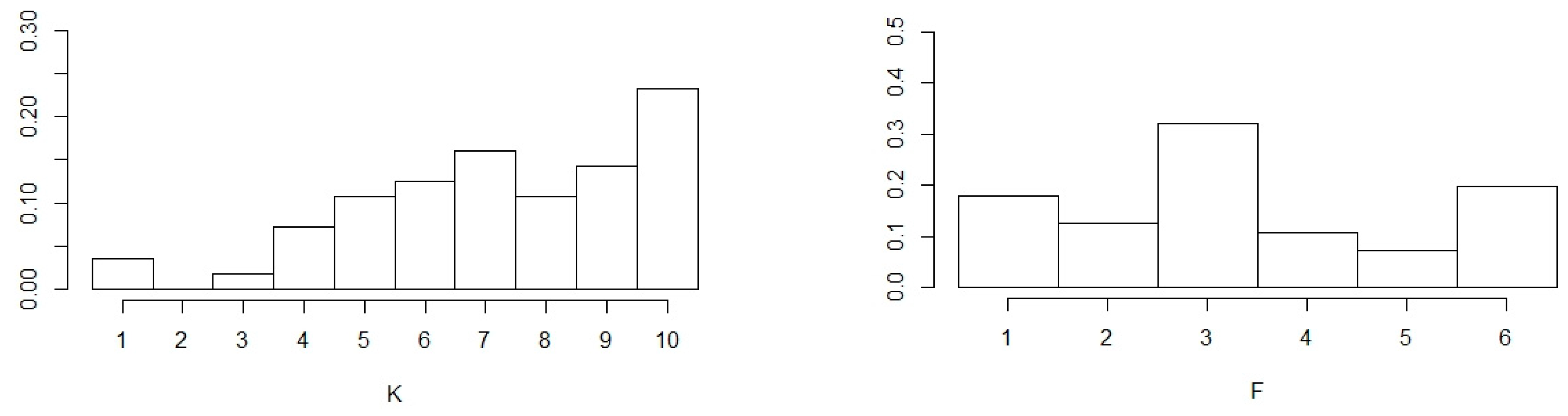
Figure 1. The selected parameters for BSR.
Ijfs 12 00034 g001
Figure 2. The Giacomini−Rossi fluctuation test. (Different colors represent different commodities.).
Ijfs 12 00034 g002
Figure 3. Frequency of being an important price predictor amongst energy commodities (BSR av EW rec on the left and DMA on the right).
Ijfs 12 00034 g003
Figure 4. Frequency of being an important price predictor amongst food commodities (BSR av EW rec on the left and DMA on the right).
Ijfs 12 00034 g004
Figure 5. Frequency of being an important price predictor amongst materials commodities (BSR av EW rec on the left and DMA on the right).
Ijfs 12 00034 g005
Figure 6. Frequency of being an important price predictor amongst metals commodities (BSR av EW rec on the left and DMA on the right).
Ijfs 12 00034 g006
Figure 7. Number of important price predictors (BSR av EW rec on the left and DMA on the right).
Ijfs 12 00034 g007
Table 1. Most important determinants of commodity prices (except supply, demand, and stocks).
Crude OilNatural GasCoalMetalsAgricultural Commodities
  • economic boost in Asia
  • economic growth
  • exchange rates
  • financialisation of the market
  • interest rates
  • crude oil prices
  • economic growth in Asian countries
  • geographical conditions
  • nature of gas price mechanisms
  • trade agreements and infrastructure
  • weather and climate conditions
  • crude oil and gas prices
  • economic growth
  • interest rates
  • past market liberalisation in China
  • economic conditions (inflation, exchange rates) of main importers and producers
  • global macroeconomic conditions
  • market sentiments
  • cost of fertilizers
  • crude oil prices
  • demand for biofuels
  • energy prices
  • farm prices
  • harvest area
  • interest rates
  • international trade agreements and policies
  • population growth
  • weather and climate conditions
Table 2. The list of explanatory variables.
AbbreviationDescription
dprDividend-to-price ratio
pePrice earnings ratio
strShort-term interest rate
ltr_USLong-term interest rate for the U.S.
ltr_EULong-term interest rate for the Euro area
tsTerm spread
drsDefault return spread
cpiU.S. Consumer Price Index for all urban consumers
ppiU.S. Producer Price Index
ipU.S. industrial production
eeU.S. average hourly earnings of production and nonsupervisory employees
M1M1 money stock for U.S.
M2M2 money stock for U.S.
geaKillian’s Index of Global Real Economic Activity
uneU.S. unemployment rate
AUDAustralian dollar to U.S. dollar exchange rate
CADCanadian dollar to U.S. dollar exchange rate
INRIndian rupee to U.S. dollar exchange rate
reer_AUDReal effective exchange rate based on manufacturing Consumer Price Index for Australia
reer_CADReal effective exchange rates based on manufacturing Consumer Price Index for Canada
reer_INRReal effective exchange rates based on manufacturing Consumer Price Index for India
reer_USReal effective exchange rates based on manufacturing Consumer Price Index for U.S.
tb_USU.S. trade balance
GSCIS&P GSCI Commodity Total Return Index
oi_USDDollar open interest
t_indWorking’s dollar T-index
VXOVXO index (implied volatility based on 30-day S&P 100 index at-the-money options)
GPRGlobal Geopolitical Risk Index (The Benchmark GPR Index)
stocks_USS&P 500 Index
stocks_WorldMSCI WORLD for developed markets index
stocks_G7MSCI G7 index
stocks_EUMSCI EU index
stocks_EMMSCI EM for emerging markets index
stocks_CNHang Seng Index and Shanghai Composite Index glued and rescaled (in December 1990)
ts_BRICSThe share of BRIC countries trade in the total global trade
li_USLeading indicator for U.S.
li_G7Leading indicator for G7 countries
li_EULeading indicator for the euro area
li_CNLeading indicator for China
Table 3. Estimated models.
AbbreviationDescription
BSR recBayesian symbolic regression (recursive)
BSR av MSE recBayesian symbolic regression (recursive) with averaging and weights inversely proportional to MSE
BSR av EW recBayesian symbolic regression (recursive) with equal weights
GP recSymbolic regression with genetic programming (recursive)
BSR fixBayesian symbolic regression (fixed parameters)
BSR av MSE fixBayesian symbolic regression (fixed parameters) with averaging and weights inversely proportional to MSE
BSR av EW fixBayesian symbolic regression (fixed parameters) with equal weights
GP fixSymbolic regression with genetic programming (fixed parameters)
DMADynamic Model Averaging with Occam window
BMABayesian Model Averaging with Occam window
DMA 1VDynamic Model Averaging over one-variable component models
DMS 1VDynamic Model Selection over one-variable component models
BMA 1VBayesian Model Averaging over one-variable component models
BMS 1VBayesian Model Selection over one-variable component models
LASSOLASSO regression (recursive)
RIDGERIDGE regression (recursive)
ENElastic net regression (recursive)
B-LASSOBayesian LASSO regression (recursive)
B-RIDGREBayesian RIDGE regression (recursive)
LARSLeast-angle regression
TVPTime-Varying Parameters regression with forgetting factor equal to 1
TVP fTime-Varying Parameters regression with forgetting factor equal to 0.99
ARIMAAutomatic ARIMA (recursive)
HAHistorical average
NAÏVENo-change method
Table 4. nRMSE of the estimated models.
BSR recBSR av MSE recBSR av EW recGP recBSR fixBSR av MSE fixBSR av EW fixGP fixDMABMADMA 1VDMS 1VBMA 1VBMS 1VLASSORIDGEENB-LASSOB-RIDGRELARSTVPTVP fARIMAHANAIVE
Brent0.09920.08480.08400.10990.09690.08240.08820.09240.07210.07380.07510.07490.07420.07420.07780.08150.07740.07610.07810.07740.08700.08750.08770.64980.0925
Dubai0.08420.07610.07660.10970.15760.09800.09090.09080.06780.06860.07070.07060.07000.07000.07330.07810.07430.07250.07450.08150.08330.08340.08430.66470.0908
WTI0.11131047.64660.09370.10410.11753264.90702771.78260.13520.07760.07550.07680.07660.07600.07600.07900.08370.07920.07940.08160.07980.08980.09280.09050.60290.0947
Coal_AU0.10360.11020.10870.09550.10634014.93550.60560.15650.09210.09460.09940.10080.09980.09980.09260.09360.09250.09270.09190.09830.10380.10920.10270.54900.0994
Coal_ZA0.09250.08080.07860.08510.09550.08930.08780.08390.08550.08710.08550.08510.08460.08380.08100.08220.08130.08150.08080.08260.08850.08690.08210.54230.0872
Gas_US0.18410.18721.62130.48690.182141,824.361471,166.56001.18440.17420.17430.17900.17850.17540.17520.17800.18380.17860.17980.18160.17850.20330.21310.18540.59500.1812
Gas_EU0.08740.16350.08620.08940.594417.948036,101.12640.28500.07510.07710.08060.07990.08040.08020.07550.07600.07550.07650.07670.07880.08250.09630.07560.59840.0839
Gas_JP0.06076756.00106756.00100.05950.135513,511.982328,114.60240.10180.05460.05520.05670.05620.05850.05910.08750.05900.05890.05690.05830.08220.10100.10580.05520.57760.0586
Cocoa0.06170.05870.05860.07040.10780.06120.06110.30080.05850.05740.05840.06130.05810.05820.05850.05940.05910.05800.05790.05850.07720.08490.05720.37690.0578
Coffee_Arabica0.08860.07500.07400.09250.33300.13680.08090.07680.07380.07540.07550.08080.07510.07780.07580.07590.07570.07420.07410.07990.08580.09920.07400.38180.0741
Coffee_Robusta0.754435,128.298060,851.92780.418849,684.2213167,366.9005182,580.92620.06920.05560.05970.05620.05830.05660.05720.05990.05760.05900.05600.05680.06290.06630.06560.05500.33410.0559
Tea_Colombo0.05590.05300.05260.09060.06660.06420.06660.06020.05880.05020.05240.05350.05110.05150.05070.05180.05070.05120.05140.05090.10270.13490.05080.37430.0508
Tea_Kolkata0.12830.12710.12600.14610.13840.12070.12060.12700.15100.12010.12700.12880.12690.12800.12660.12730.12690.12640.12710.12870.15180.68580.12150.26540.1270
Tea_Mombasa0.08690.06760.09990.07720.076381,392.4276130.04890.20880.06870.06750.06880.06950.06790.06860.06810.06850.06840.06810.06810.07290.23470.22290.06850.28420.0680
Coconut_oil0.11170.09020.08990.11680.10880.09470.09540.09750.08790.08700.08900.09000.08900.08880.08970.09010.09010.09010.09060.09030.10120.10430.08950.49500.0910
Groundnuts0.06650.06370.06430.09870.07750.08210.06940.18280.05820.06120.06240.06280.06330.06560.06310.06320.06320.06300.06280.06380.07900.07520.05960.34580.0629
Fish_meal53.45230.194225.477453.38460.1465106.7756141.31780.05630.05630.05570.05600.05830.05550.05630.05560.05530.05550.05500.05500.05930.06270.07050.05700.50680.0550
Palm_oil0.13800.192384.13730.0753382.0911188.14130.24270.15000.06360.06600.06630.06600.06680.06740.06790.06860.06930.06750.06820.07280.07800.08060.06340.41600.0685
Soybeans0.08941.500412.5538346.53960.09021.7229219.17010.06200.05840.05770.05950.06070.05880.05970.05860.05880.05850.05890.05970.05900.06690.06870.05930.36990.0598
Soybean_oil0.05580.05610.05600.06220.05900.05660.05630.26190.05220.05410.05430.05530.05540.05580.05560.05500.05500.05500.05540.05530.06220.07180.05260.41720.0568
Soybean_meal0.06950.06150.06130.07730.09650.06760.06880.06640.06220.06220.06240.06340.06230.06340.06240.06220.06220.06200.06220.06340.07380.09050.05830.39900.0622
Maize0.07520.07130.07100.13800.10180.07960.08220.27670.07110.07140.07200.07290.07220.07260.07130.07120.07140.07180.07180.07220.07840.08600.07180.42520.0725
Rice_50.08660.07860.07821.02940.10640.08820.087110.56960.08440.07740.07760.07820.07680.07830.07800.07740.07770.07670.07570.08730.08700.09140.07490.38290.0755
Rice_1000.08780.07930.07800.08820.15550.08440.08640.07840.08270.07800.07880.07970.07810.07980.08190.07940.08000.07920.08000.08660.08890.11080.07930.45230.0768
Wheat_SRW0.08230.08050.08060.10560.11180.08320.08280.08300.08090.07970.08120.08290.08100.08140.08090.08110.08080.08090.08090.08190.08850.09250.07950.36940.0804
Wheat_HRW0.07810.07510.07500.07840.08950.08440.09260.08630.07750.07420.07530.07570.07510.07560.07540.07520.07520.07490.07520.07820.08240.08670.07440.37140.0746
Banana0.09610.09470.09440.16770.10300.09760.10850.44570.09120.09170.09300.09720.09230.09380.09240.09180.09220.09220.09170.09220.12100.12490.09190.39930.0915
Orange0.528777,708.5698109,896.51860.29580.1121495,972.8294544,551.3422747.49200.11140.11190.11330.11550.11270.11270.11360.11240.11380.11240.11210.11440.13580.15110.11060.35710.1120
Beef0.04970.04850.04880.05070.14510.05060.04960.08590.04760.04780.04840.04860.04830.04850.04830.04870.04870.04870.04890.04940.05260.05500.04560.37680.0487
Chicken0.04840.04650.04600.04830.04740.04550.04560.04650.04570.04540.04610.04630.04580.04570.04600.04620.04610.04650.04690.04690.04820.05210.04350.26190.0460
Shrimps0.04450.04340.04320.05220.04760.04670.04780.07190.04210.04260.04290.04390.04310.04340.04290.04300.04300.04280.04290.04690.05350.05310.03920.19300.0428
Sugar_EU0.03460.03230.03230.04010.03850.03450.03330.07840.03260.03220.03420.03390.03390.03390.03220.03210.03220.03280.03280.03310.03920.03870.03400.24820.0325
Sugar_US0.04170.04130.04160.04220.04170.04150.04130.04190.04300.04060.04170.04220.04100.04080.04210.04160.04210.04170.04150.04350.04400.04440.04000.21060.0413
Sugar_World162.31360.16530.26840.1072195,035.8825283,162.9708516,035.53250.60070.08250.08180.08280.08660.08240.08280.08210.08260.08240.08220.08220.08190.09330.09810.07800.41360.0821
Tobacco0.02420.01710.01710.02020.04580.02960.02550.02010.01670.01780.01660.01710.01710.01740.01860.01780.01840.01680.01710.01820.02160.02260.01620.23790.0165
Logs_CM0.03420.03160.03180.03610.03840.03710.03700.05940.03200.03040.03200.03240.03180.03220.03200.03260.03220.03170.03210.03440.03680.04340.03170.22940.0328
Logs_MY0.0661458.1314323.94750.17410.03700.17220.03540.04610.03190.03370.03320.03380.03330.03360.03340.03320.03340.03310.03300.04440.04280.04610.03080.23900.0330
Sawnwood0.02710.02690.02690.12050.04270.03480.03060.15230.02440.02480.02600.02770.02600.02640.02630.02600.02610.02620.02660.02680.03520.03520.02590.20060.0258
Plywood0.02840.07590.10580.03840.0389112.6283424.01290.03790.02190.02240.02270.02390.02290.02360.02330.02240.02300.02230.02230.02800.03100.03480.02220.15410.0222
Cotton0.08440.09345.79910.08060.0889116,060.2346267.73860.14110.07780.07900.07820.07870.07780.07790.08080.07910.08070.07840.07890.07930.08160.08450.06380.32930.0769
Rubber0.11180.09950.10030.11990.22250.13720.10980.10140.10430.09830.10220.10550.10130.10110.10220.10070.10140.10160.10270.10270.11030.11020.09950.61440.1016
Phosphate_rock0.20180.19230.19180.19430.19350.19300.19240.19150.22530.19510.19250.19250.19250.19250.19890.19540.19540.19890.20470.23310.20760.25020.23930.86010.1934
Dap0.1093250.04930.59550.11071.8048532.8508569.07500.21110.09980.10100.10110.10200.10190.10140.10020.09770.09720.09990.10100.10270.10240.10200.09420.57900.1042
Tsp0.10790.10750.10590.11570.13990.11860.11920.11400.10240.11370.11020.10990.11390.11270.10670.10440.10530.10620.10580.11000.11100.11090.09470.63950.1147
Urea0.15590.14240.14690.23340.29020.18120.24120.14260.14870.14450.15290.15040.15200.15370.15220.15230.15200.15100.15260.15330.17220.17620.14830.58290.1524
Potash0.12390.11510.11490.12770.12660.11660.11530.11480.11700.11420.11510.11510.11450.11450.11530.11570.11610.11510.11470.12180.11650.11960.12710.62990.1142
Aluminium0.05700.04710.04720.06310.06630.06460.05400.05150.04390.04560.04660.04630.04690.04800.04590.04680.04600.04630.04680.04610.05570.05680.04990.23510.0508
Iron0.11120.11110.11060.11270.11470.11400.11390.12060.11860.12180.11900.11890.12010.12010.11490.10970.11150.11130.11080.11440.16210.12150.11260.69990.1148
Copper0.07090.06920.06960.07650.12730.08520.08200.22310.06660.06750.06870.07070.06830.06790.06860.06950.06860.06860.06950.07220.07680.07970.07020.57060.0718
Lead0.08990.08310.08360.09780.18030.10500.10810.08610.08470.08210.08390.08520.08300.08250.08460.08490.08420.08390.08520.08350.09330.09890.08180.59830.0845
Tin0.07110.07110.07090.07430.07620.07550.07630.13000.06830.07030.07100.07160.07090.07120.07200.07110.07100.07070.07140.07170.07420.08130.07170.61200.0735
Nickel0.11140.11060.11060.12970.11280.11680.11720.25890.10480.11050.11080.11240.11070.11070.11000.11060.11010.10970.10980.11250.11870.11500.10400.58370.1110
Zinc0.07370.07510.07540.08140.15480.07860.07920.22730.07430.07430.07420.07420.07380.07340.07680.07520.07690.07460.07500.07830.08770.09350.07380.46520.0761
Gold0.04150.04180.04210.04220.04470.04430.04360.05840.04130.04060.04120.04270.04180.04240.04640.04670.04640.04130.04190.04480.05220.04900.04210.64760.0418
Platinum0.08190.06330.06280.06440.09490.06760.06890.06640.06560.06200.06390.06360.06420.06430.06250.06260.06280.06280.06290.06550.07120.07140.06640.51910.0664
Silver0.09261.04620.14730.08950.211421,752.57828168.06940.28190.09000.08900.08970.08900.08960.08950.09000.09010.08990.08970.09080.09070.11780.10430.09120.69780.0915
Table 5. Outcomes of the MCS procedure over out-of-sample period.
ModelFrequency
ARIMA65.45%
DMA60.00%
BMA56.36%
NAIVE25.45%
BMS 1V18.18%
BMA 1V16.36%
BSR av MSE rec14.55%
BSR av EW rec14.55%
B-LASSO14.55%
B-RIDGRE14.55%
RIDGE12.73%
EN12.73%
BSR rec10.91%
BSR av EW fix10.91%
DMA 1V10.91%
DMS 1V10.91%
LASSO9.09%
LARS9.09%
GP fix7.27%
GP rec5.45%
BSR av MSE fix5.45%
TVP3.64%
TVP f3.64%
BSR fix0.00%
HA0.00%
Disclaimer/Publisher’s Note: The statements, opinions and data contained in all publications are solely those of the individual author(s) and contributor(s) and not of MDPI and/or the editor(s). MDPI and/or the editor(s) disclaim responsibility for any injury to people or property resulting from any ideas, methods, instructions or products referred to in the content.

