Large-Scale Empirical Tests of the Markov Tree Model

Abstract

The Markov Tree model is a discrete-time option pricing model that accounts for short-term memory of the underlying asset. In this work, we compare the empirical performance of the Markov Tree model against that of the Black-Scholes model and Heston’s stochastic volatility model. Leveraging a total of five years of individual equity and index option data, and using three new methods for fitting the Markov Tree model, we find that the Markov Tree model makes smaller out-of-sample hedging errors than competing models. This comparison includes versions of Markov Tree and Black-Scholes models in which volatilities are strike- and maturity-dependent. Visualizing the errors over time, we find that the Markov Tree model yields more accurate and less risky single instrument hedges than Heston’s stochastic volatility model. A statistical resampling method indicates that the Markov Tree model’s superior hedging performance is due to its robustness with respect to noise in option data.

1. Motivation

The Markov Tree (MT) model, introduced in our past work [1,2], is a discrete-time option pricing model that accounts for short-term memory of the underlying asset. The MT model generalizes the binomial tree model. In the binomial tree model, the underlying asset’s log returns follow a random walk: at each time step, the asset flips the same biased coin to decide whether to increase or decrease.

In the MT model, the underlying asset’s log returns follow a delayed random walk. There are two coins, a “+” coin and a “−” coin, each with potentially different biases and different associated increments. If the asset decreased (respectively, increased) in value at step n, then at step $n+1$, we flip the “−” (respectively, “+”) coin. The increment at step $n+1$ thus depends on the identity of the coin that we flip at step $n+1$, which itself depends on the result from step n. This first-order Markovian dependence on the past is what gives the MT model its name.

When we actually price an option using the MT model, we use an asymptotic approximation of the exact Markov tree price [2]. We do this because the approximation is both extremely accurate and orders of magnitude faster than computing prices with a large, discrete Markov tree. The MT asymptotic approximation formula we employ is a perturbation of the classical Black-Scholes formula [3]. We may view this perturbation as incorporating the effects of short-term memory in the underlying asset.

When researchers have sought to generalize the Black-Scholes model, a main focal point has been the assumption of constant volatility. Because volatility governs the dynamics of the underlying asset, if we assume it is constant, then it should not depend on option parameters such as strike price and expiration date. This logic is inconsistent with empirical observations such as the volatility smile. This has led to the development of stochastic volatility (SV) models, in which the volatility follows a stochastic process. Within this class of models, we focus our attention on the Heston model [4], an SV model that admits a closed-form price.

In this paper, we use market data to conduct extensive tests of the MT model. The purpose of these tests is to answer the following central question: which feature is more important to include in an option pricing model, short-term memory of the underlying asset or stochastic volatility? In our view, the true test of an option pricing model is its out-of-sample hedging performance; this view is in line with recent work that details multiple advantages of hedging tests as compared with pricing tests [5]. Therefore, to answer the central question, we compare the out-of-sample hedging performance of the MT model against the Black-Scholes and Heston models. For consistency with the literature on empirical testing of option pricing models, we also compare in-sample and out-of-sample pricing results.

The MT model is one of several published models that account for memory in the underlying asset [6,7,8,9,10,11,12,13]. Within this set of models, there are two reasons why the MT model is the simplest: (i) the model requires the estimation of only three parameters; and (ii) the MT model is fundamentally a discrete-time model, allowing us to bypass the technical difficulties of estimation and filtering for stochastic delay/functional differential equations. Increasing the complexity of the model may well enable better agreement with observed memory dynamics. To our knowledge, no option pricing model with memory has been subjected to large-scale empirical tests. It is statistically sound to begin the empirical investigation of such models by examining a relatively simple, parsimonious example, i.e., the MT model.

We are aware of the deep development of SV models. There are two reasons for choosing the Heston model as a representative SV model. First, the Heston model has already been subjected to pricing and hedging tests [14,15,16,17,18,19]. Comparing MT-versus-Heston results with this literature, we can gauge how the MT model would perform against many other models. Second, the problem of fitting the Heston model to market data has received much more attention than the corresponding problem for other SV models. Using one of the established methods for fitting the Heston model, we are able to study the performance of this SV model on a large data set in a reasonable amount of time.

1.1. Summary of Present Work

In the present study, we use a large database of both individual equity options and index options to study the out-of-sample pricing and hedging performance of the MT, Heston, and Black-Scholes models.

We use two databases of historical option prices. The first consists of 20,050 S&P 500 index call options from 1 January 2009 to 31 December 2010. The second consists of 3,483,461 unique LIFFE Paris equity call options traded between 19 September 2009 and 18 June 2012. Using this data, we calculate and compare the out-of-sample hedging errors made by the Black-Scholes, Heston, and MT models.

In order to conduct these tests, we develop three new methods for fitting the MT model to data, a problem that we frame as a nonlinear regression problem. The first two regression methods we develop are, respectively, underconstrained and overconstrained least-squares methods. The third method is a robust regression method that uses a loss function that smoothly approximates the $L^1$/absolute loss function.

1.2. Results

Our primary result is that using any of the three regression methods developed in this paper, the MT model yields better out-of-sample hedging performance than either the Black-Scholes or Heston models. This comparison includes the practitioner’s version of the Black-Scholes model in which volatility is allowed to depend on option strike and maturity, as well as a version of the Black-Scholes model, often used in the empirical option pricing literature, in which volatility is independent of option strike and maturity.

For the overconstrained least-squares MT method, we analyze the regression residuals and show that they fit a generalized hyperbolic (GH) distribution with heavier-than-Gaussian tails. We then develop computational bootstrap procedures to better understand how the MT model is likely to perform in the future. Here we add noise to market option prices, either by sampling from the best-fit GH distribution or by resampling regression residuals, and we rerun our hedging tests using this simulated option data. Using both bootstrapping approaches, we compute the distribution of the difference between the absolute errors committed by the Heston and MT models. The results show that the MT model leads to more accurate and less risky hedges.

We conclude from these results that if one seeks to extend the Black-Scholes model, accounting for short-term memory of the underlying asset may be just as important as accounting for stochastic volatility.

Further insights obtained from this study are described in Section 9.

1.3. Prior Work

The literature on option pricing is vast and has been surveyed elsewhere [20,21,22]. We focus our attention on work that empirically tests the hedging performance of one or more of the models studied in this paper.

The MT and Black-Scholes models have been compared in prior work. The first test considered short- and mid-term European call options on six different stocks that were components of the CAC-40 index. Across 44 days of testing, the MT model outperformed the Black-Scholes model in out-of-sample pricing [1]. The second test considered American call options on 89 stocks that were components of the S&P 100 index. In 10 days of testing, the MT model outperformed the Black-Scholes model in aggregate out-of-sample pricing [2].

Previous work on the MT model did not explore sufficiently the different methods for fitting the model to data, instead relying on ad hoc procedures based on historical volatilities [1,2]. While these studies did consider genuine out-of-sample tests of pricing errors, the issue of hedging errors was left unaddressed. Prior work on the MT model compared its predictions only to those of the Black-Scholes model, leaving out comparisons to more sophisticated models such as SV models. Finally, the sample sizes of previous empirical studies of the MT model are much smaller than that of the present study.

A comparison of the hedging performance of the Black-Scholes, Heston, and Brigo-Mercurio models has been carried out [23]. The Brigo-Mercurio formula [24] is similar to the asymptotic approximation of the exact MT option price: both price a vanilla call option using a risk-neutral distribution that consists of a mixture of normals. However, the Brigo-Mercurio model differs from the MT model in one key aspect: it does not explicitly account for short-term memory of the underlying asset. Consequently, the variances of the mixture components in the Brigo-Mercurio model have no interaction with one another; each variance is a function of a distinct model parameter. In the MT model, the variances of both mixture components interact strongly with one another; each variance is a function of the same two model parameters. The Brigo-Mercurio model allows for an arbitrary number of mixture components, while the MT model allows for only two. When we restrict the Brigo-Mercurio model to two mixture components, the option price is a function of four model parameters [23] rather than three for the MT model [1].

These differences may serve to explain why the particular Brigo-Mercurio model tested in earlier work showed poorer hedging performance than either the Black-Scholes or Heston models [23]. This contrasts sharply with the results presented in this paper.

The MT model is an example of a discrete-time Markov chain option pricing model. A recent study explores a continuous-time Markov chain model, including results on numerical simulation together with estimation of parameters [25]. As is typical in this literature, [25] avoids pursuing out-of-sample hedging performance and/or a large-scale empirical test using market prices of options.

Several authors have compared the hedging performance of stochastic volatility, jump diffusion, and Black-Scholes models [5,26,27,28,29,30,31]. While this literature does include comparisons between varieties of stochastic volatility models, it is important to note that none of these papers test constant volatility models that are more complex than Black-Scholes. The question of whether a constant volatility model might outperform stochastic volatility models in a large-scale (i.e., millions of options), out-of-sample hedging test has not been answered.

There does exist prior empirical work analyzing individual equity option data. One of the earliest such works [32] applies nonparametric tests to Chicago Board of Exchange (CBOE) individual equity option data to check for systematic differences between Black-Scholes and market prices. A later study [33] examines a nearly two-year span of CBOE option data on 10 stocks to test implications of the Hull-White stochastic volatility model [34].

A more recent study analyzed market data for options written on the S&P 100 index and the stocks that form its 30 largest components [35]. Using 350,000 distinct option quotes (both calls and puts), this study examines the differences between implied risk neutral distributions for index and individual equity options. The effect of variables such as the price-to-earnings ratio and market capitalization on the skewness of implied risk neutral distributions has been studied using four years of end-of-week option data for 856 unique firms [36]—this data set comprises 67,910 distinct option quotes.

Multiple studies have used individual equity option data to analyze various models for the implied volatility smile [37,38,39]—these studies each use between 14,120 and 400,000 distinct option quotes.

In this paper, we analyze a data set that is an order of magnitude larger than the largest of the data sets we have seen mentioned in the literature. Furthermore, we compute hedging errors for individual equity options, unlike all prior studies we have reviewed that use market data for such options.

2. Option Pricing Models

For a given option, let K denote the strike price, T the time in years to expiration, r the risk-free rate of interest, and $S_0$ the spot price of the underlying asset. We denote the option price as a function of the form $F(\mathbf{x},\beta )$, where $\mathbf{x}=[K,T,r,S_0]$ and β is a vector of model parameters that must be statistically estimated from data. Typically, these model parameters include one or more volatilities.

We define moneyness as $m=S_0/K$, and maturity as the time to expiration in days.

Let us now review three classes of models. All models that we discuss treat r as constant over the life of the option.

2.1. Black-Scholes

The underlying asset price $S_t$ at any time t is assumed to follow the SDE

$$d{S}_t={\mu }_{\mathrm{BS}}{S}_{t}dt+{\sigma }_{\mathrm{BS}}{S}_{t}d{W}_t,$$

(1)

where ${\mu }_{\mathrm{BS}}$ and ${\sigma }_{\mathrm{BS}}$ are constants and $W_t$ is the standard Wiener process. The annualized volatility ${\sigma }_{\mathrm{BS}}$ is assumed to be constant. The Black-Scholes European call option price is

$$\begin{array}{c}{F}^{\mathrm{BS}}(\mathbf{x},{\beta }^{\mathrm{BS}})=\Phi \left(d_1\right)S_0-\Phi \left(d_2\right)Kexp(-rT),\end{array}$$

(2)

$$\begin{array}{c}{d}_1=\frac{log(S_0/K)+(r+{\sigma }_{\mathrm{BS}}^2/2)T}{{\sigma }_{\mathrm{BS}}\sqrt{T}},d_2=d_1-{\sigma }_{\mathrm{BS}}\sqrt{T},\end{array}$$

(3)

where Φ is the standard normal cumulative distribution function.

The Black-Scholes model is a one-parameter model with ${\beta }^{\mathrm{BS}}={\sigma }_{\mathrm{BS}}$.

2.2. Heston

In Heston’s stochastic volatility model, the underlying asset $S_t$ is governed by the coupled system

$$\begin{array}{cc}\hfill d{S}_t& =r{S}_{t}dt+\sqrt{v_t}{S}_{t}d{W}_t^s,\hfill \end{array}$$

(4)

$$\begin{array}{cc}\hfill d{v}_t& =\kappa (\theta -v_t)dt+\xi \sqrt{v_t}d{W}_t^v,\hfill \end{array}$$

(5)

where $v_t$ is the instantaneous variance of the asset price, $d{W}_t^s$ and $d{W}_t^v$ are Wiener processes with correlation $\rho dt$, θ is the long-term variance, κ is the rate at which $v_t$ reverts to θ, and ξ is the volatility of the volatility. The Heston model contains five parameters, i.e., ${\beta }^{\mathrm{SV}}=(v_0,\rho ,\theta ,\kappa ,\xi )$. The closed form European call option price is [40]:

$$F^{\mathrm{SV}}(\mathbf{x},{\beta }^{\mathrm{SV}})=S_0{P}_1-K{e}^{-rT}{P}_2,$$

(6)

where

$$\begin{array}{c}{P}_1=\frac{1}{2}+\frac{1}{\pi }{\int }_0^{\infty }\mathrm{Re}\left(\frac{e^{-i\omega logK}\varphi (\omega -i)}{i\omega \varphi (-i)}\right)d\omega \\ P_2=\frac{1}{2}+\frac{1}{\pi }{\int }_0^{\infty }\mathrm{Re}\left(\frac{e^{-i\omega logK}\varphi \left(\omega \right)}{i\omega }\right)d\omega \\ \varphi \left(\omega \right)=e^A{e}^B{e}^C\end{array}$$

and

$$\begin{array}{cc}\hfill A& =i\omega (log{S}_0+rT)\hfill \\ \hfill B& =\frac{\theta \kappa }{{\xi }^2}\left((\kappa -\rho \xi i\omega -d)T-2log\left(\frac{1-g_2{e}^{-dT}}{1-g_2}\right)\right)\hfill \\ \hfill C& =\frac{\frac{v_0}{{\xi }^2}(\kappa -\rho \xi i\omega -d)(1-e^{-dT})}{1-g_2{e}^{-dT}}\hfill \\ \hfill d& =\sqrt{{(\rho \xi i\omega -\kappa )}^2+{\xi }^2(i\omega +{\omega }^2)}\hfill \\ \hfill g_2& =\frac{\kappa -\rho \xi i\omega -d}{\kappa -\rho \xi i\omega +d}.\hfill \end{array}$$

2.3. Markov Tree

For $k\in \{-1,0,1\}$, let $Z_k$ be a discrete random variable that achieves the outcomes $\{l_k,-l_k\}$ with probabilities $\{q_k,1-q_k\}$. Then, as originally proposed [1], the MT model assumes the underlying asset price $S_n$ follows the persistent (or delayed) random walk

$$\begin{array}{cc}\hfill n=1& :log{S}_1=log{S}_0+Z_0\hfill \end{array}$$

(7a)

$$\begin{array}{cc}\hfill n\ge 1& :log{S}_{n+1}=log{S}_n+\left\{\begin{array}{cc}{Z}_1\hfill & S_n\ge S_{n-1}\hfill \\ Z_{-1}\hfill & S_n<S_{n-1}\hfill \end{array}\right..\hfill \end{array}$$

(7b)

Note that this process generalizes the random walk in the binomial option pricing model (BOPM). In the BOPM, the increments of the process are independent and identically distributed (i.i.d.) samples of a fixed random variable, while in Equation (7), the increments of the process follow a first-order Markov chain.

This process generates a risk-neutral probability mass function (pmf); using asymptotic analysis in an appropriate continuous-time limit, this pmf can be approximated closely by a mixture of normal densities, resulting in the following expression for the price of a European call option [2]:

$$\begin{array}{c}{F}^{\mathrm{MT}}(\mathbf{x},{\beta }^{\mathrm{MT}})e^{rT}=q_0{S}_{0}exp\left(\frac{{\sigma }_1^2}{2}+{\mu }_1\right)\Phi \left(x_1\right)\hfill \\ \hfill +(1-q_0)S_{0}exp\left(\frac{{\sigma }_2^2}{2}+{\mu }_2\right)\Phi \left(x_2\right)-q_{0}K\Phi \left(x_3\right)-(1-q_0)K\Phi \left(x_4\right),\end{array}$$

(8)

where

$$x_i=\frac{{\mu }_i+{\sigma }_i^2+log(S_0/K)}{{\sigma }_i},x_{i+2}=\frac{{\mu }_i+log(S_0/K)}{{\sigma }_i}$$

(9

for $i\in \{1,2\}$. In this paper, we treat Equation (8) as the MT model’s option price.

The MT model is a three-parameter model with ${\beta }^{\mathrm{MT}}=(\sigma ,{\sigma }_{+},{\sigma }_{-})$. The parameters $q_k$, $l_k$, ${\sigma }_1$, and ${\sigma }_2$ that appear either in the stochastic process Equation (7) or on the right-hand sides of Equations (8) and (9) are all functions of the components of ${\beta }^{\mathrm{MT}}$—see Appendix A for detailed algebraic expressions of these quantities.

3. Regression

We now describe how we use market data to fit the three models described in Section 2.

Let $V_{\Theta ,i}$ denote the column vector of all option prices associated with the symbol Θ on day i. Each row of $V_{\Theta ,i}$ corresponds to a particular option contract, and each such contract corresponds to a row vector of the form ${\mathbf{x}}_j^{\Theta ,i}=(K,T,r,S_0)$. Let $X^{\Theta ,i}$ denote the matrix obtained by stacking these row vectors vertically, i.e.,

$$X^{\Theta ,i}=\left[\begin{array}{c}—{\mathbf{x}}_1^{\Theta ,i}—\\ —{\mathbf{x}}_2^{\Theta ,i}—\\ ⋮\\ —{\mathbf{x}}_{\nu }^{\Theta ,i}—\end{array}\right],$$

where $\nu =|V_{\Theta ,i}|$, the length of $V_{\Theta ,i}$. Let $\mathbf{1}\in {\mathbb{R}}^{\nu }$ denote the column vector $\mathbf{1}={(1,1,\dots ,1)}^{†}$, where † denotes transpose. Then, once we fix the symbol Θ and the day i, the third and fourth columns of $X^{\Theta ,i}$ are, respectively, $r\mathbf{1}$ and $S_0\mathbf{1}$; this is because the spot price of the underlying asset depends only on Θ and i, while the risk-free rate of interest depends only on i.

For the data matrix $X^{\Theta ,i}$, and for each option pricing model $F(\mathbf{x},\beta )$, we let $F(X^{\Theta ,i},\beta )$ denote the result of applying $F(\mathbf{x},\beta )$ to each row of $X^{\Theta ,i}$:

$$F(X^{\Theta ,i},\beta )=\left[\begin{array}{c}F({\mathbf{x}}_1^{\Theta ,i},\beta )\\ F({\mathbf{x}}_2^{\Theta ,i},\beta )\\ ⋮\\ F({\mathbf{x}}_{\nu }^{\Theta ,i},\beta )\end{array}\right].$$

We formulate the nonlinear regression problem

$$V_{\Theta ,i}=F(X^{\Theta ,i},\beta )+{ϵ}_{\Theta ,i},$$

(10)

where ${ϵ}_{\Theta ,i}$ is a column vector of residuals. We now explain how special cases of Equation (10) can be used to fit—that is, determine the values of the regression coefficients β—for each of the option pricing models presented in Section 2.

3.1. Black-Scholes

3.1.1. Overconstrained $L^2$

The Black-Scholes model is a one-parameter model with ${\beta }^{\mathrm{BS}}={\sigma }_{\mathrm{BS}}$. Our first method for finding ${\beta }^{\mathrm{BS}}$ involves using the entire vector $V_{\Theta ,i}$ and the entire data matrix X. We set

$$\begin{array}{cc}\hfill V_{\Theta ,i}& =F^{\mathrm{BS}}(X^{\Theta ,i},\beta )+{ϵ}_{\Theta ,i}\hfill \end{array}$$

(11a)

$$\begin{array}{cc}\hfill {\beta }_{\Theta ,i}^{\mathrm{BS}}& ={argmin}_{\beta \in [0.05,0.95]}\frac{1}{2}{ϵ}_{\Theta ,i}^{†}{ϵ}_{\Theta ,i},\hfill \end{array}$$

(11b)

yielding a volatility ${\sigma }_{\mathrm{BS}}$ that is independent of strike and time to expiration. This is a commonly used approach in prior empirical studies [27,30].

3.1.2. Practitioner’s Black-Scholes

In this second method, we find a different ${\beta }^{\mathrm{BS}}$ for each row of $\left[\begin{array}{cc}{X}^{\Theta ,i}& V_{\Theta ,i}\end{array}\right]$:

$${\left[V_{\Theta ,i}\right]}_j=F^{\mathrm{BS}}({\mathbf{x}}_j^{\Theta ,i},{\sigma }_{\left(j\right)}^{\Theta ,i}).$$

(12)

Here ${\left[V_{\Theta ,i}\right]}_j$ denotes the j-th row of the vector $V_{\Theta ,i}$. There is no error term ϵ, because Equation (12) is a nonlinear scalar equation for the single unknown ${\sigma }_{\left(j\right)}^{\Theta ,i}$ that can be solved almost to machine precision, even when we impose the box constraints $0.05\le {\sigma }_{\left(j\right)}^{\Theta ,i}\le 0.95$.

By solving Equation (12) for each $j=1,2,\dots ,\nu$, we obtain volatilities ${\sigma }_{\left(1\right)}^{\Theta ,i},\dots ,{\sigma }_{\left(\nu \right)}^{\Theta ,i}$ that are functions of both the strike price K and time to expiration T. The ${\sigma }_{\left(j\right)}^{\Theta ,i}$ values obtained in this way are known as implied volatilities. This procedure is one of the methods most commonly used by practitioners for fitting the Black-Scholes model to market data.

To actually carry out the solution for both the overconstrained $L^2$ method and this method, we use the R function optimize, which combines golden section search and interpolation [41].

3.2. Heston

Since ${\beta }^{\mathrm{SV}}$ is five-dimensional, by analogy with linear regression problems, one does not expect the least-squares solution of Equation (10) to be unique unless $V_{\Theta ,i}$ contains at least 5 rows. Therefore, a commonly used technique is to take $V_{\Theta ,i}$ to be all available call option prices for symbol Θ and day i in a particular data set, so that the number of rows ν is always more than 5. The net effect of this is to compute an estimate ${\beta }^{\mathrm{SV}}$ that is strike- and maturity-independent:

$$\begin{array}{cc}\hfill V_{\Theta ,i}& =F^{\mathrm{SV}}(X^{\Theta ,i},\beta )+{ϵ}_{\Theta ,i}\hfill \end{array}$$

(13a)

$$\begin{array}{cc}\hfill {\beta }_{\Theta ,i}^{\mathrm{SV}}& ={argmin}_{\beta \in \mathcal{S}}\frac{1}{2}{ϵ}_{\Theta ,i}^{†}{ϵ}_{\Theta ,i}.\hfill \end{array}$$

(13b)

Here $\mathcal{S}=\{(v_0,\theta ,\rho ,\kappa ,\xi )\in {\mathbb{R}}^5|0.05<v_0<0.95,0.05<\theta <0.95,-0.9<\rho <0.9,1<\kappa <6,0.01<\xi <1.11\}$. Similar box constraints are often used in the literature [40].

The main caveat of applying this procedure lies in the way Equation (13b) is computed. The analytical gradient of the objective function—specifically $F^{\mathrm{SV}}$—is not known, and numerically computed gradients are computationally expensive and inaccurate. This is because the evaluation of $F^{\mathrm{SV}}$ requires the numerical computation of an oscillatory integral. For these reasons, derivative-free rather than gradient-based optimization techniques are used to solve for β [40,42].

Two popular derivative-free techniques that are used to solve Equation (13b) for Heston’s model are the Nelder-Mead algorithm [43,44] and differential evolution [40]. Using artificially created option data from a set of known parameters, [40] shows that differential evolution outperforms other derivative-free optimization techniques. We choose the Nelder-Mead algorithm for two reasons. First, differential evolution requires a prohibitively large number of evaluations of the objective function to achieve reasonable accuracy for a large-scale empirical test. Second, our tests on a subsample of LIFFE option data reveal that using Nelder-Mead with 500 iterations results in better convergence than differential evolution. The specific implementation of the Nelder-Mead algorithm we use is provided by the R function optim [41].

3.3. Markov Tree

We now describe three methods to fit the MT model to data. All three methods are implemented using gradient-based optimization, leveraging the smoothness of the MT model’s option price with respect to the parameters ${\beta }^{\mathrm{MT}}$.

3.3.1. Overconstrained $L^2$

The first method we consider is analogous to the overconstrained procedures described above for the Black-Scholes model and Heston’s stochastic volatility model. Using the full set of market option quotes for symbol Θ and day i, we formulate the regression problem and least-squares solution as

$$\begin{array}{cc}\hfill V_{\Theta ,i}& =F^{\mathrm{MT}}(X^{\Theta ,i},\beta )+{ϵ}_{\Theta ,i}\hfill \end{array}$$

(14a)

$$\begin{array}{cc}\hfill {\beta }_{\Theta ,i}^{\mathrm{MT}}& ={argmin}_{\beta \in \mathcal{B}}\frac{1}{2}{ϵ}_{\Theta ,i}^{†}{ϵ}_{\Theta ,i},\hfill \end{array}$$

(14b)

where $\mathcal{B}=\{(x^1,x^2,x^3)\in {\mathbb{R}}^3|0.05\le x^j\le 0.95,j=1,2,3\}$. This formulation produces an MT volatility vector ${\beta }_{\Theta ,i}^{\mathrm{MT}}$ that does not depend on option strikes and maturities.

3.3.2. Robust MT: Overconstrained Pseudo-Huber

Consider the loss function

$$L\left(x\right)=\delta \left(\sqrt{1+{\left(\frac{x}{\delta }\right)}^2}-1\right),$$

(15)

adapted from the pseudo-Huber loss function ([45] (p. 619)). With δ fixed, $L\left(x\right)$ behaves for small x like the quadratic loss $x^2/\left(2\delta \right)$, while for large x, $L\left(x\right)$ behaves like the absolute loss $\left|x\right|$. In this way, $L\left(x\right)$ gains the absolute loss function’s robustness with respect to outliers. At the same time, $L\left(x\right)$ respects the property that for normally distributed errors (i.e., non-outliers), using the quadratic loss will yield a maximum likelihood estimate. More precisely, a Taylor series expansion of $L\left(x\right)$ about $x=0$ yields

$$L\left(x\right)=\frac{x^2}{2\delta }+O\left(x^4\right).$$

Meanwhile, with δ fixed,

$$\underset{\left|x\right|\to \infty }{lim}\frac{L\left(x\right)}{\left|x\right|}=1.$$

With this loss function, we can formulate an alternative solution to the regression problem Equation (14a), one in which we replace the squared error loss function with $L\left(x\right)$:

$${\beta }_{\Theta ,i}^{\mathrm{MT}}={argmin}_{\beta \in \mathcal{B}}\sum _{j=1}^{\nu }L\left({ϵ}_{\Theta ,i;j}\right),$$

(16)

where ${ϵ}_{\Theta ,i;j}$ is the j-th component of the ${ϵ}_{\Theta ,i}$ vector defined as in Equation (14a). The estimate ${\beta }_{\Theta ,i}^{\mathrm{MT}}$ computed in this way is strike- and maturity-independent.

Unlike the $L^1$ or absolute loss function $\left|x\right|$, for all $\delta >0$ and for all x, $L\left(x\right)$ is smooth, enabling us to use gradient-based optimization to solve Equation (16). We view the resulting solution ${\beta }_{\Theta ,i}^{\mathrm{MT}}$ as a robust solution to the regression problem Equation (14a). In our work, we set $\delta =0.01$.

3.3.3. Practitioner’s MT: Underconstrained $L^2$

As in the practitioner’s Black-Scholes method described in Section 3.1.2, we consider a special case of Equation (10) in which we use only one row of the data matrix $X^{\Theta ,i}$ and the corresponding row of the vector $V_{\Theta ,i}$:

$${\left[V_{\Theta ,i}\right]}_j=F^{\mathrm{MT}}({\mathbf{x}}_j^{\Theta ,i},{\beta }_{\left(j\right)})+{ϵ}_{\Theta ,i}.$$

(17)

Since ${\beta }_{\left(j\right)}^{\mathrm{MT}}$ is three-dimensional, the problem Equation (17) is underconstrained, i.e., the set ${\mathcal{F}}_j=\left\{\beta \right|{\left[V_{\Theta ,i}\right]}_j=F^{\mathrm{MT}}({\mathbf{x}}_j^{\Theta ,i},\beta )\}$ is infinite. For this reason, we treat the nonlinear equation as a constraint, and solve the problem

$${\beta }_{\Theta ,i;j}^{\mathrm{MT}}={argmin}_{\beta \in {\mathcal{F}}_j}{\parallel \beta -\mathbf{b}\parallel }_2^2.$$

(18)

where $\mathbf{b}=(0.5,0.5,0.5)$. This formulation gives a strike- and expiration-dependent set of MT volatilities. One can view this method as a practitioner’s Markov Tree method.

Recall from Section 2.3 that the parameter vector ${\beta }^{\mathrm{MT}}$ can be used to calculate three risk-neutral probabilities ${\left\{q_k\right\}}_{k=-1}^1$. Let $\mathcal{Q}=\{\beta \in {\mathbb{R}}^3|0<q_k\left(\beta \right)<1,-1\le k\le 1\}$. For all index options considered in this study, when we find the solution (18) and insert it into (17), the residual error ϵ is zero to machine precision. We also find that ${\beta }_{\Theta ,i;j}^{\mathrm{MT}}\in \mathcal{Q}$, i.e., the $q_k$’s are valid probabilities.

For approximately ${10}^3$ individual equity options considered in this study, solving Equation (18) results in ${\beta }_{\Theta ,i;j}^{\mathrm{MT}}\notin \mathcal{Q}$. For only these options, we solve the following problem instead of Equation (18):

$${\beta }_{\Theta ,i;j}^{\mathrm{MT}}={argmin}_{\beta \in {\mathcal{F}}_j\cap \mathcal{Q}}{\parallel \beta -\mathbf{b}\parallel }_2^2.$$

(19)

In practice, this produces solutions that satisfy both the ${\mathcal{F}}_j$ and $\mathcal{Q}$ constraints.

3.3.4. Implementation Details

To obtain either of the overconstrained solutions (14b) or (16), we use the L-BFGS-B algorithm [46]. This is a quasi-Newton solver that uses a limited memory (L) version of the BFGS update formula, while also handling box constraints (B). Our use of a quasi-Newton solver means that we avoid calculating the exact Hessian of the objective function. The L-BFGS-B implementation we use is built into the optim command in R [41].

To obtain either of the underconstrained solutions (18) or (19), we use the package nloptr [47], an R interface to the nlopt package [48]. Specifically, we use this package’s implementation of an augmented Lagrangian method [49,50].

For all of the codes/algorithms just mentioned, we pass user-defined functions that use exact formulas to compute the gradient of the MT option price $F^{\mathrm{MT}}$ with respect to ${\beta }^{\mathrm{MT}}$. This gradient is given in detail in Appendix B.

For the overconstrained methods, our results show that at a computed optimum ${\beta }^{\mathrm{MT}}$, the gradient of the objective function is near zero. We also find that either the Hessian at the optimum is positive definite, or the computed optimum lies on the boundary of the feasible set $\mathcal{B}$.

For the underconstrained methods, we rely on the optimization algorithm to single out a unique element of the feasible set. That is, we are less interested in whether the algorithm converges to a local minimum, and more interested in how well the constraints are satisfied. In all of our tests, the solution of either Equation (18) or Equation (19) yields (i) valid risk-neutral probabilities ${\left\{q_k\right\}}_{k=-1}^1$ and (ii) residual errors in Equation (17) that are zero to at least four decimal places, sufficient for the purposes of this study.

4. Tests

In the previous section, we described six procedures for fitting an option pricing model to market data: two Black-Scholes procedures, one stochastic volatility procedure, and three MT procedures. All six procedures can be viewed as special cases of Equation (10). When we evaluate Equation (10) at the optimized value $\beta ={\beta }_{\Theta ,i}$, the resulting value of ${ϵ}_{\Theta ,i}$ will be referred to as the in-sample pricing error.

4.1. Out-of-Sample Pricing Error

Having computed ${\beta }^{\Theta ,i}$, we use this vector of regression coefficients to price options on the symbol Θ on day $i+1$. This leads to the one day out-of-sample pricing error

$$e_{\Theta ,i+1}=V_{\Theta ,i+1}-F(X^{\Theta ,i+1},{\beta }^{\Theta ,i}).$$

(20)

Note that $V_{\Theta ,i+1}$ consists of all available call option prices in our data set for day $i+1$ and symbol Θ. The data matrix $X^{\Theta ,i+1}$ is such that the risk-free interest rate and spot prices are current as of day $i+1$, while the strikes and the expiration dates are read from the call option contracts available on day $i+1$ for symbol Θ.

4.2. Out-of-Sample Hedging Error

Hedging is the process of creating a risk-free portfolio consisting of risky assets. Owing to transaction costs and other financial considerations, a simple and practical form of such a portfolio is one that uses the minimum number of financial instruments [27]. Hedging with a portfolio consisting only of an option and shares of its underlying asset is commonly referred to as single instrument hedging.

Consider a portfolio created by selling one call option at the price $V_{\Theta ,i}^{K,T}$ and buying n shares of its underlying asset at the price of $S_0$ per share. The residual cash obtained through this transaction at time $t=0$ on day i is ${\pi }_{\Theta ,i}^{K,T}=V_{\Theta ,i}^{K,T}-n{S}_0$. The value of this portfolio depends on the market price of the call option and the market price of its underlying asset. A change in the price of the underlying asset at time $t=\Delta t$ leads to a change in the call option price and the value of the portfolio. We seek a portfolio whose value is insensitive to small changes in the underlying asset price. For the BS and MT models, this can be achieved by choosing n such that

$$\frac{\partial {\pi }_{\Theta ,i}^{K,T}}{\partial S_0}=\frac{\partial V_{\Theta ,i}^{K,T}}{\partial S_0}-n=0.$$

Approximating the market price $V_{\Theta ,i}^{K,T}$ by the model price $F({\mathbf{x}}_j^{\Theta ,i},{\beta }^{\Theta ,i-1})$, we have

$$n=\frac{\partial V_{\Theta ,i}^{K,T}}{\partial S_0}\approx \frac{\partial F({\mathbf{x}}_j^{\Theta ,i},{\beta }^{\Theta ,i-1})}{\partial S_0}.$$

(21)

With this n, the portfolio described above with value ${\pi }_{\Theta ,i}^{K,T}$ is often called a delta neutral portfolio. For the MT model, we report the exact forms of n in Appendix C. Since the only stochastic term in the Black-Scholes and MT models is the underlying asset price, for these models, a delta neutral portfolio can be created using a single option and its underlying asset. This cannot be done for a stochastic volatility model, as both the underlying asset price and volatility are stochastic. Therefore, for Heston’s model, and for a portfolio consisting of a call option and shares of its underlying asset, we choose n such that the variance of the portfolio is minimized [27]. This is called a minimum variance hedge.

To evaluate the hedging performance of different models, we first construct a risk-free portfolio at time $t=0$ (day i) consisting of an option (with strike K and time to expiration T) and n shares of its underlying asset (with symbol Θ). To calculate this n, we use Equation (21) with β computed using data on day $i-1$. We invest the residual cash generated into a risk-free bond maturing at time $t=\Delta t$ on day $i+1$. We assess the value of the stock and option at time $t=\Delta t$ (day $i+1$) by closing the portfolio, thereby generating a cash value of $n{S}_{\Delta t}-V_{\Theta ,i+1}^{K,T-\Delta t}$. Maturity of the bond generates another ${\pi }_{\Theta ,i}^{K,T}{e}^{r_i\Delta t}$ on day $i+1$. The hedging error of this self-financed portfolio created on day i and liquidated on day $i+1$ is then

$$H_{\Theta ,i}^{K,T}={\pi }_{\Theta ,i}^{K,T}{e}^{r_i\Delta t}-V_{\Theta ,i}^{K,T-\Delta t}+n_{\mathrm{model}}{S}_{\Delta t}.$$

(22)

5. Data

5.1. LIFFE Paris Individual Equity Options

Market data on electronically traded LIFFE option contracts was obtained from LIFFE, prior to LIFFE’s acquisition first by Euronext and then NYSE. To keep the analysis feasible, we consider only the subset of the data consisting of all LIFFE Paris Equity Options traded between 18 September 2009 and 18 June 2012, encompassing 707 trading days. To further reduce the size of the data set, we only consider call options traded within this period, leaving 7,361,451 unique options. We then apply standard filtering techniques to improve the fitting process for all models, and to remove the bias involved in pricing options with very low trading volume [5]. Specifically, we remove from our data set

• short-term options, i.e., options with maturity strictly less than seven trading days,
• deep in-the-money options (with moneyness $S_0/K\ge 1.4$), and
• deep out-of-the-money options (with moneyness $S_0/K\le 0.8$),

leaving us with 3,483,461 call options in the LIFFE data set. We denote this data set by LIFFE118, since there are options on 118 distinct stocks. The number of unique options in the LIFFE118 data set is approximately 100 times greater than the number of options analyzed in prior empirical hedging studies [26,27,51].

Table 1. For each data set (labeled in boldface), we give the number of options (integer to the left of the semicolon) and their average market price (decimal to the right of the semicolon), binned by moneyness and/or maturity. Rows show different categories of moneyness $m=S_0/K$, and columns separate options by maturity (time to expiration in days). Market prices for LIFFE and SPX options are in Euros (€) and USD ($), respectively.

	<60	60–180	>180	Overall
LIFFE118
<0.94	281,602; 0.31	280,725; 1.05	411,781; 2.60	974,108; 1.49
0.94–0.97	98,580; 0.79	65,437; 2.10	97,078; 4.11	261,095; 2.35
0.97–1	102,438; 1.24	65,866; 2.64	98,096; 4.63	266,400; 2.84
1–1.03	99,652; 1.85	63,418; 3.23	91,491; 5.01	254,561; 3.33
1.03–1.06	92,177; 2.59	59,610; 3.96	86,991; 5.67	238,778; 4.05
>1.06	506,405; 6.46	445,070; 7.95	653,051; 8.98	1,604,526; 7.90
Overall	1,180,854; 3.38	980,126; 4.68	1,438,488; 6.08	3,599,468; 4.81
LIFFE25
<0.94	58,022; 0.26	55,454; 1.01	78,524; 1.82	192,000; 1.11
0.94–0.97	16,829; 0.61	11,843; 1.75	16,207; 2.58	44,879; 1.62
0.97–1	17,217; 0.89	12,177; 2.12	17,116; 2.98	46,510; 1.98
1–1.03	16,897; 1.20	11,750; 2.41	16,430; 3.11	45,077; 2.21
1.03–1.06	15,815; 1.58	11,204; 2.97	15,664; 3.42	42,683; 2.62
>1.06	97,161; 3.64	89,247; 5.26	124,452; 4.80	310,860; 4.57
Overall	22,1941; 1.98	191,675; 3.30	268,393; 3.49	682,009; 2.95
SPX09
<0.94	816; 7.73	196; 29.49	67; 52.02	1079; 14.44
0.94–0.97	491; 20.98	110; 53.30	35; 81.42	636; 29.90
0.97–1	600; 31.65	198; 66.06	44; 97.47	842; 43.18
1–1.03	698; 43.50	184; 74.77	29; 110.95	911; 51.96
1.03–1.06	590; 57.26	131; 89.43	21; 127.96	742; 64.94
>1.06	1164; 116.77	300; 138.94	9; 160.66	1473; 121.55
Overall	4359; 54.06	1119; 82.11	205; 87.68	5683; 60.80
SPX10
<0.94	3157; 2.88	1484; 9.70		4641; 5.06
0.94–0.97	1928; 8.80	293; 33.03		2221; 12.00
0.97–1	1951; 20.43	405; 50.13		2356; 25.53
1–1.03	1678; 37.94	314; 64.81		1992; 42.18
1.03–1.06	1119; 59.51	90; 87.86		1209; 61.62
>1.06	1717; 122.25	231; 146.97		1948; 125.18
Overall	11,550; 35.16	2817; 37.84		14,367; 35.68

Table 1. For each data set (labeled in boldface), we give the number of options (integer to the left of the semicolon) and their average market price (decimal to the right of the semicolon), binned by moneyness and/or maturity. Rows show different categories of moneyness $m=S_0/K$, and columns separate options by maturity (time to expiration in days). Market prices for LIFFE and SPX options are in Euros (€) and USD ($), respectively.

	<60	60–180	>180	Overall
LIFFE118
<0.94	281,602; 0.31	280,725; 1.05	411,781; 2.60	974,108; 1.49
0.94–0.97	98,580; 0.79	65,437; 2.10	97,078; 4.11	261,095; 2.35
0.97–1	102,438; 1.24	65,866; 2.64	98,096; 4.63	266,400; 2.84
1–1.03	99,652; 1.85	63,418; 3.23	91,491; 5.01	254,561; 3.33
1.03–1.06	92,177; 2.59	59,610; 3.96	86,991; 5.67	238,778; 4.05
>1.06	506,405; 6.46	445,070; 7.95	653,051; 8.98	1,604,526; 7.90
Overall	1,180,854; 3.38	980,126; 4.68	1,438,488; 6.08	3,599,468; 4.81
LIFFE25
<0.94	58,022; 0.26	55,454; 1.01	78,524; 1.82	192,000; 1.11
0.94–0.97	16,829; 0.61	11,843; 1.75	16,207; 2.58	44,879; 1.62
0.97–1	17,217; 0.89	12,177; 2.12	17,116; 2.98	46,510; 1.98
1–1.03	16,897; 1.20	11,750; 2.41	16,430; 3.11	45,077; 2.21
1.03–1.06	15,815; 1.58	11,204; 2.97	15,664; 3.42	42,683; 2.62
>1.06	97,161; 3.64	89,247; 5.26	124,452; 4.80	310,860; 4.57
Overall	22,1941; 1.98	191,675; 3.30	268,393; 3.49	682,009; 2.95
SPX09
<0.94	816; 7.73	196; 29.49	67; 52.02	1079; 14.44
0.94–0.97	491; 20.98	110; 53.30	35; 81.42	636; 29.90
0.97–1	600; 31.65	198; 66.06	44; 97.47	842; 43.18
1–1.03	698; 43.50	184; 74.77	29; 110.95	911; 51.96
1.03–1.06	590; 57.26	131; 89.43	21; 127.96	742; 64.94
>1.06	1164; 116.77	300; 138.94	9; 160.66	1473; 121.55
Overall	4359; 54.06	1119; 82.11	205; 87.68	5683; 60.80
SPX10
<0.94	3157; 2.88	1484; 9.70		4641; 5.06
0.94–0.97	1928; 8.80	293; 33.03		2221; 12.00
0.97–1	1951; 20.43	405; 50.13		2356; 25.53
1–1.03	1678; 37.94	314; 64.81		1992; 42.18
1.03–1.06	1119; 59.51	90; 87.86		1209; 61.62
>1.06	1717; 122.25	231; 146.97		1948; 125.18
Overall	11,550; 35.16	2817; 37.84		14,367; 35.68

For this data set, the option price that we use is the LIFFE settlement price. Settlement prices are determined using the trade-weighted average market value of the option together with a number of technical considerations spelled out in LIFFE guidelines [52]. Using these settlement prices avoids well-known pitfalls associated with daily closing prices [32].

We analyze two versions of the LIFFE data set. The first, LIFFE118, has been described above. The second, denoted by LIFFE25, is the subset of LIFFE data comprising options on 25 non-dividend-paying stocks. In the top half of Table 1, we bin options in the LIFFE118 and LIFFE25 data sets by moneyness and/or maturity, and we report both the number of options (integer to the left of the semicolon) and the average market price (decimal to the right of the semicolon) of all options in each bin. Market prices are given in Euros (€). Note that, for all moneyness-maturity categories, the average price of options on stocks that do not offer dividends is smaller than the average price of all options.

5.2. SPX Options

CBOE market data on traditional European style options on the S&P 500 index for 2009 and 2010 is available from http://www.deltaneutral.com. Options on the S&P 500 index have been considered in empirical studies before [26,27,29] and are known to be the benchmark options to test European option pricing models [26,32]. Again, we follow standard filtering techniques [5]; after removing all put options, we further remove

• short-term options, i.e., options with maturity strictly less than seven trading days,
• deep in-the-money options (with moneyness $S_0/K\ge 1.3$),
• deep out-of-the money options (with moneyness $S_0/K\le 0.8$), and
• options with zero trading volume,

leaving us with an overall SPX data set made up of 5683 call options for 2009, and 14,367 call options for 2010. This data set consists of bid and ask prices; following standard convention [5,27], we take the midpoint of the bid and ask prices to be the the market option price.

For our analysis, we group SPX options by calendar year into the subsets SPX09 and SPX10. In the bottom half of Table 1, we bin options in the SPX09 and SPX10 data sets by moneyness and/or maturity, and we report both the number of options (integer to the left of the semicolon) and the average market price (decimal to the right of the semicolon) of all options in each bin. Market prices are given in USD ($). Note that, after filtering, there are no options with maturity exceeding 180 days (i.e., long-term options) in 2010.

5.3. Interest Rates

We use 90-day LIBOR rates as our proxy for the risk-free rate of interest. The risk-free rate for any option contract dated in any given month is taken to be the 90-day LIBOR rate at the beginning of the corresponding month.

6. Hedging Results

In this section, we present out-of-sample hedging results on the four data sets described in Section 5: LIFFE118, LIFFE25, SPX09, and SPX10. Our primary result is that, when applied to any of these data sets, the three different versions of the MT model described in Section 3.3 all lead to smaller out-of-sample hedging errors than either Heston’s model or the Black-Scholes model.

All entries of Table 2 are computed in the following way. First, we compute the out-of-sample hedging error for each option in the indicated data set. We then bin options into moneyness-maturity categories. We include “Overall” bins that denote either all options, options binned only by moneyness, or options binned only by maturity. Finally, we calculate the mean absolute error in each bin. All LIFFE errors are in Euros (€), while all SPX errors are in US dollars ($).

Note that an option must exist in our data set on three consecutive days in order to calculate the hedging errors using the practitioner’s methods; for the overconstrained methods, the option must exist for two consecutive days.

Table 2. For each of six models and four data sets (given in boldface), we provide out-of-sample hedging errors binned by moneyness and maturity. Rows and columns separate options by moneyness ($m=S_0/K$) and maturity (time to expiration in days), respectively. Errors for LIFFE and SPX options are in Euros (€) and USD ($), respectively. The results are discussed in detail in Section 6.1 (top half) and Section 6.2 (bottom half).

	Black-Scholes				Markov Tree				Heston
	<60	60–180	>180	Overall	<60	60–180	>180	Overall	<60	60–180	>180	Overall
LIFFE118
<0.94	0.0539	0.0554	0.0502	0.0527	0.0336	0.0391	0.0381	0.0371	0.0483	0.0623	0.0640	0.0591
0.94–0.97	0.0547	0.0518	0.0727	0.0607	0.0475	0.0484	0.0445	0.0466	0.0700	0.0836	0.0782	0.0765
0.97–1	0.0603	0.0705	0.0915	0.0744	0.0521	0.0521	0.0470	0.0502	0.0753	0.0888	0.0802	0.0805
1–1.03	0.1117	0.1016	0.1081	0.1079	0.0536	0.0528	0.0491	0.0517	0.0732	0.0889	0.0835	0.0809
1.03–1.06	0.1933	0.1444	0.1341	0.1593	0.0529	0.0557	0.0525	0.0534	0.0654	0.0897	0.0847	0.0786
>1.06	0.4178	0.3333	0.2485	0.3250	0.0378	0.0551	0.0562	0.0501	0.0366	0.0699	0.0772	0.0625
Overall	0.2278	0.1913	0.1537	0.1880	0.0415	0.0498	0.0490	0.0468	0.0510	0.0725	0.0747	0.0664
LIFFE25
<0.94	0.0382	0.0408	0.0355	0.0378	0.0267	0.0330	0.0258	0.0281	0.0351	0.0508	0.0432	0.0430
0.94–0.97	0.0361	0.0454	0.0578	0.0465	0.0343	0.0374	0.0288	0.0331	0.0472	0.0623	0.0502	0.0523
0.97–1	0.0448	0.0628	0.0705	0.0591	0.0366	0.0392	0.0311	0.0353	0.0493	0.0632	0.0518	0.0539
1–1.03	0.0740	0.0821	0.0796	0.0782	0.0363	0.0368	0.0295	0.0339	0.0470	0.0610	0.0505	0.0520
1.03–1.06	0.1191	0.1142	0.0934	0.1083	0.0360	0.0410	0.0305	0.0353	0.0447	0.0639	0.0506	0.0520
>1.06	0.2657	0.2343	0.1485	0.2096	0.0266	0.0387	0.0318	0.0322	0.0260	0.0504	0.0464	0.0412
Overall	0.1476	0.1399	0.0980	0.1258	0.0294	0.0370	0.0296	0.0317	0.0348	0.0536	0.0466	0.0448
SPX09
<0.94	1.5960	1.6972	1.7254	1.6192	1.0208	1.5097	2.1006	1.1582	1.5538	3.0197	4.2792	1.9369
0.94–0.97	1.6073	1.4276	1.4424	1.5701	1.5660	1.8457	1.7572	1.6203	2.4214	3.8394	4.0458	2.7325
0.97–1	1.5668	1.4129	1.7418	1.5444	1.8276	1.7252	1.8811	1.8091	2.7939	3.4550	3.9352	2.9958
1–1.03	2.4576	1.8226	2.5395	2.3573	1.7119	1.8393	2.0883	1.7452	2.6189	3.6280	4.1940	2.8353
1.03–1.06	3.9381	2.6151	2.3725	3.7387	1.5337	1.4643	1.3571	1.5206	2.1383	2.7559	2.8632	2.2313
>1.06	6.3086	4.5227	3.2818	5.9344	1.2601	1.2305	3.4344	1.2650	1.5567	1.8636	6.1118	1.6413
Overall	2.9351	2.3265	1.8930	2.7908	1.4548	1.5846	1.9519	1.4964	2.1303	3.0328	4.0640	2.3595
SPX10
<0.94	1.6121	1.9310		1.7063	0.8483	1.2550		0.9684	1.1571	1.8352		1.3574
0.94–0.97	1.4957	1.5417		1.5005	1.0896	1.7307		1.1570	2.0851	3.6284		2.2474
0.97–1	1.2584	1.3563		1.2722	1.3459	1.9216		1.4272	2.7414	4.1820		2.9447
1–1.03	1.9874	1.4087		1.9101	1.4541	1.7795		1.4976	2.6213	3.6391		2.7572
1.03–1.06	3.9285	2.6833		3.8763	1.5916	1.7519		1.5983	2.3154	3.6511		2.3714
>1.06	6.5603	4.8238		6.4119	1.6083	2.7452		1.7054	1.9719	4.2644		2.1679
Overall	2.2491	1.8759		2.1850	1.2223	1.5396		1.2768	2.0465	2.7290		2.1638
	Practitioner’s Black-Scholes				Robust Markov Tree				Practitioner’s Markov Tree
	<60	60–180	>180	Overall	<60	60–180	>180	Overall	<60	60–180	>180	Overall
LIFFE118
<0.94	0.0567	0.0551	0.0515	0.0540	0.0332	0.0392	0.0392	0.0375	0.0346	0.0389	0.0360	0.0364
0.94–0.97	0.0517	0.0547	0.0736	0.0607	0.0474	0.0486	0.0455	0.0470	0.0449	0.0469	0.0420	0.0443
0.97–1	0.0676	0.0730	0.0911	0.0777	0.0522	0.0523	0.0478	0.0506	0.0483	0.0500	0.0443	0.0472
1–1.03	0.1171	0.1055	0.1093	0.1115	0.0533	0.0529	0.0497	0.0519	0.0476	0.0507	0.0457	0.0477
1.03–1.06	0.1856	0.1415	0.1323	0.1553	0.0520	0.0554	0.0527	0.0531	0.0431	0.0494	0.0455	0.0455
>1.06	0.3878	0.3175	0.2468	0.3113	0.0369	0.0542	0.0556	0.0494	0.0284	0.0405	0.0459	0.0388
Overall	0.2166	0.1853	0.1535	0.1829	0.0410	0.0495	0.0492	0.0466	0.0358	0.0423	0.0428	0.0403
LIFFE25
<0.94	0.0386	0.0393	0.0361	0.0378	0.0264	0.0330	0.0265	0.0283	0.0265	0.0315	0.0241	0.0270
0.94–0.97	0.0357	0.0491	0.0582	0.0474	0.0342	0.0374	0.0293	0.0333	0.0318	0.0355	0.0269	0.0310
0.97–1	0.0500	0.0642	0.0693	0.0608	0.0366	0.0393	0.0316	0.0354	0.0334	0.0356	0.0271	0.0316
1–1.03	0.0793	0.0899	0.0803	0.0824	0.0361	0.0367	0.0297	0.0339	0.0336	0.0381	0.0273	0.0324
1.03–1.06	0.1161	0.1107	0.0932	0.1062	0.0355	0.0408	0.0307	0.0352	0.0309	0.0359	0.0265	0.0306
>1.06	0.2496	0.2274	0.1461	0.2021	0.0259	0.0380	0.0314	0.0316	0.0205	0.0294	0.0250	0.0248
Overall	0.1418	0.1374	0.0971	0.1230	0.0290	0.0367	0.0297	0.0315	0.0257	0.0317	0.0252	0.0272
SPX09
<0.94	1.6455	1.5857	1.6313	1.6359	1.0213	1.5106	2.1209	1.1599	0.9814	1.5389	2.0052	1.1174
0.94–0.97	1.4960	1.3682	1.8598	1.4973	1.5755	1.8647	1.7848	1.6323	1.6725	1.7379	1.8819	1.6918
0.97–1	1.8978	1.6420	1.7582	1.8444	1.8346	1.7370	1.8993	1.8177	1.6571	1.4953	1.5277	1.6211
1–1.03	2.4728	1.6590	2.0505	2.3487	1.7155	1.8535	2.1170	1.7514	1.5463	1.2259	1.3636	1.4969
1.03–1.06	3.7469	2.6865	2.4543	3.6108	1.5061	1.4700	1.3488	1.4974	1.2811	1.3652	1.0848	1.2846
>1.06	5.7902	4.7446	4.1013	5.6050	1.1600	1.2270	2.3251	1.1784	0.9971	1.0844	1.1629	1.0126
Overall	2.7793	2.2778	1.8740	2.6716	1.4372	1.5916	1.9423	1.4835	1.3278	1.4058	1.6783	1.3524
SPX10
<0.94	1.1571	1.5405		1.2605	0.8024	1.2060		0.9216	0.6159	0.9517		0.7065
0.94–0.97	1.2358	1.4164		1.2514	1.0639	1.7000		1.1308	0.9466	1.4735		0.9919
0.97–1	1.2124	1.4077		1.2360	1.3324	1.9071		1.4135	1.1796	1.5360		1.2227
1–1.03	1.7781	1.2668		1.7279	1.4537	1.7812		1.4975	1.1644	1.2645		1.1742
1.03–1.06	3.4793	2.5822		3.4506	1.6123	1.7623		1.6186	1.0635	1.2231		1.0686
>1.06	5.9467	4.0908		5.8430	1.6270	2.7796		1.7256	1.0783	1.8883		1.1236
Overall	1.8476	1.5604		1.8053	1.2055	1.5083		1.2575	0.9572	1.1610		0.9872

Table 2. For each of six models and four data sets (given in boldface), we provide out-of-sample hedging errors binned by moneyness and maturity. Rows and columns separate options by moneyness ($m=S_0/K$) and maturity (time to expiration in days), respectively. Errors for LIFFE and SPX options are in Euros (€) and USD ($), respectively. The results are discussed in detail in Section 6.1 (top half) and Section 6.2 (bottom half).

	Black-Scholes				Markov Tree				Heston
	<60	60–180	>180	Overall	<60	60–180	>180	Overall	<60	60–180	>180	Overall
LIFFE118
<0.94	0.0539	0.0554	0.0502	0.0527	0.0336	0.0391	0.0381	0.0371	0.0483	0.0623	0.0640	0.0591
0.94–0.97	0.0547	0.0518	0.0727	0.0607	0.0475	0.0484	0.0445	0.0466	0.0700	0.0836	0.0782	0.0765
0.97–1	0.0603	0.0705	0.0915	0.0744	0.0521	0.0521	0.0470	0.0502	0.0753	0.0888	0.0802	0.0805
1–1.03	0.1117	0.1016	0.1081	0.1079	0.0536	0.0528	0.0491	0.0517	0.0732	0.0889	0.0835	0.0809
1.03–1.06	0.1933	0.1444	0.1341	0.1593	0.0529	0.0557	0.0525	0.0534	0.0654	0.0897	0.0847	0.0786
>1.06	0.4178	0.3333	0.2485	0.3250	0.0378	0.0551	0.0562	0.0501	0.0366	0.0699	0.0772	0.0625
Overall	0.2278	0.1913	0.1537	0.1880	0.0415	0.0498	0.0490	0.0468	0.0510	0.0725	0.0747	0.0664
LIFFE25
<0.94	0.0382	0.0408	0.0355	0.0378	0.0267	0.0330	0.0258	0.0281	0.0351	0.0508	0.0432	0.0430
0.94–0.97	0.0361	0.0454	0.0578	0.0465	0.0343	0.0374	0.0288	0.0331	0.0472	0.0623	0.0502	0.0523
0.97–1	0.0448	0.0628	0.0705	0.0591	0.0366	0.0392	0.0311	0.0353	0.0493	0.0632	0.0518	0.0539
1–1.03	0.0740	0.0821	0.0796	0.0782	0.0363	0.0368	0.0295	0.0339	0.0470	0.0610	0.0505	0.0520
1.03–1.06	0.1191	0.1142	0.0934	0.1083	0.0360	0.0410	0.0305	0.0353	0.0447	0.0639	0.0506	0.0520
>1.06	0.2657	0.2343	0.1485	0.2096	0.0266	0.0387	0.0318	0.0322	0.0260	0.0504	0.0464	0.0412
Overall	0.1476	0.1399	0.0980	0.1258	0.0294	0.0370	0.0296	0.0317	0.0348	0.0536	0.0466	0.0448
SPX09
<0.94	1.5960	1.6972	1.7254	1.6192	1.0208	1.5097	2.1006	1.1582	1.5538	3.0197	4.2792	1.9369
0.94–0.97	1.6073	1.4276	1.4424	1.5701	1.5660	1.8457	1.7572	1.6203	2.4214	3.8394	4.0458	2.7325
0.97–1	1.5668	1.4129	1.7418	1.5444	1.8276	1.7252	1.8811	1.8091	2.7939	3.4550	3.9352	2.9958
1–1.03	2.4576	1.8226	2.5395	2.3573	1.7119	1.8393	2.0883	1.7452	2.6189	3.6280	4.1940	2.8353
1.03–1.06	3.9381	2.6151	2.3725	3.7387	1.5337	1.4643	1.3571	1.5206	2.1383	2.7559	2.8632	2.2313
>1.06	6.3086	4.5227	3.2818	5.9344	1.2601	1.2305	3.4344	1.2650	1.5567	1.8636	6.1118	1.6413
Overall	2.9351	2.3265	1.8930	2.7908	1.4548	1.5846	1.9519	1.4964	2.1303	3.0328	4.0640	2.3595
SPX10
<0.94	1.6121	1.9310		1.7063	0.8483	1.2550		0.9684	1.1571	1.8352		1.3574
0.94–0.97	1.4957	1.5417		1.5005	1.0896	1.7307		1.1570	2.0851	3.6284		2.2474
0.97–1	1.2584	1.3563		1.2722	1.3459	1.9216		1.4272	2.7414	4.1820		2.9447
1–1.03	1.9874	1.4087		1.9101	1.4541	1.7795		1.4976	2.6213	3.6391		2.7572
1.03–1.06	3.9285	2.6833		3.8763	1.5916	1.7519		1.5983	2.3154	3.6511		2.3714
>1.06	6.5603	4.8238		6.4119	1.6083	2.7452		1.7054	1.9719	4.2644		2.1679
Overall	2.2491	1.8759		2.1850	1.2223	1.5396		1.2768	2.0465	2.7290		2.1638
	Practitioner’s Black-Scholes				Robust Markov Tree				Practitioner’s Markov Tree
	<60	60–180	>180	Overall	<60	60–180	>180	Overall	<60	60–180	>180	Overall
LIFFE118
<0.94	0.0567	0.0551	0.0515	0.0540	0.0332	0.0392	0.0392	0.0375	0.0346	0.0389	0.0360	0.0364
0.94–0.97	0.0517	0.0547	0.0736	0.0607	0.0474	0.0486	0.0455	0.0470	0.0449	0.0469	0.0420	0.0443
0.97–1	0.0676	0.0730	0.0911	0.0777	0.0522	0.0523	0.0478	0.0506	0.0483	0.0500	0.0443	0.0472
1–1.03	0.1171	0.1055	0.1093	0.1115	0.0533	0.0529	0.0497	0.0519	0.0476	0.0507	0.0457	0.0477
1.03–1.06	0.1856	0.1415	0.1323	0.1553	0.0520	0.0554	0.0527	0.0531	0.0431	0.0494	0.0455	0.0455
>1.06	0.3878	0.3175	0.2468	0.3113	0.0369	0.0542	0.0556	0.0494	0.0284	0.0405	0.0459	0.0388
Overall	0.2166	0.1853	0.1535	0.1829	0.0410	0.0495	0.0492	0.0466	0.0358	0.0423	0.0428	0.0403
LIFFE25
<0.94	0.0386	0.0393	0.0361	0.0378	0.0264	0.0330	0.0265	0.0283	0.0265	0.0315	0.0241	0.0270
0.94–0.97	0.0357	0.0491	0.0582	0.0474	0.0342	0.0374	0.0293	0.0333	0.0318	0.0355	0.0269	0.0310
0.97–1	0.0500	0.0642	0.0693	0.0608	0.0366	0.0393	0.0316	0.0354	0.0334	0.0356	0.0271	0.0316
1–1.03	0.0793	0.0899	0.0803	0.0824	0.0361	0.0367	0.0297	0.0339	0.0336	0.0381	0.0273	0.0324
1.03–1.06	0.1161	0.1107	0.0932	0.1062	0.0355	0.0408	0.0307	0.0352	0.0309	0.0359	0.0265	0.0306
>1.06	0.2496	0.2274	0.1461	0.2021	0.0259	0.0380	0.0314	0.0316	0.0205	0.0294	0.0250	0.0248
Overall	0.1418	0.1374	0.0971	0.1230	0.0290	0.0367	0.0297	0.0315	0.0257	0.0317	0.0252	0.0272
SPX09
<0.94	1.6455	1.5857	1.6313	1.6359	1.0213	1.5106	2.1209	1.1599	0.9814	1.5389	2.0052	1.1174
0.94–0.97	1.4960	1.3682	1.8598	1.4973	1.5755	1.8647	1.7848	1.6323	1.6725	1.7379	1.8819	1.6918
0.97–1	1.8978	1.6420	1.7582	1.8444	1.8346	1.7370	1.8993	1.8177	1.6571	1.4953	1.5277	1.6211
1–1.03	2.4728	1.6590	2.0505	2.3487	1.7155	1.8535	2.1170	1.7514	1.5463	1.2259	1.3636	1.4969
1.03–1.06	3.7469	2.6865	2.4543	3.6108	1.5061	1.4700	1.3488	1.4974	1.2811	1.3652	1.0848	1.2846
>1.06	5.7902	4.7446	4.1013	5.6050	1.1600	1.2270	2.3251	1.1784	0.9971	1.0844	1.1629	1.0126
Overall	2.7793	2.2778	1.8740	2.6716	1.4372	1.5916	1.9423	1.4835	1.3278	1.4058	1.6783	1.3524
SPX10
<0.94	1.1571	1.5405		1.2605	0.8024	1.2060		0.9216	0.6159	0.9517		0.7065
0.94–0.97	1.2358	1.4164		1.2514	1.0639	1.7000		1.1308	0.9466	1.4735		0.9919
0.97–1	1.2124	1.4077		1.2360	1.3324	1.9071		1.4135	1.1796	1.5360		1.2227
1–1.03	1.7781	1.2668		1.7279	1.4537	1.7812		1.4975	1.1644	1.2645		1.1742
1.03–1.06	3.4793	2.5822		3.4506	1.6123	1.7623		1.6186	1.0635	1.2231		1.0686
>1.06	5.9467	4.0908		5.8430	1.6270	2.7796		1.7256	1.0783	1.8883		1.1236
Overall	1.8476	1.5604		1.8053	1.2055	1.5083		1.2575	0.9572	1.1610		0.9872

6.1. Out-of-Sample Hedging Errors for Overconstrained $L^2$ Models

In the top half of Table 2, we compare the overconstrained $L^2$ Black-Scholes method from Section 3.1.1, Heston’s stochastic volatility model—also fit using an overconstrained $L^2$ loss function (13b), and the MT model using the overconstrained $L^2$ fitting procedure from Section 3.3.1.

Across all four data sets, the MT model’s hedging error in almost all moneyness-maturity categories is smaller than that of the other models. On the entire LIFFE118 data set, the MT model’s overall hedging errors are 41.88% lower than that of Heston’s model, and 301.7% lower than that of the Black-Scholes model. Applied to LIFFE25 data, the MT model’s overall hedging errors are 41.32% and 296.84% lower than for Heston’s model and the Black-Scholes model, respectively. For SPX options from 2009 (2010), the MT model’s overall hedging errors are 57.68% (69.47%) and 86.5% (71.13%) smaller than what we find for Heston’s model and the Black-Scholes model, respectively.

There are several insights that we obtain from these results. First, the out-of-sample pricing performance is not indicative of the out-of-sample hedging performance of an option pricing model. Second, among all the performance metrics considered, the hedging errors seem to be least affected by not accounting for the dividends in the option pricing models—this is indicated by the consistency of the hedging results across Table 2. The MT model, in particular, performs consistently well regardless of whether the option’s underlying asset pays a dividend.

We note another consistent trend in the top half of Table 2. For the MT model, if we bin errors only by maturity, then short-term options (those with maturity less than 60 days) are hedged best; similarly, if we bin errors only by moneyness, then the most out-of-the-money options (those with $m<0.94$) are hedged best.

Next, we visualize and assess hedging errors in a different way. For a given stock symbol Θ and a given day i, we sum the raw hedging errors due to all different options available on day i on the underlying asset Θ. This gives a hedging error for symbol Θ on day i. We sum over Θ, and thereby obtain a time series of market hedging errors. As there are four data sets, we obtain four time series for each of the three models that were tested.

Figure 1. We plot the daily market hedging error as a function of time for Heston’s model (dashed blue) and the overconstrained $L^2$ Markov Tree model (solid red), applied to the four data sets LIFFE118, LIFFE 25, SPX09, and SPX10 (top to bottom). Errors for LIFFE and SPX data sets are in Euros (€) and USD ($), respectively. The results are discussed in detail in Section 6.1.

Figure 1. We plot the daily market hedging error as a function of time for Heston’s model (dashed blue) and the overconstrained $L^2$ Markov Tree model (solid red), applied to the four data sets LIFFE118, LIFFE 25, SPX09, and SPX10 (top to bottom). Errors for LIFFE and SPX data sets are in Euros (€) and USD ($), respectively. The results are discussed in detail in Section 6.1.

In Figure 1, we plot these four time series for Heston’s model (blue) and the MT model (red). The time series for the Black-Scholes model is omitted, because it increases the vertical scale of the plot to an extent that we miss details in the blue and red curves. Note also that in the fourth plot showing daily SPX10 hedging errors, the horizontal axis starts at May 2010—this is because, after filtering, there were no SPX options remaining in our data set from January 2010 until this date.

Apart from showing that the MT model outperforms Heston’s model, these plots also reveal how the model’s hedging errors vary on a daily basis. This variation has not been plotted before, even in large-scale empirical studies.

We present the following facts, which quantify trends that can be observed by examining the plots:

• The red curves are usually enveloped by the blue curves. For the four time series, the MT model’s hedging errors are smaller in magnitude than those made by Heston’s model with empirical probabilities between $0.76$ and $0.85$.
• When the blue curve has a larger error, it is usually much larger than the corresponding error for the red curve; when the red curve has a larger error, it is usually very close to the blue curve. For the LIFFE118 and LIFFE25 data sets, averaged over the days on which the MT model makes smaller-in-magnitude hedging errors, the MT model beats Heston’s model by €$0.0185$ and €$0.0152$, respectively. If we instead average over the days on which Heston’s model makes smaller-in-magnitude hedging errors, then Heston’s model beats the MT model by €$0.0034$ and €$0.0047$, respectively. For the SPX data, taken together from 2009–2010, when the MT model wins, it wins by an average of $0.9841, while when Heston’s model wins, it wins by an average of $0.2574.
• The blue curves have larger magnitude oscillations than the red curves. The standard deviations of the four MT time series are, respectively, €$0.0408$, €$0.0270$, $1.7462, and $1.6339. The standard deviations of the four Heston time series are, respectively, €$0.0628$, €$0.0417$, $2.6821, and $2.7780.

6.2. Out-of-Sample Hedging Errors for Practitioner’s/Robust Models

Next, in the bottom half of Table 2, we compare the practitioner’s Black-Scholes method from Section 3.1.2 against the two alternative methods for fitting the MT model: the robust method from Section 3.3.2, and the practitioner’s method from Section 3.3.3.

We see that the practitioner’s MT method gives markedly better hedging results than the practitioner’s Black-Scholes method. Specifically, the overall errors for the practitioner’s MT method are 78%, 78%, 49% and 45% less than those of the practitioner’s Black-Scholes model for, respectively, each of the four data sets. The out-of-sample pricing results did not indicate this to us, again showing the value of out-of-sample hedging tests. Note also that the practitioner’s MT method performs equally well for options on dividend-paying (LIFFE118) and non-dividend-paying (LIFFE25) underlying assets.

Looking at the results in each bin, we see that for the LIFFE data sets, the practitioner’s MT method outperforms the practitioner’s Black-Scholes method for nearly all moneyness-maturity categories. For the SPX data set, the practitioner’s MT method has far smaller errors than the practitioner’s Black-Scholes method for options that are at-the-money or in-the-money. For options that are out-of-the-money, both methods yield comparable results.

Comparing these out-of-sample hedging results against those in the top half of Table 2, we reach the following conclusions:

• The overall hedging errors for the overconstrained $L^2$ MT method and the robust MT method are greater than the overall hedging errors for the practitioner’s MT method by 10.65% and 9.69%, respectively, for 2009 SPX options, and 29.34% and 27.38%, respectively, for 2010 SPX options. For both LIFFE data sets, the practitioner’s MT method makes overall errors that are between 15.6% and 16.5% smaller than with either of the overconstrained methods. These results also show that the practitioner’s MT method produces the least out-of-sample hedging errors across all data sets, not just overall, but in each individual moneyness-maturity bin. Analogous to what we found in the out-of-sample pricing results, we find that for those whose sole objective is to minimize out-of-sample hedging errors, the practitioner’s MT method is the best of the three MT methods.
• On each of the four data sets, the practitioner’s MT method produces substantially smaller out-of-sample hedging errors than Heston’s model. This is true not only for overall errors, but also in each individual moneyness-maturity category.
• The robust MT method has smaller hedging errors than the overconstrained $L^2$ MT method, in the overall category, for all four data sets.
• The robust MT method’s hedging errors are smaller than those for Heston’s model in nearly every moneyness-maturity category, for all four data sets. The overall errors committed by the robust MT method are 29.8%, 29.7%, 37.1% and 41.9% smaller than the overall errors committed by Heston’s model for each of the four data sets, respectively.
• The overconstrained $L^2$ Black-Scholes method and the practitioner’s Black-Scholes method give similar hedging results. In other words, allowing the volatility to be strike- and maturity-dependent reduces the out-of-sample pricing errors, but this reduction does not carry over to out-of-sample hedging errors. This result extends earlier findings in which the Black-Scholes volatility was allowed to depend on each moneyness-maturity category [27].

7. Bootstrap Analysis of Hedging Errors

To better understand the superior hedging results displayed by the MT model in Section 6, we conduct a bootstrap analysis. The purpose of the bootstrap analysis is to answer the following question: if market prices of options had been different, how would the MT model have performed? The bootstrap analysis relies on statistical simulation of option prices, which we perform using generalized hyperbolic distributions that fit in-sample regression residuals.

In this section, we restrict our attention to the SPX data set, enabling us to run a reasonable number of simulations. In what follows, the underlying asset Θ will be the S&P 500 index, rather than an individual equity.

7.1. In-Sample Error Analysis

In order to statistically simulate option prices, we use our already computed regression residuals to develop error distributions. In Section 7.2, we will use these distributions in a bootstrap analysis.

While fitting the regression model as in Equation (10), we obtain the residual vector ${ϵ}_{\Theta ,i}$ for each day i. When we use the overconstrained $L^2$ method from Section 3.3.1, the regression is performed under the assumption that the residuals are (i) independent of option strike and maturity; and (ii) i.i.d. samples from an error random variable. As we did previously for SPX data, we consider data from 2009 and 2010 separately.

Collecting all error vectors ${ϵ}_{\Theta ,i}$ for 2009 and 2010, we obtain, respectively, 5647 and 14,366 i.i.d. samples of the random variables $E_{2009}$ and $E_{2010}$. We first subject our samples of $E_{2009}$ and $E_{2010}$ to exploratory data analysis. Using expectation maximization, we then fit a generalized hyperbolic distribution (GHD) to both sets of samples. We fit a GHD for three reasons. First, the GHD has been used with success in finance where heavier-than-normal tails arise [53]. Second, the GHD includes, as special cases, other distributions of interest: hyperbolic, normal inverse Gaussian, variance gamma, student t, and normal. This property of the GHD enables us to perform likelihood ratio tests. Third, the best fit GHD is a very good match for the kernel density estimates of $E_{2009}$ and $E_{2010}$—see Figure 2.

Figure 2. We plot estimated probability density functions (pdf) of the regression errors of the overconstrained $L^2$ Markov Tree method applied to the SPX09 (left) and SPX10 (right) data sets. Solid (red) curves show kernel density estimates (KDE), and dashed (blue) curves show the generalized hyperbolic (GH) pdf using the best fit parameters from Table 3.

Figure 2. We plot estimated probability density functions (pdf) of the regression errors of the overconstrained $L^2$ Markov Tree method applied to the SPX09 (left) and SPX10 (right) data sets. Solid (red) curves show kernel density estimates (KDE), and dashed (blue) curves show the generalized hyperbolic (GH) pdf using the best fit parameters from Table 3.

Using a five-dimensional parametrization ([54] (section 4.2)) of the GHD, we give the best fit parameters for $E_{2009}$ and $E_{2010}$ in Table 3.

We employ likelihood ratio tests and AIC model selection to test the error distribution. For the samples of $E_{2009}$, the likelihood ratio tests reject the hypothesis that the true underlying asset’s distribution belongs to four of the five special cases of the GHD mentioned above—the exception is the normal inverse Gaussian distribution, with a p-value of $0.05$. For the samples of $E_{2010}$, the likelihood ratio test rejects the hypothesis that the true underlying asset’s distribution belongs to any of the five special cases of the GHD mentioned above. For both $E_{2009}$ and $E_{2010}$ samples, AIC model selection criteria also selects GHD as the best model for the 2010 errors.

Table 3. Best fit generalized hyperbolic distribution (GHD) parameters for the regression errors of the overconstrained $L^2$ Markov Tree method applied to the SPX09 and SPX10 data sets. For further discussion of the results of this table and Figure 2, see Section 7.1.

	λ	$\overline{\mathbf{\alpha }}$	μ	Σ	γ
2009	–0.4022	0.5242	–0.0803	1.4903	0.0980
2010	1.2218	0.3808	–1.8850	2.442	1.4059

Table 3. Best fit generalized hyperbolic distribution (GHD) parameters for the regression errors of the overconstrained $L^2$ Markov Tree method applied to the SPX09 and SPX10 data sets. For further discussion of the results of this table and Figure 2, see Section 7.1.

	λ	$\overline{\mathbf{\alpha }}$	μ	Σ	γ
2009	–0.4022	0.5242	–0.0803	1.4903	0.0980
2010	1.2218	0.3808	–1.8850	2.442	1.4059

Taken together, these exploratory results indicate that the GHD, rather than any of the five special cases we tested, is a good fit for the residuals from 2009 and 2010. Note that the tail decay in the GHD is given by ${\left|x\right|}^a{e}^{mx}$, where $a=\lambda -1$ and m differs for the left and right tails. For our fitted distribution, a is $-1.4$ ($0.22$) for 2009 (2010) respectively. The exponent m is $0.56$ ($-0.472$) for the left (right) tail for 2009 and $1.048$ ($-0.49$) for the left (right) tail for 2010. This indicates that the fitted GHD is asymmetric and has heavier tails than the normal distribution.

The best-fit GH distributions are inconsistent with the assumption that the error ϵ in Equation (14a) is normally distributed. If ϵ does have heavier-than-normal tails, then the least-squares solution Equation (14b) will not be the maximum likelihood estimator of β in Equation (14a). This opens the door to a host of robust regression procedures for estimating β. The robust MT solution (16) we have proposed does perform marginally better than the $L^2$ method in terms of overall errors. At the same time, the GHD error analysis indicates that a robust regression method tailored to the MT model may yield even better results.

7.2. MT Model Performance: Resampled Regression Coefficients

Let j be a fixed day in either 2009 or 2010, and let $e_{\Theta ,j}$ denote a vector of samples from the GHD using the best fit parameters from Table 3 for the appropriate year. We assume $e_{\Theta ,j}$ has the same number of components as $V_{\Theta ,j}$ in Equation (10), i.e., the number of available call options for underlying asset Θ on day j. Let ${\beta }^{\Theta ,j}$ denote the MT regression coefficients computed using (14b) for underlying asset Θ on day j. Then define the vector ${\tilde{V}}^{\Theta ,j}$ of simulated option prices by

$${\tilde{V}}^{\Theta ,j}=F^{\mathrm{MT}}(X^{\Theta ,j},{\beta }^{\Theta ,j})+e_{\Theta ,j}.$$

(23)

By comparison with Equation (10), we see that if ϵ and e have the same distribution, then $\tilde{V}$ and V have the same distribution as well.

We now use ${\tilde{V}}^{\Theta ,j}$ in place of the market prices $V^{\Theta ,j}$ in Equation (14a) and obtain a new set of regression coefficients ${\tilde{\beta }}^{\Theta ,j}$ using Equation (14b). Using the coefficients ${\tilde{\beta }}^{\Theta ,j}$ on day $j=i-1$, we compute out-of-sample hedging errors using a self-financed portfolio created on day i and liquidated on day $i+1$ as in Section 4.2. Repeating this procedure 50 times, and aggregating the data across each year, we obtain $282,350$ samples of $H_{2009}^{\mathrm{MT}}$ and $718,300$ samples of $H_{2010}^{\mathrm{MT}}$, where $H_y^{\mathrm{MT}}$ is a random variable representing the out-of-sample hedging error made by the MT model on one day in year y.

To relate the MT model’s performance to that of Heston’s model, we compute ${\tau }_y=|H_y^{\mathrm{SV}}|-|H_y^{\mathrm{MT}}|$, where $H_y^{\mathrm{SV}}$ is the out-of-sample hedging error for Heston’s model computed as in Section 4. The reason we repeated the above procedure 50 times is so that the mean of ${\tau }_y$ no longer changes when further repetitions are computed.

In Figure 3 we show kernel density estimates of ${\tau }_y$ for $y=2009$ and $y=2010$. The significant asymmetry present in both years’ density plots indicate that the MT model’s superior hedging performance persists even when market prices differ from historical market prices.

Figure 3. The random variable ${\tau }_y=|H_y^{\mathrm{SV}}|-|H_y^{\mathrm{MT}}|$ measures the difference in absolute out-of-sample hedging error between two models, Heston’s model and the overconstrained $L^2$ Markov Tree (MT) model, for one day in year y. Here we show kernel density estimates of the probability density function for ${\tau }_y$ for years $y=2009$ (left) and $y=2010$ (right). Positive outcomes of ${\tau }_y$ indicate the superiority of the MT model. Note that $P({\tau }_{2009}\ge 0)\approx 0.76$ and $P({\tau }_{2010}\ge 0)\approx 0.79$; the mean values of ${\tau }_{2009}$ and ${\tau }_{2010}$ are $0.8707$ and $0.9089$, respectively.

Figure 3. The random variable ${\tau }_y=|H_y^{\mathrm{SV}}|-|H_y^{\mathrm{MT}}|$ measures the difference in absolute out-of-sample hedging error between two models, Heston’s model and the overconstrained $L^2$ Markov Tree (MT) model, for one day in year y. Here we show kernel density estimates of the probability density function for ${\tau }_y$ for years $y=2009$ (left) and $y=2010$ (right). Positive outcomes of ${\tau }_y$ indicate the superiority of the MT model. Note that $P({\tau }_{2009}\ge 0)\approx 0.76$ and $P({\tau }_{2010}\ge 0)\approx 0.79$; the mean values of ${\tau }_{2009}$ and ${\tau }_{2010}$ are $0.8707$ and $0.9089$, respectively.

Note that $P({\tau }_{2009}\le 0)=0.2366$ and $P({\tau }_{2010}\le 0)=0.2141$, indicating that between 76%–79% of SPX options can be hedged better using the MT model. The mean values of ${\tau }_{2009}$ and ${\tau }_{2010}$ are $0.8707$ and $0.9089$, respectively, indicating that in repeated simulations, we expect the SV model to commit a hedging error that is between $0.87–$0.91 greater than that of the MT model. We report the deciles of ${\tau }_y$ in Table 4. The deciles show that the potential downside of the MT model is much smaller than its potential upside; for the 21%–24% of SPX options that are hedged better using Heston’s model, the improvement offered by Heston’s model is slight.

Finally, we note that we have run this entire resampling procedure again, but with $e_{\Theta ,j}$ denoting a vector of samples drawn uniformly with replacement from the collection of all in-sample residual error vectors ${ϵ}_{\Theta ,i}$, i.e., the vectors used above to fit the GHD distributions. Using this bootstrapping approach, when we compute the deciles of ${\tau }_y$, we find values that agree to two decimal places with the values in Table 4. Unlike a perturbative analysis, the samples $e_{\Theta ,j}$ may be quite large, whether they are drawn from a GHD distribution with heavier-than-Gaussian tails, or drawn using the bootstrapping approach. Overall, the performance of the MT model in both types of tests indicates its robustness with respect to noisy option prices.

Table 4. We tabulate the deciles of ${\tau }_y=|H_y^{\mathrm{SV}}|-|H_y^{\mathrm{MT}}|$, described in Figure 3, for $y=2009$ and $y=2010$. Together with Figure 3, these results establish that the Markov Tree model yields superior performance in repeated simulations using noisy option prices. For further discussion of the results of this table and Figure 3, see Section 7.2.

	10%	20%	30%	40%	50%	60%	70%	80%	90%
2009	–0.2888	–0.0357	0.0651	0.2879	0.5720	0.8463	1.1781	1.5894	2.4213
2010	–0.2008	–0.0066	0.0578	0.1768	0.3679	0.6658	1.0401	1.6276	2.8967

Table 4. We tabulate the deciles of ${\tau }_y=|H_y^{\mathrm{SV}}|-|H_y^{\mathrm{MT}}|$, described in Figure 3, for $y=2009$ and $y=2010$. Together with Figure 3, these results establish that the Markov Tree model yields superior performance in repeated simulations using noisy option prices. For further discussion of the results of this table and Figure 3, see Section 7.2.

	10%	20%	30%	40%	50%	60%	70%	80%	90%
2009	–0.2888	–0.0357	0.0651	0.2879	0.5720	0.8463	1.1781	1.5894	2.4213
2010	–0.2008	–0.0066	0.0578	0.1768	0.3679	0.6658	1.0401	1.6276	2.8967

8. Pricing Results

For the sake of consistency with the empirical finance literature, we include in-sample and out-of-sample pricing results for the six models and four data sets considered in this paper. Our main conclusion from this section is that neither in-sample nor out-of-sample pricing results are predictive of hedging results. Many of the empirical studies cited in Section 1 may benefit from reexamination in light of this finding.

8.1. In-Sample Pricing Errors

In Table 5, we present in-sample pricing results for the three overconstrained $L^2$ models. Overall, the in-sample results show that the optimization methods we have used produce reasonable values for the regression coefficients β. The general trend of the in-sample results is that, among the overconstrained methods, Heston’s model does the best job of minimizing regression residuals. As Heston’s model contains five parameters, two more than the MT model and four more than the Black-Scholes model, this result is not surprising.

See Table 6 for the robust MT method’s in-sample errors. While the regression residuals themselves are not substantially different than those obtained from the overconstrained $L^2$ MT method (see Table 5), the β’s that we obtain from the robust MT method are truly different than those obtained via other procedures.

We omit from Table 6 the in-sample errors for the two practitioner’s methods: in these cases, the regression residuals are zero to four decimal places, as expected.

Table 5. For each of four data sets (in boldface), we present in-sample pricing errors for the three models studied in Section 6.1: the Black-Scholes model, the MT model, and Heston’s model. All three models are fit to data using overconstrained $L^2$ regression procedures. The out-of-sample pricing errors corresponding to these tables are given in Table 7. This table corresponds to the discussion of in-sample errors in Section 8.1.

LIFFE118
	Black-Scholes				Markov Tree				Heston
	<60	60–180	>180	Overall	<60	60–180	>180	Overall	<60	60–180	>180	Overall
<0.94	0.0939	0.1767	0.3272	0.2164	0.0865	0.1484	0.2638	0.1793	0.0726	0.1263	0.2874	0.1789
0.94–0.97	0.1503	0.2204	0.3175	0.2300	0.1440	0.2114	0.2799	0.2114	0.1114	0.1358	0.2788	0.1798
0.97–1	0.1762	0.2325	0.3078	0.2386	0.1720	0.2311	0.2838	0.2278	0.1257	0.1411	0.2945	0.1917
1–1.03	0.1910	0.2563	0.3057	0.2485	0.1863	0.2533	0.2937	0.2416	0.1222	0.1473	0.3181	0.1989
1.03–1.06	0.1919	0.2810	0.3070	0.2561	0.1787	0.2664	0.2969	0.2437	0.1089	0.1547	0.3066	0.1924
>1.06	0.1440	0.3385	0.4005	0.3024	0.1236	0.2251	0.3296	0.2356	0.0631	0.1658	0.3653	0.2146
Overall	0.1431	0.2683	0.3559	0.2623	0.1302	0.2070	0.3000	0.2190	0.0834	0.1489	0.3258	0.1981
LIFFE25
	Black-Scholes				Markov Tree				Heston
	<60	60–180	>180	Overall	<60	60–180	>180	Overall	<60	60–180	>180	Overall
<0.94	0.0684	0.1324	0.1880	0.1358	0.0634	0.1078	0.1494	0.1114	0.0421	0.0600	0.0820	0.0636
0.94–0.97	0.0936	0.1318	0.1605	0.1279	0.0903	0.1208	0.1407	0.1165	0.0567	0.0592	0.0824	0.0666
0.97–1	0.1029	0.1301	0.1624	0.1319	0.1001	0.1246	0.1497	0.1248	0.0600	0.0574	0.0896	0.0702
1–1.03	0.1035	0.1330	0.1554	0.1301	0.0999	0.1276	0.1476	0.1245	0.0559	0.0556	0.0893	0.0680
1.03–1.06	0.1054	0.1470	0.1576	0.1355	0.0971	0.1363	0.1502	0.1269	0.0500	0.0556	0.0886	0.0656
>1.06	0.0843	0.1844	0.2030	0.1605	0.0700	0.1139	0.1606	0.1189	0.0320	0.0611	0.1028	0.0687
Overall	0.0852	0.1573	0.1879	0.1459	0.0763	0.1154	0.1540	0.1179	0.0418	0.0598	0.0930	0.0670
SPX09
	Black-Scholes				Markov Tree				Heston
	<60	60–180	>180	Overall	<60	60–180	>180	Overall	<60	60–180	>180	Overall
<0.94	0.8066	1.2891	3.3626	1.0529	0.6531	1.1272	3.1615	0.8950	0.3827	0.4417	0.4571	0.3981
0.94–0.97	1.5875	1.5894	3.5900	1.6980	1.2043	1.2083	3.2579	1.3180	0.9695	0.7099	0.7592	0.9130
0.97–1	1.4227	1.4853	3.7589	1.5595	1.1894	1.1438	3.4583	1.2972	0.9834	0.7621	1.2557	0.9456
1–1.03	1.4231	1.5424	3.1430	1.5019	1.2005	1.2169	3.1522	1.2660	0.8087	0.7603	1.3450	0.8160
1.03–1.06	1.3544	1.8294	2.2189	1.4627	1.0814	1.3002	2.4501	1.1588	0.5964	0.6742	1.5565	0.6373
>1.06	1.0156	1.3396	4.4884	1.1028	0.5414	0.9417	3.5248	0.6411	0.5892	0.4482	1.1743	0.5641
Overall	1.2080	1.4718	3.3877	1.3386	0.9048	1.1234	3.1834	1.0300	0.6838	0.6061	0.9498	0.6781
SPX10
	Black-Scholes				Markov Tree				Heston
	<60	60–180	>180	Overall	<60	60–180	>180	Overall	<60	60–180	>180	Overall
<0.94	2.4793	4.2638		3.0499	1.8093	3.1727		2.2453	0.7678	0.7232		0.7536
0.94–0.97	2.1529	1.3254		2.0437	1.5996	1.1367		1.5385	1.9971	1.3807		1.9158
0.97–1	1.5151	3.0341		1.7762	1.3373	2.8471		1.5968	3.3062	1.2439		2.9517
1–1.03	1.9801	5.6286		2.5552	1.6103	4.7825		2.1104	3.6362	1.2564		3.2611
1.03–1.06	2.9051	8.2283		3.3014	1.7680	6.3371		2.1081	3.3663	1.2077		3.2056
>1.06	2.5464	9.5136		3.3726	1.8835	5.4483		2.3062	2.3409	1.6233		2.2558
Overall	2.2406	4.4907		2.6818	1.6727	3.3813		2.0077	2.3041	1.0152		2.0514

Table 5. For each of four data sets (in boldface), we present in-sample pricing errors for the three models studied in Section 6.1: the Black-Scholes model, the MT model, and Heston’s model. All three models are fit to data using overconstrained $L^2$ regression procedures. The out-of-sample pricing errors corresponding to these tables are given in Table 7. This table corresponds to the discussion of in-sample errors in Section 8.1.

LIFFE118
	Black-Scholes				Markov Tree				Heston
	<60	60–180	>180	Overall	<60	60–180	>180	Overall	<60	60–180	>180	Overall
<0.94	0.0939	0.1767	0.3272	0.2164	0.0865	0.1484	0.2638	0.1793	0.0726	0.1263	0.2874	0.1789
0.94–0.97	0.1503	0.2204	0.3175	0.2300	0.1440	0.2114	0.2799	0.2114	0.1114	0.1358	0.2788	0.1798
0.97–1	0.1762	0.2325	0.3078	0.2386	0.1720	0.2311	0.2838	0.2278	0.1257	0.1411	0.2945	0.1917
1–1.03	0.1910	0.2563	0.3057	0.2485	0.1863	0.2533	0.2937	0.2416	0.1222	0.1473	0.3181	0.1989
1.03–1.06	0.1919	0.2810	0.3070	0.2561	0.1787	0.2664	0.2969	0.2437	0.1089	0.1547	0.3066	0.1924
>1.06	0.1440	0.3385	0.4005	0.3024	0.1236	0.2251	0.3296	0.2356	0.0631	0.1658	0.3653	0.2146
Overall	0.1431	0.2683	0.3559	0.2623	0.1302	0.2070	0.3000	0.2190	0.0834	0.1489	0.3258	0.1981
LIFFE25
	Black-Scholes				Markov Tree				Heston
	<60	60–180	>180	Overall	<60	60–180	>180	Overall	<60	60–180	>180	Overall
<0.94	0.0684	0.1324	0.1880	0.1358	0.0634	0.1078	0.1494	0.1114	0.0421	0.0600	0.0820	0.0636
0.94–0.97	0.0936	0.1318	0.1605	0.1279	0.0903	0.1208	0.1407	0.1165	0.0567	0.0592	0.0824	0.0666
0.97–1	0.1029	0.1301	0.1624	0.1319	0.1001	0.1246	0.1497	0.1248	0.0600	0.0574	0.0896	0.0702
1–1.03	0.1035	0.1330	0.1554	0.1301	0.0999	0.1276	0.1476	0.1245	0.0559	0.0556	0.0893	0.0680
1.03–1.06	0.1054	0.1470	0.1576	0.1355	0.0971	0.1363	0.1502	0.1269	0.0500	0.0556	0.0886	0.0656
>1.06	0.0843	0.1844	0.2030	0.1605	0.0700	0.1139	0.1606	0.1189	0.0320	0.0611	0.1028	0.0687
Overall	0.0852	0.1573	0.1879	0.1459	0.0763	0.1154	0.1540	0.1179	0.0418	0.0598	0.0930	0.0670
SPX09
	Black-Scholes				Markov Tree				Heston
	<60	60–180	>180	Overall	<60	60–180	>180	Overall	<60	60–180	>180	Overall
<0.94	0.8066	1.2891	3.3626	1.0529	0.6531	1.1272	3.1615	0.8950	0.3827	0.4417	0.4571	0.3981
0.94–0.97	1.5875	1.5894	3.5900	1.6980	1.2043	1.2083	3.2579	1.3180	0.9695	0.7099	0.7592	0.9130
0.97–1	1.4227	1.4853	3.7589	1.5595	1.1894	1.1438	3.4583	1.2972	0.9834	0.7621	1.2557	0.9456
1–1.03	1.4231	1.5424	3.1430	1.5019	1.2005	1.2169	3.1522	1.2660	0.8087	0.7603	1.3450	0.8160
1.03–1.06	1.3544	1.8294	2.2189	1.4627	1.0814	1.3002	2.4501	1.1588	0.5964	0.6742	1.5565	0.6373
>1.06	1.0156	1.3396	4.4884	1.1028	0.5414	0.9417	3.5248	0.6411	0.5892	0.4482	1.1743	0.5641
Overall	1.2080	1.4718	3.3877	1.3386	0.9048	1.1234	3.1834	1.0300	0.6838	0.6061	0.9498	0.6781
SPX10
	Black-Scholes				Markov Tree				Heston
	<60	60–180	>180	Overall	<60	60–180	>180	Overall	<60	60–180	>180	Overall
<0.94	2.4793	4.2638		3.0499	1.8093	3.1727		2.2453	0.7678	0.7232		0.7536
0.94–0.97	2.1529	1.3254		2.0437	1.5996	1.1367		1.5385	1.9971	1.3807		1.9158
0.97–1	1.5151	3.0341		1.7762	1.3373	2.8471		1.5968	3.3062	1.2439		2.9517
1–1.03	1.9801	5.6286		2.5552	1.6103	4.7825		2.1104	3.6362	1.2564		3.2611
1.03–1.06	2.9051	8.2283		3.3014	1.7680	6.3371		2.1081	3.3663	1.2077		3.2056
>1.06	2.5464	9.5136		3.3726	1.8835	5.4483		2.3062	2.3409	1.6233		2.2558
Overall	2.2406	4.4907		2.6818	1.6727	3.3813		2.0077	2.3041	1.0152		2.0514

Table 6. For each of four data sets (in boldface), we present in-sample pricing errors for the robust MT method that utilizes the pseudo-Huber loss function. The out-of-sample pricing errors corresponding to these tables are given in Table 7 in the manuscript. This table corresponds to the discussion of in-sample errors in Section 8.1.

	LIFFE118				LIFFE25
	<60	60–180	>180	Overall	<60	60–180	>180	Overall
<0.94	0.0735	0.1219	0.2726	0.1716	0.0545	0.0882	0.1569	0.1061
0.94–0.97	0.1245	0.1723	0.2801	0.1943	0.0775	0.0963	0.1427	0.1060
0.97–1	0.1498	0.1908	0.2851	0.2098	0.0860	0.0985	0.1567	0.1153
1–1.03	0.1634	0.2135	0.2957	0.2235	0.0858	0.1033	0.1515	0.1143
1.03–1.06	0.1581	0.2291	0.2980	0.2268	0.0840	0.1109	0.1532	0.1165
>1.06	0.1097	0.2008	0.3440	0.2303	0.0607	0.0961	0.1668	0.1133
Overall	0.1141	0.1782	0.3094	0.2096	0.0659	0.0953	0.1601	0.1112
	SPX09				SPX10
	<60	60–180	>180	Overall	<60	60–180	>180	Overall
<0.94	0.6076	1.1512	3.7982	0.9045	1.5200	2.6941		1.8954
0.94–0.97	1.1659	1.1951	3.7680	1.3141	1.1958	1.5735		1.2456
0.97–1	1.1216	1.1430	4.1478	1.2848	1.2525	3.7508		1.6820
1–1.03	1.0907	1.1261	3.9542	1.1890	1.8815	5.8175		2.5019
1.03–1.06	0.9630	1.2113	3.1659	1.0692	2.0258	7.2277		2.4130
>1.06	0.4576	1.0254	5.8086	0.6059	1.9338	6.0313		2.4197
Overall	0.8267	1.1233	3.9136	0.9964	1.5837	3.4962		1.9587

Table 6. For each of four data sets (in boldface), we present in-sample pricing errors for the robust MT method that utilizes the pseudo-Huber loss function. The out-of-sample pricing errors corresponding to these tables are given in Table 7 in the manuscript. This table corresponds to the discussion of in-sample errors in Section 8.1.

	LIFFE118				LIFFE25
	<60	60–180	>180	Overall	<60	60–180	>180	Overall
<0.94	0.0735	0.1219	0.2726	0.1716	0.0545	0.0882	0.1569	0.1061
0.94–0.97	0.1245	0.1723	0.2801	0.1943	0.0775	0.0963	0.1427	0.1060
0.97–1	0.1498	0.1908	0.2851	0.2098	0.0860	0.0985	0.1567	0.1153
1–1.03	0.1634	0.2135	0.2957	0.2235	0.0858	0.1033	0.1515	0.1143
1.03–1.06	0.1581	0.2291	0.2980	0.2268	0.0840	0.1109	0.1532	0.1165
>1.06	0.1097	0.2008	0.3440	0.2303	0.0607	0.0961	0.1668	0.1133
Overall	0.1141	0.1782	0.3094	0.2096	0.0659	0.0953	0.1601	0.1112
	SPX09				SPX10
	<60	60–180	>180	Overall	<60	60–180	>180	Overall
<0.94	0.6076	1.1512	3.7982	0.9045	1.5200	2.6941		1.8954
0.94–0.97	1.1659	1.1951	3.7680	1.3141	1.1958	1.5735		1.2456
0.97–1	1.1216	1.1430	4.1478	1.2848	1.2525	3.7508		1.6820
1–1.03	1.0907	1.1261	3.9542	1.1890	1.8815	5.8175		2.5019
1.03–1.06	0.9630	1.2113	3.1659	1.0692	2.0258	7.2277		2.4130
>1.06	0.4576	1.0254	5.8086	0.6059	1.9338	6.0313		2.4197
Overall	0.8267	1.1233	3.9136	0.9964	1.5837	3.4962		1.9587

8.2. Out-of-Sample Pricing Errors

Table 7 shows out-of-sample pricing errors for each of the four data sets described earlier. All entries of Table 7 are computed in the following way. First, we compute the out-of-sample pricing error for each option in the indicated data set. We then bin options into moneyness-maturity categories. We include “Overall” bins that denote either all options, options binned only by moneyness, or options binned only by maturity. Finally, we calculate the mean absolute error in each bin. All LIFFE errors are in Euros (€), while all SPX errors are in US dollars ($).

Examining the results in the top half of the table, we learn that for LIFFE options, regardless of whether the underlying asset pays a dividend, Heston’s model gives smaller overall errors than either the Black-Scholes or MT models. We also see that for SPX options from either 2009 or 2010, the MT model’s overall errors are the smallest. We see a clear difference in model performance between index and individual equity options, justifying the inclusion of both data sets in this work.

Looking at the results in the top half of the table in more detail, we see:

• For the entire LIFFE data set that includes dividend-paying underlying assets (LIFFE118), Heston’s model does not outperform the MT model in all moneyness-maturity bins. However, if we examine only the LIFFE data for options on non-dividend-paying underlying assets (LIFFE25), Heston’s model has substantially smaller out-of-sample pricing errors than the MT model in all bins.
• For the LIFFE118 data set, the overall out-of-sample pricing errors for Heston’s model are 22% and 7% less than for the Black-Scholes and MT models, respectively. For the LIFFE25 data set, the overall out-of-sample pricing errors for Heston’s model are 49% and 38% less than for the Black-Scholes and MT models, respectively. Finally, Heston’s model does not possess the best overall errors for SPX options, and in this case the underlying asset does pay dividends.
  Putting these results together, we see that the performance of Heston’s model differs for options on dividend-paying versus non-dividend-paying underlying assets.
• For the two LIFFE data sets, the MT model has a smaller out-of-sample pricing error than the Black-Scholes model in every moneyness-maturity bin. For the SPX data sets, the MT model has a smaller out-of-sample pricing error than the Black-Scholes model in most moneyness-maturity bins. This confirms and substantially extends prior results on the superiority of the MT model to the Black-Scholes model [1,2].

In the bottom half of Table 7, we present out-of-sample pricing errors for the practitioner’s Black-Scholes method, the robust MT method, and the practitioner’s MT method. The main finding here is that the practitioner’s MT method’s performance is very close to that of the practitioner’s Black-Scholes method. In many bins, the practitioner’s MT method gives errors that are smaller by a few cents, but never by a large margin. At the same time, both practitioner’s methods clearly outperform the robust MT method.

Table 7. For each of six models and four data sets (given in boldface), we provide out-of-sample pricing errors binned by moneyness and maturity. Rows and columns separate options by moneyness ($m=S_0/K$) and maturity (time to expiration in days), respectively. Errors for LIFFE and SPX options are in Euros (€) and USD ($), respectively. The results are discussed in detail in Section 8.2.

	Black-Scholes				Markov Tree				Heston
	<60	60–180	>180	Overall	<60	60–180	>180	Overall	<60	60–180	>180	Overall
LIFFE118
<0.94	0.0961	0.1827	0.3340	0.2216	0.0887	0.1550	0.2711	0.1849	0.0777	0.1393	0.2991	0.1890
0.94–0.97	0.1532	0.2286	0.3255	0.2361	0.1468	0.2194	0.2881	0.2175	0.1195	0.1523	0.2900	0.1911
0.97–1	0.1791	0.2408	0.3158	0.2447	0.1750	0.2388	0.2924	0.2340	0.1352	0.1585	0.3074	0.2044
1–1.03	0.1928	0.2623	0.3150	0.2540	0.1882	0.2590	0.3023	0.2468	0.1318	0.1638	0.3285	0.2105
1.03–1.06	0.1929	0.2857	0.3162	0.2610	0.1802	0.2716	0.3065	0.2490	0.1182	0.1712	0.3189	0.2045
>1.06	0.1439	0.3396	0.4044	0.3042	0.1245	0.2297	0.3373	0.2403	0.0667	0.1747	0.3753	0.2222
Overall	0.1443	0.2723	0.3619	0.2661	0.1319	0.2127	0.3079	0.2242	0.0892	0.1611	0.3367	0.2076
LIFFE25
<0.94	0.0705	0.1379	0.1934	0.1402	0.0656	0.1146	0.1555	0.1165	0.0471	0.0727	0.0919	0.0728
0.94–0.97	0.0962	0.1407	0.1661	0.1332	0.0929	0.1304	0.1470	0.1224	0.0643	0.0756	0.0933	0.0777
0.97–1	0.1055	0.1377	0.1682	0.1370	0.1028	0.1330	0.1561	0.1303	0.0680	0.0735	0.1010	0.0816
1–1.03	0.1059	0.1420	0.1630	0.1361	0.1024	0.1368	0.1547	0.1304	0.0647	0.0732	0.1002	0.0798
1.03–1.06	0.1067	0.1540	0.1644	0.1403	0.0990	0.1441	0.1572	0.1322	0.0588	0.0733	0.1001	0.0778
>1.06	0.0845	0.1867	0.2053	0.1622	0.0713	0.1199	0.1652	0.1228	0.0356	0.0712	0.1110	0.0760
Overall	0.0866	0.1620	0.1921	0.1493	0.0782	0.1223	0.1596	0.1226	0.0472	0.0723	0.1024	0.0759
SPX09
<0.94	1.0283	1.8973	3.3559	1.3307	0.9923	1.9481	3.0750	1.2952	1.1567	2.4181	2.6902	1.4810
0.94–0.97	1.9542	2.3008	4.2466	2.1403	1.7276	2.3129	3.8562	1.9460	2.0058	2.5075	2.6868	2.1301
0.97–1	1.7818	2.1510	4.4395	2.0075	1.6928	2.1234	4.1764	1.9238	1.9189	2.2149	3.0285	2.0465
1–1.03	1.7268	1.8951	4.0414	1.8345	1.6345	1.7578	4.1126	1.7383	1.6763	1.9303	3.3505	1.7809
1.03–1.06	1.6237	2.1759	3.6915	1.7820	1.5654	1.8046	4.1257	1.6818	1.4313	1.8417	3.0522	1.5514
>1.06	1.1800	1.6689	3.9170	1.2961	1.2352	1.5369	3.3974	1.3095	1.1188	1.4671	4.6104	1.2100
Overall	1.4704	1.9532	3.8964	1.6536	1.4174	1.8569	3.7149	1.5874	1.4694	1.9887	2.9690	1.6264
SPX10
<0.94	2.5247	4.6013		3.1887	2.0081	3.9160		2.6181	1.1167	1.6214		1.2780
0.94–0.97	2.5631	3.5518		2.6935	2.1082	3.3628		2.2737	2.5404	3.0072		2.6020
0.97–1	2.2363	4.2364		2.5801	2.0710	3.9689		2.3973	3.9287	2.7678		3.7291
1–1.03	2.3524	5.6459		2.8715	2.0468	4.6468		2.4566	4.2024	2.5562		3.9429
1.03–1.06	2.9328	9.0714		3.3898	1.9820	6.4140		2.3119	3.7052	2.7069		3.6309
>1.06	2.5203	9.7335		3.3761	2.1347	5.8657		2.5774	2.4940	2.9696		2.5504
Overall	2.4963	5.1198		3.0107	2.0573	4.1872		2.4750	2.7332	2.1798		2.6247
	Practitioner’s Black-Scholes				Robust Markov Tree				Practitioner’s Markov Tree
	<60	60–180	>180	Overall	<60	60–180	>180	Overall	<60	60–180	>180	Overall
LIFFE118
<0.94	0.0242	0.0335	0.0330	0.0306	0.0769	0.1316	0.2826	0.1796	0.0242	0.0335	0.0330	0.0306
0.94–0.97	0.0323	0.0418	0.0400	0.0375	0.1286	0.1838	0.2904	0.2026	0.0322	0.0417	0.0395	0.0373
0.97–1	0.0358	0.0450	0.0431	0.0408	0.1540	0.2011	0.2963	0.2180	0.0355	0.0448	0.0422	0.0403
1–1.03	0.0351	0.0456	0.0457	0.0415	0.1662	0.2214	0.3071	0.2306	0.0347	0.0452	0.0442	0.0407
1.03–1.06	0.0318	0.0455	0.0463	0.0405	0.1600	0.2359	0.3107	0.2338	0.0317	0.0449	0.0449	0.0398
>1.06	0.0208	0.0571	0.0895	0.0587	0.1110	0.2067	0.3541	0.2365	0.0239	0.0437	0.0694	0.0478
Overall	0.0260	0.0471	0.0615	0.0459	0.1165	0.1860	0.3198	0.2166	0.0272	0.0409	0.0521	0.0409
LIFFE25
<0.94	0.0187	0.0265	0.0219	0.0223	0.0574	0.0966	0.1647	0.1126	0.0186	0.0266	0.0220	0.0223
0.94–0.97	0.0225	0.0299	0.0247	0.0253	0.0810	0.1083	0.1491	0.1128	0.0225	0.0299	0.0247	0.0252
0.97–1	0.0244	0.0311	0.0250	0.0264	0.0896	0.1089	0.1637	0.1219	0.0244	0.0311	0.0251	0.0264
1–1.03	0.0237	0.0320	0.0252	0.0264	0.0894	0.1143	0.1594	0.1214	0.0236	0.0320	0.0252	0.0264
1.03–1.06	0.0220	0.0315	0.0251	0.0256	0.0864	0.1208	0.1612	0.1229	0.0220	0.0314	0.0251	0.0256
>1.06	0.0150	0.0281	0.0242	0.0224	0.0625	0.1035	0.1724	0.1182	0.0161	0.0264	0.0238	0.0221
Overall	0.0184	0.0284	0.0238	0.0233	0.0684	0.1038	0.1667	0.1170	0.0189	0.0276	0.0236	0.0232
SPX09
<0.94	0.7297	1.4533	1.8435	0.9071	0.9699	1.9284	3.5258	1.3027	0.7289	1.4535	1.8470	0.9067
0.94–0.97	1.1546	1.5697	1.7907	1.2499	1.7557	2.3093	4.4246	1.9983	1.1513	1.5673	1.7941	1.2470
0.97–1	1.1518	1.3848	1.3618	1.2105	1.7074	2.1721	4.8128	1.9790	1.1478	1.3820	1.3632	1.2071
1–1.03	1.1573	1.2459	1.6488	1.1875	1.6111	1.7243	4.8980	1.7389	1.1457	1.2469	1.6519	1.1784
1.03–1.06	1.1027	1.3394	1.3901	1.1400	1.5343	1.9275	4.8187	1.7028	1.0785	1.3287	1.3939	1.1183
>1.06	0.9762	0.9922	2.4322	0.9880	1.1814	1.6359	3.7108	1.2851	0.9005	0.9412	2.4268	0.9175
Overall	1.0227	1.3044	1.6695	1.0946	1.3978	1.8976	4.3047	1.6019	1.0014	1.2913	1.6722	1.0756
SPX10
<0.94	0.4762	0.8818		0.5934	1.7537	3.5422		2.3256	0.4769	0.8814		0.5937
0.94–0.97	0.7790	1.4826		0.8509	1.8129	3.6109		2.0501	0.7766	1.4730		0.8478
0.97–1	1.0450	1.5189		1.1100	2.0111	4.7730		2.4859	1.0356	1.5060		1.1002
1–1.03	1.1292	1.3905		1.1613	2.2669	5.5526		2.7848	1.1075	1.3741		1.1403
1.03–1.06	1.1132	1.5105		1.1315	2.2277	7.2449		2.6012	1.0671	1.4748		1.0859
>1.06	1.1647	1.9609		1.2281	2.2293	6.2374		2.7042	1.0882	1.9201		1.1545
Overall	0.8681	1.1587		0.9163	1.9981	4.2890		2.4474	0.8511	1.1511		0.9009

Table 7. For each of six models and four data sets (given in boldface), we provide out-of-sample pricing errors binned by moneyness and maturity. Rows and columns separate options by moneyness ($m=S_0/K$) and maturity (time to expiration in days), respectively. Errors for LIFFE and SPX options are in Euros (€) and USD ($), respectively. The results are discussed in detail in Section 8.2.

	Black-Scholes				Markov Tree				Heston
	<60	60–180	>180	Overall	<60	60–180	>180	Overall	<60	60–180	>180	Overall
LIFFE118
<0.94	0.0961	0.1827	0.3340	0.2216	0.0887	0.1550	0.2711	0.1849	0.0777	0.1393	0.2991	0.1890
0.94–0.97	0.1532	0.2286	0.3255	0.2361	0.1468	0.2194	0.2881	0.2175	0.1195	0.1523	0.2900	0.1911
0.97–1	0.1791	0.2408	0.3158	0.2447	0.1750	0.2388	0.2924	0.2340	0.1352	0.1585	0.3074	0.2044
1–1.03	0.1928	0.2623	0.3150	0.2540	0.1882	0.2590	0.3023	0.2468	0.1318	0.1638	0.3285	0.2105
1.03–1.06	0.1929	0.2857	0.3162	0.2610	0.1802	0.2716	0.3065	0.2490	0.1182	0.1712	0.3189	0.2045
>1.06	0.1439	0.3396	0.4044	0.3042	0.1245	0.2297	0.3373	0.2403	0.0667	0.1747	0.3753	0.2222
Overall	0.1443	0.2723	0.3619	0.2661	0.1319	0.2127	0.3079	0.2242	0.0892	0.1611	0.3367	0.2076
LIFFE25
<0.94	0.0705	0.1379	0.1934	0.1402	0.0656	0.1146	0.1555	0.1165	0.0471	0.0727	0.0919	0.0728
0.94–0.97	0.0962	0.1407	0.1661	0.1332	0.0929	0.1304	0.1470	0.1224	0.0643	0.0756	0.0933	0.0777
0.97–1	0.1055	0.1377	0.1682	0.1370	0.1028	0.1330	0.1561	0.1303	0.0680	0.0735	0.1010	0.0816
1–1.03	0.1059	0.1420	0.1630	0.1361	0.1024	0.1368	0.1547	0.1304	0.0647	0.0732	0.1002	0.0798
1.03–1.06	0.1067	0.1540	0.1644	0.1403	0.0990	0.1441	0.1572	0.1322	0.0588	0.0733	0.1001	0.0778
>1.06	0.0845	0.1867	0.2053	0.1622	0.0713	0.1199	0.1652	0.1228	0.0356	0.0712	0.1110	0.0760
Overall	0.0866	0.1620	0.1921	0.1493	0.0782	0.1223	0.1596	0.1226	0.0472	0.0723	0.1024	0.0759
SPX09
<0.94	1.0283	1.8973	3.3559	1.3307	0.9923	1.9481	3.0750	1.2952	1.1567	2.4181	2.6902	1.4810
0.94–0.97	1.9542	2.3008	4.2466	2.1403	1.7276	2.3129	3.8562	1.9460	2.0058	2.5075	2.6868	2.1301
0.97–1	1.7818	2.1510	4.4395	2.0075	1.6928	2.1234	4.1764	1.9238	1.9189	2.2149	3.0285	2.0465
1–1.03	1.7268	1.8951	4.0414	1.8345	1.6345	1.7578	4.1126	1.7383	1.6763	1.9303	3.3505	1.7809
1.03–1.06	1.6237	2.1759	3.6915	1.7820	1.5654	1.8046	4.1257	1.6818	1.4313	1.8417	3.0522	1.5514
>1.06	1.1800	1.6689	3.9170	1.2961	1.2352	1.5369	3.3974	1.3095	1.1188	1.4671	4.6104	1.2100
Overall	1.4704	1.9532	3.8964	1.6536	1.4174	1.8569	3.7149	1.5874	1.4694	1.9887	2.9690	1.6264
SPX10
<0.94	2.5247	4.6013		3.1887	2.0081	3.9160		2.6181	1.1167	1.6214		1.2780
0.94–0.97	2.5631	3.5518		2.6935	2.1082	3.3628		2.2737	2.5404	3.0072		2.6020
0.97–1	2.2363	4.2364		2.5801	2.0710	3.9689		2.3973	3.9287	2.7678		3.7291
1–1.03	2.3524	5.6459		2.8715	2.0468	4.6468		2.4566	4.2024	2.5562		3.9429
1.03–1.06	2.9328	9.0714		3.3898	1.9820	6.4140		2.3119	3.7052	2.7069		3.6309
>1.06	2.5203	9.7335		3.3761	2.1347	5.8657		2.5774	2.4940	2.9696		2.5504
Overall	2.4963	5.1198		3.0107	2.0573	4.1872		2.4750	2.7332	2.1798		2.6247
	Practitioner’s Black-Scholes				Robust Markov Tree				Practitioner’s Markov Tree
	<60	60–180	>180	Overall	<60	60–180	>180	Overall	<60	60–180	>180	Overall
LIFFE118
<0.94	0.0242	0.0335	0.0330	0.0306	0.0769	0.1316	0.2826	0.1796	0.0242	0.0335	0.0330	0.0306
0.94–0.97	0.0323	0.0418	0.0400	0.0375	0.1286	0.1838	0.2904	0.2026	0.0322	0.0417	0.0395	0.0373
0.97–1	0.0358	0.0450	0.0431	0.0408	0.1540	0.2011	0.2963	0.2180	0.0355	0.0448	0.0422	0.0403
1–1.03	0.0351	0.0456	0.0457	0.0415	0.1662	0.2214	0.3071	0.2306	0.0347	0.0452	0.0442	0.0407
1.03–1.06	0.0318	0.0455	0.0463	0.0405	0.1600	0.2359	0.3107	0.2338	0.0317	0.0449	0.0449	0.0398
>1.06	0.0208	0.0571	0.0895	0.0587	0.1110	0.2067	0.3541	0.2365	0.0239	0.0437	0.0694	0.0478
Overall	0.0260	0.0471	0.0615	0.0459	0.1165	0.1860	0.3198	0.2166	0.0272	0.0409	0.0521	0.0409
LIFFE25
<0.94	0.0187	0.0265	0.0219	0.0223	0.0574	0.0966	0.1647	0.1126	0.0186	0.0266	0.0220	0.0223
0.94–0.97	0.0225	0.0299	0.0247	0.0253	0.0810	0.1083	0.1491	0.1128	0.0225	0.0299	0.0247	0.0252
0.97–1	0.0244	0.0311	0.0250	0.0264	0.0896	0.1089	0.1637	0.1219	0.0244	0.0311	0.0251	0.0264
1–1.03	0.0237	0.0320	0.0252	0.0264	0.0894	0.1143	0.1594	0.1214	0.0236	0.0320	0.0252	0.0264
1.03–1.06	0.0220	0.0315	0.0251	0.0256	0.0864	0.1208	0.1612	0.1229	0.0220	0.0314	0.0251	0.0256
>1.06	0.0150	0.0281	0.0242	0.0224	0.0625	0.1035	0.1724	0.1182	0.0161	0.0264	0.0238	0.0221
Overall	0.0184	0.0284	0.0238	0.0233	0.0684	0.1038	0.1667	0.1170	0.0189	0.0276	0.0236	0.0232
SPX09
<0.94	0.7297	1.4533	1.8435	0.9071	0.9699	1.9284	3.5258	1.3027	0.7289	1.4535	1.8470	0.9067
0.94–0.97	1.1546	1.5697	1.7907	1.2499	1.7557	2.3093	4.4246	1.9983	1.1513	1.5673	1.7941	1.2470
0.97–1	1.1518	1.3848	1.3618	1.2105	1.7074	2.1721	4.8128	1.9790	1.1478	1.3820	1.3632	1.2071
1–1.03	1.1573	1.2459	1.6488	1.1875	1.6111	1.7243	4.8980	1.7389	1.1457	1.2469	1.6519	1.1784
1.03–1.06	1.1027	1.3394	1.3901	1.1400	1.5343	1.9275	4.8187	1.7028	1.0785	1.3287	1.3939	1.1183
>1.06	0.9762	0.9922	2.4322	0.9880	1.1814	1.6359	3.7108	1.2851	0.9005	0.9412	2.4268	0.9175
Overall	1.0227	1.3044	1.6695	1.0946	1.3978	1.8976	4.3047	1.6019	1.0014	1.2913	1.6722	1.0756
SPX10
<0.94	0.4762	0.8818		0.5934	1.7537	3.5422		2.3256	0.4769	0.8814		0.5937
0.94–0.97	0.7790	1.4826		0.8509	1.8129	3.6109		2.0501	0.7766	1.4730		0.8478
0.97–1	1.0450	1.5189		1.1100	2.0111	4.7730		2.4859	1.0356	1.5060		1.1002
1–1.03	1.1292	1.3905		1.1613	2.2669	5.5526		2.7848	1.1075	1.3741		1.1403
1.03–1.06	1.1132	1.5105		1.1315	2.2277	7.2449		2.6012	1.0671	1.4748		1.0859
>1.06	1.1647	1.9609		1.2281	2.2293	6.2374		2.7042	1.0882	1.9201		1.1545
Overall	0.8681	1.1587		0.9163	1.9981	4.2890		2.4474	0.8511	1.1511		0.9009

Comparing these out-of-sample pricing results against those in the top half of Table 7, we reach the following conclusions:

• Across all four data sets, the practitioner’s MT scheme clearly outperforms both the robust MT method as well as the overconstrained $L^2$ method for the MT model. This is true not only for overall errors, but is also true for nearly every moneyness-maturity category. While strike- and maturity-dependent volatilities are inconsistent with the assumptions in the MT stochastic model, they do lead to the smallest out-of-sample errors. For those whose sole objective is to minimize out-of-sample pricing errors, the practitioner’s MT method is the best of the three MT methods.
• On each of the four data sets, the practitioner’s MT method makes significantly smaller out-of-sample pricing errors than Heston’s model. This is true not only for overall errors, but also in each individual moneyness-maturity category.
• Between the two overconstrained methods for fitting the MT model, the robust method has smaller overall errors on the LIFFE data sets and on the 2010 SPX data set, while the $L^2$ method has smaller overall errors on the 2009 SPX data set. For LIFFE options, if we focus our attention on short- and medium-term options, the robust method performs noticeably better than the $L^2$ method; the $L^2$ method is the superior method for long-term options. These statements do not carry over to the SPX data set, indicating again the difference between tests for individual equity options and index options.

9. Conclusions

Because the MT model consistently yields the least out-of-sample hedging errors, in overall categories and in almost all moneyness-maturity bins, the MT model should be considered a viable alternative to established models such as Heston’s model and the Black-Scholes model.

The MT model achieves its superior hedging performance with two fewer regression coefficients than Heston’s model. While the in-sample pricing errors decrease as a function of model complexity, the out-of-sample hedging errors are minimized by a model with three parameters (MT) rather than five (Heston), implying that Heston’s model overfits the data.

We found that Heston’s model prices options more accurately when the option’s underlying asset pays no dividend. This contrasts with the MT model, which hedges equally well for options on dividend-paying and non-dividend-paying assets.

Suppose we take the point of view that Heston’s model is not the best stochastic volatility model. We can still conclude that accounting for short-term memory in the underlying asset process—even in the simple, discrete-time setting of the MT model—yields significant reductions in out-of-sample hedging errors. This conclusion can be applied to any model. For instance, one could build short-term memory of the underlying asset into a sophisticated stochastic volatility model, thereby producing a model that may be superior to the MT model considered here.

Among all the methods we considered, the practitioner’s MT method makes the smallest out-of-sample pricing and hedging errors. This procedures allows the MT model parameters to depend on an option’s strike and maturity, leading to an increase in the number of effective model parameters, and escaping the assumptions/constraints of the underlying asset process (7). Therefore, the practitioner’s MT method is the method of choice for those who seek to minimize errors leaving other considerations aside.

This procedure of applying the previous day’s strike/maturity-dependent implied parameters to pricing or hedging tasks on the current day could, in principle, be carried out for any option pricing model, including Heston’s stochastic volatility model. However, our study shows that while this procedure leads to substantial improvements in out-of-sample pricing for both the Black-Scholes and MT models, it does not improve both models’ hedging performance equally. The practitioner’s MT model makes much smaller out-of-sample hedging errors than the practitioner’s Black-Scholes model.

Four of the methods we considered do not allow model parameters to depend on an option’s strike and maturity. Among these methods, the robust MT method makes the smallest out-of-sample hedging errors, at practically no additional computational cost compared to the overconstrained $L^2$ MT method. Compared to the practitioner’s MT method, the robust MT method sacrifices performance for parsimony. The particular loss function (15) we considered is one of many robust loss functions that can be used; our results showing that the regression residuals follow a distribution with heavier-than-Gaussian tails indicate that some robust regression technique for fitting the MT model may yield a much larger improvement over the $L^2$ method.

One of the advantages of considering a data set that spans several years is that one can assess long-term trends in model performance. Over the period of time we considered, Heston’s model produces hedges that, on a daily basis, are less consistent and hence riskier than the hedges produced by the MT model. This conclusion, which stems from fine-grained results displayed in Figure 1 and discussed in Section 6.1, are important from a risk management perspective. We prefer a model that is consistently wrong by a small amount to a model that is wildly inconsistent, even if it is occasionally more accurate. An overly narrow focus on errors averaged across time obfuscates this point.

Option prices themselves are themselves uncertain. We used bootstrapping to quantify how the uncertainty in option prices is propagated to the regression coefficients. What we found is that the MT model achieves better hedges than Heston’s model, even with noisy regression coefficients that are estimated from option prices with generalized hyperbolic noise. This is a rigorous test of the MT model’s performance, indicating again its consistency.

There are other insights that we take away from our analysis of the data. Regarding the general methods by which option pricing models are tested, we found that pricing errors by themselves are not indicative of the out-of-sample hedging errors committed by any of the three models: Black-Scholes, Heston, or MT. In a similar vein, the results obtained by analyzing S&P 500 index options do not by themselves indicate what happens when we analyze LIFFE individual equity options. Overall, the large volume of data we have analyzed has led to more conclusive insights into the MT model than would have been possible with smaller data sets. Given the results obtained here, we welcome further large-scale testing of the MT model.
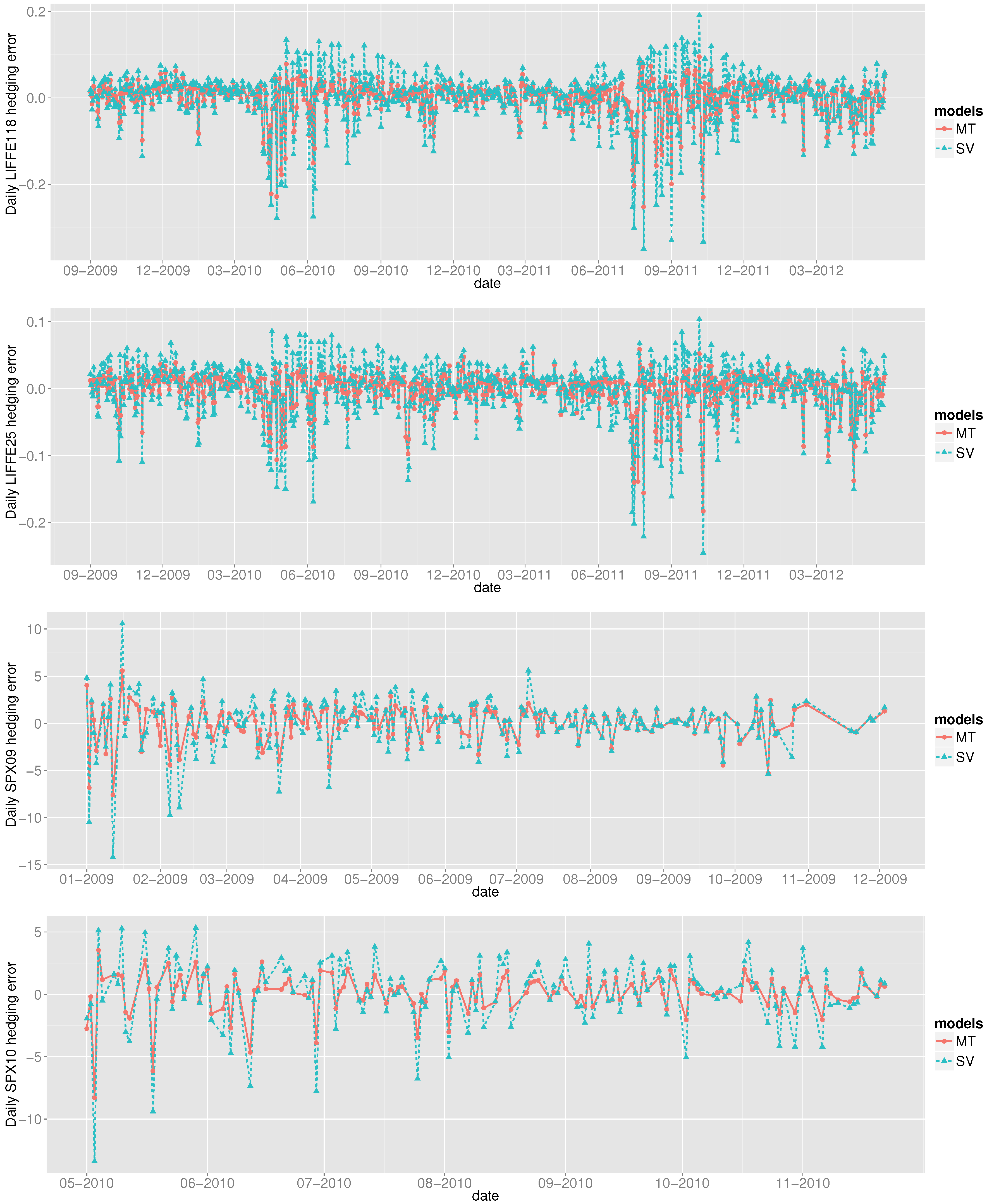
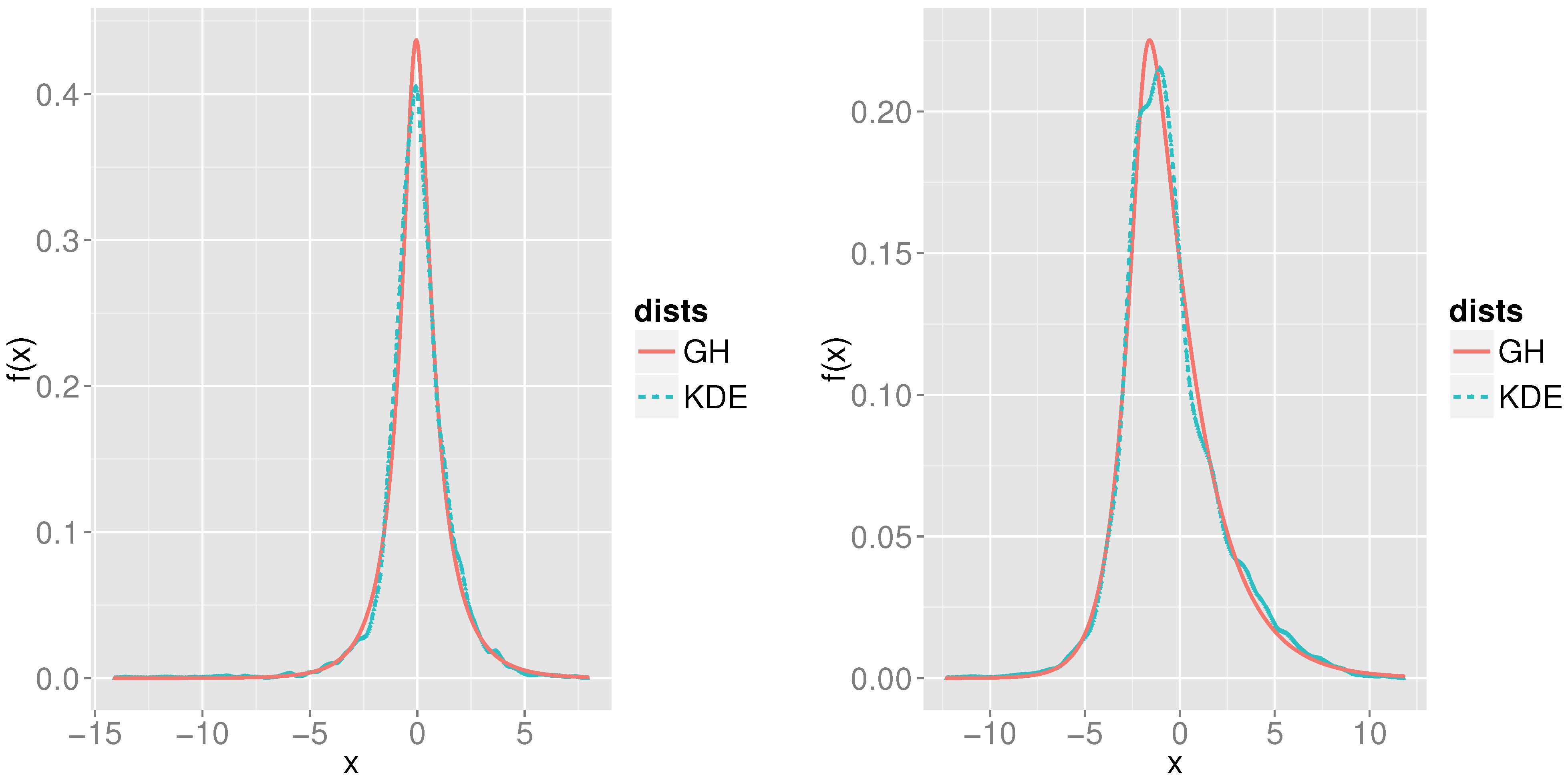
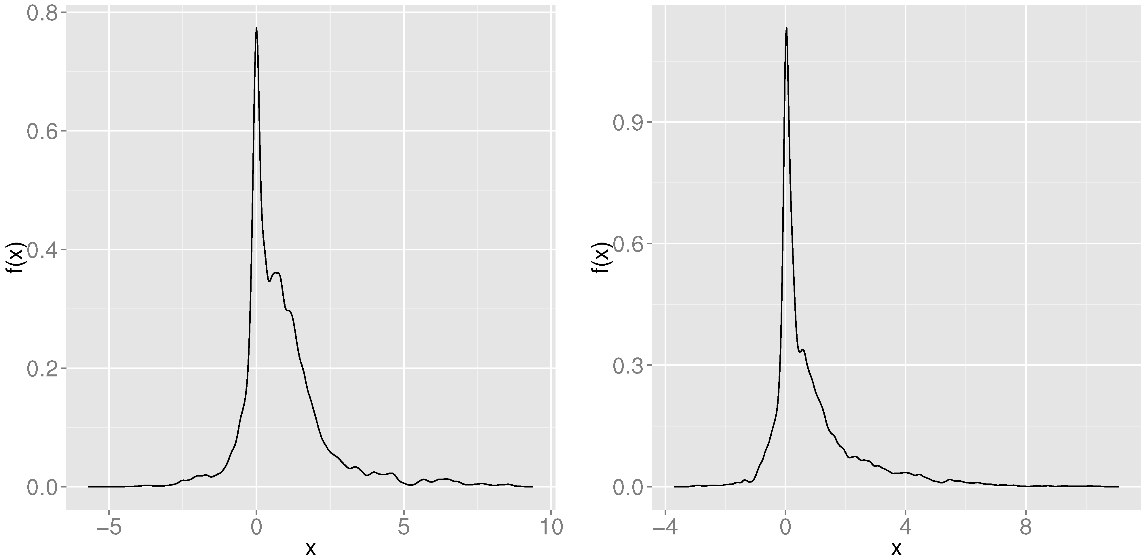