Forecasting Returns with Fundamentals-Removed Investor Sentiment

Abstract

The Baker and Wurgler (2006) sentiment index purports to measure irrational investor sentiment, while the University of Michigan Consumer Sentiment Index is designed to largely reflect fundamentals. Removing this fundamental component from the Baker and Wurgler index creates an index of investor sentiment that may better capture irrational sentiment. This new index predicts returns better than the original Baker and Wurgler index as well as the alternative Baker and Wurgler sentiment index.

1. Introduction

A common goal in studying investor sentiment is to find whether sentiment can explain returns. Or, do irrational investors cause mispricing that predictably reverses itself in the next period? The key to confirming this hypothesis is finding the right measure of irrational behavior, or investor sentiment. There are many different measures of investor sentiment in the literature, the most popular recently being Baker and Wurgler’s [1] index. As Baker and Wurgler [1] state, mispricing can occur when there are sufficient limits to arbitrage, and uninformed demand shocks occur. Therefore, the ideal sentiment measure would consist entirely of irrational (non-fundamental) investor behavior. Then, this pure measure of investor sentiment should have significant predictive power for future returns. This paper argues that the existing proxies of sentiment fall short in this regard.

The sentiment index used in Baker and Wurgler [1] may be the most complete measure in the current literature. They create a composite measure of investor sentiment using principal-components analysis. They use six components: closed-end fund discount, market turnover, number of IPOs, average first-day return of IPOs [2,3,4,5], gross equity share, and a dividend premium measure. However, if one wants a purer measure of sentiment that better captures mispricing, then their sentiment index should be altered. They create a principal-components index based on existing sentiment proxies in the literature, but there are likely to be some rational or fundamental components involved. In order to arrive at a better sentiment measure, the non-fundamental component should be separated from the fundamental components of the Baker and Wurgler index (BW hereafter). However, properly removing as much of the fundamental component as possible is tricky. Baker and Wurgler do attempt to do this by removing what they call business cycle variation from their sentiment measure. They regress each individual component against a dummy variable for NBER recessions, industrial production index growth, and growth in consumer durables, nondurables, and services, and then run principal-components on these six residuals. The sentiment index is still likely to contain rational reactions to fundamentals that do not move with the business cycle. This paper provides empirical confirmation that indeed the BW procedure may not fully remove fundamentals.

A measure of investor sentiment that fully removes fundamentals should do a superior job of forecasting returns due to the following: prices move away from fundamentals when noise trading is correlated and arbitrage is limited, and then deviations are eventually reversed. The basic hypothesis is that mispricing due to sentiment shows up in the aggregate so that market returns are predictable by a pure irrational sentiment measure. 1 This assumes that sentiment drives predictability of returns more than fundamentals, which admittedly may not have a strong prior. However, the evidence in this paper supports the idea of return predictability being due to sentiment and not fundamentals. If sentiment predicts returns only because it captures fundamental factors, then the new sentiment index created in this paper should perform worse in forecasting. However, the opposite is true. Thus, evidence in contrast with some of the literature in this area is provided. It should be noted, though, that Campbell and Kyle [6] find that mispricing can affect aggregate returns, and Lemmon and Portniaguina [7] mention that rational and behavioral hypotheses are not mutually exclusive.

It is also important here to note the difference between in-sample explanatory power and out-of-sample predictability. It is common for a model to perform well in sample but poor out-of-sample. As shown in Section 4, the BW index is more significant in sample than the Baker and Wurgler [1] index that removes business cycle variation. When moving out of sample, though, the BW index performs poorly. The new sentiment index is not intended to fully explain market returns. Rather, the intent is to capture deviations in expected return which are due to irrational mispricing (sentiment). An index that successfully does this should work better out of sample but not necessarily in sample.

This paper removes fundamentals from BW in a way similar to Lemmon and Portniaguina [7]. Lemmon and Portniaguina [7] use a set of fundamentals that is sufficiently different (and arguably more complete) from Baker and Wurgler’s [1] business cycle variables. Lemmon and Portniaguina [7] separate the fundamental and non-fundamental components of consumer confidence (CC hereafter). They use the non-fundamental component as a proxy for investor sentiment. This paper follows their methodology, but applies it to the Baker and Wurgler [1] index by first regressing CC on a set of fundamentals, then regressing BW on the fitted (fundamental/rational) value from this initial regression, and finally using the residuals from this regression as a proxy for pure sentiment.

Basically, the Lemmon and Portniaguina [7] measure of fundamental consumer confidence is removed from the Baker and Wurgler [1] index. Thus, a composite index of fundamentals based on consumer confidence is removed from Baker and Wurgler’s [1] composite index of sentiment. This composite index of fundamentals should limit any measurement errors or over-fitting of fundamentals when removing them from BW. 2 Also, Lemmon and Portniaguina’s [7] set of fundamentals (which this paper uses with some minor changes) is a more complete measure of overall fundamentals compared to Baker and Wurgler’s [1] business cycle variables. This paper shows that, empirically, following this methodology allows investor sentiment to forecast market returns better.

Instead of directly following Lemmon and Portniaguina [7], this paper uses BW for forecasting instead of CC, as it is a market measure of investor sentiment. 3 Market measures of sentiment are composed of real actions by investors directly involved in the market. For surveys (especially consumer confidence surveys), a participant may feel overly optimistic but may not actually act on this optimism. Surveys are also open to problems such as dishonesty, bias, and incomplete responses. A market measure of sentiment (such as BW) will match investors’ actions as it relates to their overall feeling of the stock market. Thus, this paper proposes that a market measure of investor sentiment will forecast market returns better than a survey-based measure. Empirical evidence is presented in support of this hypothesis, as the new index performs better in forecasting market returns than both Baker and Wurgler’s [1] index and their alternative sentiment index that removes business cycle variations (BWA hereafter).

To measure the predictive power of the new index, a linear forecasting model is used to forecast one-month-ahead market returns. The sample runs from July 1978, when the University of Michigan consumer sentiment survey became available in a monthly frequency, to December 2010. A simple investment strategy is used: if the one-month-ahead predicted excess market return is higher than the historical average of all previous months in the sample at the time of forecasting, then the investor will invest in the market. Otherwise, she invests in a risk-free asset (T-bills). Essentially, the goal is to time the market. This differs from both Baker and Wurgler [1] and Lemmon and Portniaguina [7], where no market timing is involved. Market timing is considered here for two reasons. First, it is a practical application of investor sentiment, in that it is usable by practitioners. Since a common goal in the sentiment literature is predicting returns, market timing is a natural extension. The second reason for using a market timing approach is that it provides economic significance (via realized returns) in addition to statistical significance. Following the investment strategy (essentially switching between stocks and bonds), the forecast model that removes the fundamental component of CC from BW provides average realized excess returns of around 10.6% annually compared to around 5.3% annually for BW and 8.0% annually for BWA. This new sentiment index also has significant market timing ability, as will be shown later. The excess market return average over the forecasting sample is around 6.7% annually (the return from a buy-and-hold strategy), so a forecast model utilizing only BW would not beat the market on average. This new index performs significantly better than both CC and Lemmon and Portniaguina’s [7] sentiment component of CC (by itself) as well. Since sentiment is typically thought to affect small, young, and volatile stocks the most, forecasting is also performed on a small-size portfolio. Again, removing the fundamental component increases the realized returns an investor could obtain. The evidence supports the hypothesis that investor sentiment should have no fundamental (rational) component, and that the existing measures of sentiment do not properly remove fundamentals. It should be noted that predictability in returns may be driven somewhat by time-varying risk and risk aversion, and not entirely by sentiment. However, this paper provides evidence that creating a better measure of irrationality increases predictability in returns.

The paper proceeds as follows: Section 2 reviews the existing literature on investor sentiment and consumer confidence as a proxy for sentiment; Section 3 discusses the data and methodology used; Section 4 discusses the results; and Section 5 concludes the paper.

2. Literature Review

DeLong et al. [8] show that returns of assets mostly held by noise traders can be predictable as mispricing caused by correlated sentiment (with limited arbitrage) will eventually correct itself. 4 Most studies (Baker and Wurgler [1], Lemmon and Portniaguina [7], etc.) show that small and young firms (and closed-end funds, discussed shortly) are predominantly held by noise traders and thus are more susceptible to sentiment. However, Campbell and Kyle [6] show that overreaction can impact aggregate stock values as well. Hence sentiment may also be able to predict market returns.

Lee, Shleifer, and Thaler [2] show that closed-end fund discounts may be due to investor sentiment. In their study, the returns of ten size-ranked portfolios are regressed against market returns and the change in a value-weighted closed-end fund discount variable. They find that the smallest size-ranked portfolio moves closely with closed-end funds, while the largest size-ranked portfolio moves in the opposite direction of closed-end funds.

The papers that follow Lee, Shleifer, and Thaler [2] are at the core of the field of investor sentiment. Barberis, Shleifer, and Vishny [10] present a model of investor sentiment that supports the findings that stock prices underreact to earnings announcements and overreact to successive good or bad news. Elton, Gruber, and Busse [11] show that changes in closed-end fund discounts do not explain common stock returns when including a value-weighted industry return index. They also find that investor sentiment is not a priced factor in common stocks as well as closed-end funds. Neal and Wheatley [3] find that closed-end fund discounts can predict the size premium, but nothing else.

Other authors have considered proxies or measures of investor sentiment outside of closed-end fund discounts. Lee, Jiang, and Indro [12] use a GARCH-mean model and the Investor’s Intelligence survey as their sentiment proxy to show that sentiment is a priced systematic risk. Lowry [4] shows that investor sentiment may impact IPO volume. Cai et al. [13], find that sentiment affects variation in straight debt IPO volume, and Derrien [5] shows that sentiment may play a role in the initial return of IPOs. Baker and Stein [14] create a model in which high market liquidity indicates that the market is dominated by irrational investors, creating a role for sentiment.

There is a wide range of literature in which consumer confidence indices are used to proxy for investor sentiment. Fisher and Statman [15] find that consumer confidence impacts individual investors’ sentiment, but not institutional investors’ sentiment. They also find that consumer confidence will rise significantly when stock returns (using many different indices) are high, and that consumer confidence may have some predictive power for returns. Schmeling [16] uses consumer confidence to try to predict returns for 18 different countries. He finds that consumer confidence has predictive power up to 6 months, but dies out after that. Also, some countries’ consumer confidence measure has no predictive power whatsoever.

Lemmon and Portniaguina [7] use consumer confidence as a proxy for investor sentiment. As mentioned earlier, Lemmon and Portniaguina [7] create a sentiment proxy from consumer confidence by removing nine quarterly fundamentals and their lags. They point out that the rational hypothesis and sentiment hypothesis are not mutually exclusive. Therefore, by removing fundamentals they create a sentiment index similar to what this paper creates: an index where mispricing could only be due to sentiment, so that prices will reverse and be predictable. They use a quarterly index of the University of Michigan Consumer Sentiment Index (CC). They mention that from 1978–2002 their sentiment component and the Baker and Wurgler [1] index have a very small correlation and that their index does not support Baker and Wurgler’s [1] findings mentioned below. They do not attempt to predict market returns as this paper does. The other key difference in this paper is that here their fundamental component of CC (using monthly data) is then removed from BW (a more direct market measure) to be used in market timing.

As discussed in the previous section, Baker and Wurgler [1] create a composite investor sentiment index using principal-component analysis. They use their index to run a predictive regression on various long-short portfolios. Their main findings are that small, young, and volatile firms have low returns for the following year when current sentiment is high. Baker and Wurgler [17] create a first-differenced series of their 2006 sentiment indices, whereby they first-difference the individual components and then run principal-components analysis. They use the change index to test for return co-movement with sentiment, while using their 2006 levels index to forecast returns. Their findings are that speculative, difficult-to-arbitrage stocks and stocks with high volatility are impacted greatly by sentiment. They also find that high sentiment leads to lower future market returns (overreaction). This paper builds on this finding, and attempts to forecast market returns.

3. Data and Methodology

The sample period used in this paper runs from July 1978 (when the Michigan Survey began to consistently use monthly frequencies) to December 2010, using monthly data. Market return is the value-weighted CRSP measure that includes dividends. 5 The risk-free rate used is the rate on 3-month Treasury bills, obtained from the St. Louis Federal Reserve (FRED) website [19]. Excess market return is the difference between these two. The University of Michigan Consumer Sentiment Index (CC, or consumer confidence) is also obtained from the FRED website [19]. The Baker and Wurgler [1] index and its alternative that removes business cycle variation, along with the individual components, are obtained from Jeffrey Wurgler’s website [20]. Table 1 shows the descriptive statistics for these variables. 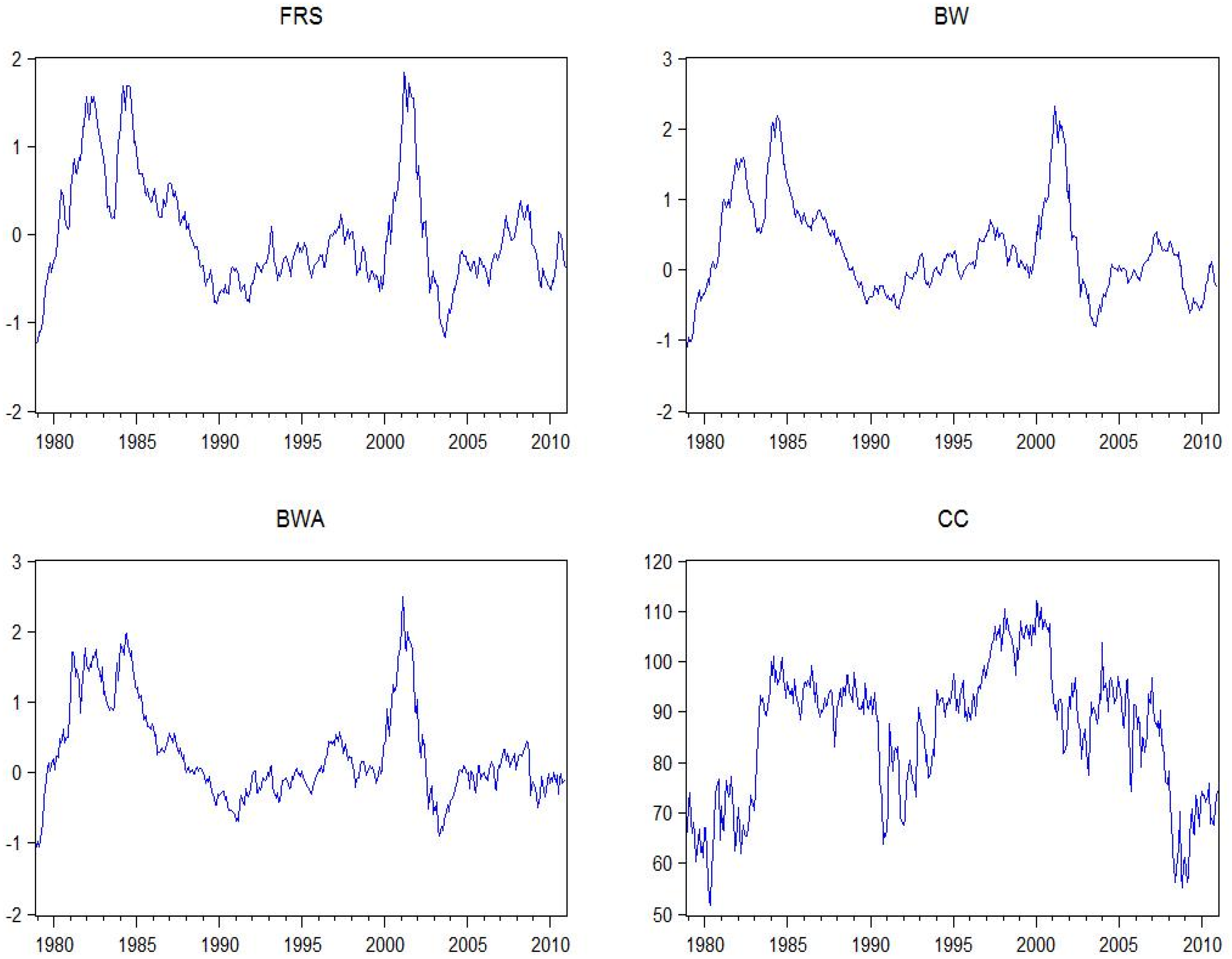Figure 1 provides time-series graphs of the excess market return, CC, BW, and BWA over the sample for comparison purposes.

Table 1. Descriptive Statistics.

Statistics	RF	MKTRET	CC	BW	BWA
Mean	0.004560	0.010268	86.18487	0.260882	0.245618
Median	0.004242	0.014399	90.2	0.1135	0.054
Maximum	0.013583	0.12967	112	2.321	2.497
Minimum	0.000025	−0.219503	51.7	−1.333	−1.273
Std. Dev.	0.002836	0.044035	13.18374	0.677739	0.68605
CV	0.621882	4.288566	0.152970	2.597876	2.793166
Skewness	0.666981	−0.778491	−0.436221	0.765964	0.861307
Kurtosis	0.465557	5.695326	2.408766	3.624503	3.405068

Sample: July 1978–December 2010, monthly intervals, giving 390 observations of each variable. CV is the coefficient of variation, which allows for comparison of CC and BW; RF is the risk-free rate in decimal form, as measured by the 3-month T-Bill, obtained from the FRED; MKTRET is the CRSP value-weighted portfolio; CC is the University of Michigan Consumer Sentiment Index; BW is the Baker-Wurgler investor sentiment index, from Baker & Wurgler [1], obtained from Jeffrey Wurgler’s website [20]; BWA is the Baker-Wurgler alternative index, which removes business cycle variation, from Baker & Wurgler [1].

Table 1. Descriptive Statistics.

Statistics	RF	MKTRET	CC	BW	BWA
Mean	0.004560	0.010268	86.18487	0.260882	0.245618
Median	0.004242	0.014399	90.2	0.1135	0.054
Maximum	0.013583	0.12967	112	2.321	2.497
Minimum	0.000025	−0.219503	51.7	−1.333	−1.273
Std. Dev.	0.002836	0.044035	13.18374	0.677739	0.68605
CV	0.621882	4.288566	0.152970	2.597876	2.793166
Skewness	0.666981	−0.778491	−0.436221	0.765964	0.861307
Kurtosis	0.465557	5.695326	2.408766	3.624503	3.405068

Sample: July 1978–December 2010, monthly intervals, giving 390 observations of each variable. CV is the coefficient of variation, which allows for comparison of CC and BW; RF is the risk-free rate in decimal form, as measured by the 3-month T-Bill, obtained from the FRED; MKTRET is the CRSP value-weighted portfolio; CC is the University of Michigan Consumer Sentiment Index; BW is the Baker-Wurgler investor sentiment index, from Baker & Wurgler [1], obtained from Jeffrey Wurgler’s website [20]; BWA is the Baker-Wurgler alternative index, which removes business cycle variation, from Baker & Wurgler [1].

As can be seen from Table 1, the average market return for the sample used here is about 12.3% annually (1.027% monthly). The average excess market return is slightly less than 7% annually. CC uses 1966 as its base year, with CC = 100. BW is from a standardized principal-component analysis, so that the series (although not necessarily in the sample used here) has a unit variance and a mean of zero. As described in the literature review, BW is comprised of six individual sentiment components and employs both leads and lags.

While CC is definitively non-stationary, BW’s stationarity is ambiguous using Dickey-Fuller, Dickey-Fuller GLS, and Phillips-Perron tests. For BW, the Dickey-Fuller GLS test shows that it is non-stationary, but the other tests are inconclusive. It appears that BW may be non-stationary due to the non-stationarity of just one component, the turnover component. Further, CC and BW may be cointegrated, using the Johansen integration test. The results are not definitive, as would be expected since BW may or may not be non-stationary.

Figure 1. This figure shows time-series graphs of the paper’s modified BW index (FRS), BW, BWA, and CC. FRS is fundamental-removed-sentiment, BW is Baker and Wurgler’s [1] sentiment index, BWA is Baker and Wurgler’s [1] sentiment index that removes business cycle variation, and CC is the University of Michigan Consumer Sentiment Index. Sample is from July 1978–December 2010.

Figure 1. This figure shows time-series graphs of the paper’s modified BW index (FRS), BW, BWA, and CC. FRS is fundamental-removed-sentiment, BW is Baker and Wurgler’s [1] sentiment index, BWA is Baker and Wurgler’s [1] sentiment index that removes business cycle variation, and CC is the University of Michigan Consumer Sentiment Index. Sample is from July 1978–December 2010.

Initially, Lemmon and Portniaguina’s [7] methodology is implemented, with some minor changes. Primarily, Lemmon and Portniaguina [7] use quarterly data and this paper uses monthly data. Lemmon and Portniaguina [7] use the following nine fundamentals: default spread (DEF), as measured by the difference between the yields to maturity on Moody’s Baa-rated bonds and Aaa-rated bonds; yield on 3-month Treasury bills (RF); dividend yield (DIV), following Fama and French [21]; real GDP growth (GDP); growth in personal consumption expenditures (CONS); labor income growth (LABOR), as measured by the per capita growth in total personal income minus dividend income, deflated by the PCE deflator; the Bureau of Labor Statistics unemployment rate (URATE), seasonally adjusted; inflation rate (INF), measured by the change in the consumer price index; and the consumption-to-wealth ratio (CAY) from Lettau and Ludvigson [22]. The dividend yield measure can be obtained from the difference between CRSP’s value-weighted return index and its value-weighted return index excluding dividends. The CAY measure is obtained from Martin Lettau’s website [23]. The seven other fundamental variables can be obtained from FRED’s website [19].

This paper makes two changes to Lemmon and Portniaguina’s [7] choice of fundamentals: instead of using the unemployment rate the prime rate on bank loans (PRIME) is used, and CAY and GDP are interpolated to monthly data. PRIME is obtained from FRED. The prime rate is essentially a benchmark for other loan rates, so it should broadly capture fundamental economic activity. Also, the unemployment rate is a survey measure, while the other fundamentals (and the prime rate) are directly observable. 6 The prime rate is more quickly accessible to investors than is the unemployment rate as well. Following Lemmon and Portniaguina [7], CC is regressed against these 9 fundamentals and their lags using monthly data. Since Lemmon and Portniaguina [7] use quarterly indices with one lead and one lag (giving six months of data), the lead on each fundamental along with 5 monthly lags is used. Since CAY and GDP are converted to monthly, only a lead and one 3-month lag can be used for these two variables to avoid multicollinearity. This gives the following:

$$C{C}_t={\text{α}}_0+{\displaystyle \sum _{i=0}^5\left[{\text{α}}_i\right]*[X_{t-i}]}+v_t=CCfi{t}_t+v_t$$

(1)

${\text{α}}_0$ is a constant, $[{\text{α}}_i]$ is a vector of coefficients: $[X]=[DEF,RF,DIV,CONS,INF,LABOR,PRIME,CAY,GDP]\prime$, $CCfi{t}_t$ is the fitted value of the regression, and $v_t$ is the error term (noting that CAY and GDP only have one lag at t − 3).

The fitted value from the above equation is obtained by multiplying the coefficient by the respective value for that variable (from i = 0 to 5) and summing them together with the intercept for each particular month. This produces the “fundamental” or “rational” component of CC, whereas the residual is the sentiment component as in Lemmon and Portniaguina [7]. As discussed in the introduction, the idea is to weight the fundamentals on the non-market survey measure of consumer confidence before removing it from BW. The aim is to remove the rational, fundamental component of BW, leaving only irrational investor sentiment (which produces market mispricing). 7

Each regression is rolled forward one month, while anchoring the starting point. This is done so that only information from time 1 to t is utilized in forecasting at month t + 1. Therefore, the coefficients will change as the regression updates forward each month in a stepwise fashion. The fitted values of Equation (1) are saved each time so that a series is created to be used in forecasting. That is, Equation (1) is run from time 1 to time t, with t fitted values created. This series can be used to then forecast at t + 1, as will be explained later. To forecast the next month (t + 2), Equation (1) is then run from time 1 to t + 1, creating t + 1 values in each series. Thus, Equation (1) is updated each month as forecasting moves from the halfway point to the last period in the sample. When running Equation (1) for the entire sample, the adjusted R-squared value is 0.78, which is very close to the value that Lemmon and Portniaguina [7] obtain.

The fitted (fundamental) CC values are then used to properly remove fundamentals from BW. Again, BW is used to forecast as it is a market-based measure and should forecast market returns better. Lemmon and Portniaguina’s [7] methodology has been used up to this point in order to get a proper measure of fundamentals. Now, after obtaining the series of fitted values from Equation (1), the following is run:

$$B{W}_t=a+b*CCfi{t}_t+e_t$$

(2)

$$e_t\equiv FR{S}_t$$

(3)

CCfit is the fitted value of CC from Equation (1). The procedure in Equation (2) is the same as in Equation (1). The residual from Equation (2), $e_t$, is hereafter referred to as FRS (fundamental-removed sentiment). Note that using only CCfit eliminates any endogeneity issues that would arise from using CC in Equation (2). The reason is that since CC also has a sentiment component, it would be correlated with the residual from Equation (2), or FRS. 8 CCfit is used as a composite index of fundamentals which should help prevent potential over-fitting or measurement errors when removing fundamentals from sentiment. Table 2 shows the descriptive statistics for FRS, when forecasting starts at the one-third mark of the sample as will be done later. Note that this is the series of only time t residual from Equation (2), where time t is used to forecast excess market return at time t + 1. Since FRS contains residuals from different regressions, it is not necessarily expected that its mean be zero (as opposed to a series of residuals from one regression). It should also be noted that FRS is unambiguously stationary when BW is modified using this methodology. As discussed at the beginning of this section, BW is found to be non-stationary using some statistical tests.

Table 2. FRS Descriptive Statistics.

Statistics	FRS
Mean	−0.319224
Median	−0.398
Maximum	1.815
Minimum	−1.254
Std. Dev.	0.53787
Skewness	1.452870
Kurtosis	6.435207

Sample is from April 1989 to November 2010. Thus, when forecasting is performed starting at the one-third mark of the full sample, excess market return is forecasted starting at May 1989 up until December 2010, at one-month intervals. FRS (fundamental-removed sentiment) is the series of residuals from Equation (2), where only the final residual of each recursive regression is saved. This produces the time t residual, e, which is used in forecasting the market at t + 1.

Table 2. FRS Descriptive Statistics.

Statistics	FRS
Mean	−0.319224
Median	−0.398
Maximum	1.815
Minimum	−1.254
Std. Dev.	0.53787
Skewness	1.452870
Kurtosis	6.435207

Sample is from April 1989 to November 2010. Thus, when forecasting is performed starting at the one-third mark of the full sample, excess market return is forecasted starting at May 1989 up until December 2010, at one-month intervals. FRS (fundamental-removed sentiment) is the series of residuals from Equation (2), where only the final residual of each recursive regression is saved. This produces the time t residual, e, which is used in forecasting the market at t + 1.

The regression in Equation (2) is run in a stepwise fashion with an anchored starting point, with the end point starting from the halfway point (October 1994) updating each time to include the next month. Equation (2) can be thought of as running simultaneously with Equation (1). The residuals from Equation (2) are then used in forecasting excess market returns, with each month in which forecasting is done having its own unique series of the residuals from Equation (2) that does not include any future information. The R-squared value from Equation (2) is 8% for the full sample, although it ranges from 3%–8% over the sample.

The following forecasting models are employed:

$$\text{Model i}:{\widehat{R}}_t={\text{α}}_t+{\text{β}}_t*sen{t}_{t-1}^i+{\text{η}}_t \text{i}=\text{1},\text{2},\text{3}$$

(4)

${\widehat{R}}_t$ is the predicted excess market return and $sen{t}_{t-1}^i$ is the appropriate sentiment measure, lagged one month, for model i. For Model I (i = 1) BW is used for “sent”, for Model II (i = 2) BWA is used, and for Model III (i = 3) FRS is used. BWA is included for comparison purposes; this also shows that BW removes some fundamentals but ultimately falls short. Forecasting is done from October 1994 to December 2010 and also from May 1989 to December 2010. Therefore, out-of-sample forecasts for the second half of the sample are obtained, and also for the last two-thirds of the sample for comparison and robustness. So when forecasting starts at the halfway point of the sample, the forecasting equations above start by running from July 1978–September 1994, and finish by running from July 1978–November 2010. Ordinary least squares is used in the forecasting equations, and one-month-ahead forecasts of the excess market returns, ${\widehat{R}}_t$, are obtained using the residuals of the forecasting equations.

4. Results

4.1. Forecast Results

Table 3 shows the results from the forecasting regressions for each of the three models (for the first case when forecasting starts at the halfway point of the sample). The coefficients, t-statistics (reported in parentheses), and R-squared values in the table are averages from the 195 individual forecasting regressions for each model, with each regression adding one additional data point. T-statistics are obtained by following the Fama-MacBeth [24] methodology, using the distribution of the 195 coefficients. Note that these t-statistics should not be biased since the standard two-pass approach with generated regressors is not used here. Excess market returns are the dependent variables in each model and its respective regressions. Coefficients for each variable are small, but the coefficients are difficult to interpret in terms of size due to how CC and BW are created, as well as the fact that residuals from Equation (2) are used as independent variables.

In-sample R-squared values are low for each model, as is common in return forecasting. Campbell and Thompson [25] provide a way to examine whether a model provides sufficient explanatory power. Using out-of-sample (OOS) R-squared values based on the historical mean, the OOS R-squared value can be compared to the squared Sharpe ratio (here of the excess market return) over the forecasting sample. When the time interval is small (monthly is small enough) then a mean-variance investor can use Model III (FRS) to increase her monthly expected portfolio return by a proportional factor of $R^2$/$S{R}^2$ (out-of-sample R-squared over the squared Sharpe ratio for the forecasting sample). Here, Model III gives 1.3/1.5 = 86% proportional increase in expected return from observing FRS.

Model III, when removing CCfit from BW and using this residual to forecast excess market returns (FRS), is the most significant, with the most negative coefficient. FRS is a measure of uninformed demand shocks, which cause mispricing and subsequent reversal. A one standard deviation increase in FRS for this particular subsample implies a 0.25% decrease in next month’s excess market return. Thus, sentiment and excess market returns have a negative relationship. This can be interpreted as overreaction on the part of investors.

Table 3. Forecast Regression Results.

EMR:	Model I	Model II	Model III
BW
Coefficient	−0.0036
T-stat	(−1.91) *
BWA
Coefficient		−0.0037
T-stat		(−1.73) *
FRS
Coefficient			−0.0040
T-stat			(−2.00) *
R-Squared	0.0041	0.0046	0.0044

* denotes significance at the 10% level. The table shows the average of coefficients from forecasting equations for various forecast models, with monthly market returns as the dependent variable. T-statistics are created using the Fama-MacBeth [24] methodology. Forecasting starts at the halfway point of the sample (October 1994), rolling forward each month, creating 195 forecasting equations. Note that constants are not reported here. Model I uses the Baker-Wurgler index to forecast excess market returns, Model II uses the orthogonal Baker-Wurgler index that removes business-cycle variation to forecast, and Model III uses the new FRS (fundamental-removed sentiment) index from Equations (1)–(3). Sample: July 1978–December 2010, monthly intervals.

Table 3. Forecast Regression Results.

EMR:	Model I	Model II	Model III
BW
Coefficient	−0.0036
T-stat	(−1.91) *
BWA
Coefficient		−0.0037
T-stat		(−1.73) *
FRS
Coefficient			−0.0040
T-stat			(−2.00) *
R-Squared	0.0041	0.0046	0.0044

* denotes significance at the 10% level. The table shows the average of coefficients from forecasting equations for various forecast models, with monthly market returns as the dependent variable. T-statistics are created using the Fama-MacBeth [24] methodology. Forecasting starts at the halfway point of the sample (October 1994), rolling forward each month, creating 195 forecasting equations. Note that constants are not reported here. Model I uses the Baker-Wurgler index to forecast excess market returns, Model II uses the orthogonal Baker-Wurgler index that removes business-cycle variation to forecast, and Model III uses the new FRS (fundamental-removed sentiment) index from Equations (1)–(3). Sample: July 1978–December 2010, monthly intervals.

Table 4 shows the forecast results. To measure forecast (market timing) accuracy, a simple investment strategy is implemented. The one-month-ahead forecast of excess market return is compared to the historical average of the excess market return. So if the predicted value of the excess market return ($\widehat{R}$) is calculated at time t + 1, the relevant historical average of the excess market return is calculated from time 1 to t. If ${\widehat{R}}_{t+1}$ is higher than the average obtained from existing data at that point (at time t), then the investor will invest only in the market in the following month (t + 1), obtaining the actual market return in that period. However, if ${\widehat{R}}_{t+1}$ is less than the historical average, then the investor will invest only in the risk-free asset in the following month, obtaining the actual risk-free return. This produces a time series of realized investment returns for each forecasting model. That is what this paper is concerned with; it produces a measure of the ability of each model to time the market. This is also the return an investor could conceivably have earned when using the respective model to forecast based on the investment rule, since out-of-sample forecasting is done. Panel A of Table 4 provides for each model the realized investment excess return, standard deviation, and risk-corrected average realized investment returns. Note that realized investment returns are either market returns or risk-free returns (minus the risk-free rate). Returns reported in Table 4 are annualized monthly returns.

Table 4. Forecasting results.

Panel A: Realized Returns
Time Series Statistics	Model I	Model II	Model III	Model III − Model I	Model III − Model II
Realized investment excess returns (average)	5.297%	7.978% **	10.643% ***	5.376% **	2.665% *
Realized investment excess returns (median)	1.807%	1.876%	9.394% ***	7.587% ***	7.518% ***
Realized returns after removing top 1% (average)	4.137%	6.846% **	9.539% ***	5.402% **	2.693% *
Standard deviation of realized returns	3.536%	3.216%	3.805%
Realized returns after market risk correction	1.718%	4.967% ***	6.400% ***	4.682% **	1.433%
Realized returns after FF3 correction	2.283%	4.418% **	5.846% ***	3.563% *	1.428%
Realized returns after FF3 and momentum correction	1.571%	4.091% **	5.371% ***	3.800% *	1.280%
Panel B: Market Timing Ability Tests for Model III
Independent Variable	TM	HM	CM
α	0.0002 (0.002)	−0.0043 (0.003)	−0.0172 (0.009) *
R	0.7104 (0.087) ***	0.9244 (0.095) ***
R2	2.0954 (1.010) *
D		0.4676 (0.221) **
I			0.0283 (0.009) ***

Panel A shows the average annualized realized returns for the various models. Excess market returns use value-weighted CRSP market returns and 3-month T-bill rates for the risk-free rate. Realized investment returns are based off an investment strategy of investing in the market if predicted returns are higher than a stepwise average of excess market returns for all previous months or investing in the risk-free asset if predicted returns are lower than this average. Realized returns are from October 1994–December 2010. The third row shows the average returns when removing the top 1% of realized returns obtained. The realized returns are corrected for risk using a simple beta formulation, Fama and French [26] 3-factor model, and Carhatt [27] 4-factor model. In Columns 2–4, * represents significance at ten percent, ** at 5%, and *** at 1% using 20,000 simulations where the market and risk-free asset are randomly picked each month using the same ex-post weight of the corresponding model. See Section 4.3 for more details. Columns 5 and 6 in Panel A show the difference in returns between Models III and I, and Models III and II, respectively. The significance levels here are obtained from a bootstrapping procedure, using the sample of 195 return observations and 10,000 simulations. The null hypothesis is that the two series have a difference of zero. Panel B shows the market timing test results for Model III over the same sample period as Panel A. TM is the Treynor and Mazuy [28] test, HM is the Henriksson and Merton [29] test, and CM is the Cumby and Modest [30] test. α is the intercept, R is the CRSP value-weighted excess market return, D is the dummy variable from Henriksson and Merton [29]: D = max [0, rf − r] (where rf is the return on 3-month U.S. Treasury bills), r is the excess market return, and I is the Cumby and Modest [30] dummy variable: I = 1 if the model predicts a return higher than average and I = 0 otherwise. The Cumby and Modest [30] test uses the excess market returns as the dependent variable. Coefficients for each variable are provided, along with the Newey-West [31] standard errors in parentheses, with 2 lags based on Akaike Information criterion. * represents significance at the 10% level, ** significance at the 5% level, and *** significance at the 1% level.

Table 4. Forecasting results.

Panel A: Realized Returns
Time Series Statistics	Model I	Model II	Model III	Model III − Model I	Model III − Model II
Realized investment excess returns (average)	5.297%	7.978% **	10.643% ***	5.376% **	2.665% *
Realized investment excess returns (median)	1.807%	1.876%	9.394% ***	7.587% ***	7.518% ***
Realized returns after removing top 1% (average)	4.137%	6.846% **	9.539% ***	5.402% **	2.693% *
Standard deviation of realized returns	3.536%	3.216%	3.805%
Realized returns after market risk correction	1.718%	4.967% ***	6.400% ***	4.682% **	1.433%
Realized returns after FF3 correction	2.283%	4.418% **	5.846% ***	3.563% *	1.428%
Realized returns after FF3 and momentum correction	1.571%	4.091% **	5.371% ***	3.800% *	1.280%
Panel B: Market Timing Ability Tests for Model III
Independent Variable	TM	HM	CM
α	0.0002 (0.002)	−0.0043 (0.003)	−0.0172 (0.009) *
R	0.7104 (0.087) ***	0.9244 (0.095) ***
R2	2.0954 (1.010) *
D		0.4676 (0.221) **
I			0.0283 (0.009) ***

Panel A shows the average annualized realized returns for the various models. Excess market returns use value-weighted CRSP market returns and 3-month T-bill rates for the risk-free rate. Realized investment returns are based off an investment strategy of investing in the market if predicted returns are higher than a stepwise average of excess market returns for all previous months or investing in the risk-free asset if predicted returns are lower than this average. Realized returns are from October 1994–December 2010. The third row shows the average returns when removing the top 1% of realized returns obtained. The realized returns are corrected for risk using a simple beta formulation, Fama and French [26] 3-factor model, and Carhatt [27] 4-factor model. In Columns 2–4, * represents significance at ten percent, ** at 5%, and *** at 1% using 20,000 simulations where the market and risk-free asset are randomly picked each month using the same ex-post weight of the corresponding model. See Section 4.3 for more details. Columns 5 and 6 in Panel A show the difference in returns between Models III and I, and Models III and II, respectively. The significance levels here are obtained from a bootstrapping procedure, using the sample of 195 return observations and 10,000 simulations. The null hypothesis is that the two series have a difference of zero. Panel B shows the market timing test results for Model III over the same sample period as Panel A. TM is the Treynor and Mazuy [28] test, HM is the Henriksson and Merton [29] test, and CM is the Cumby and Modest [30] test. α is the intercept, R is the CRSP value-weighted excess market return, D is the dummy variable from Henriksson and Merton [29]: D = max [0, rf − r] (where rf is the return on 3-month U.S. Treasury bills), r is the excess market return, and I is the Cumby and Modest [30] dummy variable: I = 1 if the model predicts a return higher than average and I = 0 otherwise. The Cumby and Modest [30] test uses the excess market returns as the dependent variable. Coefficients for each variable are provided, along with the Newey-West [31] standard errors in parentheses, with 2 lags based on Akaike Information criterion. * represents significance at the 10% level, ** significance at the 5% level, and *** significance at the 1% level.

From the table it can be seen that using the Baker-Wurgler [1] index to forecast (Model I) provides average realized investment excess returns of about 5.3% annually (8.6% prior to subtracting the risk-free rate), and a realized standard deviation of about 3.5% (Sharpe ratio of 1.50). The alternative Baker and Wurgler [1] index that removes business cycle variation (Model II) provides average excess returns of 8.0% (11.3%) and a standard deviation of 3.2% (SR = 2.48). However, one can do even better when removing the fundamental component of CC from BW (Model III, using FRS), with an average annual excess return of about 10.6% (13.9%) and a standard deviation of 3.8% (SR = 2.80). Model I does not beat the average market excess return for the forecasting sample period, which is around 6.7% annually. Note that this 6.7% would be the realized excess return from a buy-and-hold the market strategy, and the strategy would have a standard deviation of 4.8% (SR = 2.05). Model II beats a buy-and-hold strategy by 1.3%, and Model III beats a buy-and-hold by 3.9% for this sample. As mentioned previously, it is possible that returns are predictable in part due to time-varying risk and risk aversion and not solely due to investor sentiment, though performance increases as more fundamentals are removed. The results are even more divergent when using the median rather than the mean of realized returns, which is shown in the second row of Panel A. Models I and II drop to a 1.8% realized return, while Model III has a median of 9.4%. Models I and II produce realized returns that are skewed (more negative returns compared to Model III). In order to check if the positive results of Model III are due to a few outstanding months’ returns, the top 1% is dropped and the average of the remaining 99% is reported in the third row of Panel A. While the returns in Row 3 drop across the board (as to be expected), they still remain significantly positive at 1% for Model III.

Pesaran and Timmermann [32] raise the issue that a market timing portfolio that switches between stocks and bonds may have a lower standard deviation simply due to including bonds with low standard deviation. To address this, they construct a portfolio that randomly switches between stocks and bonds at the same proportion as their switching portfolio. The expected excess return of this portfolio with the CRSP market data and T-bills used in this paper would be 5.2% with a standard deviation of about 5.0%. Note that Model III provides a superior mean-variance tradeoff.

Also, BW does even worse in comparison after correcting for market risk, with an average annual return of about 1.7%. FRS gives market-risk-corrected returns of about 6.4% annually. BWA gives market-risk-corrected returns of about 5.0%, again falling below Model III but well above Model I (BW). The results stand after correcting for Fama and French’s [26] HML and SMB factors, and Carhart’s [27] momentum factor as well. The size factor has been suggested as possibly explaining abnormal returns from a sentiment-based trading strategy, but these results show otherwise. Model III (FRS) still provides an average annual return of 5.8% after correcting for market, size, and value. Momentum also does not fully explain the performance of FRS.

The last two columns of the table show the difference in returns between Model III and the other two models (or the improvement of FRS over BW and BWA). Significance levels are also shown, which are obtained from a bootstrapping procedure with 10,000 simulations. FRS offers an improved return at a 5% significance level over BW and at a 10% significance level over BWA. This is the case for both average returns and returns with the top 1% removed. For median returns, FRS offers an improvement at a 1% significance level over both BW and BWA. FRS offers a significant improvement over BW when using risk-adjusted returns. While the risk-adjusted returns of FRS are not a significant improvement over BWA using the bootstrapping procedure, there are two important points to consider. The first is that these returns are less volatile with a smaller range for all three models. Therefore, significance is more difficult to achieve. The second point is that the difference in risk-corrected returns between Models III and II are still economically substantial, with the difference in being between 1.2% and 1.4% per annum (note that this is essentially the alpha obtained).

4.2. Market Timing Tests

Looking at the realized returns that each model would provide for an investor provides a test of economic significance, but the market timing literature provides additional statistical tests for market timing ability. Three such tests are performed here for Model III over the October 1994–December 2010 forecasting sample, and the results can be seen in Panel B of Table 4. The first is the Treynor and Mazuy [28] test (TM hereafter), where a quadratic specification is implemented. The TM test for market timing ability is testing the null hypothesis that the coefficient on the squared excess market return is not positive, when the realized excess returns are regressed on a constant, the excess market return, and the squared excess market return. From Panel B it can be seen that Model III (FRS) has a large positive coefficient on the squared excess market return, and it is significant at 10% based on Newey-West [31] standard errors. Thus, there is significant market timing ability based on the TM test. 9

Henriksson and Merton [29] argue that market timers have different target betas depending on whether they predict an up or down market, therefore their test (the HM test) replaces the squared excess market return variable of the TM test with the following dummy variable:

$$D_t=\max [0,(r{f}_t-R_t)]$$

(5)

rf is the return on 3-month U.S. Treasury bills, and R is the excess market return. Panel B shows that the coefficient (timing ability) on this dummy variable is positive and significant at 5%. While the intercept in this specification can be interpreted as selection ability, Goetzman, Ingersoll, and Ivković [33] note that the selection ability coefficients and market timing ability coefficients are typically of the opposite sign.

The Cumby and Modest [30] test (CM), but following Breen, Glosten, and Jagannathan [34] is also performed. They do not assume a CAPM structure and directly test whether the expected realized return is different when an up market is predicted compared to when a down market is predicted. The dummy variable for this test (the variable I in Panel B of Table 4) is equal to one if the predicted return of Model III is higher than average, and equal to zero if it is less than average. Here, the excess market return is the dependent variable. Again, the market timing ability coefficient is positive and significant at 1%, providing positive evidence of timing ability. Breen, Glosten, and Jagannathan [34] also note that a negative intercept is equivalent to the expected return of the timing portfolio being higher than the return on the market (buy-and-hold strategy). Panel B shows a negative intercept that is significant at 10%.

In order to truly examine the potential profitability of the model, transaction costs must be taken into account. However, the emergence of ETFs has allowed for low transaction costs when switching between a market proxy portfolio (ETF) and a bond (possibly an ETF as well). For example, Vanguard advertises a 0.15% average ETF expense ratio, although it notes that the industry average according to Lipper, Inc. is 0.58% as of 31 December 2012. Vanguard’s CRSP total stock market index has an expense ratio of only 0.05%, but other mutual funds may be as high as 0.89% [35]. Table 5 shows the realized returns of each model after accounting for transaction costs. The high and medium numbers come from Pesaran and Timmermann [32]. They use a cost of 1% and 0.5% for the high and medium, respectively, transaction costs of stocks. These are close to the industry average of 0.58% and the upper end of mutual funds of 0.89%. Also, a low cost of 0.15% is given (Vanguard’s cost). A cost of 0.1% is used for bonds in all cases, as in Pesaran and Timmermann [32]. The costs are applied to stocks and bonds for each month in which the investor would hold the market (stocks) or the risk-free asset (bonds). From examining Table 4 it can be seen that the realized returns are not significantly lowered after accounting for transaction costs. 10

Table 5. Realized returns after transaction costs.

Transaction Costs	High	Medium	Low
Model I	5.243%	5.268%	5.286%
Model II	7.901%	7.937%	7.963%
Model III	10.529%	10.585%	10.624%

This table shows the average realized excess returns for each forecast model. Model I uses the Baker-Wurgler [1] index (BW), Model II uses the alternate Baker-Wurgler [1] index that removes business cycle variation (BWA), and Model III uses fundamental-removed sentiment (FRS) to forecast. High transaction costs are 1% for stocks and 0.1% for bonds; medium costs are 0.5% for stocks and 0.1% for bonds; low costs are 0.15% for stocks and 0.1% for bonds. Transaction costs are subtracted from monthly returns depending on whether stocks (market) or bonds (risk-free asset/T-bills) are chosen for that particular month. For example, if stocks are chosen in month t, then the transaction-cost-adjusted return for t is r(t) × (1 − c), where r is the return and c is the appropriate cost for stocks. Similar analysis is done for bonds, then an average of the full sample (October 1994–December 2010) adjusted returns is reported.

Table 5. Realized returns after transaction costs.

Transaction Costs	High	Medium	Low
Model I	5.243%	5.268%	5.286%
Model II	7.901%	7.937%	7.963%
Model III	10.529%	10.585%	10.624%

This table shows the average realized excess returns for each forecast model. Model I uses the Baker-Wurgler [1] index (BW), Model II uses the alternate Baker-Wurgler [1] index that removes business cycle variation (BWA), and Model III uses fundamental-removed sentiment (FRS) to forecast. High transaction costs are 1% for stocks and 0.1% for bonds; medium costs are 0.5% for stocks and 0.1% for bonds; low costs are 0.15% for stocks and 0.1% for bonds. Transaction costs are subtracted from monthly returns depending on whether stocks (market) or bonds (risk-free asset/T-bills) are chosen for that particular month. For example, if stocks are chosen in month t, then the transaction-cost-adjusted return for t is r(t) × (1 − c), where r is the return and c is the appropriate cost for stocks. Similar analysis is done for bonds, then an average of the full sample (October 1994–December 2010) adjusted returns is reported.

Several other forecast models are examined to provide a comparison. The results can be found in the Appendix. 11 None of the models examined come close to the performance of FRS. Interestingly, directly removing the fundamentals in Equation (1) from BW does poorly as well. Thus it appears that the CC index properly weights these fundamentals, which when removed from BW provide a better irrational measure of sentiment that also forecasts better. 12

4.3. Statistical Significance

In order to obtain a general idea of how well the investment strategies perform, the results from Model III are compared to random strategies that pick between the market and the risk-free asset randomly each month. A simulation is conducted where the market is picked about 80% of the time, as is the case with Model III. 13 Under the null hypothesis that excess market returns are not predictable (efficient market hypothesis), this would give an accurate distribution. Thus, our null hypothesis is the rational efficient market hypothesis, and our alternative hypothesis is the behavioral hypothesis (mispricing caused by noise trading). This analysis can also be seen as comparing the appropriate forecasting model to a random walk model. When performing the random draws 20,000 times, the percentage of times that the realized investment return beats Model III is indistinguishable from zero. In fact, only 14 out of 20,000 simulations beat Model III. This could be interpreted as a p-value of zero under the null hypothesis. Hence, the realized return of Model III would be significant at 1%, as shown in Table 4. For this model, the 1% cutoff is 9.0% average annual excess return, and for the 5% level it is 7.9% (compared to Model III’s performance of 10.6%). Following the same methodology (while changing the probability that the market is selected to match the appropriate model being used for comparison), Model II is beaten 2.8% of the time (significant at 5%) and Model I is beaten 24% of the time (insignificant). The same is done for risk-corrected returns, and those significance levels are denoted in Table 4 as well.

4.4. Robustness

Forecasting is also performed starting at the one-third mark of the sample (May 1989). This provides 260 months of forecasting one-month-ahead excess market returns, instead of the 195 produced earlier. Table 6 shows that the overall forecast results for the full forecasting sample (which is now two-thirds of the entire sample) are qualitatively the same as in Table 4. Again, removing the fundamental component of CC from BW provides the highest realized excess returns (Model III is again superior). In this longer sample period, the performance of BW/Model I can be completely explained by the known risk factors, while the performance of FRS is still significantly positive after risk correction. This is further support that Model III provides superior forecasting performance and realized investment returns. A buy-and-hold the market strategy would have provided a realized excess return of about 6.5% (standard deviation of 3.2%), so again Model I does not beat the market, while Model II is on par with the market. Model III again clearly outperforms the market. Model III again is clearly superior to the other two models when examining the median of realized returns rather than the mean. Also, the results are not due to a few positive outliers, as can be seen from the third row of the table, which drops the top 1% of realized returns and then takes the mean.

Table 6. Forecasting results for larger sample.

May 1989–December 2010 Forecasting Sample
Time Series Statistics	Model I	Model II	Model III	Model III − Model I	Model III − Model II
Realized investment excess returns	5.192%	6.571% *	9.505% ***	4.313% **	2.934% **
Realized investment excess returns (median)	1.429%	2.039%	9.310% ***	7.881% ***	7.271% ***
Realized returns after removing top 1% (average)	3.860%	5.255% *	8.223% **	4.363% **	2.968% **
Standard deviation of realized returns	3.513%	3.182%	3.745%
Realized returns after risk correction	1.279%	3.320% **	4.978% ***	3.699% **	1.658%
Realized returns after FF3 correction	0.117%	2.415% *	4.549% ***	4.432% ***	2.134% *
Realized returns after FF3 and momentum correction	−0.012%	2.083%	3.938% ***	3.950% **	1.855%

The above returns are annualized monthly returns. Excess market returns use the CRSP value-weighted average for market returns and the 3-month T-bill rate for the risk-free rate. Realized investment returns are based off investment strategy of investing in the market if predicted returns are higher than a stepwise average of excess market returns for all previous months or investing in the risk-free asset if predicted returns are lower than this average. Realized returns are from May 1989–December 2010. These realized returns are corrected for risk using a simple beta formulation, Fama and French [26] 3-factor model, and Carhatt [27] 4-factor model. Model I uses the Baker-Wurgler [1] index to forecast excess market returns, Model II uses the orthogonal Baker-Wurgler [1] index that removes business-cycle variation to forecast, and Model III uses the new fundamental-removed sentiment (FRS) index from Equations (1)–(3). In Columns 2–4, * represents significance at ten percent, ** at 5%, and *** at 1% using 20,000 simulations where the market and risk-free asset are randomly picked each month using the same ex-post weight of the corresponding model. Again, the null hypothesis is that returns are not predictable. See Section 4.3 and Section 4.4 for more details. Columns 5 and 6 show the difference in returns between Models III and I, and Models III and II, respectively. The significance levels here are obtained from a bootstrapping procedure, using the sample of 260 return observations and 10,000 simulations.

Table 6. Forecasting results for larger sample.

May 1989–December 2010 Forecasting Sample
Time Series Statistics	Model I	Model II	Model III	Model III − Model I	Model III − Model II
Realized investment excess returns	5.192%	6.571% *	9.505% ***	4.313% **	2.934% **
Realized investment excess returns (median)	1.429%	2.039%	9.310% ***	7.881% ***	7.271% ***
Realized returns after removing top 1% (average)	3.860%	5.255% *	8.223% **	4.363% **	2.968% **
Standard deviation of realized returns	3.513%	3.182%	3.745%
Realized returns after risk correction	1.279%	3.320% **	4.978% ***	3.699% **	1.658%
Realized returns after FF3 correction	0.117%	2.415% *	4.549% ***	4.432% ***	2.134% *
Realized returns after FF3 and momentum correction	−0.012%	2.083%	3.938% ***	3.950% **	1.855%

The above returns are annualized monthly returns. Excess market returns use the CRSP value-weighted average for market returns and the 3-month T-bill rate for the risk-free rate. Realized investment returns are based off investment strategy of investing in the market if predicted returns are higher than a stepwise average of excess market returns for all previous months or investing in the risk-free asset if predicted returns are lower than this average. Realized returns are from May 1989–December 2010. These realized returns are corrected for risk using a simple beta formulation, Fama and French [26] 3-factor model, and Carhatt [27] 4-factor model. Model I uses the Baker-Wurgler [1] index to forecast excess market returns, Model II uses the orthogonal Baker-Wurgler [1] index that removes business-cycle variation to forecast, and Model III uses the new fundamental-removed sentiment (FRS) index from Equations (1)–(3). In Columns 2–4, * represents significance at ten percent, ** at 5%, and *** at 1% using 20,000 simulations where the market and risk-free asset are randomly picked each month using the same ex-post weight of the corresponding model. Again, the null hypothesis is that returns are not predictable. See Section 4.3 and Section 4.4 for more details. Columns 5 and 6 show the difference in returns between Models III and I, and Models III and II, respectively. The significance levels here are obtained from a bootstrapping procedure, using the sample of 260 return observations and 10,000 simulations.

Also, the same significance check from Section 4.3 is performed for this sample and is reported in Table 5. Model I is outperformed by random strategies (with the same probability of being in the market) 29% of the time, Model II 9.25% of the time, and Model III approximately 0% of the time (only 5 out of 20,000 simulations were superior). The significance levels for Models I and III are unchanged with this longer forecasting sample, and now Model II is only significant at 10%. So out-of-sample market timing for this larger window is again clearly superior when removing fundamentals from BW. Further, it is clear when examining the results that forecasting (market timing) improves as time goes on, perhaps due to increased data to be used in forecasting out of sample. For example, from 1989–1994 Model III provided about the same return as the market. From 1995–1999, Model III slightly underperformed the market, and from 2000–2005 Model III beat the market by 4.5% annually. However, from 2006–2010 Model III beat the market by 9.3% annually. For this time period, Model III also provides a market-risk-corrected return of about 10.5% annually. The last few years are not the sole driving force for full sample performance, however. From 1994–2002 Model III still beats the market by 2.3% annually, while Model II (BWA) underperforms the market by about 0.7% annually in this subsample. Again, the last two columns show Model III’s (FRS) improvement over BW and BWA. While most of the differences are qualitatively the same as Table 4, FRS is now comparatively stronger than BWA. FRS now offers average returns that are higher than BWA at a 5% (rather than 10% as before) significance level. Also, the Fama-French [26] 3-factor risk-corrected returns of FRS are now significantly higher than BWA.

One possible explanation for the increasing return may be that the time-varying systematic risk is increasing as well. While it is true that the standard deviation of the market increases for each subsample, the Sharpe ratios from the investment strategy based on Model III increase relative to the market over time. For the 1989–1994 subsample, the investor would have obtained about the same Sharpe ratio as the market. The subsample with the highest SR is 1995–1999 (4.56) but it is slightly below the market SR of 4.89. For 2000–2005 the investor would have obtained a realized SR of 0.99 compared to the market’s negative SR, and for 2006–2010 the SR is 3.09 compared to the market SR of 0.58. The 2006–2010 subsample survives market risk correction as well, as mentioned in the previous paragraph. Based on the Sharpe ratios, it looks like the 2000–2005 subsample performs just as well as the 2006–2010 subsample compared to the market (or a buy-and-hold strategy). Also, the 1995–1999 subsample provides a slightly higher standard deviation to the investor than the 2006–2010 subsample, but the former does not beat the market while the latter beats the market by over 9% annually. So it would seem that time-varying systematic risk is not the driving factor in the increasing performance.

The t-statistics, coefficients, and R-squared values from the forecasting regression all increase in absolute value over time as well. Figure 2 shows a 12-month moving average of the R-squared for the forecasting regression of Model III, starting at the halfway point of the sample. Here, the forecasting regression is done with a rolling, fixed-window regression without an anchored starting point, so that 195 months of data are used to show the R-squared value of the regression ending at the appropriate month in the figure. Figure 2 shows an upward trend in the R-squared values, which shows that the FRS model does better the later in the sample forecasting is performed. This is an interesting point to examine in further research. What are the reasons for the increasing performance? One possibility is that sentiment (specifically, the arguably purer measure of sentiment, FRS) is playing a larger role in the market. Also, it will be interesting to see how this model performs in the future, if it can keep up the escalating performance.

Figure 2. This figure shows the 12-month moving average R-squared values of the forecasting regression over the forecasting period. Here, forecasting is done with a rolling, 195-month regression in order to forecast the next month’s return. The figure shows the R-square values increasing over the forecasting period, which may explain the increasing performance of the market timing investment strategy.

Figure 2. This figure shows the 12-month moving average R-squared values of the forecasting regression over the forecasting period. Here, forecasting is done with a rolling, 195-month regression in order to forecast the next month’s return. The figure shows the R-square values increasing over the forecasting period, which may explain the increasing performance of the market timing investment strategy.

A further robustness check is performed by forecasting a small-size portfolio. Since noise traders (sentiment) tend to hold mostly small, young, and volatile firms, the new sentiment index should also predict small-cap stocks well. The same out-of-sample analysis is performed as was done for market returns: the three models are used to forecast a small-stock portfolio. Based on the forecast (above or below the trailing historical average), either the small-size portfolio or risk-free asset (respectively) is chosen for the upcoming month. Then the series of realized returns can be analyzed. The smallest size decile from Kenneth French’s [36] size-sorted portfolios is used as a proxy for small-cap stocks. The sample is the same as for the market analysis: estimation starts in July 1978 and forecasting is performed from October 1994 to December 2010. One-month-ahead recursive forecasting with an anchored starting point is performed again.

The results can be seen in Table 7. Model III (FRS) again outperforms BW and BWA. From examining the average annualized excess returns, Model III outperforms a buy-and-hold the market strategy and a buy-and-hold the size portfolio strategy (which would earn an investor a 10.8% annualized excess return on average). FRS performs better than BW and BWA after correcting for risk as well. The returns for Model III are higher and more significant than Model I and II across the board. The significance levels are again obtained by simulating realized returns with the same average investment proportion. It should be noted that Model III does take on a bit more risk than the other models, and Model III’s return becomes closer to Model II’s return as more and more risk factors are taken into account.

Table 7. Forecasting results for size portfolio.

Time Series Statistics	Model I	Model II	Model III
Realized investment excess returns	8.588%	10.577% *	13.315% **
Standard deviation of realized returns	5.308%	4.247%	5.599%
Realized returns after market risk correction	3.600%	7.361% *	8.778% **
Realized returns after FF3 correction	0.280%	4.506%	5.888% **
Realized returns after FF3 and momentum correction	0.649%	5.224% *	5.430% *

This table shows the average annualized excess realized returns for the various models when forecasting the small-size portfolio. Ken French’s [36] size-sorted portfolios are used, with the smallest decile used as the size portfolio to be forecasted. Realized investment returns are based off an investment strategy of investing in the small-size portfolio if predicted returns are higher than the stepwise average for all previous months or investing in the risk-free asset if predicted returns are lower than this average. Three-month US T-Bills are used for the risk-free asset. Realized returns are averages from October 1994–December 2010. The estimation window starts in July 1978. The realized returns are corrected for risk using a simple beta formulation, Fama and French [26] 3-factor model, and Carhatt [27] 4-factor model. * represents significance at ten percent, ** at 5%, and *** at 1% using 20,000 simulations where the size portfolio and risk-free asset are randomly picked each month using the same ex-post weight of the corresponding model. See Section 4.3 for more details.

Table 7. Forecasting results for size portfolio.

Time Series Statistics	Model I	Model II	Model III
Realized investment excess returns	8.588%	10.577% *	13.315% **
Standard deviation of realized returns	5.308%	4.247%	5.599%
Realized returns after market risk correction	3.600%	7.361% *	8.778% **
Realized returns after FF3 correction	0.280%	4.506%	5.888% **
Realized returns after FF3 and momentum correction	0.649%	5.224% *	5.430% *

This table shows the average annualized excess realized returns for the various models when forecasting the small-size portfolio. Ken French’s [36] size-sorted portfolios are used, with the smallest decile used as the size portfolio to be forecasted. Realized investment returns are based off an investment strategy of investing in the small-size portfolio if predicted returns are higher than the stepwise average for all previous months or investing in the risk-free asset if predicted returns are lower than this average. Three-month US T-Bills are used for the risk-free asset. Realized returns are averages from October 1994–December 2010. The estimation window starts in July 1978. The realized returns are corrected for risk using a simple beta formulation, Fama and French [26] 3-factor model, and Carhatt [27] 4-factor model. * represents significance at ten percent, ** at 5%, and *** at 1% using 20,000 simulations where the size portfolio and risk-free asset are randomly picked each month using the same ex-post weight of the corresponding model. See Section 4.3 for more details.

5. Conclusions

Removing fundamentals from the Baker and Wurgler [1] investor sentiment index by first weighting them on the University of Michigan Consumer Sentiment Index (regressing CC on the fundamentals and taking the fitted value) provides better forecasting and higher realized investment returns based on a strategy that utilizes the forecasts. Also, a forecast model that uses the newly constructed sentiment index shows significant market timing ability. The evidence in this paper provides support that the fitted value of CC (regressed on fundamentals) is a proper composite index of fundamentals, and would prevent over-fitting and/or measurement errors when removing fundamentals from sentiment. Support for the behavioral hypothesis of DeLong et al. [8] is presented in this paper. It appears that removing fundamentals from BW creates a better measure of non-fundamental demand shocks. Under the behavioral hypothesis, these uninformed demand shocks cause market mispricing followed by reversal, allowing for better market timing. Particularly, it better captures correlated noise amongst investors that is not related to any macroeconomic condition (or rational response to these conditions). This provides evidence that sentiment may be a better predictor of returns than fundamentals. The new index also has the added benefit of being conclusively stationary, which cannot be said about the original Baker-Wurgler [1] index. The new measure predicts a small-cap portfolio better than the two Baker and Wurgler [1] measures as well. The evidence presented in this paper supports the view that the two variants of the widely used Baker and Wurgler [1] sentiment index do not properly remove fundamentals. A fully irrational (non-fundamental) measure of investor behavior is needed to properly test the behavioral hypothesis of sentiment causing mispricing and predictable returns, and this paper attempts to create such a measure. This paper presents evidence in favor of irrationality in the stock market (investor sentiment), and evidence against market efficiency. This paper also extends the work of Lemmon and Portniaguina [7], by implementing their methodology on the market sentiment measure of Baker and Wurgler [1], and forecasting monthly returns.

References

1. M. Baker, and J. Wurgler. “Investor Sentiment and the Cross-Section of Stock Returns.” J. Financ. 61 (2006): 1645–1680. [Google Scholar] [CrossRef]
2. C.M.C. Lee, A. Shleifer, and R.H. Thaler. “Investor Sentiment and the Closed-End Fund Puzzle.” J. Financ. 46 (1991): 75–109. [Google Scholar] [CrossRef]
3. R. Neal, and S.M. Wheatley. “Do Measures of Investor Sentiment Predict Returns? ” J. Financ. Quant. Anal. 33 (1998): 523–547. [Google Scholar] [CrossRef]
4. M. Lowry. “Why does IPO Volume Fluctuate so Much? ” J. Financ. Econ. 67 (2003): 3–40. [Google Scholar] [CrossRef]
5. F. Derrien. “IPO Pricing in “Hot” Market Conditions: Who Leaves Money on the Table? ” J. Financ. 60 (2005): 487–521. [Google Scholar] [CrossRef]
6. J.Y. Campbell, and A.S. Kyle. “Smart Money, Noise Trading and Stock-Price Behavior.” Rev. Econ. Studies 60 (1993): 1–34. [Google Scholar] [CrossRef]
7. M. Lemmon, and E. Portniaguina. “Consumer Confidence and Asset Prices: Some Empirical Evidence.” Rev. Financ. Studies 19 (2006): 1499–1529. [Google Scholar] [CrossRef]
8. J.B. DeLong, A. Shleifer, L.H. Summers, and R.J. Waldmann. “Noise Trader Risk in Financial-Markets.” J. Polit. Econ. 98 (1990): 703–738. [Google Scholar]
9. D. Hirshleifer. “Investor Psychology and Asset Pricing.” J. Financ. 56 (2001): 1533–1597. [Google Scholar] [CrossRef]
10. N. Barberis, A. Shleifer, and R. Vishny. “A Model of Investor Sentiment.” J. Financ. Econ. 49 (1998): 307–343. [Google Scholar] [CrossRef]
11. E.J. Elton, M.J. Gruber, and J.A. Busse. “Do Investors Care about Sentiment? ” J. Bus. 71 (1998): 477–500. [Google Scholar] [CrossRef]
12. W.Y. Lee, C.X. Jiang, and D.C. Indro. “Stock Market Volatility, Excess Returns, and the Role of Investor Sentiment.” J. Bank. Financ. 26 (2002): 2277–2299. [Google Scholar] [CrossRef]
13. K.N. Cai, X. Jiang, and H.W. Lee. “Debt IPO waves, investor sentiment, market conditions, and issue quality.” J. Financ. Res. 36 (2013): 435–452. [Google Scholar] [CrossRef]
14. M. Baker, and J.C. Stein. “Market Liquidity as a Sentiment Indicator.” J. Financ. Mark. 7 (2004): 271–299. [Google Scholar] [CrossRef]
15. K.L. Fisher, and M. Statman. “Consumer Confidence and Stock Returns.” J. Portf. Manag. 30 (2003): 115–127. [Google Scholar] [CrossRef]
16. M. Schmeling. “Investor Sentiment and Stock Returns: Some International Evidence.” J. Empir. Financ. 16 (2009): 394–408. [Google Scholar] [CrossRef]
17. M. Baker, and J. Wurgler. “Investor Sentiment in the Stock Market.” J. Econ. Perspect. 21 (2007): 129–151. [Google Scholar] [CrossRef]
18. M. Statman, S. Thorley, and K. Vorkink. “Investor Overconfidence and Trading Volume.” Rev. Financ. Studies 19 (2006): 1531–1565. [Google Scholar] [CrossRef]
19. “St. Louis Federal Reserve (FRED) Website.” Available online: https://research.stlouisfed.org/ (accessed on 1 August 2012).
20. “Jeffrey Wurgler’s Website.” Available online: http://people.stern.nyu.edu/jwurgler/ (accessed on 12 January 2012).
21. E. Fama, and K.H. French. “Dividend Yields and Expected Stock Returns.” J. Financ. Econ. 22 (1988): 3–25. [Google Scholar] [CrossRef]
22. M. Lettau, and S. Ludvigson. “Resurrecting the C (CAPM): A cross-sectional test when risk premia are time-varying.” J Polit. Econ. 109 (2001): 1238–1287. [Google Scholar] [CrossRef]
23. “Martin Lettau’s Website.” Available online: http://faculty.haas.berkeley.edu/lettau/data.html (accessed on 26 March 2013).
24. E. Fama, and J. MacBeth. “Risk, return, and equilibrium: Empirical tests.” J. Polit. Econ. 81 (1973): 607–636. [Google Scholar] [CrossRef]
25. J.Y. Campbell, and S.B. Thompson. “Predicting excess stock returns out of sample: Can anything beat the historical average? ” Rev. Financ. Studies 21 (2008): 1509–1531. [Google Scholar] [CrossRef]
26. E. Fama, and K.H. French. “Multifactor explanations of asset pricing anomalies.” J. Financ. 51 (1996): 55–84. [Google Scholar] [CrossRef]
27. M. Carhart. “On persistence in mutual fund performance.” J. Financ. 52 (1997): 57–82. [Google Scholar] [CrossRef]
28. J. Treynor, and K. Mazuy. “Can mutual funds outguess the market? ” Harv. Bus. Rev. 44 (1966): 131–136. [Google Scholar]
29. R.D. Henriksson, and R.C. Merton. “On market timing and investment performance. II. Statistical procedures for evaluating forecasting skills.” J. Bus. 54 (1981): 513–533. [Google Scholar] [CrossRef]
30. R. Cumby, and D. Modest. “Testing for Market Timing Ability: A Framework for Forecast Evaluation.” J. Financ. Econ. 19 (1987): 169–189. [Google Scholar] [CrossRef]
31. W. Newey, and K. West. “A simple, positive semidefinite, heteroskedasticity and autocorrelation consistent covariance-matrix.” Econometrica 55 (1987): 703–708. [Google Scholar] [CrossRef]
32. M.H. Pesaran, and A. Timmermann. “Forecasting stock returns: An examination of stock market trading in the presence of transaction costs.” J. Forecast. 13 (1994): 335–367. [Google Scholar] [CrossRef]
33. W.N. Goetzmann, J. Ingersoll, and Z. Ivković. “Monthly measurement of daily timers.” J. Financ. Quant. Anal. 35 (2000): 257–290. [Google Scholar] [CrossRef]
34. W. Breen, L.R. Glosten, and R. Jagannathan. “Economic significance of predictable variations in stock index returns.” J. Financ. 44 (1989): 1177–1189. [Google Scholar] [CrossRef]
35. “Vanguard Website.” Available online: https://investor.vanguard.com/home/ (accessed on 6 February 2014).
36. “Kenneth French’s Website.” Available online: http://mba.tuck.dartmouth.edu/pages/faculty/ken.french/data_library.html (accessed on 1 July 2015).
• 1This effect is also found in small-size stocks, which is investigated in Section 4.4.
• 2The large number of fundamental variables and their lags may result in over-fitting, which is why the principal-components method is commonly used with a large number of variables. PC is also used to forecast, with inferior results shown in the Appendix.
• 3It is also shown in this paper that Lemmon and Portniaguina’s [7] measure of sentiment does not predict returns as well as the new, modified BW index.
• 4For a survey of behavioral finance, see Hirshleifer [9].
• 5Other market indices were examined as well with qualitatively similar results. The S&P 500 index was used, as well as the value-weighted NYSE/AMEX measure that excludes REITs, closed-end funds, and ADRs from Statman, Thorley, and Vorkink [18].
• 6In addition to possible survey errors and biases, the debate over how an unemployment statistic should be constructed leads to potential problems in its use.
• 7Removing the fundamental component of BW from CC does not work well when forecasting. This means switching CC and BW in Equations (1) and (2). Results are available upon request.
• 8One other possible benefit from using CCfit as a composite index of fundamentals is that directly removing fundamentals instead may remove both a rational and irrational component from BW (the irrational part being an overreaction to a fundamental shock).
• 9For all three market timing tests, the market timing ability coefficients are all significant at 1% when the Newey-West [31] correction is not performed.
• 10Note that these are average returns and not cumulative. Transaction costs would have a larger effect when examining cumulative returns, as the lower returns are then reinvested each month. See Pesaran and Timmermann [32] for more details.
• 11One of the other variables tested in the Appendix is the Lemmon and Portniaguina [7] sentiment measure, which gives inferior results.
• 12Forecasting was also performed with both the Lemmon and Portniaguina [7] measure of sentiment (the residual v from Equation (1)) and FRS in the forecast regression. The result is a similar, albeit slightly lower, realized return than when using FRS alone (Model III).
• 13Note that the expected return of a portfolio in this simulation is the same as that from Pesaran and Timmermann’s [32] methodology, described in the previous subsection.