
Business Intelligence’s Self-Service Tools Evaluation


Abstract
:1. Introduction
2. BI Users
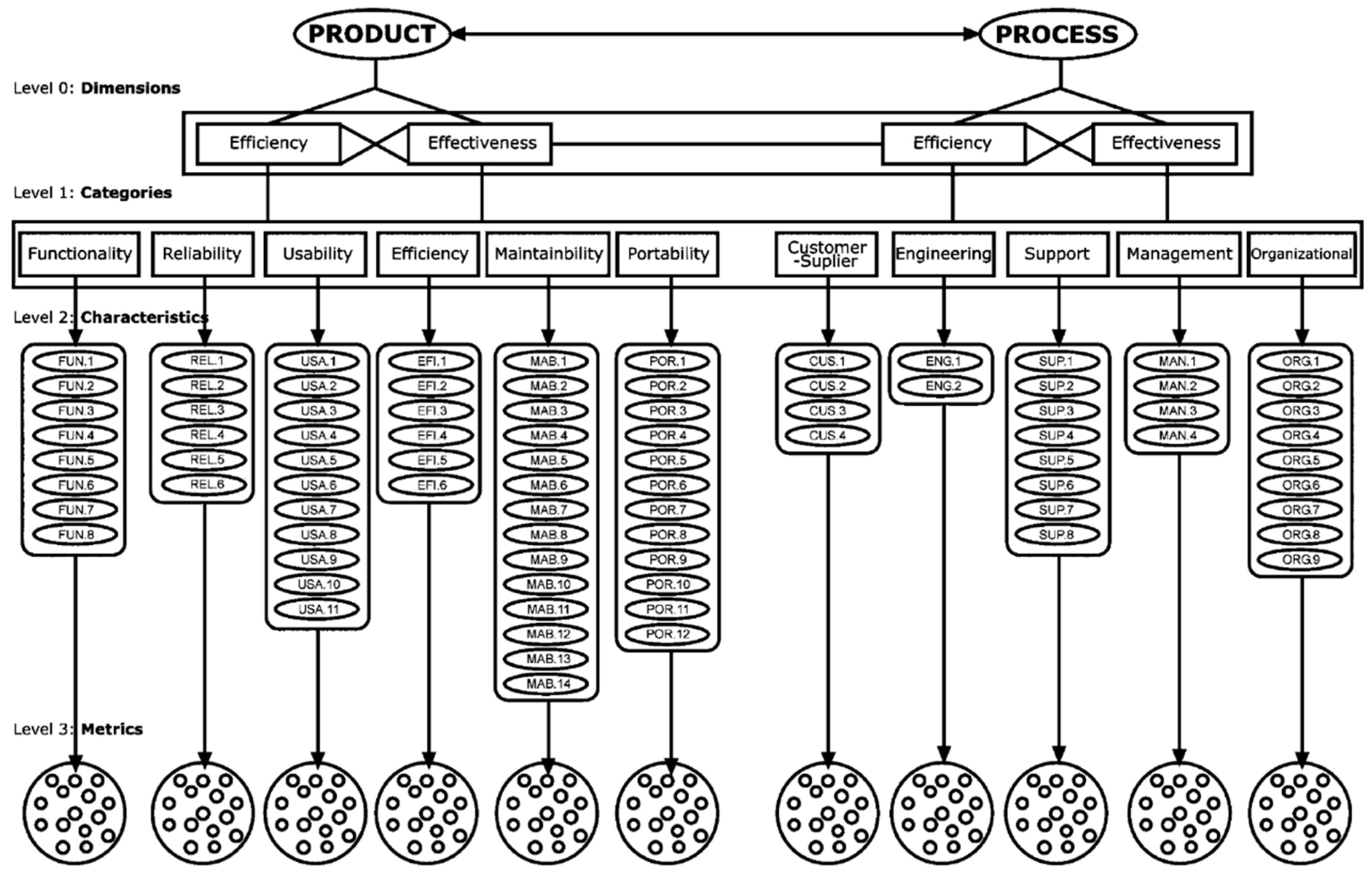
3. Methodology, the Systemic Quality Model (SQMO)
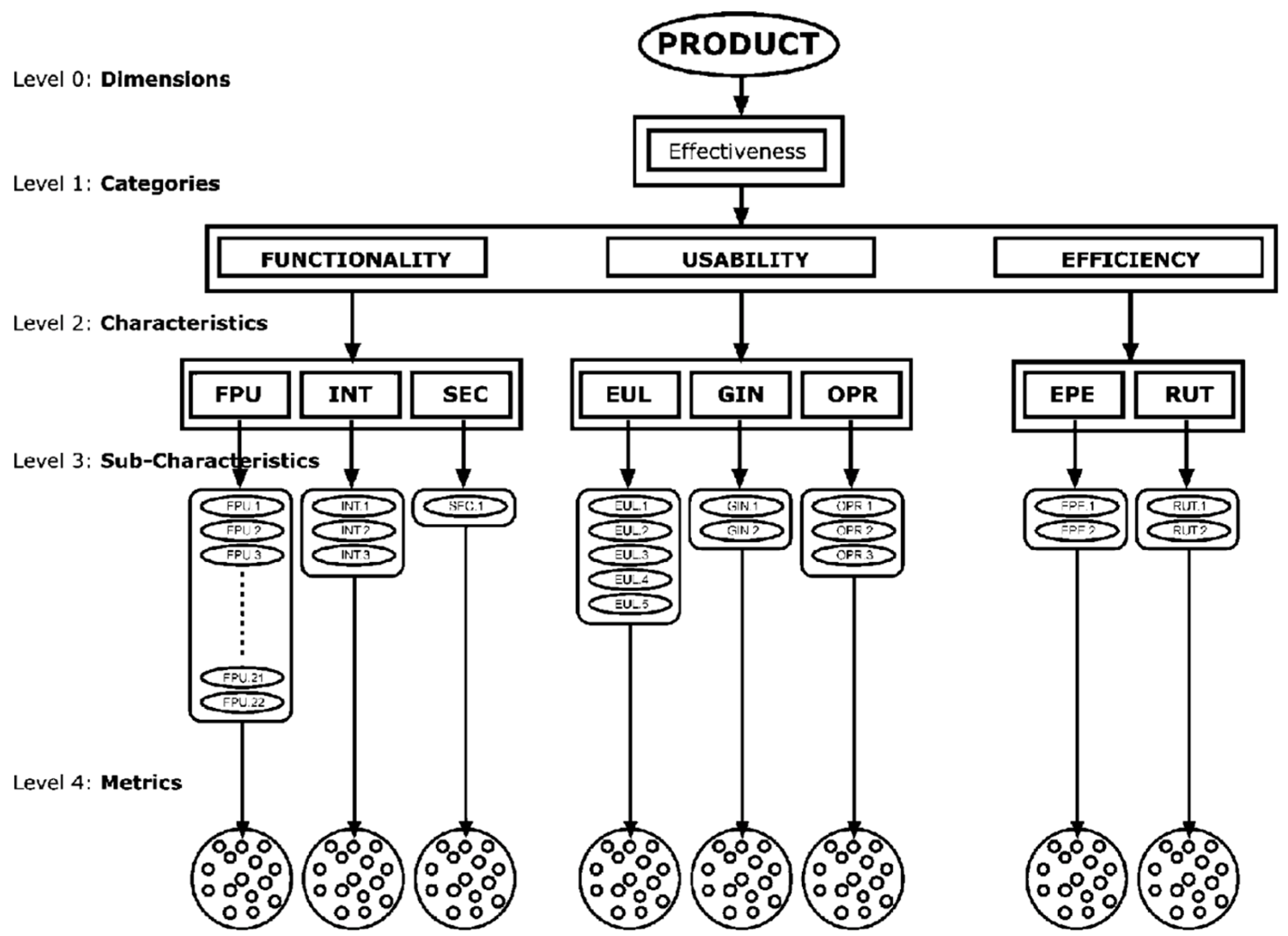
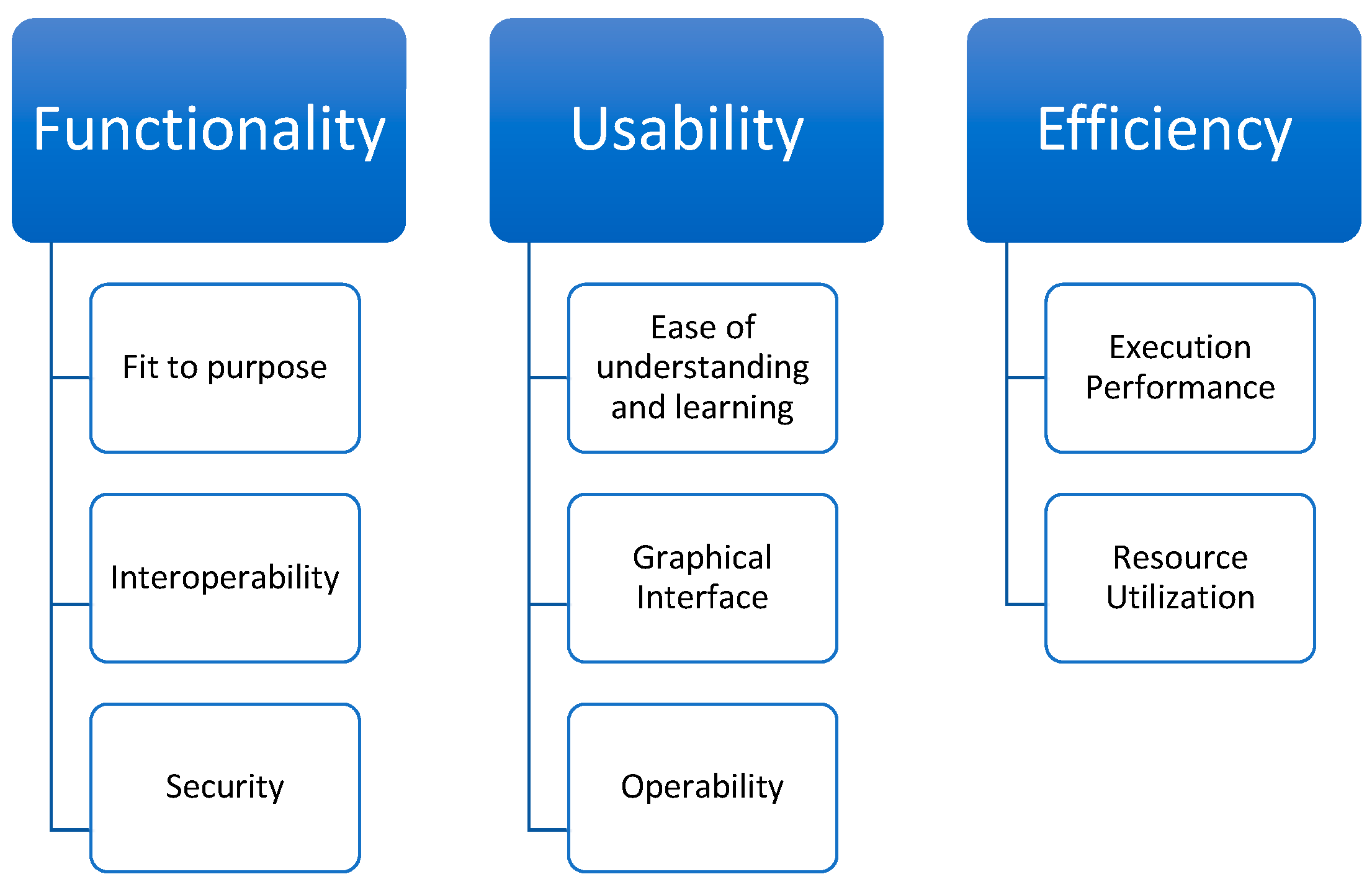
3.1. Level 0: Dimensions
3.2. Level 1: Categories
3.3. Level 2: Characteristics
3.4. Level 3: Metrics
3.5. Algorithm
3.6. Product Software
3.7. Development Process
- Basic level: It is the minimum required level. Categories customer-supplier and engineering are satisfied.
- Medium level: In addition to the basic level categories satisfied, categories support and management are satisfied.
- Advanced level: All categories are satisfied.
4. Adoption of the Systemic Quality Model (SQMO)
5. Scales of Measurement
Type A of Scale Measurement
- 0: The application does not have the feature.
- 1: The application matches the feature poorly or it does not strictly match the feature but it can obtain similar results.
- 2: The application has the feature and matches the expectations, although it needs an extra corporative complement. This mark should also be assigned when the feature implies a manual job (e.g., typing code, clicking a button) and the metric requires an automatic job.
- 3: The application has the feature and matches the expectations successfully without a complement.
- 4: The application has the feature and presents advantages over others.
- 0: Not applicable to the organization.
- 1: Possible feature or wish list item.
- 2: Desired feature.
- 3: Required or must-have feature.
6. The Concept of Satisfaction
Sub-Characteristics and Metrics for Self-Service BI Tools Evaluation
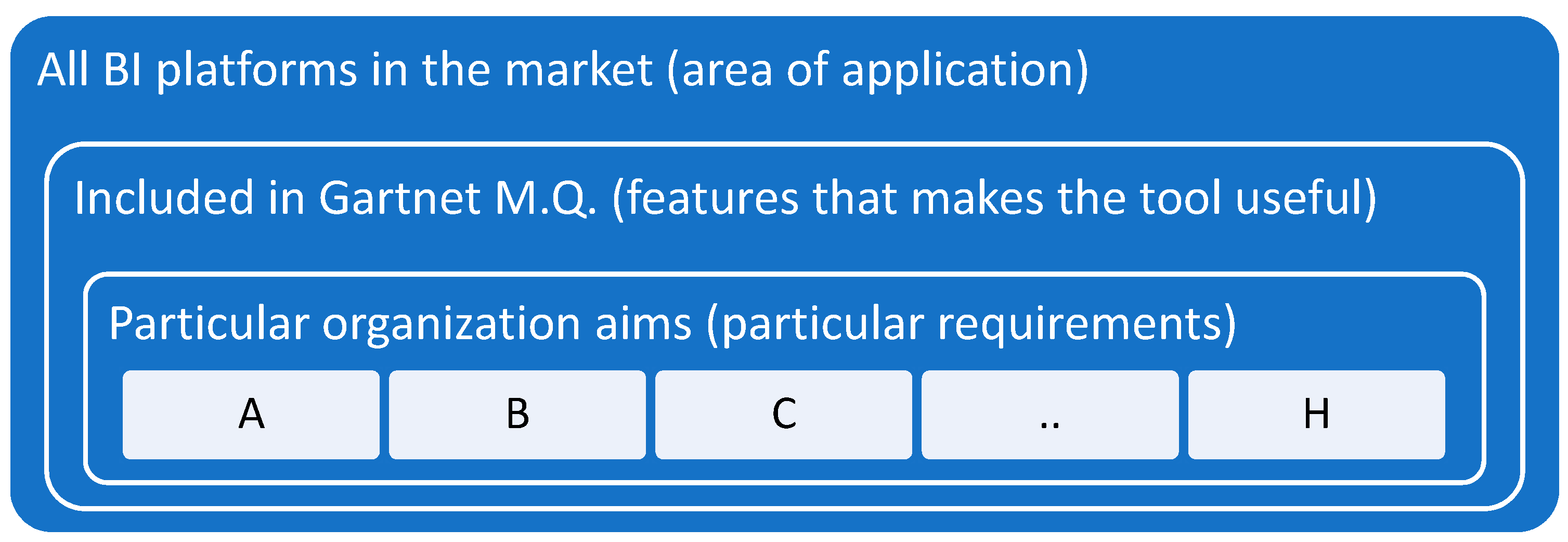
7. Software Selection for the Evaluation
Algorithm
- Functionality and modeling: Diverse source combination and analytical models’ creation of user-defined measures, sets, groups, and hierarchies. Advanced capabilities can include semantic auto discovery, intelligent profiling, intelligent joins, data lineage, hierarchy generation, and data blending from varied data sources, including multi-structured data.
- Internal platform integration: To achieve a common look and feel, and install, query engine, shared metadata, and promo ability across all the components of the platform.
- BI platform administration: Capabilities that enable securing and administering users, scaling the platform, optimizing performance, and ensuring high availability and disaster recovery.
- Metadata management: Tools for enabling users to control the same systems-of-record semantic model and metadata. They should provide a robust and centralized way for administrators to search, capture, store, reuse, and publish metadata objects, such as dimensions, hierarchies, measures, performance metrics/KPIs, and report layout objects.
- Cloud deployment: Platform as a service and analytic application as service capabilities for building, deploying, and managing analytics in the cloud.
- Development and integration: The platform should provide a set of visual tools, programmatic and a development workbench for building dashboards, reports and also queries, and analysis.
- Free-form interactive exploration: Enables the exploration of data through the manipulation of chart images; it must allow changing the color, brightness, size, and shape, and allow to include the motion of visual objects representing aspects of the dataset being analyzed.
- Analytic dashboards and content: The ability to create highly interactive dashboards and content with possibilities for visual exploration. Moreover, the inclusion of geospatial analytics to be consumed by others.
- IT-developed reporting and dashboards: Provides the capability to create highly formatted, print-ready, and interactive reports, with or without a previous parametrization. This includes the ability to publish multi objects, linked reports, and parameters with intuitive and interactive displays.
- Traditional styles of analysis: Ad hoc query that allows users to build their data queries, without relying on IT, to create a report. Specifically, the tools must have a reusable semantic layer that enables users to navigate available data sources, predefined metrics, hierarchies, and so on.
- Mobile: Enables organizations in the development of mobile content and delivers it in a publishing and/or interactive mode.
- Collaboration and social integration: Enables users to share information, analysis, analytic content, and decisions via discussion threads, chat annotations, and storytelling.
- Embedded BI: Resources for modifying and creating analytic content, visualizations, and applications. Resources for embedding this analytic content into a business process and/or an application or portal.
8. The Evaluated Software, the Short List
Data Used
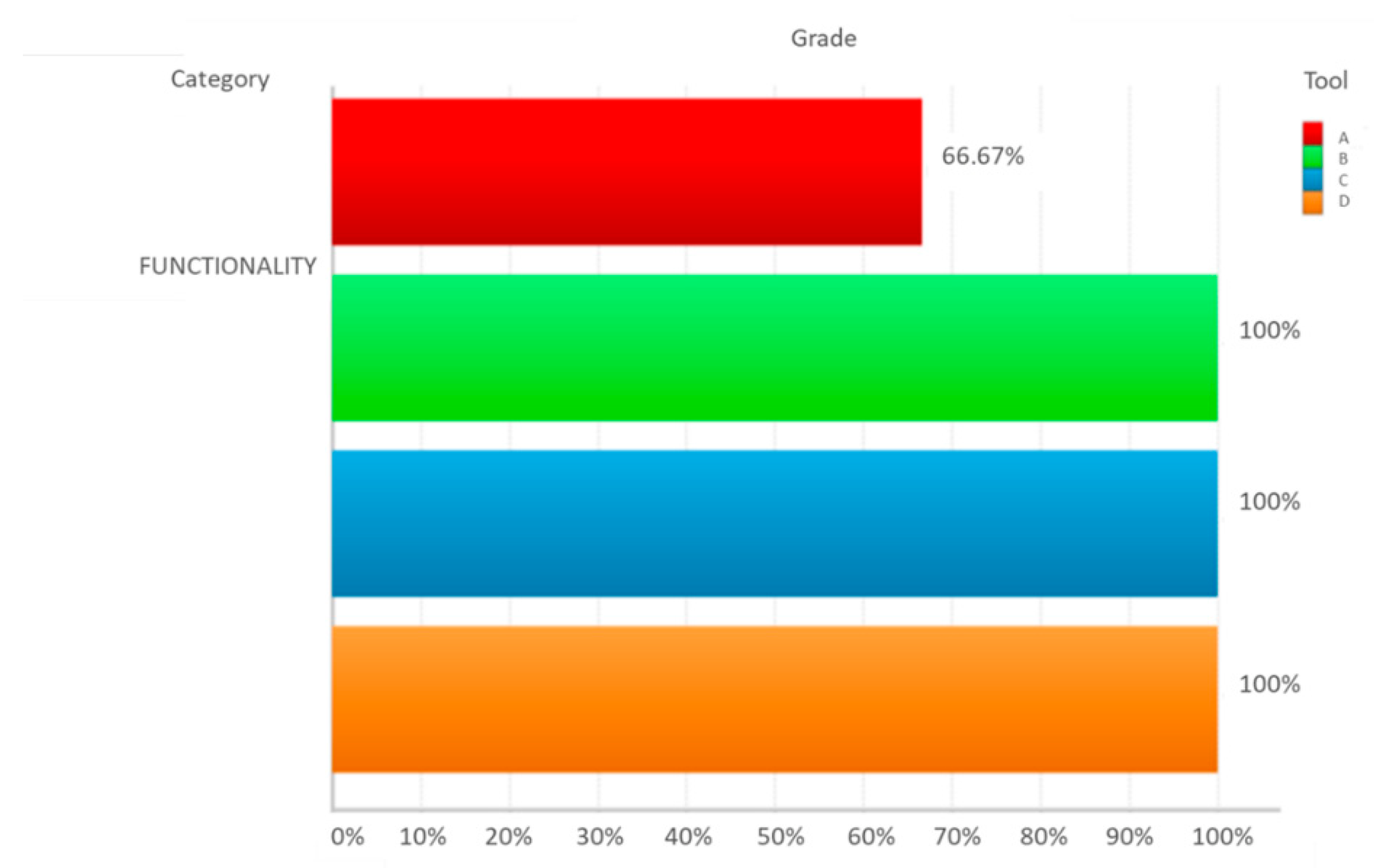
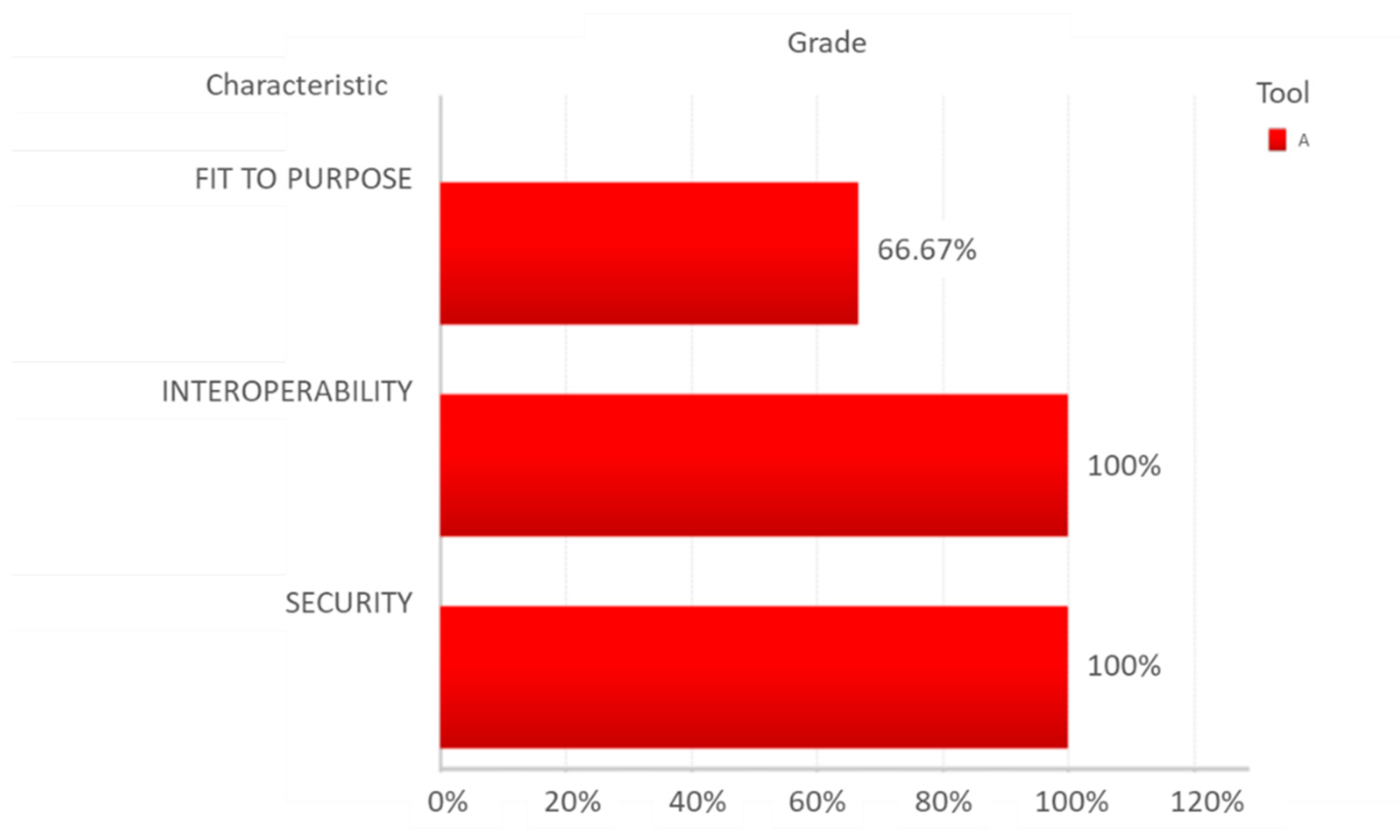
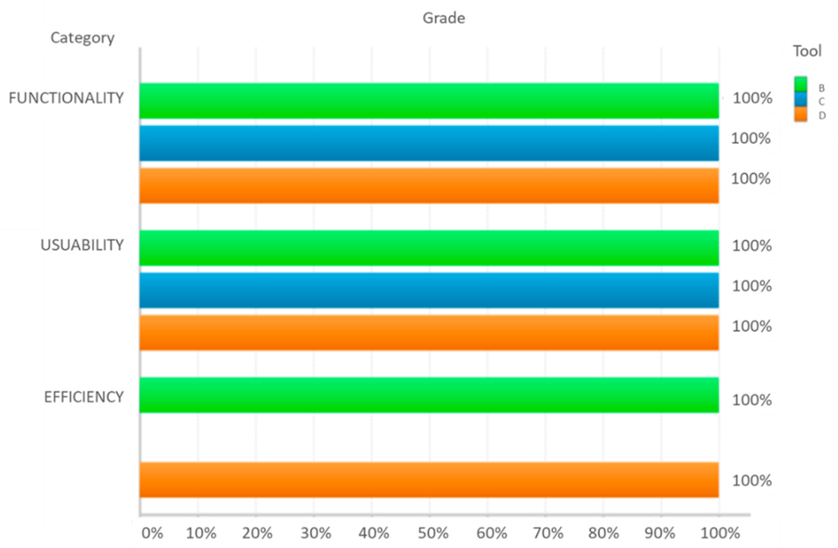
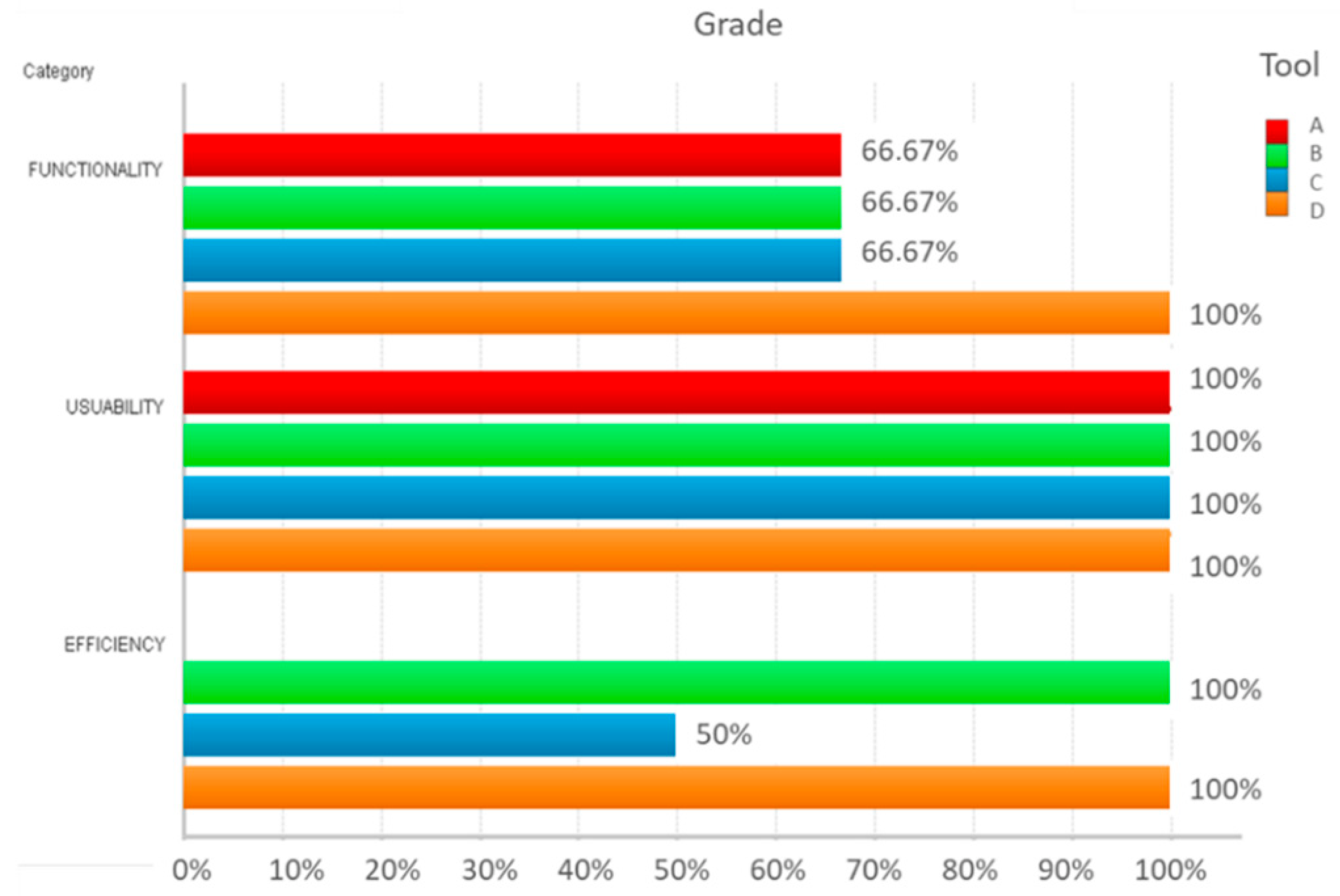
9. Evaluation Results
Results
10. Conclusions
Author Contributions
Funding
Institutional Review Board Statement
Informed Consent Statement
Data Availability Statement
Conflicts of Interest
Appendix A. The Metrics Used in the Selection Process
Appendix A.1. Functionality Category
Appendix A.1.1. Fit to Purpose Characteristic


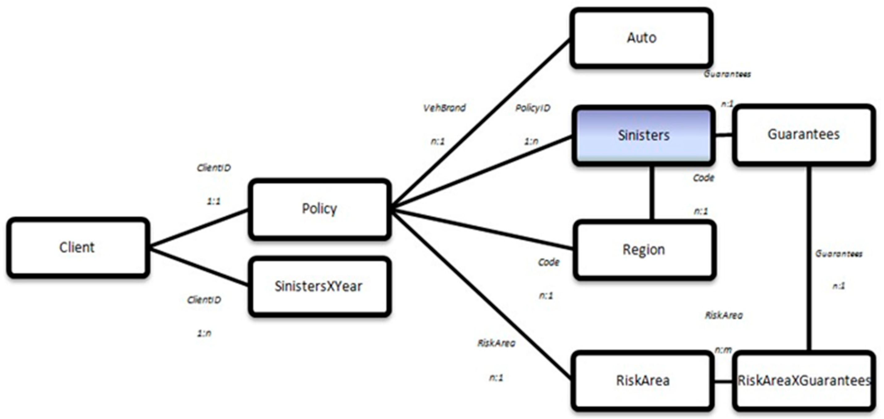
| Policy_id | Code of the Region | Region |
Appendix A.1.2. Interoperability Characteristic
Appendix A.1.3. Security Characteristic
Appendix A.2. Usability Category
Appendix A.2.1. Ease of Understanding and Learning Characteristic
Appendix A.2.2. Graphical Interface Characteristic
Appendix A.2.3. Operability Characteristic
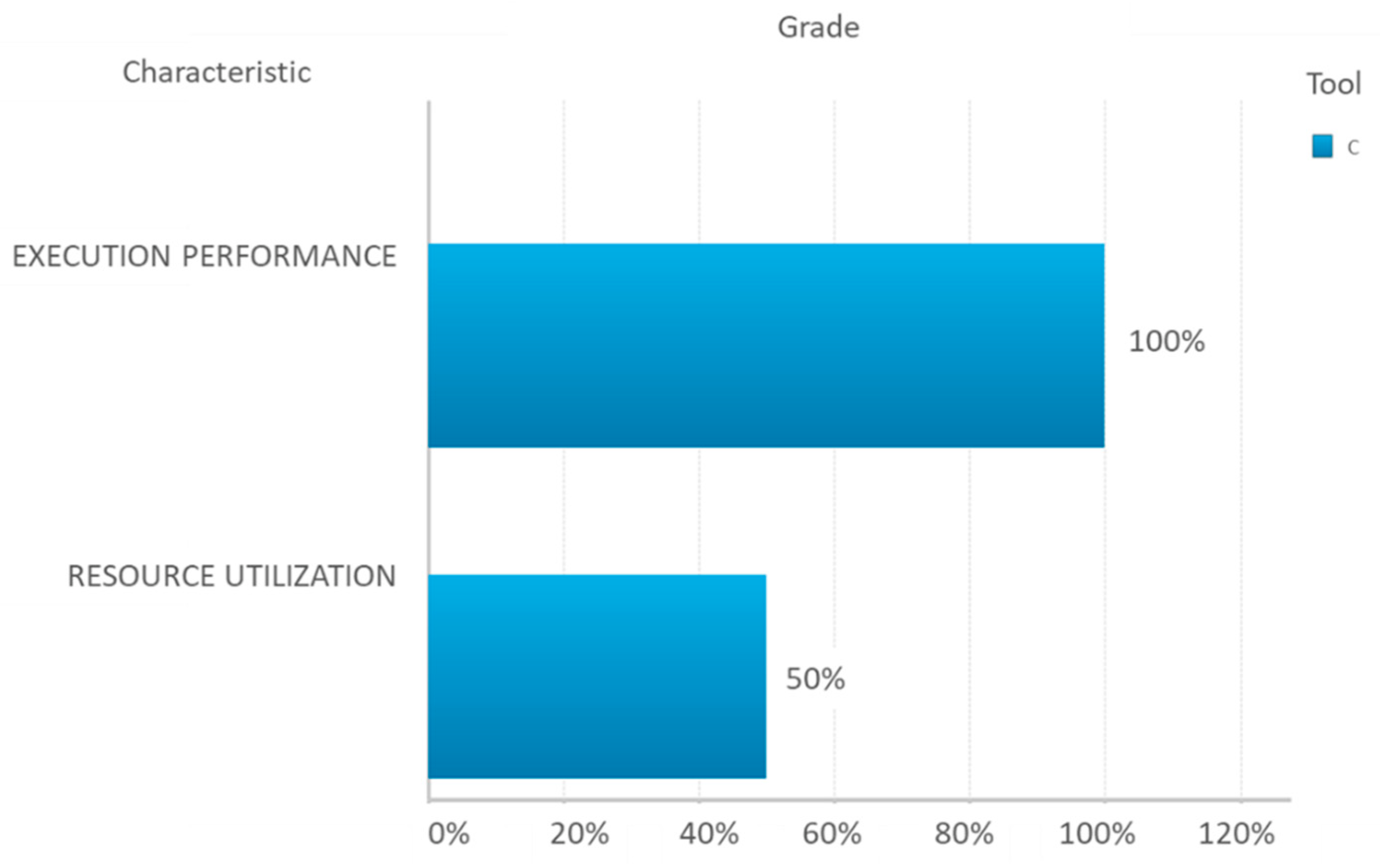
Appendix A.3. Efficiency Category
Appendix A.3.1. Execution Performance Characteristic
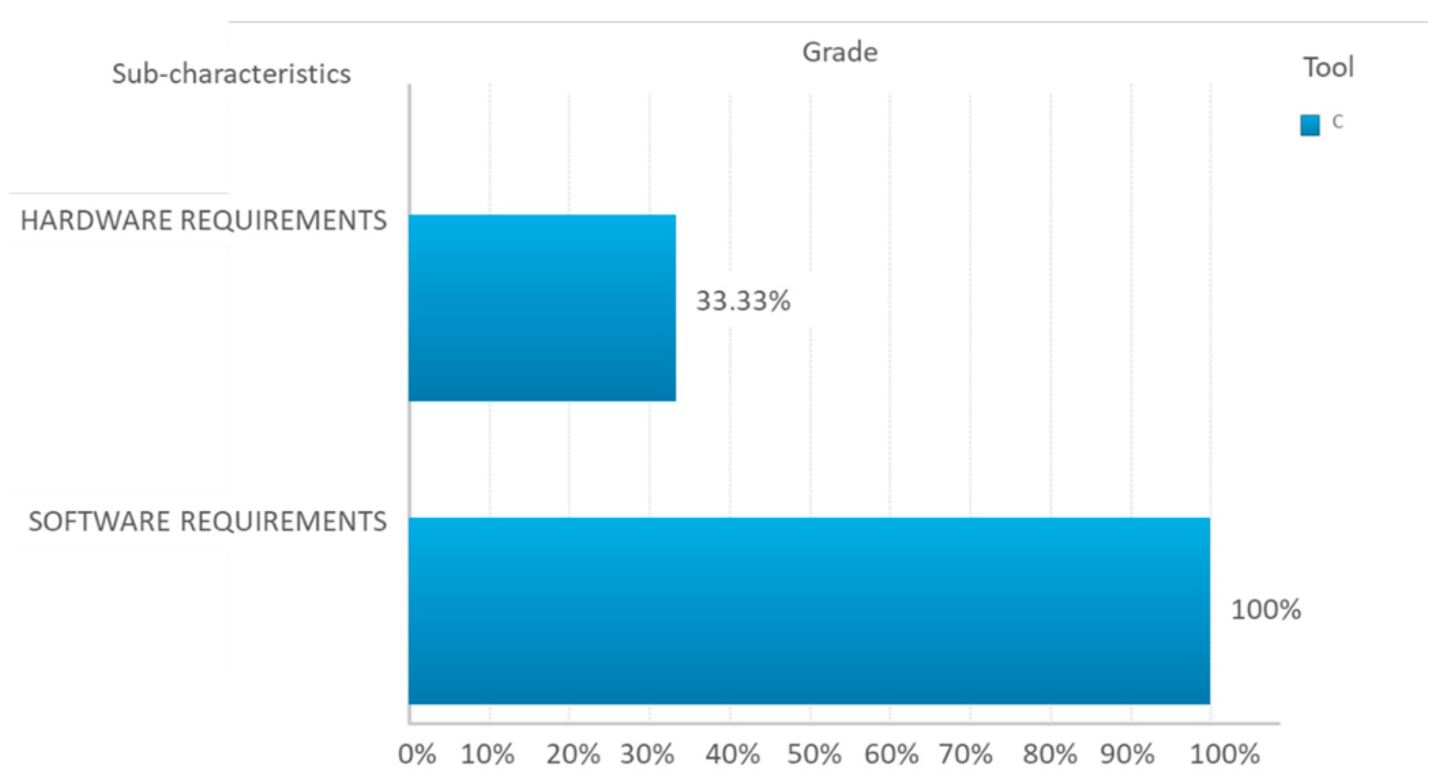
Appendix A.3.2. Resource Utilization Characteristic
Appendix B. Metrics Weights
| Metric | Weight |
|---|---|
| Direct connection to data sources | 2 |
| Bigdata sources | 1 |
| Apache Hadoop | 1 |
| Microsoft Access | 2 |
| Excel files | 3 |
| From an excel file, import all sheets at the same time | 2 |
| Cross-tabs | 2 |
| Plain text | 3 |
| Connecting to different data sources at the same time | 2 |
| Easy integration of many data sources | 2 |
| Visualizing data before the loading | 2 |
| Determining data format | 2 |
| Determining data type | 2 |
| Allowing column filtering before the loading | 2 |
| Allowing row filtering before the loading | 2 |
| Automatic measures creation | 3 |
| Allow renaming datasets | 2 |
| Allow renaming fields | 3 |
| Data cleansing | 2 |
| The data model is done automatically | 2 |
| The done data model is the correct one | 2 |
| The data model can be visualized | 3 |
| Alerting about circular references | 3 |
| Skipping with circular references | 3 |
| The same table can be used several times | 2 |
| Creating new measures based on previous measures | 3 |
| Creating new measures based on dimensions | 3 |
| Variety of functions | 3 |
| Descriptive statistics | 2 |
| Prediction functions | 2 |
| R connection | 2 |
| Geographic information | 2 |
| Time hierarchy | 3 |
| Creating sets of data | 2 |
| Filtering data by expression | 3 |
| Filtering data by dimension | 3 |
| Visual perspective linking | 2 |
| No null data specifications | 2 |
| Considering nulls | 3 |
Appendix C. 0141220_Initial_Test
Appendix C.1. Client Table
- ClientID: Discrete variable with 26,000 different values from 1 to 26,000.
- Gender: Qualitative variable that can take the answers “Male” and “Female”.
- Maristat: Qualitative variable that can take the answers “Others” and “Alone”.
- CSP: Qualitative variable referenced to the social category known as CSP in France. It can take values as “CSP50”. The classification of socio-professional categories (CSP) was conceived by INSEE in 1954. The objective was to categorize individuals according to their professional situation, taking account of several criteria: their profession, economic activity, qualification, hierarchical position and status.
- It included 9 main groups subdivided into 30 socio-professional categories.
- LicBeg: Date variable with 26,000 values between “5 September 1941” and “11 January 2009”. It refers to the date when the client got the driver’s license.
- DrivBeg: Date variable with 26,000 values between “25 January 1916” and “6 January 1991”. It refers to the birth date client.
Appendix C.2. Auto Table
- VehBrand: Categorized numeric variable that refers to the vehicle brand. It takes 11 different values from {1, 2, 3, 4, 5, 6, 10, 11, 12, 13, 14}.
- VehPow: Categorized numeric variable that refers to the vehicle power. It takes 4 different values from {6, 7, 8, 9 }.
- VehType: Qualitative variable that refers to the vehicle type. There are 4 possible answers: “familiar”, “compact”, “sport” and “terrain”.
Appendix C.3. Region Table
- Code: Numeric variable which refers to a code for each region. For example, Zaragoza has the code 52, because it is the last region if they are ordered alphabetically.
- Region: Qualitative variable that refers to the Spain province(region) where the sinister happens. The answers can be: “Alava”, “Albacete”, “Alicante”, “Almeria”, “Asturias”, “Avila”, “Badajoz”, “Barcelona”, “Burgos”, “Caceres”, “Cadiz”, “Cantabria”, “Castellon”, “Ciudad Real”, “Cordoba”, La Coruna”, “Cuenca”, “Gerona”, “Granada”, “Guadalajara”, “Guipuzcoa”, “Huelva”, “Huesca”, “Islas Baleares”, “Jaen”, “Leon”, “Lerida”, “Lugo”, “Madrid”, “Malaga”, “Murcia”, “Navarra”, “Orense”, “Palencia”, “Palmas”, “Pontevedra”, “La Rioja”, “Salamanca”, “Segovia”, “Sevilla”, “Soria”, “Tarragona”, “Teruel”, “Tenerife”, “Toledo”, “Valencia”, “Valladolid”, “Vizacaia”, “Zamora”, “Zaragoza”, “Melilla” and “Ceuta”.is a the whole name of the region, in last example region should be “Zaragoza”.
- Population: Discrete variable that refers to the population of the region where the car is declared.
Appendix C.4. Risk Area Table
- RiskArea: Categorized variable meaning the type of insurance included in each policy, also known as the product. The categories are {1,2,3,4,5}.
- RiskAreadesc: Qualitative variable referring to the corresponding Risk Area name. They are “gold”, “silver”, “master”, “plus” and “regular”.
Appendix C.5. Guarantees Table
- Guarantees: Qualitative variable referring to guarantees with the following possible answers: “windows”, “travelling”, “driver insurance”, “claims”, “fire”, “theft”, “total loss”, and “health assistant”.
- Base: Discrete Variable refers to the cost covered by the insurance company. It has 8 different values: 50, 500, 100, 25, 1000, 20,000, 3000 and 300.
Appendix C.6. Risk X Guarantees Table
- RiskArea: Categorized variable meaning the type of insurance included in each policy, also known as the product. The categories are {1,2,3,4,5}.
- Guarantees: Qualitative variable referring to guarantees provided by the Risk Area corresponding. The different answers are “windows”, “travelling”, “driver insurance”, “claims”, “fire”, “theft”, “total loss” and “ health assistance”.
Appendix C.7. Policy Table
- PolicyID: Discrete variable with 26,000 different values from 1 to 26,000.
- ClientID: Discrete variable with 26,000 different values from 1 to 26,000.
- RecordBeg: Date variable with 26,000 values between “1 January 2000” and “31 December 2010”. It refers to the date when the policy is begun.
- RecordEnd: Date variable with 26,000 values between “1 January 2000” and “31 December 2010”. It refers to the date when the policy is finished. In most cases, it has the value “1 January 9999”, which means that the policy is still active.
- VehBeg: Date variable with 26,000 values between “26 January 1911” and “1 January 2011”. It refers to the date when the vehicle was built.
- VehBrand: Categorized numeric variable that refers to the brand of the secured vehicle, by the policy. It takes 11 different values from {1, 2, 3, 4, 5, 6, 10, 11, 12, 13, 14}.
- BonusMalus: Discrete variable between 50 and 350: below 100 means bonus, above 100 means malus in France.
- RiskArea: Categorized variable meaning the type of insurance included in each policy, also known as the product. The categories are {1, 2, 3, 4, 5}.
- Code: Numeric variable which refers to the code of the region where the policy is registered.
Appendix C.8. SinistersXYear Table
Appendix C.9. Sinisters Table
- PolicyID: Discrete variable with 26,000 different values from 1 to 26,000. However, in the table, every policy is repeated as times as sinister has it in the total of 11 years.
- RiskArea: Categorized variable meaning the type of insurance included in each policy, also known as the product. The categories are {1,2,3,4,5}. As the PolicyID, it is repeated as times as the policy uses the risk area that has been included.
- Guarantees: Qualitative variable referring to a guarantee provided by the Risk Area corresponding and used in the sinister. The different answers are “windows”, “travelling”, “driver insurance”, “claims”, “fire”, “theft”, “total loss” and “ health assistance”.
- Sinisterdate: Date variable with values between “1 January 2000” and “31 December 2010”. It refers to the date when the sinister happens.
- Code: Numeric variable which refers to the code of the region where the sinister happens.
| Variable Name in Simulation | Table | Variable Name |
|---|---|---|
| VehBrand_N | Policy | VehBrand |
| RiskArea_N | Policy | RiskArea |
| Code_O | Policy | Code |
| V1,…, V11 | SinistersXYear | 2000, …, 2010 |
| PolicyID_S | Sinisters | PolicyID |
| RiskArea_s | Sinisters | RiskArea |
| Guarantees_s | Sinisters | Guarantees |
| Code_S | Sinisters | Code |
Appendix D. Questionnaires
| Category | Characteristic | Subcharacteristic-Desc | Metric-Code | Metric | M.S | Value | Weight | Compensated Value | Normal.Value | Indicator_Metric | Total Sub-Characteristic | Indicator_Sub-Charac. | Total Characteristic | Indicator_Charac | Total Category | Indicator_ Categ. |
|---|---|---|---|---|---|---|---|---|---|---|---|---|---|---|---|---|
| Functionality | Fit to Purpose | Data loading | FFI1 | Direct connection to data sources | A | 2 | 2 | 4 | 50.00% | 1 | 82.50% | 1 | 83.33% | 1 | 66.67% | 0 |
| FFI2 | BigData sources | A | 2 | 1 | 2 | 50.00% | 1 | |||||||||
| FFI3 | Apache Hadoop | A | 2 | 1 | 2 | 50.00% | 1 | |||||||||
| FFI4 | Microsoft Access | A | 2 | 2 | 4 | 50.00% | 1 | |||||||||
| FFI5 | Excel files | A | 3 | 3 | 9 | 75.00% | 1 | |||||||||
| FFI6 | From an excel file, import all sheets at the same time | A | 1 | 2 | 2 | 25.00% | 0 | |||||||||
| FFI7 | Cross-tabs | A | 4 | 2 | 8 | 100.00% | 1 | |||||||||
| FFI8 | Plain text | A | 3 | 3 | 9 | 75.00% | 1 | |||||||||
| FFI9 | Connecting to different data sources at the same time | A | 3 | 2 | 6 | 75.00% | 1 | |||||||||
| FFI10 | Easy integration of many data sources | A | 3 | 2 | 6 | 75.00% | 1 | |||||||||
| FFI11 | Visualizing data before the loading | A | 1 | 2 | 2 | 25.00% | 0 | |||||||||
| FFI12 | Determining data format | A | 3 | 2 | 6 | 75.00% | 1 | |||||||||
| FFI13 | Determining data type | A | 4 | 2 | 8 | 100.00% | 1 | |||||||||
| FFI14 | Allowing column filtering before the loading | A | 3 | 2 | 6 | 75.00% | 1 | |||||||||
| FFI15 | Allowing row filtering before the loading | A | 2 | 2 | 4 | 50.00% | 1 | |||||||||
| FFI16 | Automatic measures creation | A | 0 | 3 | 0 | 0.00% | 0 | |||||||||
| FFI17 | Allow renaming datasets | A | 3 | 2 | 6 | 75.00% | 1 | |||||||||
| FFI18 | Allow renaming fields | A | 3 | 3 | 9 | 75.00% | 1 | |||||||||
| FFI19 | Data cleansing | A | 2 | 2 | 4 | 50.00% | 1 | |||||||||
| Data model | FFD1 | The data model is done automatically | A | 3 | 2 | 6 | 75.00% | 1 | 100.00% | 1 | ||||||
| FFD2 | The done data model is the correct one | A | 2 | 2 | 4 | 50.00% | 1 | |||||||||
| FFD3 | The data model can be visualized | A | 4 | 3 | 12 | 100.00% | 1 | |||||||||
| Field relations | FFF1 | Alerting about circular references | A | 3 | 3 | 9 | 75.00% | 1 | 75.00% | 1 | ||||||
| FFF2 | Skipping with circular references | A | 3 | 3 | 9 | 75.00% | 1 | |||||||||
| FFF3 | The same table can be used several times | A | 0 | 2 | 0 | 0.00% | 0 | |||||||||
| Analysis | FFA1 | Creating new measures based on previous measures | A | 3 | 3 | 9 | 75.00% | 1 | 73.33% | 1 | ||||||
| FFA2 | Creating new measures based on dimensions | A | 3 | 3 | 9 | 75.00% | 1 | |||||||||
| FFA3 | Variety of functions | A | 3 | 3 | 9 | 75.00% | 1 | |||||||||
| FFA4 | Descriptive statistics | A | 3 | 2 | 6 | 75.00% | 1 | |||||||||
| FFA5 | Prediction functions | A | 0 | 2 | 0 | 0.00% | 0 | |||||||||
| FFA6 | R connection | A | 3 | 2 | 6 | 75.00% | 1 | |||||||||
| FFA7 | Geographic information | A | 2 | 2 | 4 | 50.00% | 1 | |||||||||
| FFA8 | Time hierarchy | A | 2 | 3 | 6 | 50.00% | 1 | |||||||||
| FFA9 | Creating sets of data | A | 1 | 2 | 2 | 25.00% | 0 | |||||||||
| FFA10 | Filtering data by expression | A | 1 | 3 | 3 | 25.00% | 0 | |||||||||
| FFA11 | Filtering data by dimension | A | 1 | 3 | 3 | 25.00% | 0 | |||||||||
| FFA12 | Visual Perspective Linking | A | 4 | 2 | 8 | 100.00% | 1 | |||||||||
| FFA13 | No Null data specifications | A.1 | 0 | 2 | 0 | 0.00% | 0 | |||||||||
| FFA14 | Considering nulls | A | 4 | 3 | 12 | 100.00% | 1 | |||||||||
| FFA15 | Variety of graphs | A | 3 | 3 | 9 | 75.00% | 1 | |||||||||
| FFA16 | Modify graphs | A | 4 | 3 | 12 | 100.00% | 1 | |||||||||
| FFA17 | No limitations to displaying large amounts of data | A.1 | 4 | 2 | 8 | 100.00% | 1 | |||||||||
| FFA18 | Data refresh | A | 2 | 2 | 4 | 50.00% | 1 | |||||||||
| Dashboards | FFD1 | Dashboards Exportation | A | 3 | 3 | 9 | 75.00% | 1 | 71.43% | 1 | ||||||
| FFD2 | Templates | A | 0 | 2 | 0 | 0.00% | 0 | |||||||||
| FFD3 | Free design | A | 4 | 2 | 8 | 100.00% | 1 | |||||||||
| Reporting | FFR1 | Reports Exportation | A | 3 | 3 | 9 | 75.00% | 1 | 42.86% | 0 | ||||||
| FFR2 | Templates | A | 0 | 2 | 0 | 0.00% | 0 | |||||||||
| FFR3 | Free design | A | 1 | 2 | 2 | 25.00% | 0 | |||||||||
| Interoperability | Languages | FIL1 | Languages displayed | A.1 | 4 | 2 | 8 | 100.00% | 1 | 100.00% | 1 | 75.00% | 0 | |||
| Portability | FIP1 | Operating Systems | A.1 | 0 | 2 | 0 | 0.00% | 0 | 40.00% | 0 | ||||||
| FIP2 | SaaS/Web | A | 1 | 1 | 1 | 25.00% | 0 | |||||||||
| FIP3 | Mobile | A | 3 | 2 | 6 | 75.00% | 1 | |||||||||
| Using the project in third parts | FIU1 | Using the project by third parts | A | 3 | 2 | 6 | 75.00% | 1 | 75.00% | 1 | ||||||
| Data exchange | FID1 | Exportation in txt | A | 3 | 2 | 6 | 75.00% | 1 | 100.00% | 1 | ||||||
| FID2 | Exportation in CSV | A | 3 | 2 | 6 | 75.00% | 1 | |||||||||
| FID3 | Exportation in HTML | A | 3 | 2 | 6 | 75.00% | 1 | |||||||||
| FID4 | Exportation in Excel file | A | 3 | 3 | 9 | 75.00% | 1 | |||||||||
| Security | Security devices | FSS1 | Password protection | A | 3 | 3 | 9 | 75.00% | 1 | 100.00% | 1 | 100.00% | 1 | |||
| FSS2 | Permissions | A | 3 | 3 | 9 | 75.00% | 1 | |||||||||
| Usability | Ease of Understanding and Learning | Learning time | UEL1 | Average learning time | A.2 | 4 | 3 | 12 | 100.00% | 1 | 100.00% | 1 | 100.00% | 1 | 100.00% | 1 |
| Browsing facilities | UEB1 | Consistency between icons in the toolbars and their actions | A | 3 | 3 | 9 | 75.00% | 1 | 100.00% | 1 | ||||||
| UEB2 | Displaying right-click menus | A | 3 | 3 | 9 | 75.00% | 1 | |||||||||
| Terminology | UET1 | Ease of understanding the terminology | A | 4 | 3 | 12 | 100.00% | 1 | 100.00% | 1 | ||||||
| Help and documentation | UEH1 | User guide quality | A.2 | 3 | 2 | 6 | 75.00% | 1 | 100.00% | 1 | ||||||
| UEH2 | User guide acquisition | A | 3 | 2 | 6 | 75.00% | 1 | |||||||||
| UEH3 | On-line documentation | A | 3 | 2 | 6 | 75.00% | 1 | |||||||||
| Support training | UES1 | Availability of tailor-made training courses | A | 3 | 2 | 6 | 75.00% | 1 | 100.00% | 1 | ||||||
| UES2 | Phone technical support | A | 3 | 2 | 6 | 75.00% | 1 | |||||||||
| UES3 | Online support | A | 3 | 2 | 6 | 75.00% | 1 | |||||||||
| UES4 | Availability of consulting services | A | 3 | 2 | 6 | 75.00% | 1 | |||||||||
| UES5 | Free formation | A | 3 | 2 | 6 | 75.00% | 1 | |||||||||
| UES6 | Community | A | 3 | 2 | 6 | 75.00% | 1 | |||||||||
| Graphical Interface Characteristic | Windows and mouse interface | UGW1 | Editing elements by double-clicking | A | 0 | 2 | 0 | 0.00% | 0 | 50.00% | 1 | 100.00% | 1 | |||
| UGW2 | Dragging and dropping elements | A | 3 | 2 | 6 | 75.00% | 1 | |||||||||
| Display | UGD1 | Editing the screen layout | A | 3 | 2 | 6 | 75.00% | 1 | 75.00% | 1 | ||||||
| Operability | Versatility | UOV1 | Automatic update | A | 2 | 2 | 4 | 50.00% | 1 | 50.00% | 1 | 100.00% | 1 | |||
| Efficiency | Execution Performance | Compilation speed | EEC1 | Compilation Speed | A.2 | 4 | 2 | 8 | 100.00% | 1 | 100.00% | 1 | 100.00% | 1 | 100.00% | 1 |
| Resource Utilization | Hardware requirements | ERH1 | CPU(processor type) | A.1 | 4 | 2 | 8 | 100.00% | 1 | 100.00% | 1 | 100.00% | 1 | |||
| ERH2 | Minimum RAM | A.2 | 3 | 2 | 6 | 75.00% | 1 | |||||||||
| ERH3 | Hard disk space required | A.2 | 4 | 2 | 8 | 100.00% | 1 | |||||||||
| Software requirements | ERS1 | Additional software requirements | A | 4 | 2 | 8 | 100.00% | 1 | 100.00% | 1 |
References
- Hass, K.B.; Lindbergh, L.; Vanderhorst, R.; Kiemski, K. From Analyst to Leader: Elevating the Role of the Business Analyst Management Concepts; Berrett-Koehler Publishers: Oakland, CA, USA, 2007; p. 152. [Google Scholar]
- International Institute of Business Analysis. The Guide to the Business Analysis Body of Knowledge TM; International Institute of Business Analysis: London UK, 2012. [Google Scholar]
- Pollock, N.; Williams, R. Technology choice and its performance: Towards a sociology of software package procurement. Inf. Organ. 2007, 17, 131–161. Available online: http://www.sciencedirect.com/science/article/pii/S147177270700022X (accessed on 9 July 2022). [CrossRef] [Green Version]
- Zaidan, A.A.; Zaidan, B.B.; Hussain, M.; Haiqi, A.; Mat Kiah, M.L.; Abdulnabi, M. Multi-criteria analysis for OS-EMR software selection problem: A comparative study. Decis. Support Syst. 2015, 78, 15–27. Available online: http://linkinghub.elsevier.com/retrieve/pii/S0167923615001347 (accessed on 9 July 2022). [CrossRef]
- Sudhaman, P.; Thangavel, C. Efficiency analysis of ERP projects—Software quality perspective. Int. J. Proj. Manag. 2015, 33, 961–970. Available online: http://linkinghub.elsevier.com/retrieve/pii/S0263786314001689 (accessed on 9 July 2022). [CrossRef]
- Yazgan, H.R.; Boran, S.; Goztepe, K. An ERP software selection process with using artificial neural network based on analytic network process approach. Expert. Syst. Appl. 2009, 36, 9214–9222. Available online: http://www.sciencedirect.com/science/article/pii/S0957417408008877 (accessed on 9 July 2022). [CrossRef]
- Gürbüz, T.; Alptekin, S.E.; Işıklar Alptekin, G. A hybrid MCDM me thodology for ERP selection problem with interacting criteria. Decis. Support Syst. 2012, 54, 206–214. Available online: http://linkinghub.elsevier.com/retrieve/pii/S0167923612001170 (accessed on 9 July 2022). [CrossRef]
- Bao, T.; Liu, S. Quality evaluation and analysis for domain software: Application to management information system of power plant. Inf. Softw. Technol. 2016, 78, 53–65. Available online: http://linkinghub.elsevier.com/retrieve/pii/S0950584916300933 (accessed on 9 July 2022). [CrossRef]
- Koh, S.C.L.; Gunasekaran, A.; Goodman, T. Drivers, barriers and critical success factors for ERPII implementation in supply chains: A critical analysis. J. Strateg. Inf. Syst. 2011, 20, 385–402. Available online: http://linkinghub.elsevier.com/retrieve/pii/S0963868711000400 (accessed on 9 July 2022). [CrossRef]
- Abu Salih, B.; Wongthongtham, P.; Beheshti, S.M.R.; Zajabbari, B. Towards a Methodology for Social Business Intelligence in the Era of Big Social Data Incorporating Trust and Semantic Analysis. Lect. Notes Electr. Eng. 2019, 520, 519–527. [Google Scholar]
- Wongthongtham, P.; Salih, B.A. Ontology and Trust based Data Warehouse in New Generation of Business Intelligence. IEEE 13th Int. Conf. Ind. Inform. 2015, Idc, 476–483. [Google Scholar]
- Arvidsson, V.; Holmström, J.; Lyytinen, K. Information systems use as strategy practice: A multi-dimensional view of strategic information system implementation and use. J. Strateg. Inf. Syst. 2014, 23, 45–61. Available online: http://linkinghub.elsevier.com/retrieve/pii/S0963868714000055 (accessed on 9 July 2022). [CrossRef] [Green Version]
- Kovtun, V.; Izonin, I.; Gregus, M. The functional safety assessment of cyber-physical system operation process described by Markov chain. Sci. Rep. 2022, 12, 7089. Available online: https://doi.org/10.1038/s41598-022-11193-w (accessed on 9 July 2022). [CrossRef] [PubMed]
- Kovtun, V.; Izonin, I.; Gregus, M. Model of Information System Communication in Aggressive Cyberspace: Reliability, Functional Safety, Economics. IEEE Access 2022, 10, 31494–31502. [Google Scholar] [CrossRef]
- Mendoza, L.E.; Grimán, A.C.; Rojas, T. Algoritmo para la Evaluación de la Calidad Sistémica del Software. In Proceedings of the 2nd Ibero-American Symposium on Software Engineering and Knowledge Engineering, Salvador, Brasil, October 2002. [Google Scholar]
- Rincon, G.; Alvarez, M.; Perez, M.; Hernandez, S. A discrete-event simulation and continuous software evaluation on a systemic quality model: An oil industry case. Inf. Manag. 2005, 42, 1051–1066. [Google Scholar] [CrossRef]
- Mendoza, L.E.; Pérez, M.A.; Grimán, A.C. Prototipo de Modelo Sistémico de Calidad (MOSCA) del Software 2 Matriz de Calidad Global Sistémica. Comput. Y Sist. 2005, 8, 196–217. [Google Scholar]
- Kirkwood, H.P. Corporate Information Factory; John Wiley & Sons: Hoboken, NJ, USA, 1998; Volume 22, pp. 94–95. Available online: http://search.proquest.com.bibl.proxy.hj.se/docview/199904146/abstract?accountid=11754 (accessed on 9 July 2022).
- Bass, L.; Clements, P.; Kazman, R. Software Architecture in Practice; Addison-Wesley Professional: Boston, MA, USA, 2003; p. 528. [Google Scholar]
- Callaos, N.; Callaos, B. Designing with Systemic Total Quality. Educ. Technol. 1993, 34, 12. [Google Scholar]
- Humphrey, W.S. Introduction to the Personal Software Process; Addison-Wesley Professional: Boston, MA, USA, 1997. [Google Scholar]
- Ortega, M.; Pérez, M.; Rojas, T. A Model for Software Product Quality with a Systemic Focus. Int. Inst. Inform. Syst. 2001, 395–401. [Google Scholar]
- Pérez, M.A.; Rojas, T.; Mendoza, L.E.; Grimán, A.C.; Procesos, D.; Bolívar, U.S. Systemic Quality Model for System Development Process: Case Study. In Proceedings of the AMCIS 2001, Boston, MA, USA, 3–5 August 2001; pp. 1–7. [Google Scholar]
- Dromey, G. Cornering to Chimera. IEEE Softw. 1996, 13, 33–43. [Google Scholar] [CrossRef]
- Kitchenman, B.A.; Jones, L. Evaluating software engineering methods and tool part 5: The influence of human factors. ACM SIGSOFT Softw. Eng. Notes 1997, 22, 13–15. [Google Scholar] [CrossRef]
- Jelassi, T.; Le Blanc, L.A. DSS Software Selection: A multiple Criteria Decision Methodology. Inf. Manag. 1989, 17, 49–65. [Google Scholar]
- Hostmann, B.; Oestreich, T.; Parenteau, J.; Sallam, R.; Schlegel, K.; Tapadinhas, J. Magic Quadrant for Business Intelligence and Analytics Platforms MicroStrategy Positioned in ‘Leaders’ Quadrant. 2013. Available online: http://www.microstrategy.com/about-us/analyst-reviews/gartner-magic-quadrant. (accessed on 9 July 2022).
- Abelló Gamazo, A.; Samos Jiménez, J.; Curto Díaz, J. La Factoría De Información Corporativa; Universitat Oberta de Catalunya: Barcelona, Spain, 2014. [Google Scholar]
- Rincon, G.; Perez, M. Discrete-event Simulation Software Decision Support in the Venezuelan Oil Industry. In Proceedings of the AMCIS 2004 Proceedings, New York, NY, USA, 22 August 2004; Available online: http://aisel.aisnet.org/amcis2004/7 (accessed on 9 July 2022).
| Category | Definition |
|---|---|
| Functionality (FUN) | Functionality is the capacity of the software product to provide functions that meet specific and implicit needs when software is used under specific conditions |
| Reliability (FIA) | Reliability is the capacity of a software product to maintain a specified level of performance when used under specific conditions |
| Usability (USA) | Usability is the capacity of the software product to be attractive, understood, learned, and used by the user under certain specific conditions |
| Efficiency (EFI) | Efficiency is the capacity of a software product to provide appropriate performance, relative to the number of resources used, under stated conditions |
| Maintainability (MAB) | Maintainability is the capacity of the software to be modified. Modifications can include corrections, improvements, or adaptations of the software to adjust to changes in the environment, in terms of the functional requirements and specifications |
| Portability (POR) | Portability is the capacity of the software product to be transferred from one environment to another |
| Category | Definition |
|---|---|
| Client-supplier (CUS) | Is made up of processes that have an impact on the client, support the development and transition of the software to the client, and give the correct operation and use of the software product or service |
| Engineering (ENG) | Consists of processes that directly specify, implement, or maintain the software product, its relation to the system, and documentation on it |
| Support (SUP) | Consists of processes that can be used by any of the processes (including support ones) at several levels of the acquisition life cycle |
| Management (MAN) | Consists of processes that contain practices of a generic nature that can be used by anyone managing any kind of project or process, within a primary life cycle |
| Organizational (ORG) | Contain processes that establish the organization’s commercial goals and develop process, product, and resource goods (value) that will help the organization attain the goals set in the projects |
| Category | Characteristics | |
|---|---|---|
| Product Effectiveness | Product Efficiency | |
| Functionality | Fit to purpose | Correctness |
| Precision | Structured | |
| Interoperability | Encapsulated | |
| Security | Specified | |
| Reliability | Maturity | Correctness |
| Fault tolerance | Structured | |
| Recovery | Encapsulated | |
| Usability | Ease of understanding | Complete |
| Ease of learning | Consistent | |
| Graphical Interface | Effective | |
| Operability | Specified | |
| Conformity of standards | Documented | |
| Auto-descriptive | ||
| Efficiency | Execution performance | Effective |
| Resource utilization | No redundant | |
| Direct | ||
| Used | ||
| Maintainability | Analysis Capability | Attachment |
| Ease of changing | Cohesion | |
| Stability | Encapsulated | |
| Testability | Software maturity | |
| Structure information | ||
| Descriptive | ||
| Correctness | ||
| Structural | ||
| Modularity | ||
| Portability | Adaptability | Consistent |
| Installation capability | Parameterized | |
| Co-existence | Encapsulated | |
| Replacement capability | Cohesive | |
| Specified | ||
| Documented | ||
| Auto-descriptive | ||
| No redundant | ||
| Auditing | ||
| Quality management | ||
| Data Quality -both dimensions- | ||
| Category | Characteristics | |
|---|---|---|
| Process Effectiveness | Process Efficiency | |
| Customer–Supplier | Acquisition system or software product | Supply |
| Requirement determination | Operation | |
| Engineering | Development | Maintenance of software and systems Principio del formulario |
| Support | Quality assurance | Documentation |
| Joint review | Configuration management | |
| Auditing | Verification | |
| Solving problems | Validation | |
| Joint review | ||
| Auditing | ||
| Solving problems | ||
| Management | Management | Management |
| Quality management | Project management | |
| Risk management | Quality management | |
| Risk management | ||
| Organizational | Organizational alignment | Establishment of the process |
| Management of change | Process evaluation | |
| Process improvement | Process improvement | |
| Measurement | HHRR management | |
| Reuse | Infrastructure | |
| Functionality | Second Category | Third Category | Quality Level |
|---|---|---|---|
| Satisfied | No satisfied | No satisfied | Basic |
| Satisfied | Satisfied | No satisfied | Medium |
| Satisfied | No satisfied | Satisfied | Medium |
| Satisfied | Satisfied | Satisfied | Advanced |
| Quality Levels | Category Satisfied | ||
|---|---|---|---|
| Advanced | Medium | Basic | Customer–supplier |
| Engineering | |||
| Support | |||
| Management | |||
| Organizational | |||
| Product Quality Level | Process Quality Level | Systemic Quality Level |
|---|---|---|
| Basic | - | Null |
| Basic | Basic | Basic |
| Medium | - | Null |
| Medium | Basic | Basic |
| Advanced | - | Null |
| Advanced | Basic | Medium |
| Basic | Medium | Basic |
| Medium | Medium | Medium |
| Advanced | Medium | Medium |
| Basic | Advanced | Medium |
| Medium | Advanced | Medium |
| Advanced | Advanced | Advanced |
| Metric | Weight |
|---|---|
| Excel files | 3 |
| Plain text | 3 |
| Connecting to different data sources at the same time | 2 |
| Allow renaming fields | 3 |
| R connection | 2 |
| Geographic information | 2 |
| … |
| Limit for metric | 50% |
| Limit for sub-characteristic | 50% |
| Limit for characteristic | 75% |
| Limit for category | 75% |
| Functionality Category | ||
|---|---|---|
| Fit for purpose | Interoperability | Security |
| Data loading | Languages | Security devices |
| Data model | Use project by third parts | |
| Fields relations | Languages | |
| Analysis | Data exchange | |
| Dashboard | ||
| Reporting | ||
| Usability Category | ||
|---|---|---|
| Ease of understanding and learning | Graphical interface | Operability |
| Learning time | Windows and mouse interface | Versatility |
| Browsing facilities | Display | |
| Terminology | ||
| Help and documentation | ||
| Support and training | ||
| Efficiency Category | |
|---|---|
| Execution performance | Resource utilization |
| Compilation speed | Hardware requirements |
| Software requirements | |
| Adaptive Insights | Birst | DataRPM | FICO | Jedox | Oracle | Salesforce |
| Advizor Solutions | Bitam | Datawatch | GoodData | Kofax(Altosoft) | Palantir Technologies | Salient Management Company |
| AFS Technologies | Board International | Decisyon | IBM Cognos | L-3 | Panorama | SAP |
| Alteryx | Centrifuge Systems | Dimensional Insight | iDashboards | LavaStorm Analytics | Pentaho | SAS (SAS Business Analytics) |
| Antivia | Chartio | Domo | Incorta | Logi Analytics | Platfora | Sisense |
| Arcplan | ClearStory Data | Dundas Data Visualization | InetSoft | Microsoft BI | Prognoz | Splunk |
| Automated Insgihts | DataHero | Eligotech | Infor | MicroStrategy. | Pyramid Analytics | Strategy Comapnio |
| BeyondCore | Datameer | eQ Technologic | Information Builder | Open Text (Actuate) | Qlik | SynerScope |
| Tableau | Targit | ThoughtSpot | Tibco Software | Yellowfin | Zoomdata | Zucche |
| Alteryx | Information Builder | Panorama | SAP (SAP Lumira) |
| Birst | Logi Analytics | Pentaho | SAS (SAS Business Analytics) |
| Board International | Microsoft BI | Prognoz | Tableau |
| Datawatch | MicroStrategy. (MicroStrategy Visual Insight) | Pyramid Analytics | Targit |
| GoodData | Open Text (Actuate) | Qlik (QlikView) | Tibco Software |
| IBM Cognos | Oracle | Salient Management Company | Yellowfin |
| Tool | Functionality | Usability | Efficiency | Quality Level |
|---|---|---|---|---|
| Software B | Satisfied | Satisfied | Satisfied | Advanced |
| Software C | Satisfied | Satisfied | No satisfied | Medium |
| Software D | Satisfied | Satisfied | Satisfied | Advanced |
| Limit for metric | 50% |
| Limit for sub-characteristic | 50% |
| Limit for characteristic | 80% |
| Limit for category | 75% |
Publisher’s Note: MDPI stays neutral with regard to jurisdictional claims in published maps and institutional affiliations. |
© 2022 by the authors. Licensee MDPI, Basel, Switzerland. This article is an open access article distributed under the terms and conditions of the Creative Commons Attribution (CC BY) license (https://creativecommons.org/licenses/by/4.0/).
Share and Cite
Orcajo Hernández, J.; Fonseca i Casas, P. Business Intelligence’s Self-Service Tools Evaluation. Technologies 2022, 10, 92. https://doi.org/10.3390/technologies10040092
Orcajo Hernández J, Fonseca i Casas P. Business Intelligence’s Self-Service Tools Evaluation. Technologies. 2022; 10(4):92. https://doi.org/10.3390/technologies10040092
Chicago/Turabian StyleOrcajo Hernández, Jordina, and Pau Fonseca i Casas. 2022. "Business Intelligence’s Self-Service Tools Evaluation" Technologies 10, no. 4: 92. https://doi.org/10.3390/technologies10040092