An Optimum Load Forecasting Strategy (OLFS) for Smart Grids Based on Artificial Intelligence

Abstract

Recently, the application of Artificial Intelligence (AI) in many areas of life has allowed raising the efficiency of systems and converting them into smart ones, especially in the field of energy. Integrating AI with power systems allows electrical grids to be smart enough to predict the future load, which is known as Intelligent Load Forecasting (ILF). Hence, suitable decisions for power system planning and operation procedures can be taken accordingly. Moreover, ILF can play a vital role in electrical demand response, which guarantees a reliable transitioning of power systems. This paper introduces an Optimum Load Forecasting Strategy (OLFS) for predicting future load in smart electrical grids based on AI techniques. The proposed OLFS consists of two sequential phases, which are: Data Preprocessing Phase (DPP) and Load Forecasting Phase (LFP). In the former phase, an input electrical load dataset is prepared before the actual forecasting takes place through two essential tasks, namely feature selection and outlier rejection. Feature selection is carried out using Advanced Leopard Seal Optimization (ALSO) as a new nature-inspired optimization technique, while outlier rejection is accomplished through the Interquartile Range (IQR) as a measure of statistical dispersion. On the other hand, actual load forecasting takes place in LFP using a new predictor called the Weighted K-Nearest Neighbor (WKNN) algorithm. The proposed OLFS has been tested through extensive experiments. Results have shown that OLFS outperforms recent load forecasting techniques as it introduces the maximum prediction accuracy with the minimum root mean square error.

1. Introduction

Electrical load forecasting is an important process in Smart Electrical Grids (SEGs) [1,2,3]. That is because it can improve the performance of SEGs, stability, reliability, and safety and can reduce the power costs. In SEGs, load forecasting plays an instrumental role in other sectors such as customer demand forecasting and power generation sectors as it provides them with information about the amount of energy needed in the future [4,5]. Electrical companies pay attention to provide continuous and reliable service to their customers [1]. Indeed, higher electrical loads increase the complexity in designing SEGs. Hence, load forecasting is an important process to accurately determine the amount of energy needed in the future. Traditional load forecasting models cannot provide quick and perfect results, therefore, it is important to find a fast and accurate load forecasting model based on artificial intelligence techniques [6,7,8].

Artificial Intelligence (AI) technology plays a major role in many different sectors such as the civil sector, medical sector, telecommunication sector, electricity sector, etc. In SEGs, AI can be used to introduce an improved load forecasting model that gives quick and more accurate results [4,5,9]. There are several AI techniques that can be used to estimate how much power will be required in the future such as Artificial Neural Networks (ANNs), K-Nearest Neighbors (KNNs), Fuzzy Logic (FL), Support Vector Machine (SVM), Naïve Bayes (NB), and Decision Tree (DT) [6]. Despite the effectiveness of these techniques in current research, these techniques cannot reach optimal results in the least possible time for short-term load forecasting. Hence, it is essential to improve these techniques to give fast and accurate predictions. To provide perfect results, preprocessing processes called outlier rejection and feature selection should be performed before using the forecasting model to enable the forecasting model to provide fast and accurate results [6]. That is because irrelevant features and bad items may prevent the load forecasting model from providing accurate results and also may prolong training.

The feature selection process selects the most important features that have an effect on the load and removes irrelevant features [4,5]. It reduces overfitting and gives the load forecasting model the ability to give fast and more accurate results. Feature selection methods are categorized as wrapper, filter, and hybrid [6]. Filter methods are fast but less accurate methods while wrapper methods are accurate but slow methods. Hybrid methods combine filter and wrapper methods to quickly and accurately select the best features. The outlier rejection process eliminates bad items that have a bad effect on the load forecasting model. It enables the load forecasting model to correctly learn and provide accurate results. There are three main categories to classify outlier rejection methods: distance-based methods, cluster-based methods, and statistical-based methods [4,6].

In this paper, a new load forecasting strategy called Optimum Load Forecasting Strategy (OLFS) has been introduced to accurately and quickly forecast loads. OLFS contains two main phases called the Data Preprocessing Phase (DPP) and Load Forecasting Phase (LFP). In the DPP, two main processes called feature selection and outlier rejection are applied to prepare the input electrical dataset before learning the load forecasting model. The feature selection process is performed using a new optimization technique named Advanced Leopard Seal Optimization (ALSO). On the other hand, the outlier rejection process is performed using a statistical-based method called Interquartile Range (IQR). In the LFP, a new load forecasting algorithm called Weighted K-Nearest Neighbor (WKNN) is applied to provide perfect predictions based on the prepared dataset after removing outliers and irrelevant features. Results showed that the proposed OLFS outperforms recent techniques according to accuracy, error, and execution time metrics.

The structure of this paper is arranged as follows: Section 2 introduces the previous work about recent load forecasting techniques. Section 3 discusses the proposed perfect load forecasting strategy in detail and Section 4 provides the experimental results. Finally, conclusions and future works are presented in Section 5.

2. Related Work

In this section, the most recent load forecasting techniques are described. As presented in [1], three deep learning models called Gated Recurrent Unit (GRU), Long Short-Term Memory (LSTM), and Recurrent Neural Network (RNN) algorithms were applied as load forecasting models. Experimental results showed that GRU outperformed LSTM and RNN in terms of R-squared, mean square error, and mean absolute error. GRU is effective and it should be able to predict loads based on new features. Additionally, it should be trained on online datasets collected from smart meters. Feature selection and outlier rejection methods were not used before applying the prediction model. In [2], the Hybrid Forecasting Model (HFM) was proposed to forecast loads and prices. In fact, the HFM consists of two main methods called the Bidirectional Long Short-Term Memory with Attention Mechanism (BiLSTM-AM) technique and Ensemble Empirical Mode Decomposition (EEMD) technique. Results showed that the proposed HFM is suitable, reliable, and has a high performance. On the other hand, the HFM should be tested on many datasets of different size and diversity. Feature selection and outlier rejection methods were not used before applying the prediction model.

According to [3], two load forecasting methods called Artificial Neural Network (ANN) and Auto-Regressive Integrated Moving Average (ARIMA) were used. Results showed that ANN can handle non-linear load data but ARIMA cannot. Hence, ANN is better than ARIMA for predicting loads. Although the ANN is accurate, it takes a long time to be trained. Feature selection and outlier rejection methods were not used before applying the prediction model. In [10], four prediction methods were used after preparing data by selecting the best features. These methods are called support vector regression based on polynomial function, Support Vector Regression based on Radial Basis (SVR-RB) function, support vector regression based on linear function, and ANN. Experimental results proved that SVR-RB results were better than those of the other three methods based on six features. Although SVR-RB provides high accuracy, it should be combined with other machine learning algorithms such as deep learning to provide more accurate results. Additionally, the outlier rejection method should be used before using the prediction model to provide more accurate results.

Related to [11], the Hybrid Prediction Technique (HPT) was introduced to accurately provide short-term load predictions. HPT consists of three techniques called thermal exchange optimization algorithm, radial basis function network, and wavelet transform decomposition. Results illustrated that HPT outperformed other load prediction techniques as it can provide accurate results. However, HPT took a large amount of execution time to be implemented. As shown in [12], six AI techniques were used in parallel to predict the loads. These techniques are LSTM, support vector regression, multilayer perceptron, random forest, temporal convolutional network, and extreme gradient boosting. Through experimental results, it is proved that LSTM can provide the best results compared to the other five techniques. Although these techniques are effective, there are many drawbacks such as the implementation of techniques taking a long amount of time and also the techniques depended on a limited number of hyperparameters. Additionally, feature selection and outlier rejection methods were not used before applying the prediction method to give more accurate results.

In [13], the Auto-Regressive Integrated Moving Average (ARIMA) technique was applied after the preprocessing process was applied to provide accurate predictions. ARIMA provides the best results after applying the preprocessing process. On the other hand, ARIMA is sensitive to noise. As presented in [14], a new load forecasting method called Deep Ensemble Learning (DEL) was used to accurately predict loads. DEL can provide accurate results but still suffers from long execution time. A comparison between these recent load forecasting techniques is presented in

Table 1. A comparison between the recent load forecasting techniques.

Technique	Advantages	Disadvantages
Gated Recurrent Unit (GRU) [1]	GRU is an accurate method.	It cannot predict loads based on new features. It is not trained on online datasets collected from smart meters. Feature selection and outlier rejection methods were not used before applying prediction model.
Hybrid Forecasting Model (HFM) [2]	HFM is suitable, reliable, and has a high performance.	HFM was not tested on many datasets of different size and diversity. Feature selection and outlier rejection methods were not used before applying prediction model.
Artificial Neural Network (ANN) [3]	ANN is an accurate method.	ANN takes a long time to be trained. Feature selection and outlier rejection methods were not used before applying prediction model.
Support Vector Regression based on Radial Basis (SVR-RB) function [10]	SVR-RB provides high accuracy.	Outlier rejection method should be used before using prediction model to provide more accurate results.
Hybrid Prediction Technique (HPT) [11]	HPT provides accurate results.	HPT took a large amount of execution time to be implemented.
Long Short-Term Memory (LSTM) [12]	LSTM is an accurate method.	LSTM depended on a limited number of hyperparameters. Feature selection and outlier rejection methods were not used before applying the prediction method to give more accurate results.
Auto-Regressive Integrated Moving Average (ARIMA) technique [13]	ARIMA provides accurate predictions after applying preprocessing phase.	ARIMA is affected by noise.
Deep Ensemble Learning (DEL) method [14]	DEL is an accurate model.	DEL takes a long execution time.

.

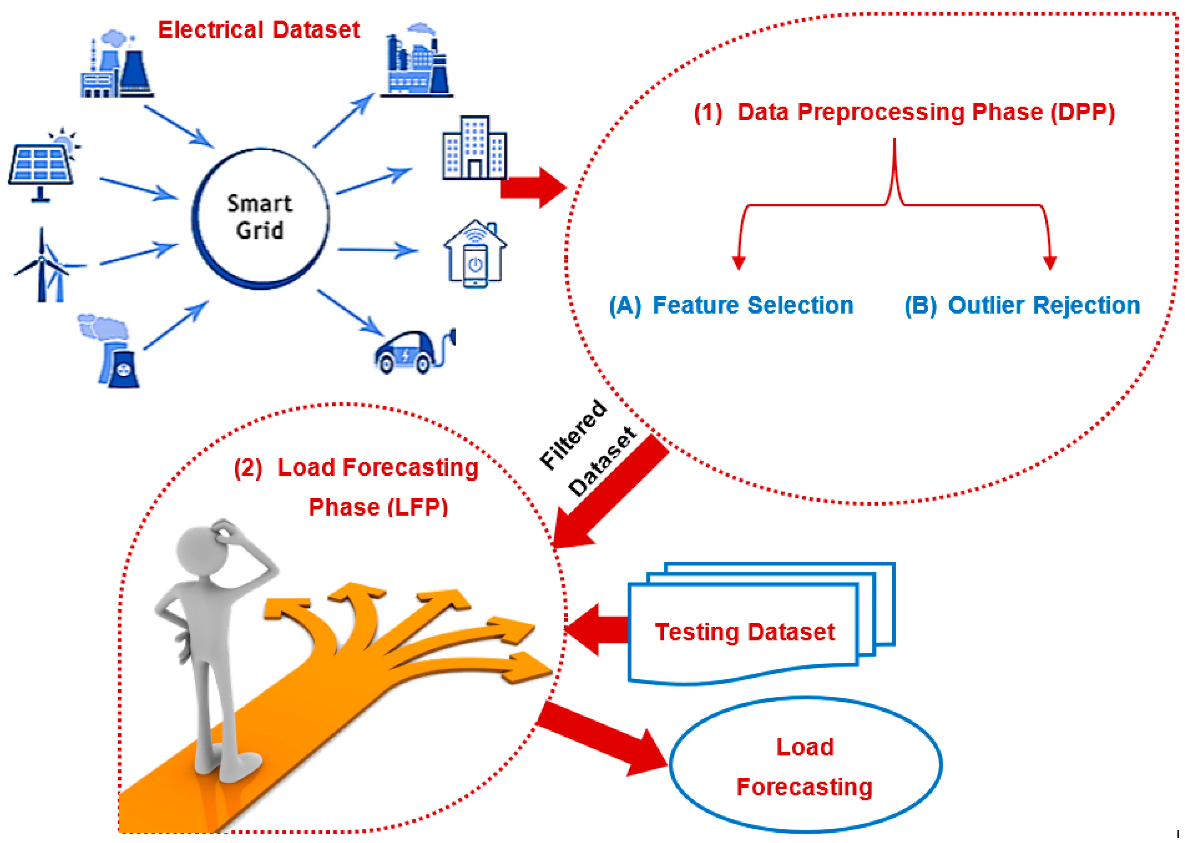
3. The Proposed Optimum Load Forecasting Strategy (OLFS)

In this section, the Optimum Load Forecasting Strategy (OLFS) as a new forecasting strategy is introduced to accurately estimate the amount of electricity required in the future. OLFS consists of two sequential phases called the Data Preprocessing Phase (DPP) and Load Forecasting Phase (LFP) as presented in Figure 1. DPP aims to filter irrelevant features and outliers from a dataset to obtain valid data. Then, LFP aims to provide a perfect load forecasting based on the valid dataset passed from DPP. In DPP, two main processes called feature selection and outlier rejection are applied to filter the electrical dataset before learning the load forecasting model in LFP to provide perfect results. While feature selection removes non-informative features, outlier rejection removes invalid items from the dataset to prevent overfitting problems and to enable the forecasting model to provide accurate results. At the end, the proposed load forecasting model in LFP is used to give perfect results. In this work, the feature selection process has been performed using a new selection method called Advanced Leopard Seal Optimization (ALSO). Then, Interquartile Range (IQR) was used to detect outliers. Finally, the Weighted K-Nearest Neighbor (WKNN) algorithm has been used to provide fast and accurate forecasts.

3.1. The Advanced Leopard Seal Optimization (ALSO)

In this subsection, a new feature selection method called Advanced Leopard Seal Optimization (ALSO) that combines both filter and wrapper approaches is discussed in detail. While filter approaches can quickly select a set of features, wrapper approaches can accurately select the best features. Hence, ALSO includes chi-square as a filter method [15] and Binary Leopard Seal Optimization (BLSO) as a wrapper method [16]. While chi-square is a fast but inaccurate method, BLSO is an accurate but slow method. Accordingly, ALSO contains both methods, so that each of them compensates for the problems of the other to determine the optimal set of features. The implementation of ALSO is represented in many steps as shown in Figure 2. At first, the collected dataset from smart electrical grids is subjected to chi-square to quickly select a set of informative features. Then, this set of features is subjected to BLSO to accurately select the most significant features in electrical load forecasting. BLSO begins with creating an initial population (P) including many leopard seals called search agents. It is assumed that P includes ‘n’ leopard seals (LS); LS = {LS₁, LS₂, ……, LS_n}. Each LS in P is represented in binary form where zero denotes a useless feature while one denotes a useful feature. After creating search agents in P, these agents are evaluated using the average accuracy value from ‘c’ classifiers as a fitness function to prove that the set of features selected can enable any classifier to give the best load forecasting. According to ‘c’ classifiers, the fitness function for the ith leopard seal (LS_i) can be measured by (1).

$$F\left({LS}_i\right)=\frac{\sum _{j=1}^c{A}_j\left({LS}_i\right)}{c}$$

(1)

where the fitness value for the ith leopard seal is F(LS_i), the classifier number that is used to calculate the fitness value of the selected features in each seal is c, and the accuracy of the jth classification according to the chosen features in the ith leopard seal is A_j(LS_i). To illustrate the idea, it is supposed that there are two seals in P, n = 2, and three classifiers, c = 3, applied to measure the fitness value of the selected features in every seal as illustrated in

Table 2. Identification of the best seal according to every classifier and average accuracy.

Classifier	Accuracy of Every Seal		The Best Seal
	LS1	LS2
C1 = SVM	0.75	0.75	LS2
C2 = KNN	0.9	0.8	LS1
C3 = NB	0.7	0.9	LS2
Average accuracy	0.767	0.816	LS2

. Related to Table 2, it is supposed that the applied classifiers are Support Vector Machine (SVM) [6,16], K-Nearest Neighbor (KNN) [4,17], and Naïve Bayes (NB) [4,5]. According to the accuracy of these classifiers, SVM and NB provide that the best seal is LS₂ while KNN provides that LS₁ is the best seal. Finally, the average accuracy value proved that the best seal is LS₂. Hence, evaluating seals based on a single classifier cannot give the best set of features that can enable any classifier to give the best results.

According to the fitness values, the highest fitness value indicates the best solution (seal) where the essential aim of the selection process is to provide the maximum average accuracy value. In fact, it is necessary to assign the iteration number (Y) and also the position vector number of the agents through its movement according to each iteration (£). Accordingly, the number of iterations for three phases called searching, encircling, and attacking based on the Y values have been calculated by (2)–(4) [2].

$$Y_{Sr}=⌊\frac{Y}{3}⌋$$

(2)

$$Y_{En}=⌊\frac{Y}{3}⌋$$

(3)

$$Y_{At}=\left(Y-2\ast ⌊\frac{Y}{3}⌋\right)$$

(4)

where Y_Sr, Y_En, and Y_At are the number of iterations for the searching, encircling, and attacking phases, respectively. To execute BLSO, the three phases have been sequentially implemented based on Y_Sr, Y_En, and Y_At as shown in Figure 2. Initially, the steps of the searching phase are executed until the iterations (Y_Sr) are terminated. In the case of the Y_Sr not being met, the position vectors of each agent are modified using (5).

$${\overrightarrow{ X}}_{\sigma }^j\left({LS}_u\right){|}_{\forall \sigma \{\mathrm{2,3},4,\dots ,\beta -1\}}={\overrightarrow{D}}^j\left({LS}_u\right).e^{b{f}_{\sigma }}\cos \left(2\pi f_{\sigma }\right)+{\overrightarrow{X}}_{\beta }^j\left({LS}_u\right)$$

(5)

where the modified $\sigma$’s position of LS_u at the jth iteration is ${\overrightarrow{X}}_{\sigma }^j\left({LS}_u\right)$, positions of LS_u from 2 to $\beta$ − 1 are $\sigma$, $\sigma${2, 3, 4,….,$\beta$ − 1}, and ${\overrightarrow{D}}^j\left({LS}_u\right)$ is the distance between the search agent and the prey that can be computed by (6). b is the logarithmic spiral shape, the angle scaling factor for the $\sigma$’s position of the agent is $f_{\sigma }$, computed by (7), and the modification of the last position ($\beta$’s position) of LS_u at the jth iteration is ${\overrightarrow{X}}_{\sigma }^j\left({LS}_u\right)$.

$${\overrightarrow{D}}^j\left({LS}_u\right)=\left|{\overrightarrow{X}}_{\beta }^j\left({LS}_u\right)-{\overrightarrow{X}}_1^j\left({LS}_u\right)\right|$$

(6)

$$f_{\sigma }=1-\frac{2\ast \sigma }{\beta }$$

(7)

where the modified 1st position of LS_u at the jth iteration is ${\overrightarrow{X}}_1^j\left({LS}_u\right)$, the total position number is β, and the current position of LS_u is $\sigma$. After updating the positions of agents, these new positions should be changed to a binary value by using a function called a sigmoid function (8) [16].

$${LS}_{b\_u}^i\left(\pounds +1\right)=\left\{\begin{array}{c}1 \mathrm{if} r\left(\mathrm{0,1}\right)\ge sig\left({LS}_u^i\right)\\ \\ 0 \mathrm{otherwise} \end{array}\right.$$

(8)

where ${LS}_{b\_u}^i\left(\pounds +1\right)$ is the binary value of the uth agent at the ith iteration in $\pounds +1$ that represents the next iteration, i = 1, 2, ..., f, and $sig\left({LS}_u^i\right)$ is the sigmoid function that has been calculated by (9) [15,16]. Furthermore, r(0, 1) is a random value between 0 and 1.

$$sig({LS}_u^i)=\frac{1}{1+e^{-L_u^i}}$$

(9)

where the base of the natural logarithm is e. In P, the new position of each seal ${LS}_{b\_u}^i\left(\pounds +1\right)$ has been evaluated by (1). Through searching for a prey, each agent in P will keep updated position and fitness values. In fact, the procedures of the searching phase are continued until the Y_Sr is terminated. Then, the best position in P for each agent is assigned based on the maximum evaluation value through their search for prey after the searching phase is completed. Related to the best agents in P generated by the searching phase, the steps of the encircling phase are implemented until the iterations (Y_En) are terminated. At first, the best leaders are determined based on the calculations of the evaluation function. Then, the Weighted Leaders Prey Allocation (WLPA) method is used for prey allocation [16]. The leopard seals update their positions depending on the prey’s position using (10)–(14).

$${\overrightarrow{D}}_{{LS}_u}^j=\left|\overrightarrow{C.}{\overrightarrow{X}}_{prey}^j-{\overrightarrow{X}}_{{LS}_u}^j\right|$$

(10)

$${\overrightarrow{X}}_{{LS}_u}^{j+1}={\overrightarrow{X}}_{prey}^j-\overrightarrow{A}.{\overrightarrow{D}}_{{LS}_u}^j$$

(11)

$$\overrightarrow{A}=2.\overrightarrow{a}.\overrightarrow{r_1}-\overrightarrow{a}$$

(12)

$$\overrightarrow{C}=2.\overrightarrow{r_2}$$

(13)

$$a=2-j\ast \frac{2}{Y_{En}}$$

(14)

where the uth agent’s position at iteration j is ${\overrightarrow{X}}_{{LS}_u}^j$, the forecasted position of the prey at the jth iteration is ${\overrightarrow{X}}_{prey}^j$, and the distance between the uth agent and the prey is ${\overrightarrow{D}}_{{LS}_u}^j$. Additionally, random vectors belonging to [0, 1] are $\overrightarrow{r_1}$ and $\overrightarrow{r_2}$, coefficient vectors are $\overrightarrow{A}$ and $\overrightarrow{C}$ calculated by (12) and (13), the number of iterations in the encircling phase is Y_En calculated by (3). A vector that decrements linearly from two to zero over the iterations is $\overrightarrow{a}$ computed by (14). In the encircling phase, the new position of a leopard seal is between the current position of the leopard seal and the prey’s position depending on $\overrightarrow{A}$ that includes a random value in [−1, 1]. If the Y_En is not met, leopard seals will update their positions based on the prey’s position by (10)–(14). At the end of the encircling phase, each leopard seal in P will be assigned its new position by calculating the distance between the leopard seal and prey by applying (10). After that, the new position of a leopard seal is calculated by applying (11) and then is evaluated using the evaluation (fitness) function for determining the best solutions (leaders). Then, the sigmoid function is applied to change all positions to be in binary form using (8).

The last phase, called the attacking phase, receives the last information from the previous encircling phase. Initially, the best leopard seals (alpha) are determined and their positions are used for determining the location of the target prey ${\overrightarrow{X}}_{prey}\left(\pounds \right)$. Then, the positions of leopard seals are converted into binary using the sigmoid function. If Y_At is not terminated, the leopard seals will modify their positions and then will test them by using the fitness function. At the end, the optimal solution is the fittest leopard seal that contains the best set of features.

3.2. Interquartile Range (IQR) Method

In this section, the Interquartile Range (IQR) method is used as an outlier rejection method to detect and then remove outliers. To use IQR, the dataset is divided into four equal parts or segments. To define the IQR, the distances between the quartiles are used. If a data point is more than 1.5 × IQR below the first segment or above the third segment, this data point is considered as an outlier. Multiplying the upper and lower IQR by 1.5 (1.5 × IQR) is a common method for detecting outliers where the value for controlling the sensitivity of the range is 1.5. Accordingly, all data points that are above Q3 + 1.5 × IQR and below Q1 − 1.5 × IQR are outliers, where Q3 is the third segment and Q1 is the first segment as shown in Figure 3. To calculate IQR, the first segment is subtracted from the third segment; IQR = Q3 − Q1.Then, IQR can be used to determine outliers by using many sequential steps: (i) the Interquartile Range (IQR) is calculated for the data, (ii) the Interquartile Range (IQR) is multiplied by 1.5, (iii) the maximum allowed normal value is determined; H = Q3 + 1.5 × (IQR). Accordingly, outliers are points that are greater than H, (vi) the minimum allowed normal value is determined; L = Q1 − 1.5 × (IQR). Accordingly, outliers are points that are lower than L.

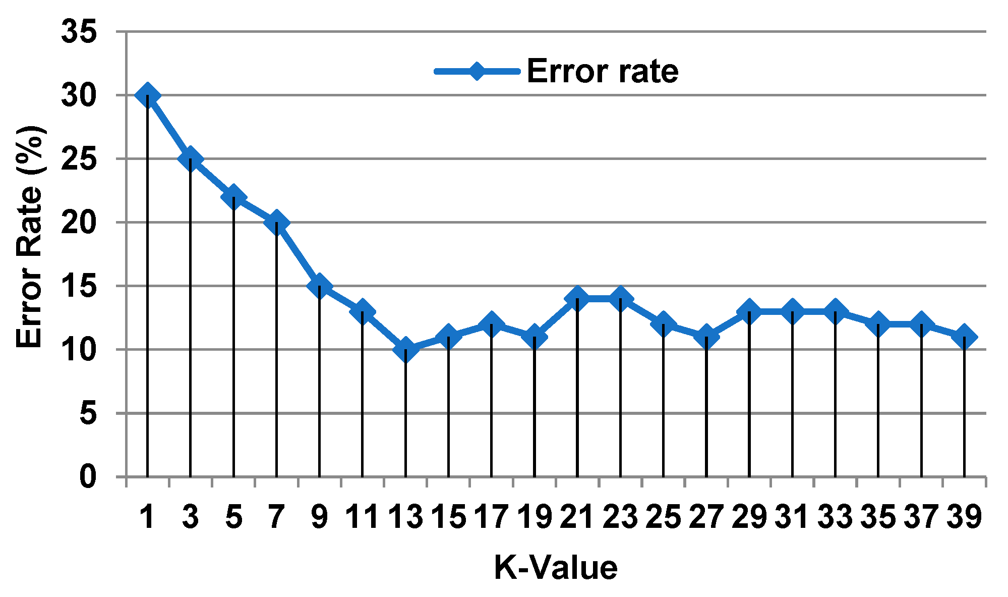
3.3. The Proposed Weighted K-Nearest Neighbor (WKNN) Algorithm

In this section, a new forecasting model called Weighted K-Nearest Neighbor (WKNN) is explained in detail. WKNN consists of two main methods called Naïve Bayes (NB) as a feature weighting method [6] and K-Nearest Neighbor (KNN) as a load forecasting method based on the weighted features [4,6]. In fact, the traditional KNN is a simple and straightforward method that can be easily implemented. On the other hand, KNN is based on measuring the distance between the features of each testing item and every training item separately without taking the impact of features on the class categories. Hence, NB is used as a weighting method to measure the impact of features on the class categories. Thus, a feature space is converted into a weight space. Then, KNN is implemented in weight space instead of feature space. In other words, the distance between any testing item and every training item is implemented in a weight space using the Euclidean distance [6].

Let a testing item be E = {$f_E^1$,$f_E^2$,….., $f_E^v$} and a training item be Q = {$f_Q^1$,$f_Q^2$,….., $f_Q^v$}, where $f_E^i$ is the ith feature value of the E testing item and $f_Q^i$ is the ith feature value of the Q training item; i = {1, 2, …, v}. Then, WKNN starts with calculating the Euclidean distance between each testing item in the testing dataset and every training item in the training dataset in v-dimension weight space using (15).

$$D\left(E, Q\right){|}_{class=c}=\sqrt{{\sum }_{i=1}^v{({{(f}_E^i)}^{\frac{1}{w_{cE}^{fi}}}-{{(f}_Q^i)}^{\frac{1}{w_{cQ}^{fi}}})}^2}$$

(15)

where $D\left(E, Q\right){|}_{class=c}$ is the Euclidean distance between E and Q items in class category c in a weight space. $w_{cE}^{fi}$ is the weight of the ith feature of the E item that belongs to c class while $w_{cE}^{fi}$ is the weight of the ith feature of the Q item that belongs to c class using (16).

$${ w}_{cE}^{fi}=P\left(cE|f_i\right)=P\left(cE\right).P\left(f_i|cE\right)$$

(16)

$$w_{cQ}^{fi}=P\left(cQ|f_i\right)=P\left(cQ\right).P\left(f_i|cQ\right)$$

(17)

where the probability that feature $f_i$ is in class $cE$ is $P\left(cE|f_i\right)$ and the probability that feature $f_i$ is in class $cQ$ is $P\left(cQ|f_i\right)$. Also, $P\left(cE\right)$ is the probability of the occurrence of class $cE$ and $P\left(cQ\right)$ is the probability of the occurrence of class $cQ$. $P\left(f_i|cE\right)$ is the probability of generating the feature $f_i$ given the class $cE$ and $P\left(f_i|cQ\right)$ is the probability of generating the feature $f_i$ given the class $cQ$. After calculating the distance (D) between each testing item and every training item separately using (15), distances should be in ascending order. Then, the k items that have the lowest distance values should be determined to take the average of their loads as a predicted load value for the testing or new item using (17).

$$Predicted\_Load (E)=\frac{\sum _{j=1}^{k}load\left(Q_j\right)}{k}$$

(18)

where $Predicted\_Load\left(E\right)$ is the predicted load of testing item $E$, $load\left(Q_j\right)$ is the load of the jth nearest training item, and k is the number of nearest neighbors. Figure 4 presents an example to illustrate the idea of implementing the WKNN algorithm.

4. Experimental Results

In this section, the proposed Optimum Load Forecasting Strategy (OLFS) that consists of two phases called the Data Preprocessing Phase (DPP) and Load Forecasting Phase (LFP) is executed. In DPP, the feature selection process using Advanced Leopard Seal Optimization (ALSO) and outlier rejection process using Interquartile Range (IQR) are implemented. Then, the filtered dataset is passed to the Weighted K-Nearest Neighbor (WKNN) algorithm in LFP to provide fast and accurate predictions. The proposed OLFS is implemented using an electricity load forecast dataset. Confusion matrix performance metrics are used to test the effectiveness of the proposed OLFS [4,6,16]. These metrics are accuracy, error, precision, and recall. Additionally, execution time is measured to test the speed of the proposed OLFS. The used parameters values are presented in

Table 3. The used parameter values in experiments.

Parameter	Description	Applied Value
b	A number that defines the movement shape of logarithmic spiral in the encircling phase	3
u	No. of alpha leopard seals	7
R	The maximum number of iterations	100
r	Random value that is needed in the sigmoid function	Random in [0, 1]
K	The number of nearest neighbors used in KNN method	1 ≤ K ≤ 40

. Actually, the K value is determined experimentally. To execute the KNN algorithm, many different values are applied using 1000 samples in the electricity load forecast dataset. The training dataset has 800 samples and the testing dataset has 200 samples. According to the K value, error value of KNN is assigned to find the optimal value of K that can give KNN the ability to introduce the minimum error values. In this work, the K value is between 1 and 40; K ∈ [1, 40]. The minimum error value is assigned at K = 13. Accordingly, the optimal value of K is 13 as shown in Figure 5. In the next experiments, the used value of K is 13.

4.1. Electricity Load Forecast Dataset Description

The electricity dataset is an internet dataset that consists of 16 features and 48,048 samples [17]. It is a short-term electricity load forecasting dataset that records data every hour. This dataset is from 3 January 2015 (01:00:00 a.m.) to 27 June 2020 (12:00:00 a.m.). The dataset contains historical electricity loads that are available in daily postdispatch reports and collected from the grid operator (CND). Additionally, this dataset includes calendar information that is related to school periods, from Panama’s Ministry of Education, and also includes calendar information that is related to holidays, from the ‘When on Earth?’ website. The dataset also includes weather variables such as relative humidity, temperature, wind speed, and precipitation. This dataset is divided into training and testing sets with 70% and 30% of the data, respectively. Hence, the training dataset includes 33,634 samples and the testing dataset includes 14.414 samples.

4.2. Testing the Proposed Optimum Load Forecasting Strategy (OLFS)

In this section, the proposed OLFS is tested against other load forecasting methods. These methods are GRU [1], HFM [2], ANN [3], SVR-RB [10], HPT [11], and LSTM [12] as presented in Table 1. Figure 6, Figure 7, Figure 8 and Figure 9 and

Table 4. The results of prediction methods at the maximum training sample number.

Prediction Methods	GRU	HFM	ANN	SVR-RB	HPT	LSTM	OLFS
Accuracy (%)	60	65	75	78	81	84	93
Error (%)	40	35	25	22	19	16	7
Precision (%)	58	60	64	69	74	79	82
Recall (%)	80	55	59	63	68	73	75
Implementation time (s)	7.88	7.5	7	6.6	6	5.7	5.1

illustrate the accuracy, error, precision, and recall of OLFS against other load forecasting methods. Additionally, Figure 10 and Table 4 show the execution time of OLFS against other load forecasting methods. Figure 6, Figure 7, Figure 8, Figure 9 and Figure 10 and Table 4 show that OLFS can provide accurate results in the minimum execution time.

Figure 6, Figure 7, Figure 8 and Figure 9 and Table 4 show that OLFS provides the maximum accuracy, precision, and recall values and it provides the minimum error and execution time values according to the number of training samples. Related to Figure 6 and Table 4, the accuracies of GRU, HFM, ANN, SVR-RB, HPT, LSTM, and OLFS are 60%, 65%, 75%, 78%, 81%, 84%, and 93%, respectively, at the maximum training sample number. Figure 7 and Table 4 show that the errors of GRU, HFM, ANN, SVR-RB, HPT, LSTM, and OLFS are 40%, 35%, 25%, 22%, 19%, 16%, and 7%s respectively, at the maximum training sample number. Accordingly, OLFS provides the best accuracy and error values while GRU provides the worst values. According to Figure 8 and Table 4, the precisions of GRU, HFM, ANN, SVR-RB, HPT, LSTM, and OLFS are 58%, 60%, 64%, 69%, 74%, 79%, and 82%, respectively, at the maximum training sample number. Hence, the maximum precision value is provided by OLFS and the minimum value is provided by GRU.

Figure 9 and Table 4 illustrate that the recall of OLFS is better than that of GRU, HFM, ANN, SVR-RB, HPT, and LSTM with values of 80%, 55%, 59%, 63%, 68%, 73%, and 75%, respectively, at the maximum training sample number. According to Figure 10 and Table 4, the minimum execution time is provided by OLFS and the maximum execution time is provided by GRU with values of 5.1 s and 7.88 s, respectively, at the maximum training sample number. The execution times of HFM, ANN, SVR-RB, HPT, and LSTM are 7.5, 7, 6.6, 6, and 5.7 s, respectively, at the maximum training sample number. Thus, Figure 6, Figure 7, Figure 8, Figure 9 and Figure 10 and Table 4 proved that the proposed OLFS can provide the best results compared to other load forecasting methods (GRU, HFM, ANN, SVR-RB, HPT, and LSTM). From these results, it is noted that OLFS outperforms the other methods (GRU, HFM, ANN, SVR-RB, HPT, and LSTM) as it depended on using two main processes, feature selection and outlier rejection, before using the prediction model. Hence, the prediction model has accurately been learned based on the filtered dataset.

5. Conclusions and Future Works

In this paper, a new load forecasting strategy called the Optimum Load Forecasting Strategy (OLFS) has been introduced to provide fast and accurate results. OLFS consists of two phases called the Data Preprocessing Phase (DPP) and Load Forecasting Phase (LFP). Two main processes called feature selection and outlier rejection have been used in DPP to prepare and filter irrelevant features and outliers from the dataset. Feature selection has been performed using Advanced Leopard Seal Optimization (ALSO) while outlier rejection has been performed using Interquartile Range (IQR). Next, the Weighted K-Nearest Neighbor (WKNN) algorithm has been used as load forecasting method in LFP based on the prepared dataset to quickly provide accurate results. Experimental results showed that the proposed OLFS provides the maximum accuracy, precision, and recall values but the minimum error and execution time with values equal to 93%, 82%, 80%, 7%, and 5.1 s, respectively, at the maximum training sample number. Finally, the proposed OLFS can provide fast and accurate predictions. In the future, a new outlier rejection method using an optimization algorithm such as the red piranha optimization algorithm will be used to provide more accurate predictions. Additionally, a classification model based on a deep learning algorithm will be applied to enhance the results.

References

1. Abumohsen, M.; Owda, A.; Owda, M. Electrical Load Forecasting Using LSTM, GRU, and RNN Algorithms. Energies 2023, 16, 2283. [Google Scholar] [CrossRef]
2. Gomez, W.; Wang, F.; Amogne, Z. Electricity Load and Price Forecasting Using a Hybrid Method Based Bidirectional Long Short-Term Memory with Attention Mechanism Model. Int. J. Energy Res. 2023, 2023, 1–18. [Google Scholar] [CrossRef]
3. Tarmanini, C.; Sarma, N.; Gezegin, C.; Ozgonenel, O. Short term load forecasting based on ARIMA and ANN approaches. Energy Rep. 2023, 9, 550–557. [Google Scholar] [CrossRef]
4. Rabie, A.H.; Ali, S.H.; Saleh, A.I.; Ali, H.A. A fog based load forecasting strategy based on multi-ensemble classification for smart grids. J. Ambient. Intell. Humaniz. Comput. 2020, 11, 209–236. [Google Scholar] [CrossRef]
5. Rabie, A.; Saleh, A.; Ali, H. Smart electrical grids based on cloud, IoT, and big data technologies: State of the art. J. Ambient. Intell. Humaniz. Comput. 2021, 12, 9450–9478. [Google Scholar] [CrossRef]
6. Saleh, A.I.; Rabie, A.H.; Abo-Al-Ez, K.M. A data mining based load forecasting strategy for smart electrical grids. Adv. Eng. Inform. 2016, 30, 422–448. [Google Scholar] [CrossRef]
7. Tian, M.-W.; Alattas, K.; El-Sousy, F.; Alanazi, A.; Mohammadzadeh, A.; Tavoosi, J.; Mobayen, S.; Skruch, P. A New Short Term Electrical Load Forecasting by Type-2 Fuzzy Neural Networks. Energies 2022, 15, 3034. [Google Scholar] [CrossRef]
8. Mounir, N.; Ouadi, H.; Jrhilifa, I. Short-term electric load forecasting using an EMD-BI-LSTM approach for smart grid energy management system. Energy Build. 2023, 288, 113022. [Google Scholar] [CrossRef]
9. Lin, F.-J.; Chang, C.-F.; Huang, Y.-C.; Su, T.-M. A Deep Reinforcement Learning Method for Economic Power Dispatch of Microgrid in OPAL-RT Environment. Technologies 2023, 11, 96. [Google Scholar] [CrossRef]
10. Alrashidi, A.; Qamar, A.M. Data-Driven Load Forecasting Using Machine Learning and Meteorological Data. Comput. Syst. Sci. Eng. 2022, 44, 1973–1988. [Google Scholar] [CrossRef]
11. Khan, S. Short-Term Electricity Load Forecasting Using a New Intelligence-Based Application. Sustainability 2023, 15, 12311. [Google Scholar] [CrossRef]
12. Cordeiro-Costas, M.; Villanueva, D.; Eguía-Oller, P.; Martínez-Comesaña, M.; Ramos, S. Load Forecasting with Machine Learning and Deep Learning Methods. Appl. Sci. 2023, 13, 7933. [Google Scholar] [CrossRef]
13. Chodakowska, E.; Nazarko, J.; Nazarko, Ł. ARIMA Models in Electrical Load Forecasting and Their Robustness to Noise. Energies 2021, 14, 7952. [Google Scholar] [CrossRef]
14. Wang, A.; Yu, Q.; Wang, J.; Yu, X.; Wang, Z.; Hu, Z. Electric Load Forecasting Based on Deep Ensemble Learning. Appl. Sci. 2023, 13, 9706. [Google Scholar] [CrossRef]
15. Janane, F.Z.; Ouaderhman, T.; Chamlal, H. A filter feature selection for high-dimensional data. J. Algorithms Comput. Technol. 2023, 17, 17483026231184171. [Google Scholar] [CrossRef]
16. Nicholas, P.; Tayaza, F.; Andreas, W.; Justin, M. A Review of Feature Selection Methods for Machine Learning-Based Disease Risk Prediction. Front. Bioinform. 2022, 2, 927312. [Google Scholar]
17. Available online: https://www.kaggle.com/datasets/saurabhshahane/electricity-load-forecasting (accessed on 1 December 2023).
Figure 1. The main steps of the proposed Optimum Load Forecasting Strategy (OLFS).
Technologies 12 00019 g001
Figure 2. Steps of implementing the ALSO.
Technologies 12 00019 g002
Figure 3. The boxplot that represents the Interquartile Range (IQR) method as an outlier rejection method.
Technologies 12 00019 g003
Figure 4. Load forecasting using WKNN algorithm. 1: Feature Space; 2: Weight Spaces; 3: Load Forecasting.
Technologies 12 00019 g004
Figure 5. Error rate vs. K value.
Technologies 12 00019 g005
Figure 6. Accuracy of load forecasting methods.
Technologies 12 00019 g006
Figure 7. Error of load forecasting methods.
Technologies 12 00019 g007
Figure 8. Precision of load forecasting methods.
Technologies 12 00019 g008
Figure 9. Recall of load forecasting methods.
Technologies 12 00019 g009
Figure 10. Execution time of load forecasting methods.
Technologies 12 00019 g010