


A New LCL Filter Design Method for Single-Phase Photovoltaic Systems Connected to the Grid via Micro-Inverters

 ,
,  , ,
, ,  ,
,
Abstract
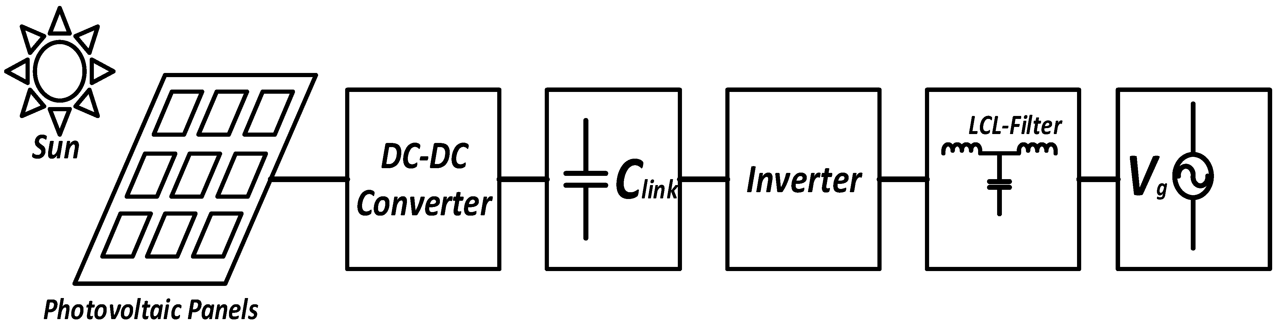
:1. Introduction
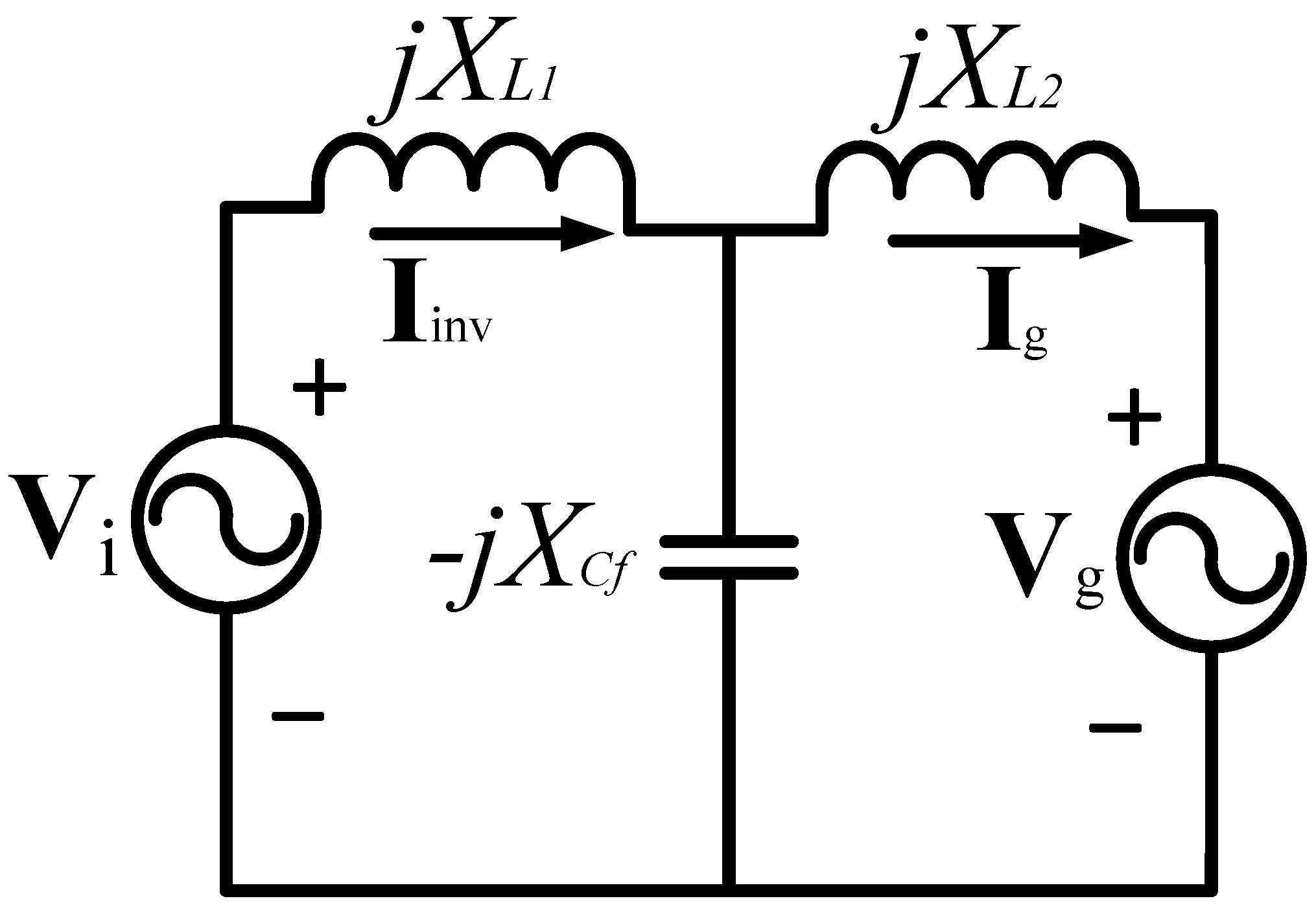
2. LCL Filter Mathematical Analysis
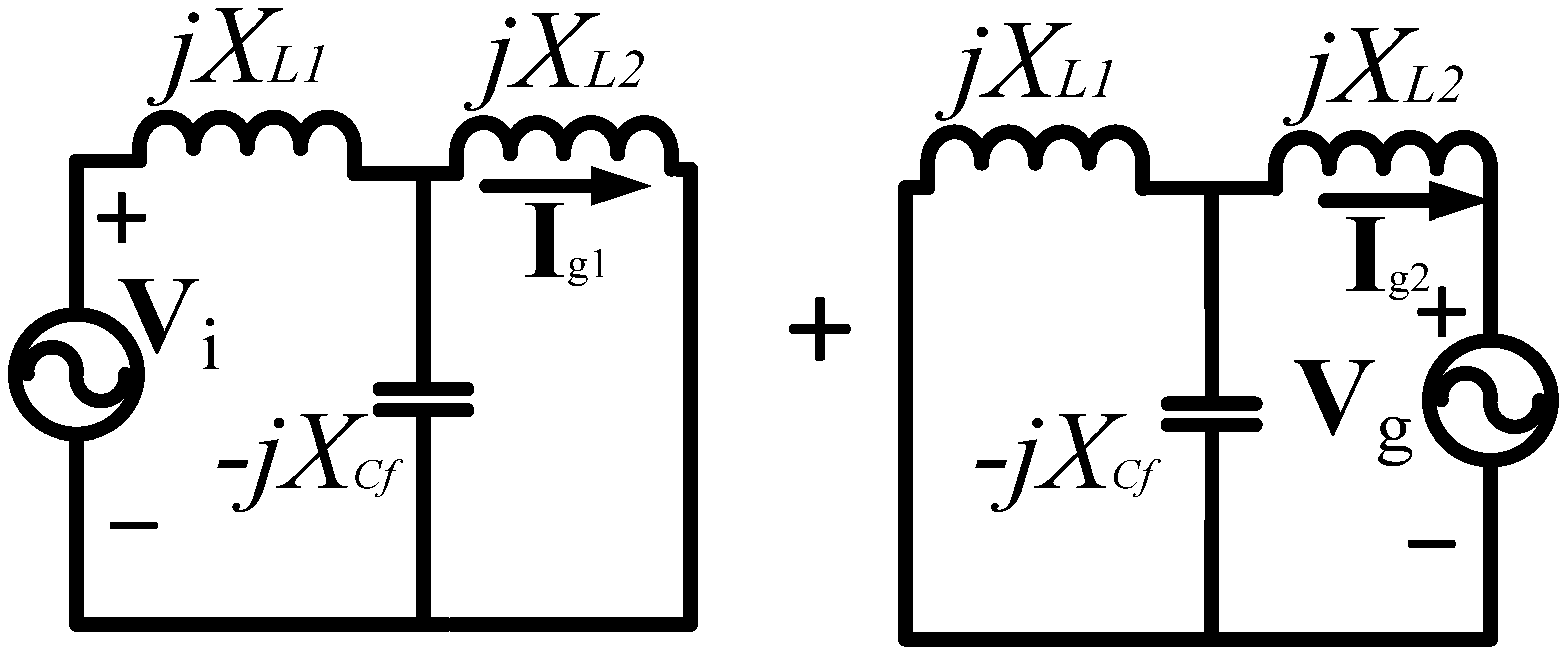
2.1. Mathematical Analysis of the LCL Filter for the Fundamental Component
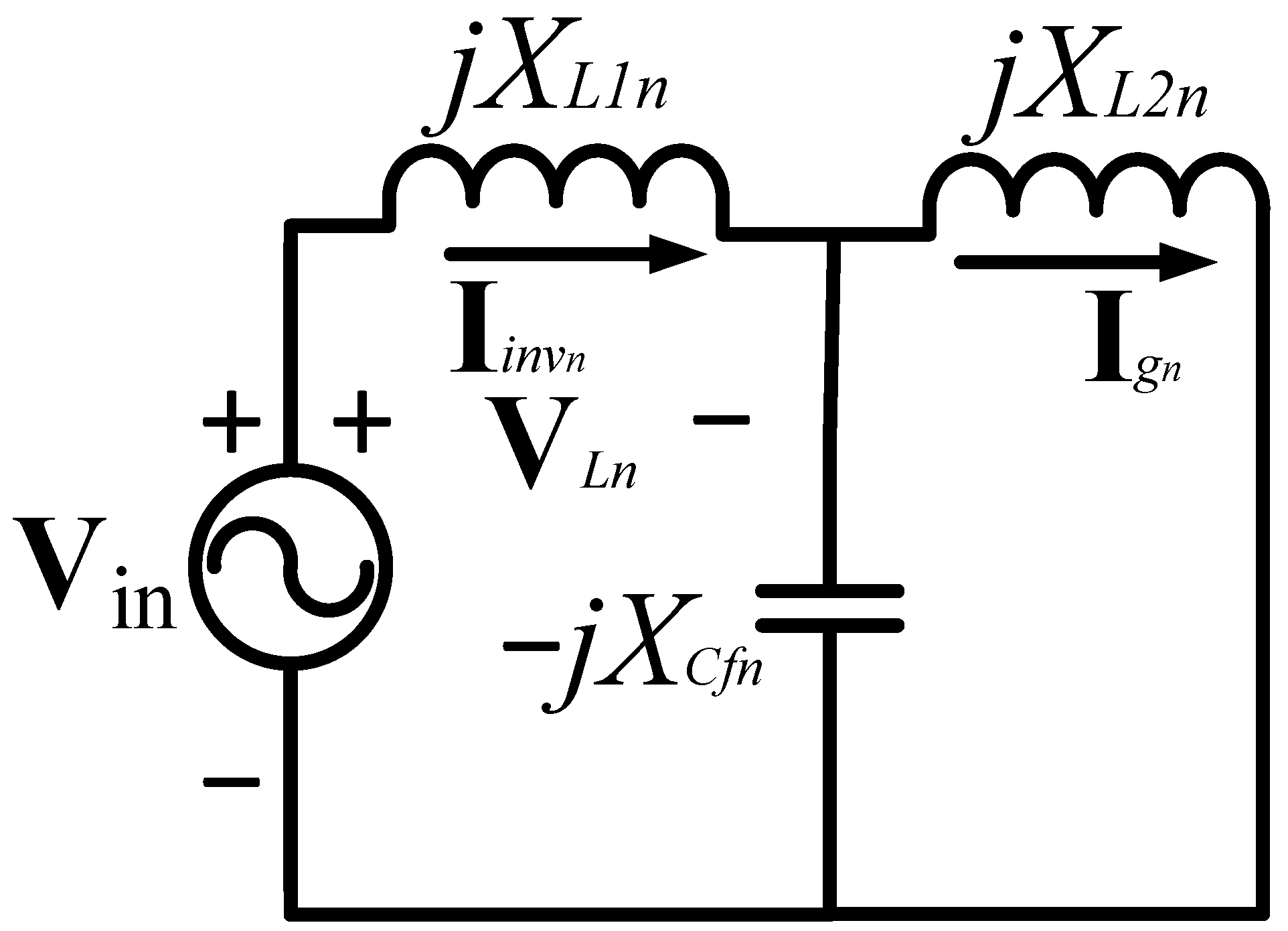
2.2. Mathematical Analysis of the LCL Filter for a Harmonic n
2.3. Mathematical Analysis to Calculate LCL Filter Elements
2.4. Resonance Frequency
2.5. DC Bus Calculation
2.6. Attenuation Coefficient to Determine Beta
3. Design and Optimization of an LCL Filter Connected to the Grid
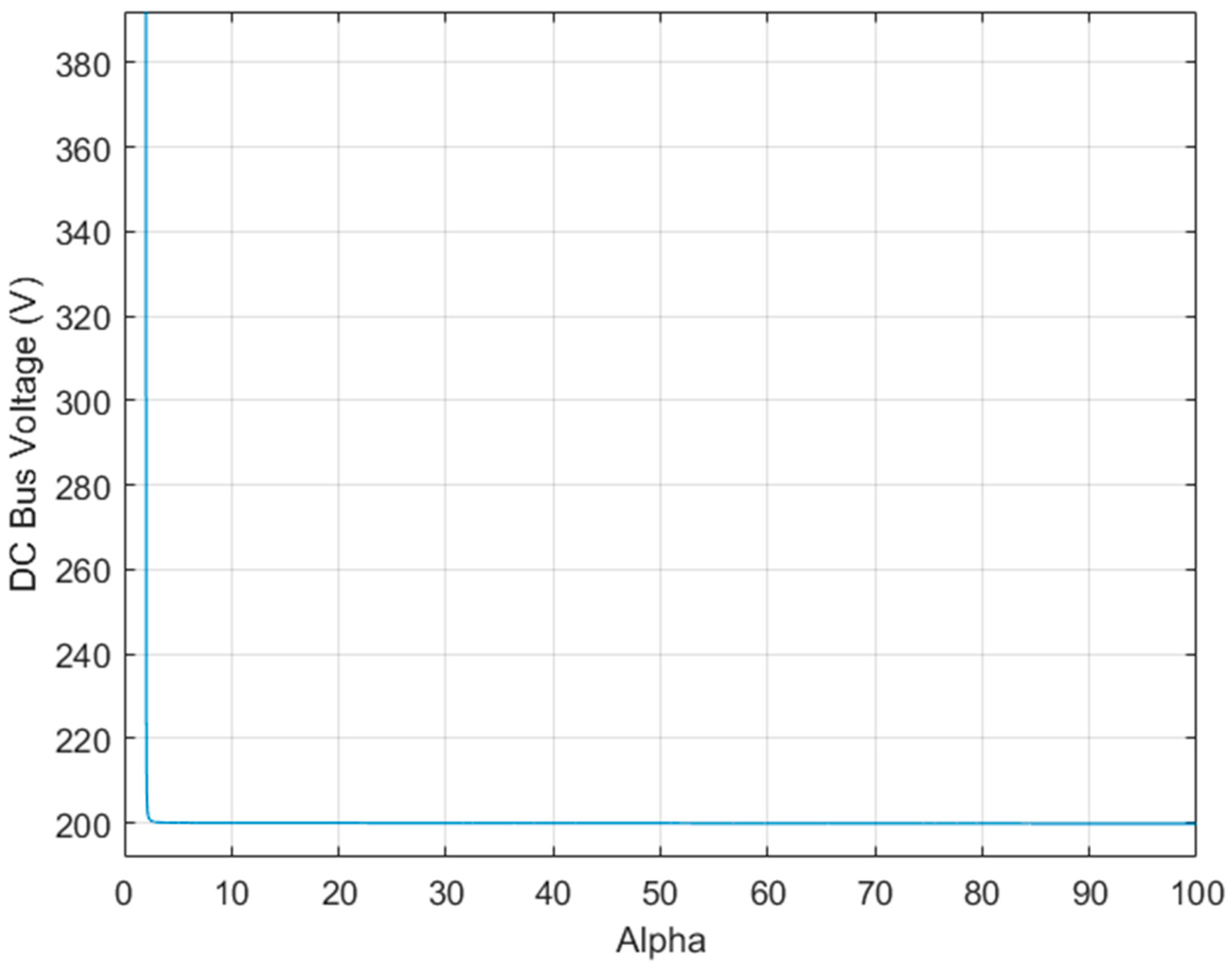
3.1. Step 1. Vdc Calculation
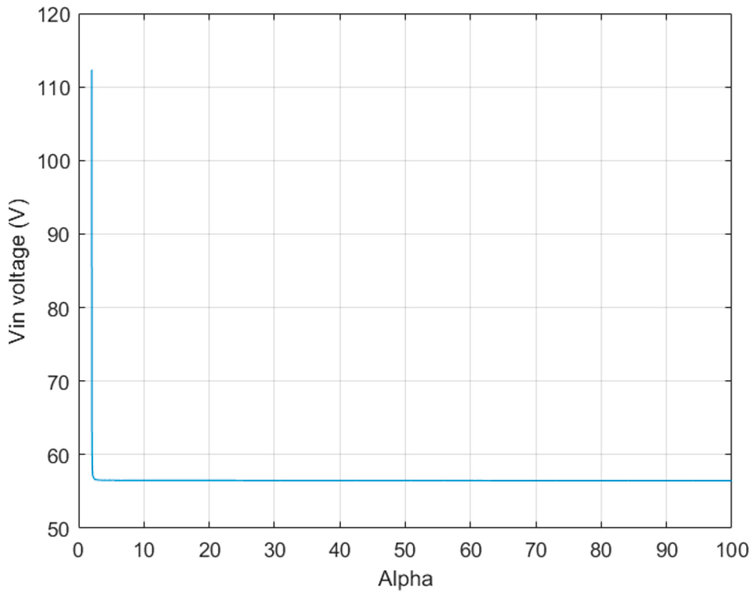
3.2. Step 2. Vin Calculation
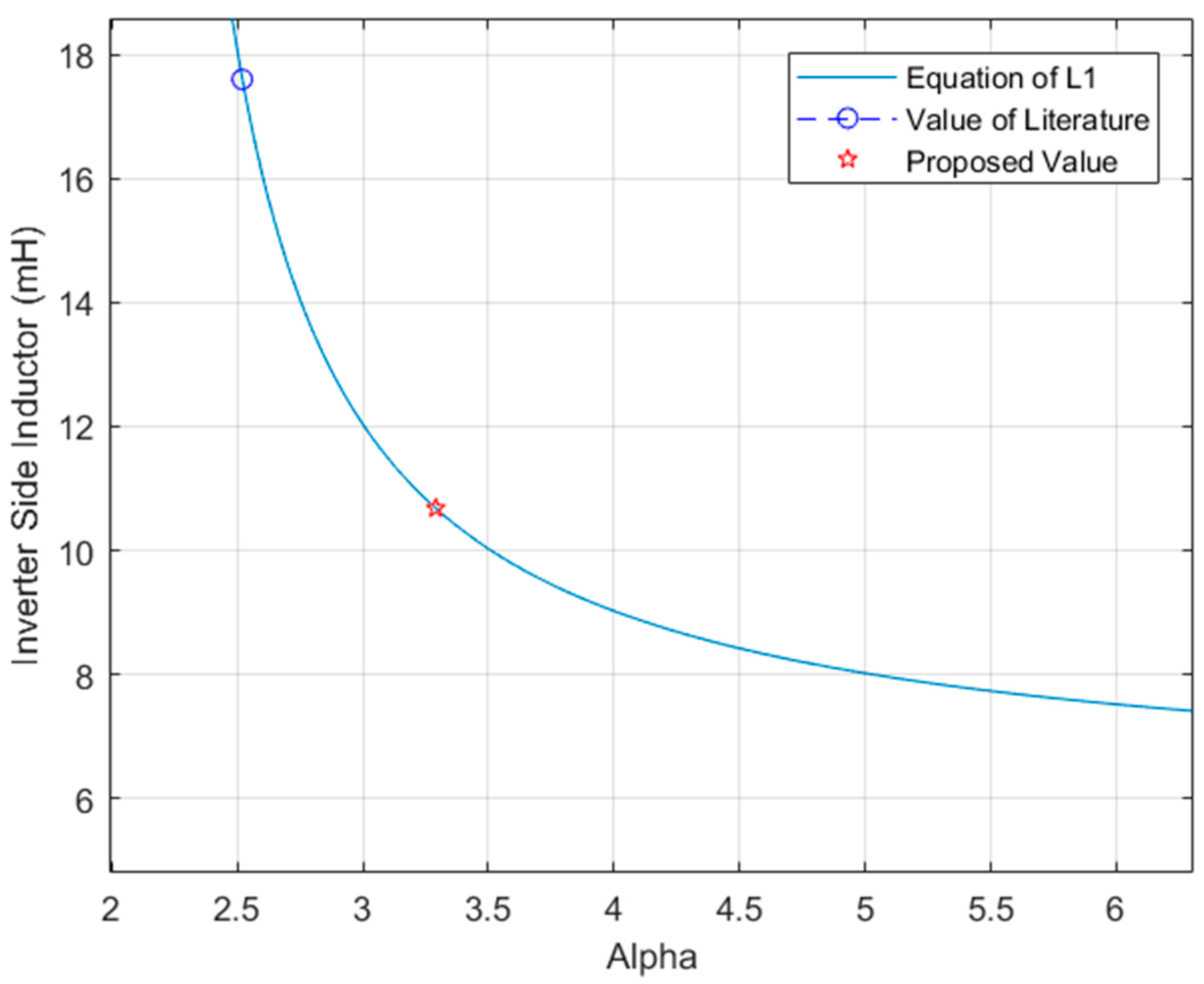
3.3. Step 3. Inductance L1 Calculation
3.4. Step 4. Inductance L2 Calculation
3.5. Step 5. LCL Filter Capacitor Calculation (Cf)
3.6. Step 6. Resonance Frequency Calculation (fr)
3.7. Step 7. Calculation of Link Capacitor (Cf)
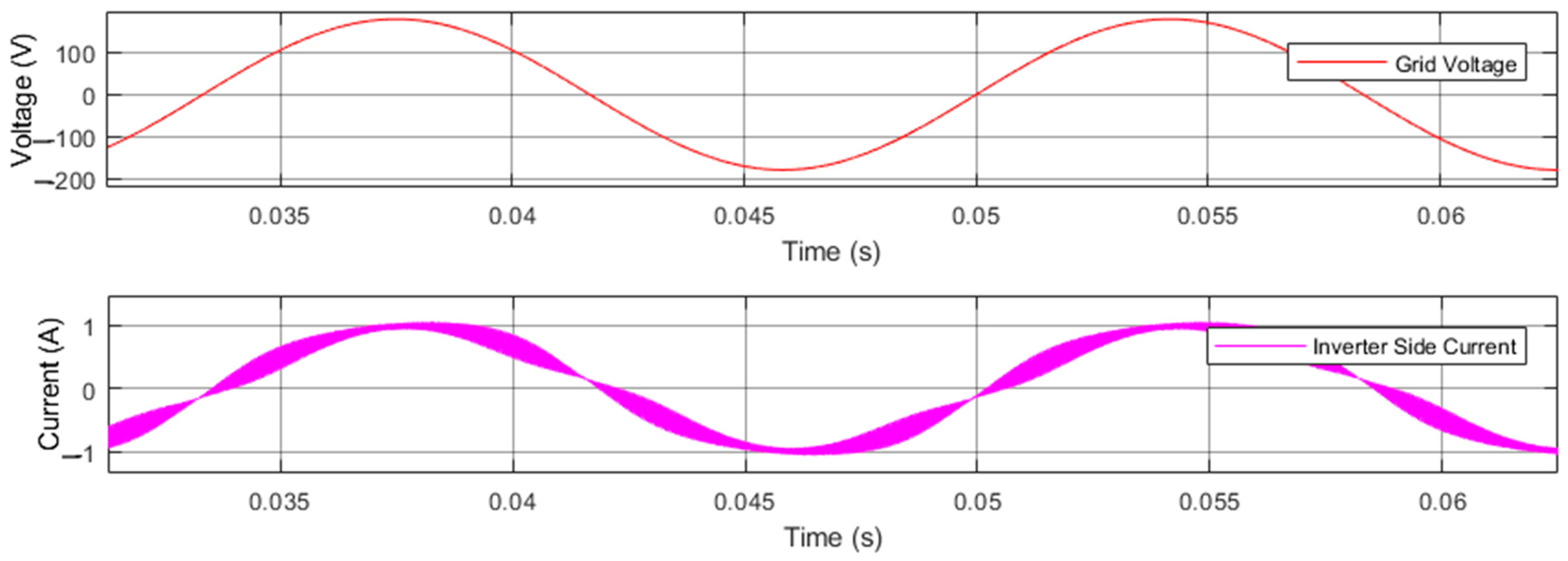
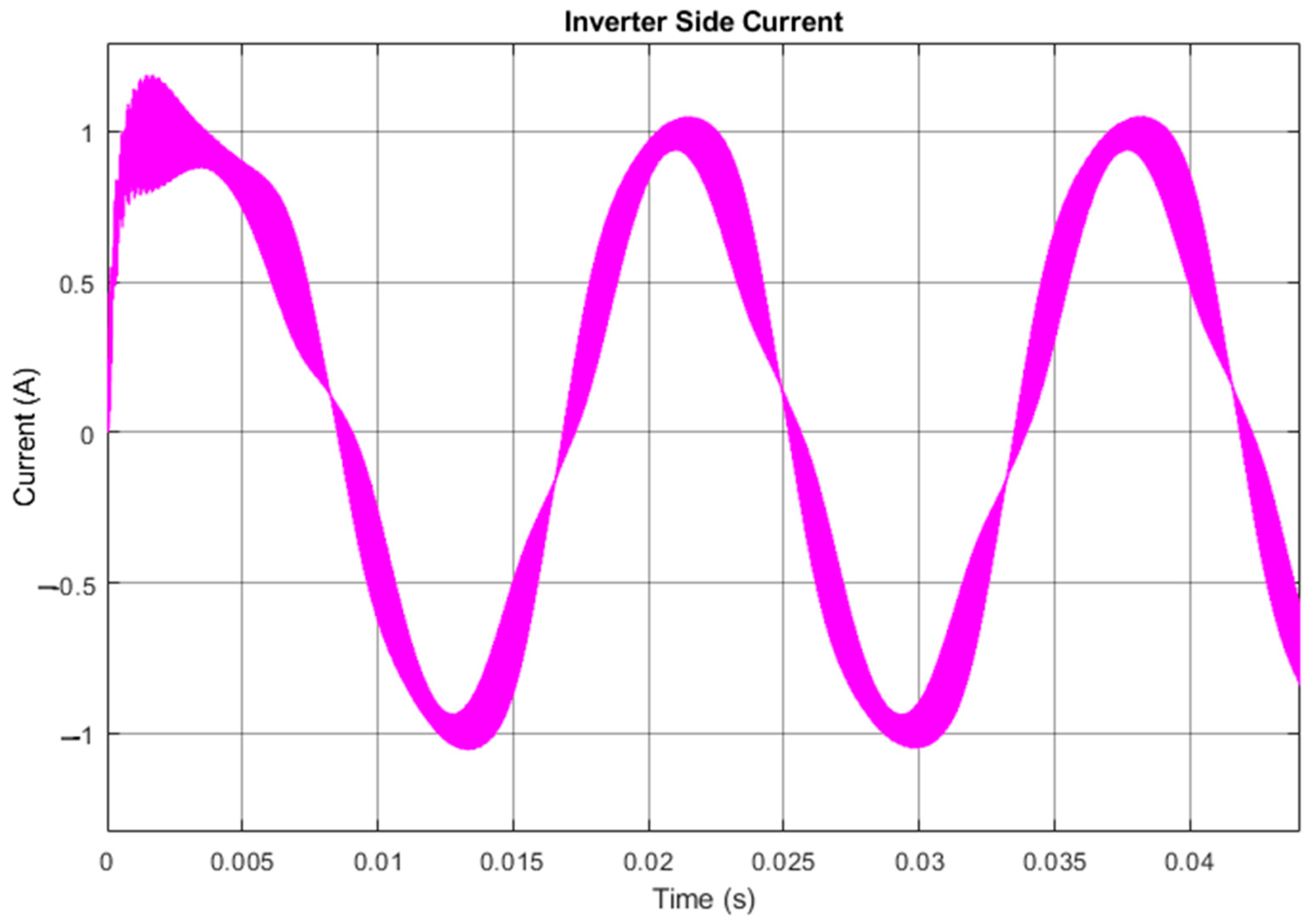
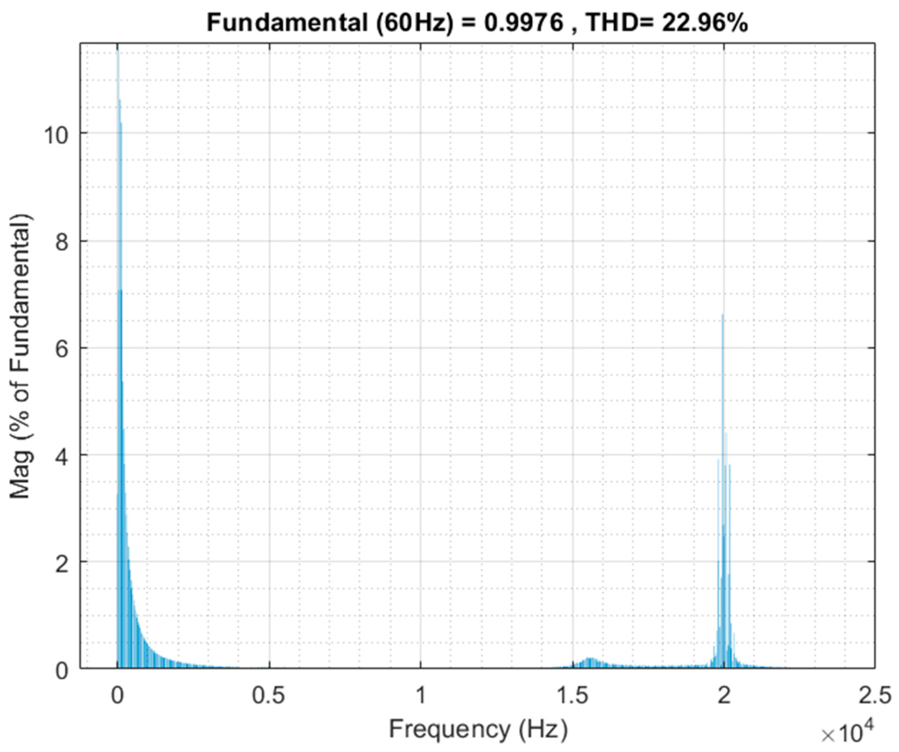
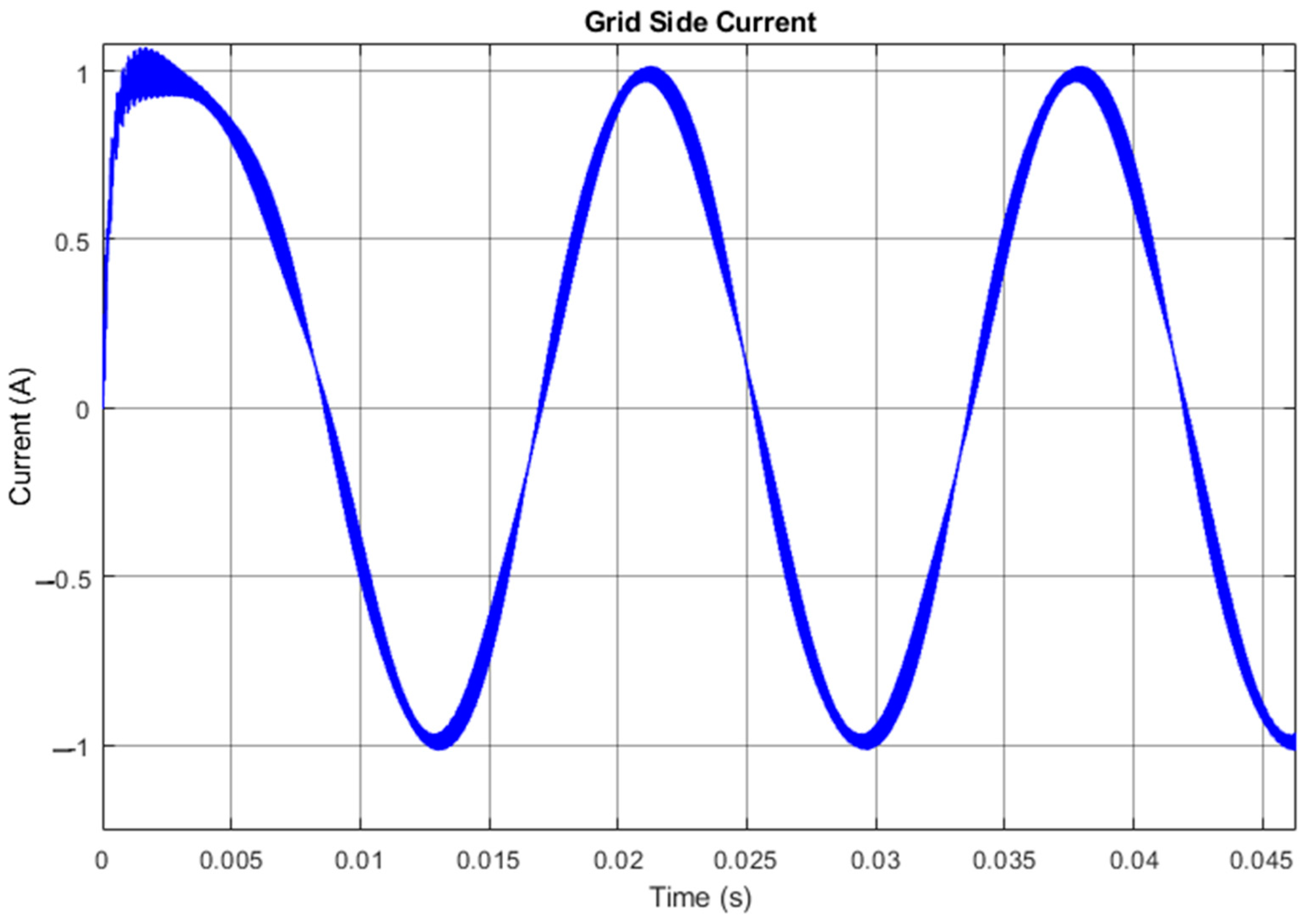
4. Simulation Results
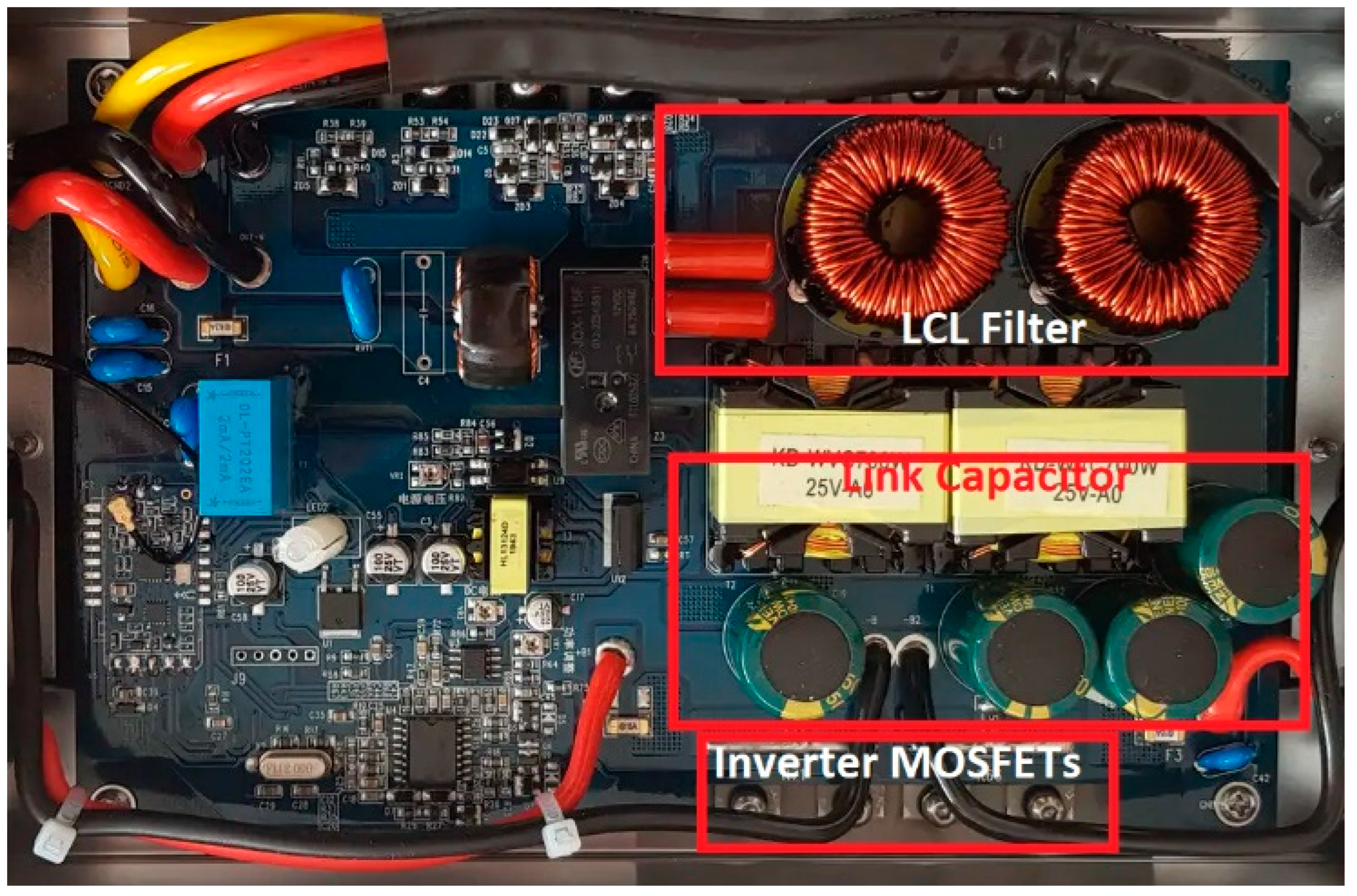
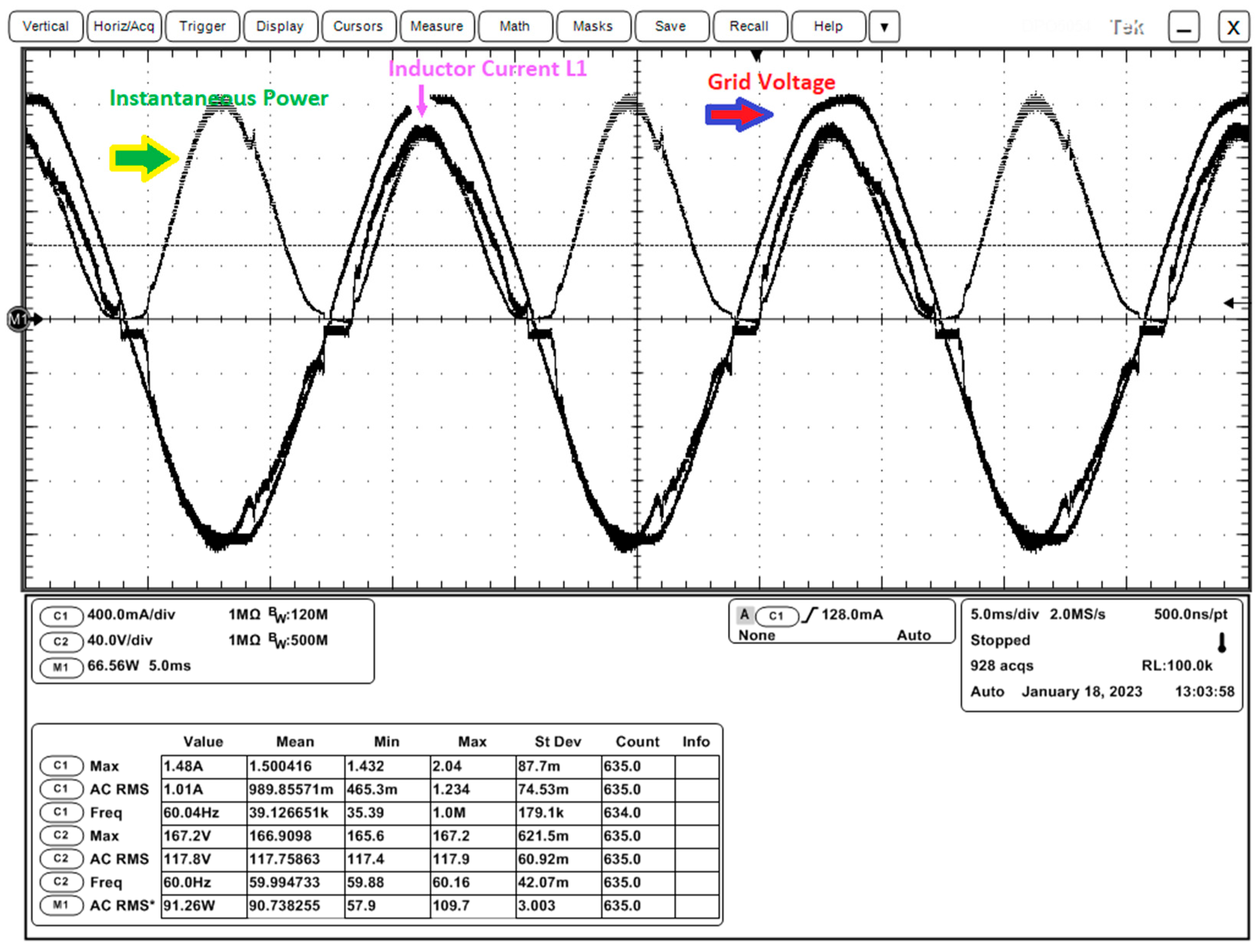
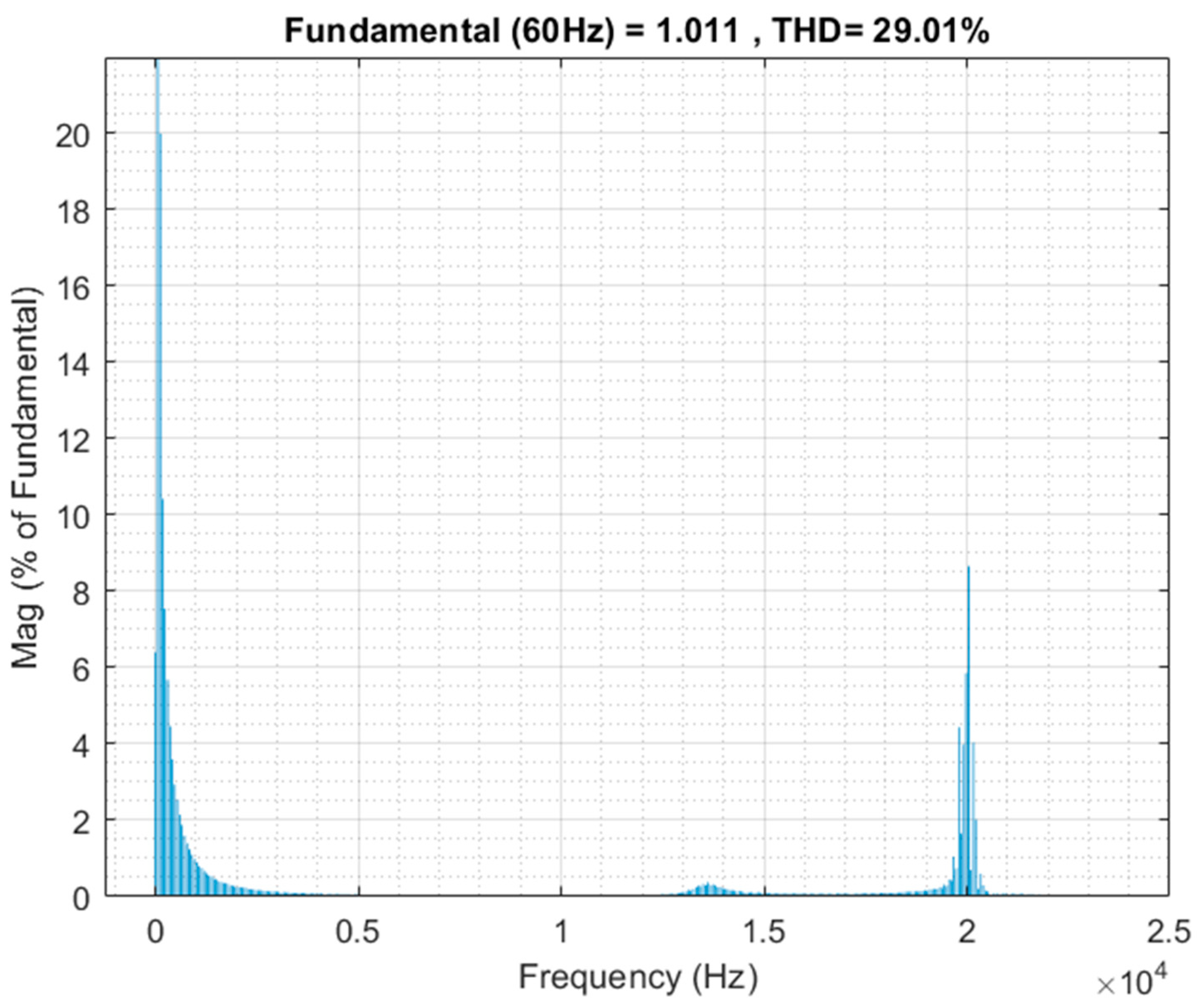
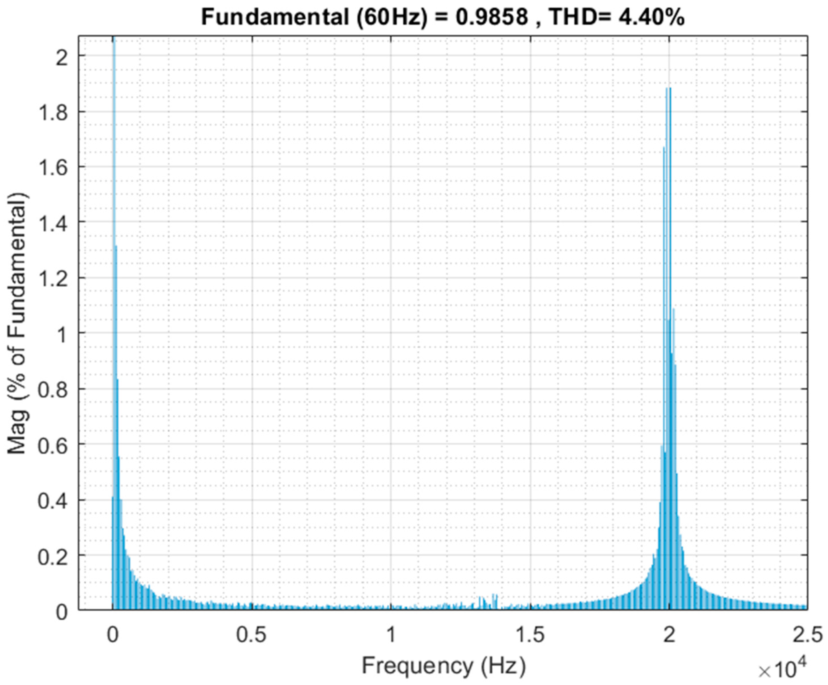
5. Experimental Results
6. Discussion
7. Conclusions
Author Contributions
Funding
Data Availability Statement
Conflicts of Interest
References
- Lai, C.S.; Jia, Y.; Lai, L.L.; Xu, Z.; McCulloch, M.D.; Wong, K.P. A comprehensive review on large-scale photovoltaic system with applications of electrical energy storage. Renew. Sustain. Energy Rev. 2017, 78, 439–451. [Google Scholar] [CrossRef]
- Chatterjee, S.; Kumar, P.; Chatterjee, S. A techno-commercial review on grid connected photovoltaic system. Renew. Sustain. Energy Rev. 2018, 81, 2371–2397. [Google Scholar] [CrossRef]
- Kabir, E.; Kumar, P.; Kumar, S.; Adelodun, A.A.; Kim, K.-H. Solar energy: Potential and future prospects. Renew. Sustain. Energy Rev. 2018, 82, 894–900. [Google Scholar] [CrossRef]
- Adamas-Pérez, H.; Ponce-Silva, M.; Mina-Antonio, J.D.; Claudio-Sánchez, A.; Rodríguez-Benítez, O. Assessment of Energy Conversion in Passive Components of Single-Phase Photovoltaic Systems Interconnected to the Grid. Electronics 2023, 12, 3341. [Google Scholar] [CrossRef]
- Ghosh, S.; Yadav, R. Future of photovoltaic technologies: A comprehensive review. Sustain. Energy Technol. Assess. 2021, 47, 101410. [Google Scholar] [CrossRef]
- Marques Lameirinhas, R.A.; Torres, J.P.N.; de Melo Cunha, J.P. A photovoltaic technology review: History, fundamentals and applications. Energies 2022, 15, 1823. [Google Scholar] [CrossRef]
- Rodríguez-Benítez, O.; Ponce-Silva, M.; Aqui-Tapia, J.A.; Rodríguez-Benítez, Ó.M.; Lozoya-Ponce, R.E.; Adamas-Pérez, H. Active Power-Decoupling Methods for Photovoltaic-Connected Applications: An Overview. Processes 2023, 11, 1808. [Google Scholar] [CrossRef]
- Rasekh, N.; Hosseinpour, M. LCL filter design and robust converter side current feedback control for grid-connected Proton Exchange Membrane Fuel Cell system. Int. J. Hydrogen Energy 2020, 45, 13055–13067. [Google Scholar] [CrossRef]
- Sedo, J.; Kascak, S. Design of output LCL filter and control of single-phase inverter for grid-connected system. Electr. Eng. 2017, 99, 1217–1232. [Google Scholar] [CrossRef]
- Ruan, X.; Wang, X.; Pan, D.; Yang, D.; Li, W.; Bao, C. Control Techniques for LCL-Type Grid-Connected Inverters; Springer: Singapore, 2018. [Google Scholar]
- Ibrahim, N.F.; Mahmoud, M.M.; Al Thaiban, A.M.; Barnawi, A.B.; Elbarbary, Z.S.; Omar, A.I.; Abdelfattah, H. Operation of grid-connected PV system with ANN-based MPPT and an optimized LCL filter using GRG algorithm for enhanced power quality. IEEE Access 2023, 11, 106859–106876. [Google Scholar] [CrossRef]
- Cai, Y.; He, Y.; Zhou, H.; Liu, J. Design method of LCL filter for grid-connected inverter based on particle swarm optimization and screening method. IEEE Trans. Power Electron. 2021, 36, 10097–10113. [Google Scholar] [CrossRef]
- Cittanti, D.; Mandrile, F.; Gregorio, M.; Bojoi, R. Design Space Optimization of a Three-Phase LCL Filter for Electric Vehicle Ultra-Fast Battery Charging. Energies 2021, 14, 1303. [Google Scholar] [CrossRef]
- Osório, C.R.; Schuetz, D.A.; Koch, G.G.; Carnielutti, F.; Lima, D.M.; Maccari Jr, L.A.; Montagner, V.F.; Pinheiro, H. Modulated model predictive control applied to lcl-filtered grid-tied inverters: A convex optimization approach. IEEE Open J. Ind. Appl. 2021, 2, 366–377. [Google Scholar] [CrossRef]
- Park, K.-B.; Kieferndorf, F.D.; Drofenik, U.; Pettersson, S.; Canales, F. Optimization of LCL filter with integrated intercell transformer for two-interleaved high-power grid-tied converters. IEEE Trans. Power Electron. 2019, 35, 2317–2333. [Google Scholar] [CrossRef]
- Hasan, F.A.; Rashad, L.J.; Humod, A.T. Integrating Particle Swarm Optimization and Routh-Hurwitz’s Theory for Controlling Grid-Connected LCL-Filter Converter. Int. J. Intell. Eng. Syst. 2020, 13, 102–113. [Google Scholar] [CrossRef]
- Gurrola-Corral, C.; Segundo, J.; Esparza, M.; Cruz, R. Optimal LCL-filter design method for grid-connected renewable energy sources. Int. J. Electr. Power Energy Syst. 2020, 120, 105998. [Google Scholar] [CrossRef]
- Long, B.; Zhu, Z.; Yang, W.; Chong, K.T.; Rodríguez, J.; Guerrero, J.M. Gradient descent optimization based parameter identification for FCS-MPC control of LCL-type grid connected converter. IEEE Trans. Ind. Electron. 2021, 69, 2631–2643. [Google Scholar] [CrossRef]
- Hernandez, O.; Mina, J.; Calleja, J.H.; Pérez, A.C.; de Leon, S.E. A multi-objective optimized design of LCL filters for grid-connected voltage source inverters considering discrete components. Int. Trans. Electr. Energy Syst. 2021, 31, e12908. [Google Scholar] [CrossRef]
- Azab, M. Multi-objective design approach of passive filters for single-phase distributed energy grid integration systems using particle swarm optimization. Energy Rep. 2020, 6, 157–172. [Google Scholar] [CrossRef]
- Khan, D.; Qais, M.; Sami, I.; Hu, P.; Zhu, K.; Abdelaziz, A.Y. Optimal Lcl-Filter Design for a Single-Phase Grid-Connected Inverter Using Metaheuristic Algorithms. Comput. Electr. Eng. 2023, 110, 108857. [Google Scholar] [CrossRef]
- Khan, M.A.; Haque, A.; Kurukuru, V.S.B.; Blaabjerg, F. Optimizing the Performance of Single-Phase Photovoltaic Inverter using Wavelet-Fuzzy Controller. e-Prime-Adv. Electr. Eng. Electron. Energy 2023, 3, 100093. [Google Scholar] [CrossRef]
- Poongothai, C.; Vasudevan, K. Design of LCL filter for grid-interfaced PV system based on cost minimization. IEEE Trans. Ind. Appl. 2018, 55, 584–592. [Google Scholar] [CrossRef]
- Park, K.-B.; Kieferndorf, F.D.; Drofenik, U.; Pettersson, S.; Canales, F. Weight minimization of LCL filters for high-power converters: Impact of PWM method on power loss and power density. IEEE Trans. Ind. Appl. 2017, 53, 2282–2296. [Google Scholar] [CrossRef]
- Aouichak, I.; Jacques, S.; Bissey, S.; Reymond, C.; Besson, T.; Le Bunetel, J.-C. A bidirectional grid-connected DC–AC converter for autonomous and intelligent electricity storage in the residential sector. Energies 2022, 15, 1194. [Google Scholar] [CrossRef]
- Arab, N.; Vahedi, H.; Al-Haddad, K. LQR control of single-phase grid-tied PUC5 inverter with LCL filter. IEEE Trans. Ind. Electron. 2019, 67, 297–307. [Google Scholar] [CrossRef]
- Dursun, M.; Döşoğlu, M.K. LCL filter design for grid connected three-phase inverter. In Proceedings of the 2018 2nd International Symposium on Multidisciplinary Studies and Innovative Technologies (ISMSIT), Ankara, Turkey, 19–21 October 2018; pp. 1–4. [Google Scholar]
- Jayalath, S.; Hanif, M. An LCL-filter design with optimum total inductance and capacitance. IEEE Trans. Power Electron. 2017, 33, 6687–6698. [Google Scholar] [CrossRef]
- Liu, Y.; See, K.-Y.; Yin, S.; Simanjorang, R.; Tong, C.F.; Nawawi, A.; Lai, J.-S.J. LCL filter design of a 50-kW 60-kHz SiC inverter with size and thermal considerations for aerospace applications. IEEE Trans. Ind. Electron. 2017, 64, 8321–8333. [Google Scholar] [CrossRef]
- Jiao, Y.; Lee, F.C. LCL filter design and inductor current ripple analysis for a three-level NPC grid interface converter. IEEE Trans. Power Electron. 2014, 30, 4659–4668. [Google Scholar] [CrossRef]
- Liserre, M.; Blaabjerg, F.; Hansen, S. Design and control of an LCL-filter-based three-phase active rectifier. IEEE Trans. Ind. Appl. 2005, 41, 1281–1291. [Google Scholar] [CrossRef]
- Reznik, A.; Simões, M.G.; Al-Durra, A.; Muyeen, S. LCL filter design and performance analysis for grid-interconnected systems. IEEE Trans. Ind. Appl. 2013, 50, 1225–1232. [Google Scholar] [CrossRef]
- Wu, T.-F.; Misra, M.; Lin, L.-C.; Hsu, C.-W. An improved resonant frequency based systematic LCL filter design method for grid-connected inverter. IEEE Trans. Ind. Electron. 2017, 64, 6412–6421. [Google Scholar] [CrossRef]
- Guan, Y.; Wang, Y.; Xie, Y.; Liang, Y.; Lin, A.; Wang, X. The dual-current control strategy of grid-connected inverter with LCL filter. IEEE Trans. Power Electron. 2018, 34, 5940–5952. [Google Scholar] [CrossRef]
- Prabaharan, N.; Palanisamy, K. Comparative analysis of symmetric and asymmetric reduced switch MLI topologies using unipolar pulse width modulation strategies. IET Power Electron. 2016, 9, 2808–2823. [Google Scholar] [CrossRef]
- Sarker, R.; Datta, A.; Debnath, S. FPGA-based variable modulation-indexed-SPWM generator architecture for constant-output-voltage inverter applications. Microprocess. Microsyst. 2020, 77, 103123. [Google Scholar] [CrossRef]
- Ahmed, M.; Orabi, M.; Ghoneim, S.S.; Al-Harthi, M.M.; Salem, F.A.; Alamri, B.; Mekhilef, S. General mathematical solution for selective harmonic elimination. IEEE J. Emerg. Sel. Top. Power Electron. 2019, 8, 4440–4456. [Google Scholar] [CrossRef]
- Rai, N.; Chakravorty, S. Generalized formulations and solving techniques for selective harmonic elimination PWM strategy: A review. J. Inst. Eng. (India) Ser. B 2019, 100, 649–664. [Google Scholar] [CrossRef]
- Ray, R.N.; Chatterjee, D.; Goswami, S.K. An application of PSO technique for harmonic elimination in a PWM inverter. Appl. Soft Comput. 2009, 9, 1315–1320. [Google Scholar] [CrossRef]
- Wang, Q.; Hong, Z.; Deng, F.; Cheng, M.; Wu, Z.; Buja, G. A type of piecewise and modular energy storage topology achieved by dual carrier cross phase shift SPWM control. IET Power Electron. 2022, 15, 463–475. [Google Scholar] [CrossRef]
- Liu, J.; Sun, Y.; Li, Y.; Fu, C. Theoretical harmonic analysis of cascaded H-bridge inverter under hybrid pulse width multilevel modulation. IET Power Electron. 2016, 9, 2714–2722. [Google Scholar] [CrossRef]
- Memon, M.A.; Mekhilef, S.; Mubin, M.; Aamir, M. Selective harmonic elimination in inverters using bio-inspired intelligent algorithms for renewable energy conversion applications: A review. Renew. Sustain. Energy Rev. 2018, 82, 2235–2253. [Google Scholar] [CrossRef]
- Etesami, M.H.; Vilathgamuwa, D.M.; Ghasemi, N.; Jovanovic, D.P. Enhanced metaheuristic methods for selective harmonic elimination technique. IEEE Trans. Ind. Inform. 2018, 14, 5210–5220. [Google Scholar] [CrossRef]
- Mahlooji, M.H.; Mohammadi, H.R.; Rahimi, M. A review on modeling and control of grid-connected photovoltaic inverters with LCL filter. Renew. Sustain. Energy Rev. 2018, 81, 563–578. [Google Scholar] [CrossRef]
- Said-Romdhane, M.B.; Naouar, M.W.; Belkhodja, I.S.; Monmasson, E. Simple and systematic LCL filter design for three-phase grid-connected power converters. Math. Comput. Simul. 2016, 130, 181–193. [Google Scholar] [CrossRef]
- IEEE Std 519-2022 (Revision of IEEE Std 519-2014); Standard for Harmonic Control in Electric Power Systems. IEEE Standard Association: Piscataway, NJ, USA, 2022.
- Nagai, S.; Kusaka, K.; Itoh, J.-I. ZVRT capability of single-phase grid-connected inverter with high-speed gate-block and Minimized LCL filter design. IEEE Trans. Ind. Appl. 2018, 54, 5387–5399. [Google Scholar] [CrossRef]
- Said-Romdhane, M.B.; Naouar, M.W.; Slama Belkhodja, I.; Monmasson, E. An improved LCL filter design in order to ensure stability without damping and despite large grid impedance variations. Energies 2017, 10, 336. [Google Scholar] [CrossRef]


| Modulation Index (m) | mn |
|---|---|
| 1 | 0.2116 |
| 0.9 | 0.2824 |
| 0.8 | 0.3917 |
| 0.7 | 0.5061 |
| 0.6 | 0.6178 |
| 0.5 | 0.7220 |
| 0.4 | 0.8140 |
| Parameter | Symbol | Value |
|---|---|---|
| Average power | Pavg | 90 W |
| Peak grid voltage | Vg | 180 V |
| Switching frequency | fsw | 10 KHz |
| Frequency of harmonic n | fn | 19.94 kHz |
| Angular frequency at harmonic n | ωn | 2π (19,940) |
| Gamma | γ | 332.33 |
| Peak grid current | Ig | 1 A |
| Alpha | α | Variable |
| Betha | β | 1 |
| Modulation index | m | 0.9 |
| Relationship between Vdc and Vin | mn | 0.28242 |
| Percentage of current ripple in L1 | 15% | |
| Grid frequency | 60 Hz |
| Step | Parameter | Symbol | Equation |
|---|---|---|---|
| 1 | DC bus voltage | ||
| 2 | Inverter output voltage on harmonic n | ||
| 3 | Inductor L1 | ||
| 4 | Inductor L2 | ||
| 5 | Filter capacitor | ||
| 6 | Resonance frequency |
| Parameter | Symbol | Value |
|---|---|---|
| DC Bus Voltage | 200.1 V | |
| Inverter side voltage at harmonic n | 56.4 V | |
| Alpha | 3.29 | |
| Inductor 1 | 10.68 mH | |
| Inductor 2 | 10.68 mH | |
| LCL filter capacitor | 0.0269 µF |
| Parameter | Symbol | Measured Value | % Error |
|---|---|---|---|
| Inductor Current L1 | 1.01 A | 0.99% | |
| Average Power | 91.26 | 1.38 W |
| Element | Equations from the Literature | Value Obtained | Proposed Equations | Value Obtained |
|---|---|---|---|---|
| 16.63 mH | 10.68 mH | |||
| 16.63 mH | 10.68 mH | |||
| 740 nF | 19.62 nF |
Disclaimer/Publisher’s Note: The statements, opinions and data contained in all publications are solely those of the individual author(s) and contributor(s) and not of MDPI and/or the editor(s). MDPI and/or the editor(s) disclaim responsibility for any injury to people or property resulting from any ideas, methods, instructions or products referred to in the content. |
© 2024 by the authors. Licensee MDPI, Basel, Switzerland. This article is an open access article distributed under the terms and conditions of the Creative Commons Attribution (CC BY) license (https://creativecommons.org/licenses/by/4.0/).
Share and Cite
Adamas-Pérez, H.; Ponce-Silva, M.; Mina-Antonio, J.D.; Claudio-Sánchez, A.; Rodríguez-Benítez, O.; Rodríguez-Benítez, O.M. A New LCL Filter Design Method for Single-Phase Photovoltaic Systems Connected to the Grid via Micro-Inverters. Technologies 2024, 12, 89. https://doi.org/10.3390/technologies12060089
Adamas-Pérez H, Ponce-Silva M, Mina-Antonio JD, Claudio-Sánchez A, Rodríguez-Benítez O, Rodríguez-Benítez OM. A New LCL Filter Design Method for Single-Phase Photovoltaic Systems Connected to the Grid via Micro-Inverters. Technologies. 2024; 12(6):89. https://doi.org/10.3390/technologies12060089
Chicago/Turabian StyleAdamas-Pérez, Heriberto, Mario Ponce-Silva, Jesús Darío Mina-Antonio, Abraham Claudio-Sánchez, Omar Rodríguez-Benítez, and Oscar Miguel Rodríguez-Benítez. 2024. "A New LCL Filter Design Method for Single-Phase Photovoltaic Systems Connected to the Grid via Micro-Inverters" Technologies 12, no. 6: 89. https://doi.org/10.3390/technologies12060089
APA StyleAdamas-Pérez, H., Ponce-Silva, M., Mina-Antonio, J. D., Claudio-Sánchez, A., Rodríguez-Benítez, O., & Rodríguez-Benítez, O. M. (2024). A New LCL Filter Design Method for Single-Phase Photovoltaic Systems Connected to the Grid via Micro-Inverters. Technologies, 12(6), 89. https://doi.org/10.3390/technologies12060089