Aircraft Skin Machine Learning-Based Defect Detection and Size Estimation in Visual Inspections

Abstract

Aircraft maintenance is a complex process that requires a highly trained, qualified, and experienced team. The most frequent task in this process is the visual inspection of the airframe structure and engine for surface and sub-surface cracks, impact damage, corrosion, and other irregularities. Automated defect detection is a valuable tool for maintenance engineers to ensure safety and condition monitoring. The proposed approach is to process the captured feedback using various deep learning architectures to achieve the highest performance defect detections. Additionally, an algorithm is proposed to estimate the size of the detected defect. The team collaborated with TUI’s Airline Maintenance Team at Luton Airport, allowing us to fly a drone inside the hangar and use handheld cameras to collect representative data from their aircraft fleet. After a comprehensive dataset was constructed, multiple deep-learning architectures were developed and evaluated. The models were optimized for detecting various aircraft skin defects, with a focus on the challenging task of dent detection. The size estimation approach was evaluated in both controlled laboratory conditions and real-world hangar environments, providing insights into practical implementation challenges.

1. Introduction

Aviation is considered the safest mode of transportation, and there are various reasons for that. The most relevant to the present research is the strict maintenance standards that are enforced by stringent regulations. A vital part of every maintenance schedule is the inspection procedure to enforce airworthiness as the aircraft manufacturers and relevant organisations define it, e.g., the Civil Aviation Authority (CAA), European Union Aviation Safety Agency (EASA) and Federal Aviation Administration (FAA). At the same time, the airline industry finds its pace recovering from the COVID-19 period, having matched in 2023 the market size of 2019, which was the last known year of growth [1], starting again to fund and explore smart and sustainable technologies in manufacturing and maintenance.

The most common and frequent method of inspection is visual inspection. For large aircraft, visual inspections constitute over 80% of the inspection procedures and 60% of the Airworthiness Directives issued by the FAA for the duration of 5 years during the 1990s [2,3]. It is evident that visual inspection is an essential approach to avoid safety-related failures in aircraft, offering a suitable and cost-effective tool for evaluating the overall condition of the aircraft and its components. Consequently, the precision and proficiency in conducting visual inspections emerge as pivotal elements in ensuring the ongoing safe operation of the air fleet. Certified maintenance engineers or technicians carry out visual inspections, and they can range from a casual walk around to a detailed examination of a specific area or system. Human inspectors use various tools and equipment, such as flashlights, magnifying glasses, and mirrors. When the region of interest is not within touching distance, they use cherry pickers, scissor lifters, ladders, or scaffolding [4]. The most common targets of visual inspections include damage from impact, friction, fatigue, cracks, dents, scratches, leaks, loose or missing parts, lighting strikes and any other case that requires maintenance interventions [5].

Even if a visual inspection is the most frequently used approach, it has specific weaknesses affecting its reliability and accuracy. The common issues influencing the result are ease of access to the part under inspection, environmental conditions (e.g., weather, lighting), poor reporting, and human factors. It is not uncommon that the related personnel sometimes may overlook minor damages, not pay sufficient attention to critical areas, or neglect proper documentation of inspection findings because of time pressure, anxiety, fatigue, or poor training [3].

The visual inspection consists of several stages, which can be summarised as a series of the following tasks, including search, detection, judgment, and final decision [6]. There is a lot of research and industrial development activity to replace a few or, ultimately, all of them with automated procedures. There are efforts to automate the inspection procedure using either ground or aerial robotic platforms, but also to automate the detect the issue, characterise the type, measure the size, and report it [7,8]. The final decision, though, is still in the hands of the certified and experienced maintenance technician, which is appropriate, adhering to the paradigm of developing smart tools for humans and not replacing them. In parallel to using mobile platforms, hangars outfitted with sensors (often called “Hangar of the Future”) provide fixed camera networks that aim to identify defects using visual feedback [9].

Unmanned Aerial Vehicles (UAVs) attract interest in introducing automation in visual aircraft inspection. They show benefits like safety enhancement, avoiding personnel working at heights, cost efficiency, time savings, and consistent data collection and accuracy. However, there are also limitations, such as personnel not being allowed to work simultaneously during the inspections, being weather-sensitive if flying outdoors, and creating potential damage if there is human error (in remote-controlled UAVs) or technical glitch (in autonomous UAVs). In addition, regulatory compliance and certification are always necessary for aviation-related tasks and are still in progress for the final adoption. The potential benefits outnumber the weaknesses, and research on using UAVs to capture visual feedback and perform artefact detection tasks is very popular. One of the first reported attempts to perform inspection checks using UAVs was made by EasyJet in collaboration with Coptercraft, Measurement Solutions and Bristol Robotics Laboratory in 2014. The UAV was teleoperated, and the focus was on the lightning-damaged sites [10].

The advantages of visual inspection can be significantly enhanced by developing algorithms to identify the defects and notify the maintenance personnel with a well-formatted report. The outcome can be classification, detection, or defect segmentation, depending on the sophistication of the approach. The techniques utilised were based primarily on Convolutional Neural Networks (CNN) following the ground-breaking performance of AlexNet in the 2012 ILSVRC competition [11]. In 2017, one of the first attempts at applying Deep Neural Networks (DNNs) in defect detection was presented by Malekzadeh et al [12]. Their approach also involves the Speeded Up Robust Features (SURF) method to locate the regions of interest candidates, which become the patches where the DNN will focus, giving a considerable boost in performance. Bouarfa et al. utilised Mask Region-based Convolutional Neural Network (Mask R-CNN) to perform defect detection only for dents [13], which admittedly is one of the most important artefacts that maintenance personnel want to detect. The dataset was limited to 100 images, and they applied augmentation techniques to improve previous efforts [14] that reported lower accuracy and recall. A similar work [15], as presented by Yasuda et al., applied a Mask R-CNN approach to identify various types of aircraft skin defects, using 200 annotations on 13 images. Avdelidis et al. presented a study [16] classifying seven common types of defects using CNNs. Although the dataset was relatively small and unbalanced to the extent of the defects they were targeting, the accuracy level was promising. A slightly different approach presented by Ren et al [17]. was to use ensembles of CNNs instead of single CNNs to combine the inferences of multiple classifiers through a higher-level function. They used a specific dataset from a borescope inspection of aircraft propeller bores, including 600 images (half with defects and half defect-free). The interesting point that they share, apart from the improved performance compared to the single CNN, is that ensembles eliminate false negatives, which is a critical aspect of the performance of defect detectors in visual inspection concepts. Another interesting approach was presented by Miranda et al. in [18]. Their work was focused on inspecting the state of aircraft exterior screws. They combine CNN to detect screws and Generative Adversarial Network (GAN) to generate screw patterns that are compared to detect missing or loose screws on the actual aircraft.

A more recent and advanced approach is presented by Ding et al [19]. where in addition to identifying the defects, they performed instance segmentation. Using this technique, the algorithm outputs the defect regions at a pixel level. To achieve that, they utilised a Mask Scoring R-CNN modified by adding an attention mechanism, a feature fusion module and a custom classifier head. In addition to the suggested architecture, the authors offered to publicise the dataset containing 276 images of aircraft skin defects. Using the custom topology, they claim they improve the defect detection and segmentation performance compared to a vanilla implementation using the original methods, such as Mask R-CNN. Although the study shows promising results, the defects included in the dataset are either paint detachments or scratches, which are the most noticeable and salient issues that can be found on the skin, boosting performance at high levels.

In deep learning-based approaches, researchers have also tried one-stage (proposal-free) object detection algorithms, such as You Only Look Once (YOLO) algorithms [20]. Apart from not having one more stage to generate the region proposals, compared to Mask R-CNNs [21], they are faster and more suitable for real-time applications. However, in general, they are less accurate and struggle with small objects. In [22] Qu et al. described an approach to detect surface defects on aircraft engine components based on YOLOv5. To increase its performance, they utilised a dual-path routing attention mechanism, replaced the C3 module with C3-Faster, used normalised Wasserstein distance, and added a lightweight up-sampling module. They used a dataset of 1200 images in a very controlled environment since they placed an industrial camera perpendicularly 200 mm above the test samples. Their defect classes were pits, cracks, scratches, and roughness. They presented the results by comparing plain YOLOv5 with improved implementation. The suggested solution enhanced the recognition of small targets and showed better performance in detecting scratches among all targeted classes.

In parallel with the deep learning-based methods, some researchers explore defect detection using classic image processing techniques. While deep learning offers significant advantages in terms of automation and handling complex patterns, classic image processing techniques remain valuable due to their lower computational requirements, transparency, faster deployment, flexibility, cost-effectiveness, robustness with small datasets, and the ability to leverage domain expertise. These benefits make them particularly suitable for certain applications in aircraft defect detection. Jovancevic et al. presented in [23] an approach using a pan–tilt–zoom (PTZ) camera mounted on a ground robotic platform. The aim was to identify issues ranging from unlatched oxygen bay doors to engine fan blades. Their approaches are based on regular shape detection, using tools like the Hough transform, Fourier transform, and logical assumptions of the component under inspection regarding its normal and faulty outlook. Their test results were outstanding, reporting a worst-case accuracy of 96% and no false negatives. Similarly, Aust et al [24]. went one step further. In a strictly bounded problem, such as defects on the edges of engine blades (nicks, dents and tears), they managed to identify and measure them using only image processing techniques. They also added a decision support module, which helps the inspector determine the blade’s serviceability. They achieved good detection and measurement results, proving that image processing could become a valuable tool for a small dataset and well-defined geometrical anomalies.

Researchers generally use machine learning to detect various types of defects, such as missing paint, scratches, peeling, and open latches. This research focuses explicitly on dents, which are the most demanded type of defect in the industry and also the most challenging to detect. Based on discussions with maintenance professionals, the dents are the category in which visual inspection faces the most significant challenges, as it is hard to spot them on the surface (there is no colour differentiation). To explore the benefits of utilising different architectures, various approaches were assessed from the TensorFlow 2 Detection Model Zoo, and the five most promising ones were selected for more detailed assessment. In an effort to experiment with different real-life cases and prove that the experiment is close to a realistic case study, a dataset was built, consisting of 1518 images with 6816 annotations, including dents, screws, missing paint, repairs and scratches. To the best of our knowledge, this is the most extensive dataset mentioned in a research paper addressing one of the significant problems of aircraft visual inspections, which is poor testing and validation [25]. The industry currently demands more quantitative approaches over qualitative ones. It will be very beneficial not only to spot defects in an image frame but also to estimate their size. The second part of this work introduces a potential methodology for calculating defect dimensions by utilising the inference bounding box size as the region of interest.

2. Data Acquisition and Methods

2.1. Dataset

Collecting enough representative data for training, validating, and testing the developed models is one of the most challenging tasks in any data-related research project. There are two primary difficulties with that: finding related images with defects and annotating each image manually. An alternative approach often used to overcome these challenges is to use open-source data to train and evaluate the performance of the developed models. However, in this instance, there is no dataset available due to privacy and confidentiality concerns, which are obstacles that need to be addressed in order to proceed with this research.

The development of the dataset was a pivotal aspect of the project and could not have been achieved without the support of the project partner, TUI’s Group Base maintenance hangar in Luton airport. The requirement was to find images of aircraft skin, including various types of defects, focusing on dents. The only way to access these sources was through a maintenance, repair, and overhaul (MRO) facility, which the partner facilitated. Cranfield University researchers frequently visited the hangar during the project, capturing different yearly maintenance cycles (Figure 1). On every visit, the team was flying inside the hangar a Commercial-Off-The-Shelf (COTS) drone, Parrot Anafi (Parrot Drones S.A.S., Paris, France), outfitted with a camera on an integrated gimbal capturing 4 K footage and 21 MP stills. To complement the procedure in places underneath the fuselage or in dangerous and crowded places (e.g., close to scaffolds), a handheld camera was used, GoPro Hero 11 (GoPro, Inc., San Mateo, CA, USA), with the ability to capture 27.6 MP still photos in linear mode to eliminate barrel distortion. Complementary, whenever there was a good reason for that, and a team member was unavailable to capture it, maintenance engineers used their mobile phones and shared the images on the next visit. These images were also included, as they do not negatively affect the consistency of the image acquisition source; instead, they will increase the versatility of the suggested solution. The suggested solution targets indoor environments such as hangars, where factors such as different illumination conditions due to the time of the day and weather do not affect the performance of the solution.

The UAV flights were performed inside the hangar, so there were no disturbances due to wind, which usually happens when flying in outdoor environments. The drone was teleoperated by a certified pilot, covering the entire aircraft. Maintenance personnel also guided the pilot to focus more on problematic areas illustrated on the aircraft’s Dents and Buckles charts. During the data acquisition, hours of video flights and images were captured from the drone and handheld camera. The distance from the aircraft and the zoom level were experimented with. The visibility of the defects, particularly for dents, was not noticeable. Compared to the raw live flight video, the still photos were an easier option for locating the dents and working comfortably in the annotation phase. The frames of interest were manually cropped as snapshots for the video footage and treated as image frames in the remaining workflow. The handheld camera was also very convenient for capturing dents from different points of view until an angle that clearly revealed the artefact on the surface was found. The screening process for compiling the data was to identify images with defects. In a few aircraft, the MRO operator also provided the Dents and Buckles charts to facilitate the team’s effort to locate defects in the aircraft skin. A decision was made not to crop the images to focus on the defects by removing the (often complicated) background, which would be advantageous for detection performance but somewhat unrealistic in the online automated defect detection system. Image acquisition systems do not focus on defects; they aim to cover the entire aircraft surface from a predefined distance. The initial raw images were resized to a lower resolution. For every image, the size was reduced by 80% of the initial dimensions; for instance, original photos sized at 5184 pixels by 3888 pixels were resized to 1036 pixels by 777 pixels.

Annotating the image is a laborious task that must be completed diligently to lead to promising results. The selected annotation tool was LabelImg which is fully compatible with the workflow and widely used in the research community. In the working scenario, five different classes of artefacts were decided to work with (Figure 2). The selection of these classes is not random, as the primary objective of the trained model was to detect surface aircraft defects and, more specifically, dents. However, the dataset lacks balance due to a scarcity of collected images containing dents.

The dataset was split into three parts to form the required three individual sets: the training set, the validation set and the testing set.

A stratified approach was implemented in the dataset splits to achieve balance across selected classes within each subset, as depicted in

Table 1. Different types of defect allocations for training, validation, and testing datasets.

Class	Validation Annotations (%)	Testing Annotations (%)	Training Annotations (%)	Total Annotations (%)
Dents	80 (11.2%)	131 (14.2%)	365 (6.9%)	567 (8.3%)
Missing paint	236 (33%)	334 (36.1%)	1723 (33.3%)	2293 (33.6%)
Screw	230 (32.2%)	257 (29.8%)	1724 (33.3%)	2229 (32.7%)
Repair	112 (15.7%)	125 (13.5%)	811 (15.7%)	1048 (15.4%)
Scratch	57 (8%)	59 (6.4%)	563 (10.9%)	679 (10%)
Total Annotations	715	924	5177	6816
Percentage	10.5%	13.6%	76.0%	100%

. This stratification ensures that each subset maintains a similar distribution of target variables, a practice commonly employed to mitigate potential biases and ensure the robustness of the results.

2.2. Defect Detection

Object detection is an emerging method that addresses challenges across various domains, including medical imaging, autonomous driving, and security. Employing object detection techniques for aircraft structure inspection to identify artefacts (e.g., scratches, dents) is a promising method to enhance manual inspection. In computer vision, object detection is a method that can be used in both images and video media. This involves utilising a trained model capable of detecting, locating, and characterising objects by drawing bounding boxes around them.

As data play a significant role in building a model, selecting a machine learning framework that can support experimentation, customisation, and insightful metrics is equally essential. Among the most common in the research community, the TensorFlow Object Detection API (Application Programming Interface) was selected. This well-documented framework offers an open-source ecosystem for constructing, training, and deploying detection models. It supports pre-trained models from the TensorFlow 2 Detection Model Zoo and custom model development.

2.2.1. Pre-Trained Models

One of the most beneficial techniques in using deep learning frameworks in computer vision tasks is to use a pre-trained model that is being trained for general object recognition using a vast dataset with many classes and apply the knowledge of this pre-trained model to a new dataset. Central to TensorFlow 2’s ecosystem is the “Detection Model Zoo”, a repository of pre-trained models that serve as powerful tools for various computer vision tasks. TensorFlow provides a collection of 43 detection models pre-trained on the COCO 2017 dataset (Common Objects in Context). These models serve as a foundational framework for general object recognition. With additional training on a customised dataset, they can be tailored to detect specific objects of interest.

Initially, 11 of the 43 pre-trained models underwent an initial evaluation. This assessment selected the top 5 performing models for further analysis.

Table 2. The five top-performing models that were selected for the experiments.

Model	Speed (ms)	COCO (mAP)
SSD MobileNet V1 FPN 640 × 640	48	29.1
Faster R-CNN ResNet50 V1 640 × 640	53	29.3
EfficientDet D0 512 × 512	39	33.6
SSD ResNet50 V1 FPN 640 × 640 (RetinaNet50)	46	34.3
EfficientDet D1 640 × 640	54	38.4

presents essential information for each pre-trained model selected, including speed (measured as the processing time for an input image) COCO mAP (mean Average Precision metric).

Since the downloaded models were trained on different datasets and parameters, it was crucial to fine-tune them according to application-specific requirements. Throughout that process, there are three main configurations: the model configuration (

Table 3. The model configuration specifications ¹.

Model Configuration	Object Detection Model	CNN Feature Extraction	CNN Feature Fusion
SSD MobileNet V1 FPN 640 × 640	SSD with a Mobilenet v1 + FPN feature extractor	MobileNet V1 backbone	Feature Pyramid Network (FPN) architecture
Faster R-CNN ResNet50 V1 640 × 640	Faster R-CNN with ResNet-50 (v1)	ResNet-50 (v1) backbone	ResNet-50 (v1) backbone
EfficientDet D0 512 × 512	SSD with an EfficientNet-b0 + BiFPN feature extractor	EfficientNet-b0 backbone	BiFPN (Bidirectional Feature Pyramid Network)
SSD ResNet50 V1 FPN 640 × 640 (RetinaNet50)	SSD with Resnet 50 v1 FPN feature extractor	ResNet-50 (v1) backbone	Feature Pyramid Network (FPN) architecture
EfficientDet D1 640 × 640	SSD with an EfficientNet-b1 backbone and BiFPN feature extractor	EfficientNet-b1 backbone	BiFPN (Bidirectional Feature Pyramid Network)

¹ In the model’s configuration, the image resizer reduces the images to 640 × 640.

), the training configuration (

Table 4. The training configuration specifications ¹.

Training Configuration	Data Augmentation Options
SSD MobileNet V1 FPN 640 × 640	Horizontal flipping and random scale crop
Faster R-CNN ResNet50 V1 640 × 640	Random horizontal flip
EfficientDet D0 512 × 512	Horizontal flipping and random scale crop
SSD ResNet50 V1 FPN 640 × 640 (RetinaNet50)	Horizontal flipping and random scale crop
EfficientDet D1 640 × 640	Horizontal flipping and random scale crop

¹ In the training configuration, the momentum optimizer was used, the batch size was 32 images, the number of steps 300,000, the warmup steps 2500, the learning rate base 0.08, and the warmup learning rate 0.001.

), and the evaluation.

During the evaluation stage, all architectures were evaluated using the same configuration. Specifically, a batch size of 1 was used without enabling shuffling, and the number of epochs was set to 10. The evaluation metrics used were coco_detection_metrics, pascal_voc_detection_metrics, and oid_V2_detection_metrics.

2.2.2. Loss Functions and Evaluation Protocols

After training the model, it has to be ensured that it generalises correctly in unseen examples. The weaknesses are identified by assessing performance the performance of the model, and their treatment will lead to optimisation. The functions that quantify the disparity between predicted outputs and the actual target values are known as loss functions. In this context, the focus will be primarily on the following loss functions:

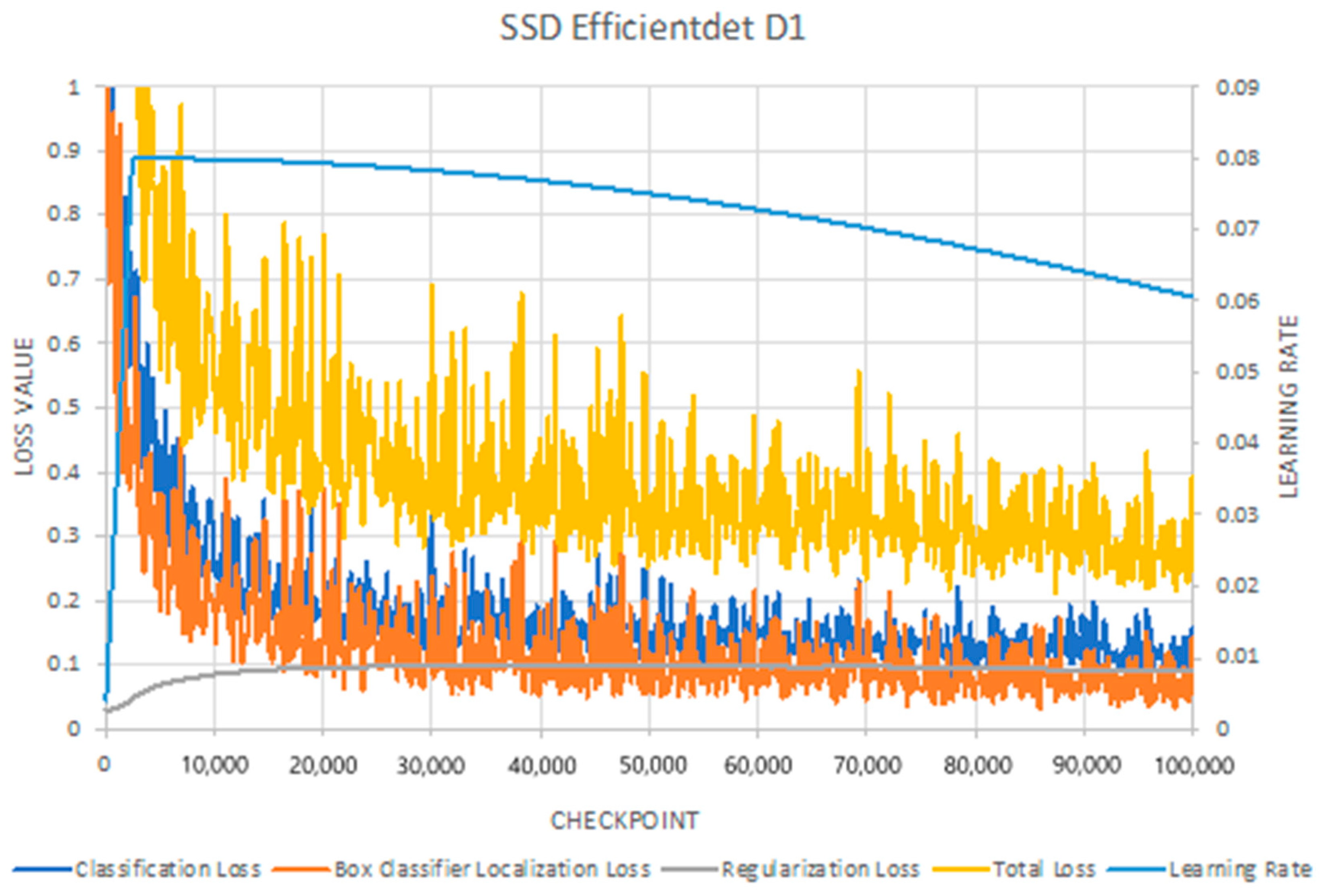
• Classification Loss: measures the difference between predicted class probabilities and the actual class labels and quantifies how well the predictions match the true class labels.
• Localization Loss: measures the discrepancy between the predicted bounding box coordinates and the ground truth bounding box coordinates.
• Regularization Loss: This term is added to the total loss function to prevent overfitting by penalising large weights or complex models and imposes constraints on model parameters to encourage the model to generalise unseen data better.
• Total Loss: represents the overall error, which typically combines various individual loss terms, such as classification, localisation, and regularisation loss, into a single scalar value.

Furthermore, as part of model evaluation, the selected framework provides various evaluation protocols as part of its Object Detection API. These protocols, including COCO Detection Metrics, PASCAL VOC 2010 detection metrics, and Open Images V2 Detection Metrics, provide detailed insights into a model’s performance in object detection tasks. Metrics such as Precision (mAP), Recall, and Average Precision (AP) are crucial in assessing the ability to localise and classify objects accurately across different datasets.

• The COCO detection metrics include:
  • Detection Boxes—Precision (mAP). It measures the average precision of object detection across multiple object categories. It evaluates how accurately the model localises and classifies objects within detected bounding boxes.
  • Detection Boxes—Recall. It evaluates the model’s ability to detect all relevant objects within an image. It measures the proportion of true positive detections out of all actual positive instances in the dataset.
  • Losses (classification, localisation, regularisation and total).
• The PASCAL VOC 2010 detection metrics include:
  • Performance per class—Average Precision (AP) is calculated individually for each object class present in the dataset. It provides insights into the model’s performance in detecting and classifying objects of specific categories.
  • Precision (mAP)—Mean Average Precision (mAP) evaluates the overall precision of object detection across all object classes. It computes the average AP scores for each class, providing a comprehensive measure of the model’s detection accuracy.
• Open Images V2 Detection
  • This metric includes the same metrics (AP and mAP) as the PASCAL VOC 2010 metric. However, the primary distinction lies in the criteria used to classify detected boxes as TP, FP or ignored.

2.2.3. Model Testing

Evaluating the performance of a model involves predicting new datasets and using specific metrics focusing on various behaviours. This section presents the methods used for evaluation tailored explicitly for multi-class classification scenarios [26], which differ from binary classification approaches.

• Confusion Matrix
  The Confusion Matrix displays predicted versus expected information, revealing where and how the model becomes confused. This analysis focuses solely on the multiclass classification scenario (

  Table 5. Multi-class confusion matrix ¹.

  Predicted	Expected
  	A	B	C	D	E	Not Detected
  A	AA	BA	CA	DA	EA	!A
  B	AB	BB	CB	DB	EB	!B
  C	AC	BC	CC	DC	EC	!C
  D	AD	BD	CD	DD	ED	!D
  E	AE	BE	CE	DE	EE	!E

  ¹ The ! symbol in the “Not Detected” column represents the Boolean NOT operator.

  ). Before delving into further details, the following terms need to be defined:
  • True Positive (TP) refers to instances where the model correctly detects the target object and the predicted class matches the ground truth class e.g., in the A class, TP_A = AA;
  • False Positives (FPs) refer to instances where the model correctly detects the target object; however, misclassification occurs e.g., in the A class, FP_A = BA + CA + DA + EA;
  • False Negative (FN) refers to instances where the model fails to detect the target object (red) or is incorrectly classified e.g., in the A class, FN_A = !A + AB + AC + AD + AE;
  • True Negative (TN) in multiclass classification is a complex case, and it is computed by summing all instances where the model correctly predicts classes other than the true positive class e.g., in the A class, TN_A = BB + CB + DB + EB + BC + CC + DC + EC + BD + CD + DD + ED + BE + CE + DE + EE.

The confusion matrix should be transformed into a one-versus-all matrix for each class, also known as a binary-class confusion matrix (

Table 6. Binary-class confusion matrix.

Predicted	Expected
	Positive	Negative
Positive	TP	FP
Negative	FN	TN

). This matrix is utilised to compute class-wise metrics such as precision, recall, and accuracy.

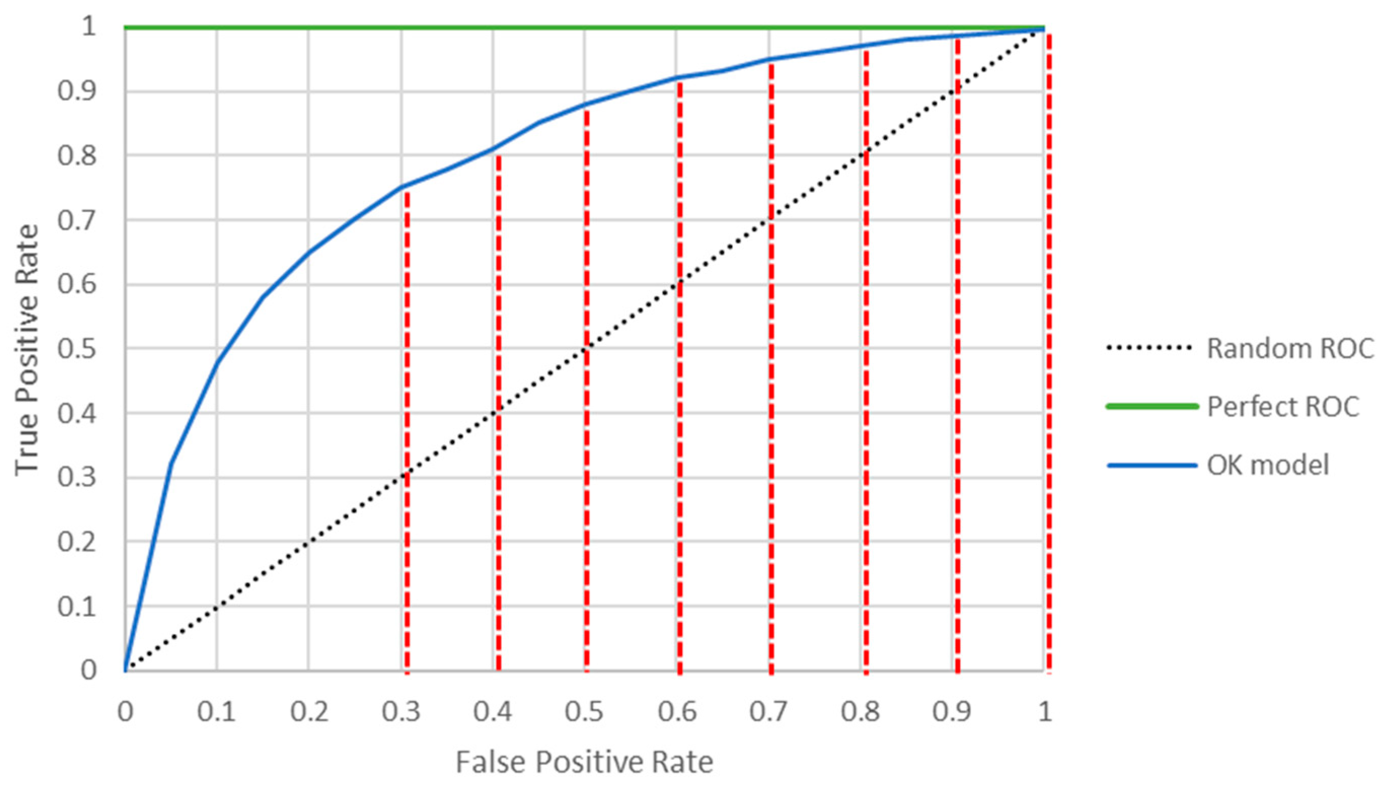
• Receiver Operating Characteristics (ROC) Curve and Area Under the Curve (AUC)

The performance of a model can be evaluated using the ROC curve. This graphical representation plots the true positive rate (TPR), also known as Recall or Sensitivity, on the y-axis and the false positive rate (FPR) on the x-axis at different Intersections over Union (IoU) thresholds. These rates are calculated based on the Equations (1) and (2). The ROC curve is a valuable tool in assessing the trade-off between TPR and FPR and is commonly used to evaluate classification models’ performance.

$$TPR={\displaystyle \frac{TP}{TP+FN}}$$

(1)

$$FPR={\displaystyle \frac{FP}{FP+TN}}$$

(2)

The ROC graph, as depicted in Figure 3, serves as a standard tool for assessing the performance of the models. In every ROC graph, the reference point is the random diagonal ROC line, representing a model that predicts classes with equal probability. Anything below this line signifies inefficiency in classification. In an ideal scenario where the model makes all predictions correctly, the ROC curve resembles the one depicted in green. In this case, the FPR consistently remains at 0, while the TPR remains at 1.0. However, the ROC curve typically falls between these two extreme cases, as represented by the blue curve. The AUC of the ROC curve is a single value used to evaluate the model’s performance. It quantifies the model’s ability to distinguish between classes across all possible thresholds.

• Intersection over Union

The Intersection over Union (IoU) is a fundamental evaluation metric in object detection tasks. It quantifies the accuracy of an object detection model by comparing the coordinates of both the ground-truth bounding box and the predicted bounding box (Figure 4). The IoU algorithm computes the ratio of the intersection area between these two bounding boxes to the area of their union. This resulting value measures how well the predicted bounding box aligns with the ground truth. IoU is commonly used as a threshold in determining whether a detected object is considered a true positive or a false positive, thus playing a crucial role in assessing the performance of object detection models.

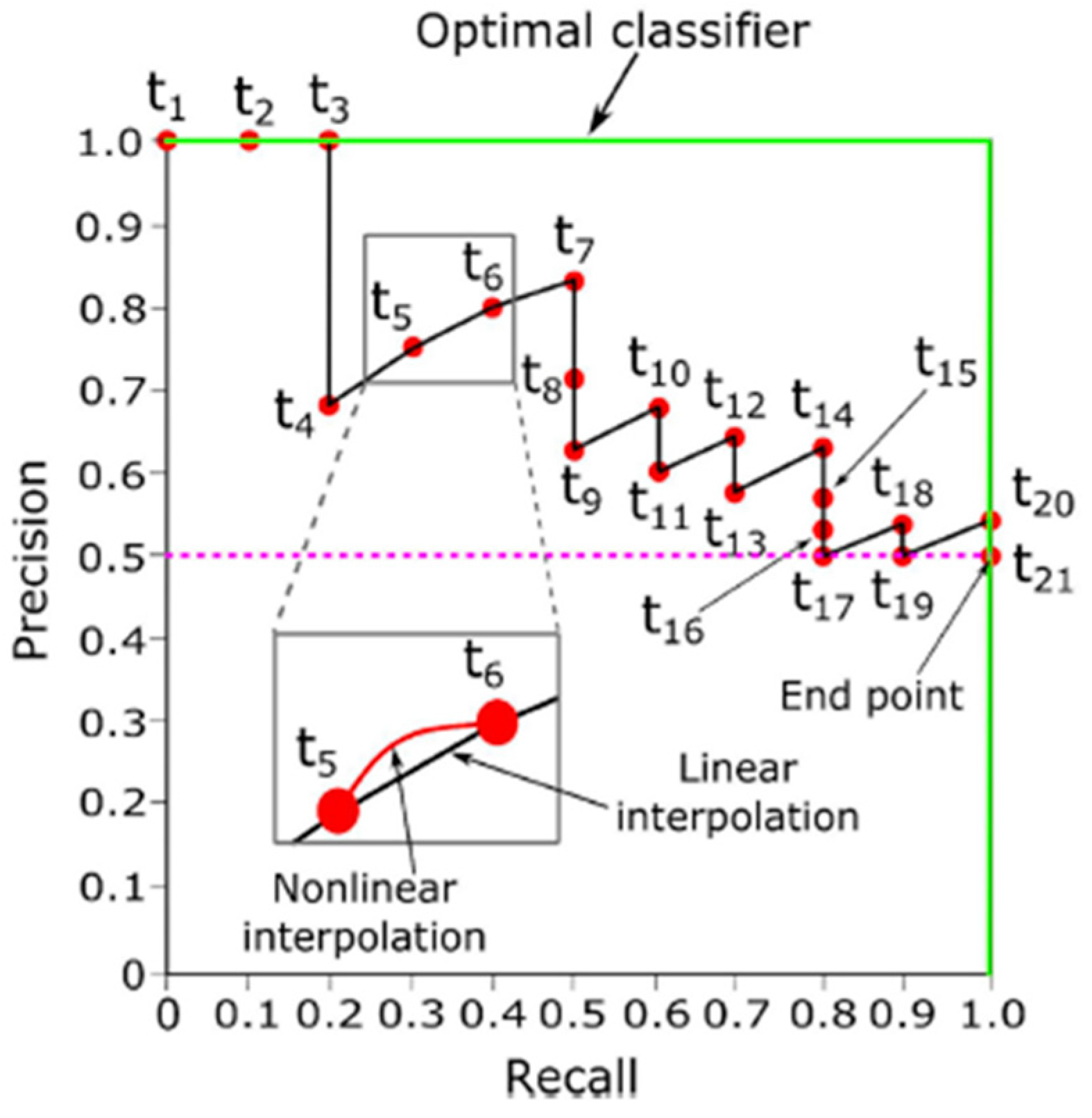
• Precision–Recall (PR)

The PR metric is another critical tool for evaluating model performance, particularly in scenarios characterised by class imbalance. Precision is a measure of result relevancy, thereby emphasising the accuracy of the model’s predictions. In contrast, recall measures the ability of the model to capture all relevant instances, reflecting the completeness of the retrieval process. Together, precision and recall offer valuable insights into the effectiveness of predictive models. These metrics are calculated based on the Equations (3) and (4):

$$P={\displaystyle \frac{TP}{TP+FP}}$$

(3)

$$R={\displaystyle \frac{TP}{TP+FN}}$$

(4)

The PR curve aligns with the rationale of the ROC Curve. However, recall is plotted on the x-axis in the PR curve, while precision is on the y-axis. Unlike the ROC curve, which accounts for TN values, the PR curve focuses solely on TP, FP, and FN values. This distinction renders the PR curve particularly valuable in scenarios with class imbalances, offering insights into precision–recall trade-offs across various IoU thresholds. Figure 5 shows an illustrative example of a PR curve. It often presents as a zigzag pattern and may intersect itself. The green line denotes ideal classification performance, achieving 100% precision and recall, while the purple line represents the baseline. Any points below the baseline signify inefficiency in classification.

• F1 score

The F1 score combines precision and recall into a single value, providing a balanced measure of a model’s performance. It is calculated based on Equation (5) as the harmonic mean of precision and recall. The F1 score ranges from 0 to 1, with higher values indicating better model performance. It is particularly useful in scenarios where precision and recall are essential and must be balanced.

$$F1={\displaystyle \frac{2TP}{2TP+FP+FN}}$$

(5)

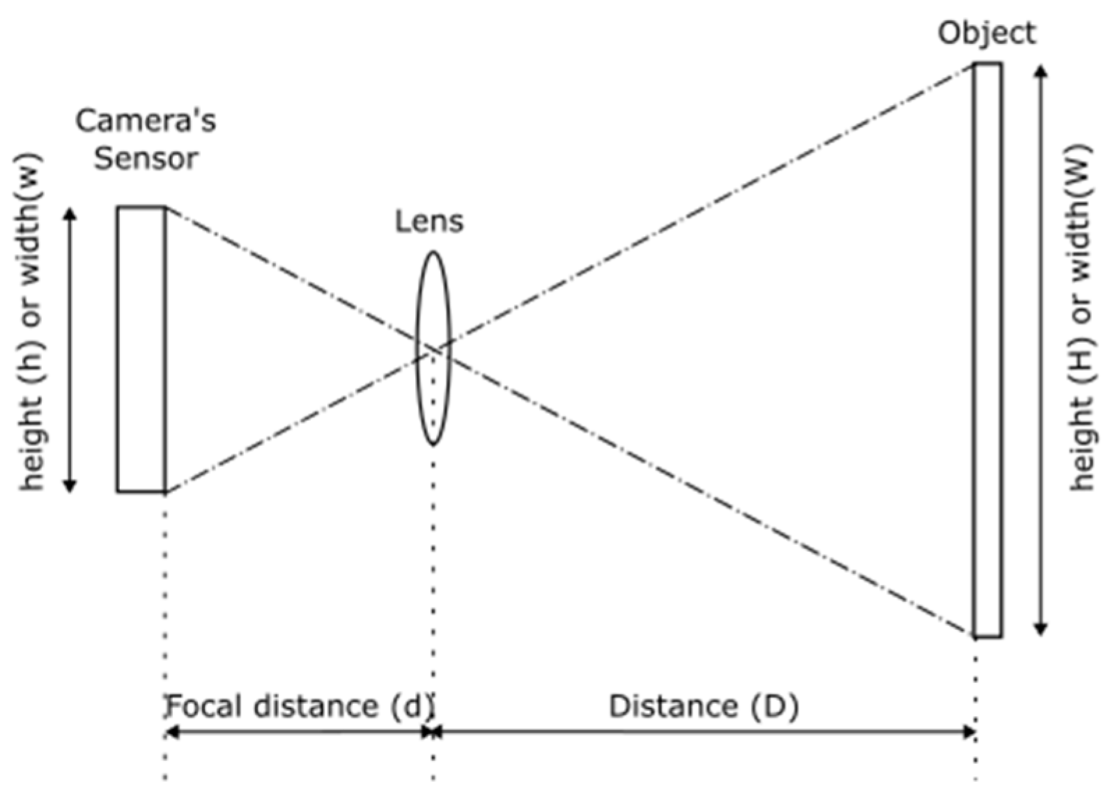
2.3. Defect Size Estimation

The scope of the proposed solution was to provide a more helpful tool to the maintenance personnel. In this context, a method was developed to estimate the size of the identified defects. The final goal is not only to calculate the size of the defect but also to monitor the degradation to see if it is something that dynamically evolves over time. The size estimation of the defect should be regarded as an indicative number as the procedure of measuring an artefact like a dent is a pedantic methodology that follows specific rules, and only trained maintenance engineers have the skills to accomplish that. However, the quantitative approach has its value since it can add to the data available for the maintenance personnel to assess the severity of the situation and its progression.

The developed approach takes into account specific considerations that need to be met in order to estimate the size of the defect. The still photos must be assumed to have been taken by a known camera and a drone equipped with a Light Detection and Ranging device (LIDAR). Regarding the first requirement, it is straightforward to believe that the camera characteristics are known, such as the height and width of the sensor and the focal length. The second requirement is the trickiest point since the distance definition cannot be defined accurately. In the working scenario, the assumption is that the distance between the drone and the aircraft’s surface is known but not between the drone and the specific artefact. However, it is still a good approximation since the flight path is a predefined perimetric trajectory that ensures that the drone always faces the surface perpendicularly and not at arbitrary angles. The industrial inspection drones employed for these tasks are equipped with 3D lidars that report back the distances as point clouds. The distance in the front direction that coincides with the visual camera is known and can be recorded as metadata of the still photo. Overall, it is apparent that the primary source of uncertainty is the distance estimation that affects the defect’s size calculation.

In the suggested approach, the workflow generates a bounding box after the defect detection, which becomes the region of interest. With the specific image section and the camera parameters (focal length, distance from camera, sensor height and width), the image is further processed to detect and analyse any defects present. The method first converts the image to grayscale and applies Gaussian blurring to smooth out noise. It then uses Canny edge detection to identify the edges in the image section, followed by dilation and erosion operations to clean up the edges.

The method finds all the contours in the processed image section and iterates through them. The contours detected within the input image section are indicative of potential defects. The dominant one is the defect candidate, which has an oval-like shape that is the most likely for the dents. For each contour with a sufficiently large area (greater than 10 pixels), the sizing method is used to measure the dimensions of the detected defect. It first orders the points of the contour to ensure they are in the correct order (top-left, top-right, bottom-right, bottom-left). It then calculates the midpoints between these points and uses the Euclidean distance between them to determine the width and height of the defect.

In calculating, the actual physical dimensions of the defect, the method uses the provided camera parameters (focal length, distance from camera, sensor height and width) along with the image dimensions to convert the pixel-based measurements to real-world units (millimetres). The calculation is straightforward using similar triangles as depicted in Figure 6, simplified for one dimension (vertical height). Equation (6) illustrates the calculation for the width.

$${defect}_w={\displaystyle \frac{D·dA·senso{r}_w}{f·imag{e}_w}}={\displaystyle \frac{D·dA}{EFL}}$$

(6)

In Equation (6), the defect width (defect_w) is given by the division of the product of the distance from the camera (D), the Euclidean distance between the midpoints for the width of the defect contour (dA), and the sensor’s width (sensor_w) divided by the product of the focal length (f) and the image’s width in pixels (image_w). By analysing this equation further, the Effective Focal Length (EFL) concept was identified. In computer vision, the EFL is crucial for understanding how a camera maps 3D scenes to 2D images. To map pixels to real-world distances, the relationship (Equation (7)) between the image size in pixels and the sensor’s physical size is crucial to allow us to relate pixel distances to real-world distances.

$$EFL={\displaystyle \frac{f·{image}_w}{{sensor}_w}}$$

(7)

The distance from the object is estimated using feedback from the lidar. The height of the sensor is determined by the contour pixels distance, and the focal length is reported in the metadata. Finally, the image displays the calculated dimensions using OpenCV’s text rendering capabilities. Overall, this approach provides a promising tool for analysing and measuring defects in images, leveraging computer vision techniques and camera parameters to provide representative size estimations.

3. Discussion

3.1. Defect Detection Results

This section analyses the model development procedure, providing insights into their performance and associated results. As previously outlined, the annotated dataset underwent testing against 11 pre-trained TensorFlow object detection models. Following an initial assessment, only the top five best-performing models were selected for further analysis. This chapter is structured into three sections: training, validation, and testing results. In the training and validation analysis, the focus is on the best-performing model. The same methodology was followed for the remaining four models but is not presented because of space considerations.

3.1.1. Training Analysis

The critical training metrics for evaluating the training process include classification, localisation, regularisation, total loss, as well as learning rate. Throughout the training process, the main goal was to maintain a balance between overfitting and underfitting. Monitoring the losses during training is essential to ensure they follow a descending trend, indicating that the model continues learning. If the training metrics stabilise or show an ascending trend, it indicates overfitting, and the training process should be stopped. Fluctuations are normal, signifying the model’s ongoing learning efforts, especially when a descending trend is observed.

Figure 7 illustrates the training performance of the SSD Efficientdet D1 model. The left Y-axis represents the loss metrics, while the right Y-axis denotes the learning rate. The X-axis spans from 0 to 100,000 steps, covering the training duration. Initially, the learning rate was set at a conservative value of 0.001 and gradually increased (warm-up phase) to the target value of 0.08. This technique of gradual adjustment aids in smoother optimisation, which is advantageous for complex datasets. As the training proceeds, the learning rate stabilises briefly before entering the descending phase, a common strategy to fine-tune model parameters and enhance convergence. At the same time, it can be noticed that the classification loss, localisation loss, and total loss exhibit a descending trend with fluctuations of up to 50,000 steps, indicative of the model’s learning process. The stabilisation, after that, signifies the optimisation and attainment of its potential capabilities. Regularization Loss, which is crucial for understanding generalisation, initially increased as the model learns from data, promoting better generalisation and mitigating overfitting. Following the same logic, it was stabilised as the model optimised its parameters and gradually decreased towards the training’s conclusion, reflecting convergence. Figure 7 shows that the SSD Efficientdet D1 model demonstrates a solid generalisation ability.

3.1.2. Validation Results

The models were trained using batches of images. The step, or iteration, refers to one update of the model’s parameters based on a batch of data. To fine-tune the training, 100 checkpoints were created for every 1000 steps. A validation check was performed at each checkpoint, leading us to create the comprehensive Figure 8. This graph showcases various metrics such as precision, recall, and losses, providing a clear picture of the trained model’s performance at each checkpoint. The left Y-axis represents precision and recall values, while the right Y-axis highlights the loss values. The X-axis, spanning from 0 to 100,000 steps, covers the entire training process.

Among the 100 checkpoints, fourteen specific sample points were selected and exported for further analysis to evaluate the model’s performance. The selection of these sample points was not random but based on the validation metrics mentioned earlier. In general, the criterion for selection involved identifying sample points with the lowest loss values and the highest precision and recall values, as this combination represents the ideal sample point.

In order to facilitate the checkpoint selection, the Precision/Recall Curve and ROC Curve were generated (Figure 9) to compare the model’s performance at each sample point. Analysis of the Precision/Recall curve reveals that step 47,000 exhibits the best performance, with an Average Precision of 0.28. Similarly, the ROC curve validates these findings, with an AUC of 0.66, indicating that step 47,000 achieves the best performance.

3.1.3. Testing Results

During the testing phase, the performance of each model was assessed using metrics such as the confusion matrix, precision, recall, F1 score, and AUC score. The top five models competed against each other to identify the best-performing model. A ROC curve and a Precision–Recall curve were computed for this process. After identifying the best-performing model, a detailed analysis was followed. It is worth mentioning that the same approach was applied across all five models, but it will not be presented to avoid redundancy.

A total of 150 images were allocated for the testing phase assessing the performance in new unseen images and understanding each model’s strengths and weaknesses was straightforward. Compiling the testing metrics into a single table allowed for a clear comparison of the performance, ensuring fairness in assessing them based on the specific conditions outlined in the methodology section.

Table 7. The metrics related to dent class detection for the fivetop-performing models.

Model	Dent Precision	Dent Recall	Dent F1	Average AUC	Average Precision	Average F1
EfficientDet D1	0.712	0.439	0.543	0.657	0.279	0.526
EfficientDet D0	0.652	0.450	0.533	0.641	0.261	0.473
Faster R-CNN ResNet50 V1	0.565	0.357	0.438	0.608	0.229	0.444
SSD ResNet50 V1 FPN	0.710	0.407	0.518	0.590	0.214	0.411
Faster R-CNN ResNet50 V1	0.500	0.290	0.367	0.607	0.228	0.407

presents the dent’s precision, recall, and F1 score alongside the average AUC score, precision score, and F1 score. Apart from the dent-recall metric, ssd_efficientdet_d1 consistently outperformed the other models across all test metrics. The ssd_efficientdet_d0 model closely follows, demonstrating significant performance over the remaining three models. This finding suggests that the ssd_efficientdet dataset was better suited to the dataset, and the optimisation of model training contributed to its superior performance compared to the other models. Additionally, the ssd_efficientdet architecture, combining SSD with an EfficientNet-b1 backbone and BiFPN feature extractor, proved highly adaptable to the dataset.

A better visualisation to compare the performance of all models is the utilisation of the ROC and PR curves (Figure 10). These graphs further support the conclusions drawn from the comparison table, highlighting the superior performance of ssd_efficientdet d1 and d0 over the other three models. Unlike the tabulated results, which were derived using mathematical formulas, these curves offer a graphical representation of model performance. Additionally, the consistency between manually calculated AUC scores and AP scores and those generated computationally confirms the accuracy of the findings.

The previous section’s comparison analysis shows that the best-performing model is the Efficientdet d1. For this model, the resolution of the presented analysis will be increased, going deeper and understanding the behaviour of the model for the different types of artefacts. A precision–recall curve was generated using a stringent IOU threshold set at 0.9 to achieve this. As depicted in Figure 11, both the precision and recall axes range from 0 to 1. Notably, the class exhibiting the best performance is missing paint and repair, with an average precision (AP) of 0.49, while dent ranks fourth, boasting an AP of 0.44. This performance discrepancy can be attributed to missing paint and screws, which are classes with a higher number of annotations compared to dents, repairs, and scratches. To enhance precision and recall scores, augmenting the sample size for the underrepresented classes is imperative. An additional reason that justifies this behaviour is that repairs and screws carry significantly more visual information compared to a dent (e.g., a screw has the characteristic shape of a circle with a cross in the centre).

The ROC curve and its associated AUC score offer an alternative method to assess the performance of the model for each class. Similar to the precision–recall curve, the IOU threshold remained fixed at 0.9, indicating a strict requirement for proximity between the ground-truth bounding box and the predicted bounding box to validate a prediction. In contrast to the PR curve, the ROC curve displays slight variations in the performance of each class. This discrepancy arises from consideration of both negative and positive instances, unlike the PR curve, which solely focuses on positive instances. Consequently, the PR curve proves more suitable for evaluating an imbalanced dataset, such as the one utilised in our experiment.

When analysing Figure 12, it is evident that the class for the repairs attains the highest AUC score of 0.78, followed by the dent class with an AUC score of 0.69, and the screw class ranks third with a score of 0.68. Comparing the ROC curves of all five classes with the baseline, it becomes apparent that the model’s performance is notably robust, showcasing high TPRs coupled with low FPRs.

The Confusion Matrix is an essential quantitative method for analysing the performance of the model. The analysis focuses on dent detection; consequently, the description presented below is specific to dents, accompanied by some average metrics (

Table 8. Multiclass confusion matrix.

Predicted	Expected
	Dent	Missing Paint	Screw	Repair	Scratch	Not Detected
Dent	47	5	3	8	3	50
Missing paint	4	81	11	3	13	93
Screw	1	10	79	10	4	86
Repair	5	4	8	62	0	25
Scratch	0	6	4	3	17	23

,

Table 9. The binary confusion matrix focused on the dents.

Predicted Dent	Expected Dent
	Positive	Negative
Positive	47	19
Negative	60	542

and

Table 10. The performance metrics focused on the dents.

Class Name	TRP	FPR	Precision	Recall	AP	F1	AUC	CL-Min	CL-Avg	CL-Max
Dent	0.44	0.03	0.71	0.44	0.44	0.54	0.69	20	59	98
Average					0.28	0.53	0.66

). The model successfully identified 47 out of 116 dents, with 50 cases being missed and 19 instances of misclassification. Furthermore, the precision level stood at 0.71, while the recall was 0.44, indicating that nearly half of the cases were accurately detected and classified. Another significant metric is the confidence level (CL), averaging 59%, with a minimum of 20% and a maximum of 98%. On average, the model exhibited a precision of 0.28, an AUC level of 0.66, and an F1 score of 0.53. Considering the dataset’s complexity, the physical attributes of the dent class, and the environmental conditions during image capture, the model’s performance can be characterised as a high-precision model with moderate recall levels, capable of detecting various object sizes across diverse environmental conditions.

Another metric calculated for the best-performing model was the average precision–recall curve and the ROC curve (Figure 13). This is useful because it can be used to compare the performance of each model against one another using single scores like AP and AUC instead of per class. In this case, to compute the average in both instances, we utilised the macro method, where all the scores for each class were summed and then divided by the total number of classes. Regarding Average Precision (AP), the average score was 0.42, and the Area Under the Curve (AUC) score was 0.69.

Another observation is related to the shape of the two lines: the precision–recall curve forms almost a straight line, indicating a stable model that makes consistent predictions regardless of the chosen threshold. Additionally, a ROC curve, exhibiting an initial sharp increase followed by a relatively constant rise for the remaining thresholds, suggests a model with discriminatory solid power across a range of thresholds, making it effective at distinguishing between positive and negative instances.

3.1.4. Limitations and Possible Improvements in Defect Detection

The results achieved using the developed models are not indicative of the success rate of a potential product-grade solution. However, during the testing phase, the performance metrics achieved are promising, prompting consideration of necessary improvements to enhance the quality of the results. As previously mentioned, the focus of the tests was to identify dents, which are the most challenging yet one of the most wanted in the industry. In testing results, the performance was compared with the baseline. In this case, the baseline can be regarded as a human’s ability to identify dents. In [27], See suggested in their research that the error level in manual aircraft visual inspection is 32%. From discussions with TUI’s experienced technicians, this is a very challenging task carried out by certified personnel and often involves using torches or changing the angle of view to identify discontinuities in the reflections. In addition, the decision to move closer to real-world applications rather than taking focused pictures without background makes the operational scenario more challenging but equally more convincing for the credibility of the solution. The straightforward, immediate actions that can be implemented to improve the results are the following:

• Increase the number of annotations: This is important for creating a more robust and balanced dataset. Ensuring enough examples of each class helps prevent bias and improves the model’s generalisation ability.
• Consistent image capture: Using the same sensor and shooting conditions helps maintain consistency across the dataset. This reduces variability and ensures the model learns features relevant to the objects rather than environmental factors.
• Capture variations: Taking images of the same object from different angles and under different environmental conditions helps the model learn to recognise objects in various contexts, improving its robustness.
• Image processing: Adjusting exposure levels can help enhance features and remove unnecessary information, making detecting objects more accessible for the model. However, it is essential to ensure that these modifications do not distort the objects or introduce artefacts that could confuse the model.
• Oriented bounding boxes: Oriented bounding boxes can improve localisation accuracy, especially for objects with non-standard orientations. This helps the model better understand the spatial layout of objects in the image.

3.2. Defect Size Estimation Results

3.2.1. Lab Tests

Having theatrically formed a procedure that estimates the dimensions of an object, in this case, a defect, validation tests were performed in a lab environment. A standard DSLR camera and a compact optical distance measurement sensor (LIDAR-Lite) were used. In the lab, the experiment setup focused on validating the concept. In the lab, the experiment setup focused on validating the concept. A Python script was developed using the OpenCV library and a minimal graphical user interface to draw the bounding box instead of connecting an object detector. The tests reported encouraging results using different objects or drawings and taking photos in perpendicular positions (Figure 14).

The experiment flow was to select a camera, where characteristics such as the focal length and sensors’ dimensions were hard coded, upload the image, draw a bounding box with the mouse, and press the size estimation button. The achieved results showed a minor deviation from the expected ones (

Table 11. Sample width and height measurements for objects in the lab.

Object	Actual (mm)	Measured (mm)	Abs Difference (mm)
object 1 width	88.5	88.5	0.0
object 1 height	53.5	53.6	0.1
object 2 width	150.0	147.9	2.1
object 2 height	70.0	72.7	2.7
object 3 width	150.0	149.2	0.8
object 3 height	62.0	62.2	0.2
object 4 width	8.0	8.2	0.2
object 4 height	7.4	8.1	0.7
object 5 width	23.6	21.1	2.5
object 5 height	23.1	21.0	2.1
object 6 width	79.5	79.0	0.5
object 6 height	76.2	79.0	2.8

). The ground truth of the dimension was measured using a ruler, which is also an error-prone manual method. The results were encouraging, although the hangar test was expected to be much more challenging.

3.2.2. Hangar Tests

With the lab tests completed, the focus was moved to the hangar tests regarding the assessment of the size estimation procedure. It was impossible to carry out those tests using the COTS drone in TUI’s hangar because there was no suitable sensor to measure the distance from the aircraft. The experiments took place in the DARTeC smart hangar using our ground demonstrator Boeing 737-400. The replication of the size estimation of the defect was not straightforward. A tripod was used to mount the camera and a handheld laser sensor to imitate the concept of a lidar-equipped UAV. The laser sensor was the weakest link in the suggested work assumption since it was unreliable, introducing error-prone distance estimations.

Figure 15 illustrates a couple of application examples. In the first one, a potential point of failure was identified. As described in the methodology, the defect is approximated by fitting a contour, and then its width and height are estimated. In this case, the colour transition (spatial frequency) of the area of interest was low, and the algorithm mistakenly focused on a false artefact, conveying incorrect feedback. In the second example, that algorithm worked as expected. In all cases where the artefact was clearly visible, the contour approximation was correct. In terms of accuracy,

Table 12. Defect width and height measurements for dents in the hangar. ADDED.

Object	Actual (mm)	Measured (mm)	Abs Difference (mm)
defect 1 width	73	60.5	12.5
defect 1 height	94	74.1	19.9
defect 2 width	130	113.9	16.1
defect 2 height	90	74.7	15.3
defect 3 width	110	143.9	33.9
defect 3 height	75	95.9	20.9
defect 4 width	65	80.1	15.1
defect 4 height	75	106.7	31.7
defect 5 width	190	145.5	44.5
defect 5 height	65	94.3	29.3

illustrates a few examples of defect size estimations and the absolute difference compared to the estimated dimensions. It was noticed that even a slight movement of the measuring device changes the distance of the recorded error non-linearly. The same thing applies also by changing the angle at which the laser device is placed in reference to the defect. Additionally, it worked better when the image was focused perpendicularly to the defect resembling the lab tests. Unfortunately, estimating a solid and consistent error deviation of the procedure since the error fluctuated heavily and was affected by the error-prone distance estimation, the position of capture, and additional factors addressed in the discussion of limitations and possible improvements section.

In the hangar experiments, it was realised that the distance measurement was the primary source of instability. Therefore, it would be enlightening to perform some tests and identify the behaviour of the point laser device in a representative environment. The aim of the tests was to assess the accuracy of the device at different distances, angles, and materials (reflective and non-reflective). In the first experiment (Figure 16a), the device was tried in vertical mode, targeting non-reflective surfaces (

Table 13. Laser device pointing perpendicular to a non-reflective surface.

Distance (cm)	Distance Measured (cm)	Difference (cm)
30	34	4 (close to dead zone)
60	60	0
100	100	0
250	250	0
400	402	2
500	501	1

).

In the next experiment, the device was placed at different angles with reference to the surface where the target exists. The first choice was perpendicular to the surface (90 degrees), and the second was at a 45-degree angle (Figure 16b,c). The experiment was repeated twice for reflective and non-reflective surfaces (

Table 14. Laser device experiments pointing reflective and non-reflective surfaces, targeting the surface at 45 and 90 degrees.

Distance (cm)	Angle (Degrees)	Material	Distance Measured (cm)	Difference (cm)
100	90	non-reflective	100	0
100	45	non-reflective	101	1
100	90	reflective	101	1
100	45	reflective	135	35

).

The results illustrated that the reported value was volatile when used on reflective surfaces like the aircraft’s skin and when the device and the artefact were not in a perpendicular direction. This behaviour justifies the erratic estimations recorded during the hangar experiments targeting a reflective surface at various angles.

3.2.3. Limitations and Possible Improvements in Size Estimation

The size estimation procedure proved effective in the lab experiments but exhibited instability in the hangar. The following list sheds light on the factors affecting the proposed approach, and by addressing them, the reliability of the solution will be enhanced.

• In some cases, the contour approximation used in the sizing estimation fails to identify dents that are not clearly visible in the photo. If there is a visible colour change that creates an edge, it gives promising results.
• The suggested area of interest (bounding box), which comes from the defect detector, sometimes crops out part of the dent, directly affecting the size estimation. The defect detector works in a stringent IOU (0.9), which is advantageous for the sizing algorithm. The introduction of oriented rounded boxes could further improve the situation.
• There is no solid reference to compare. Trained maintenance engineers perform dent sizing, but the research team lacks this expertise. The manual measurement was not industry-accepted at this stage and introduced uncertainty as it cannot be considered a solid ground truth.
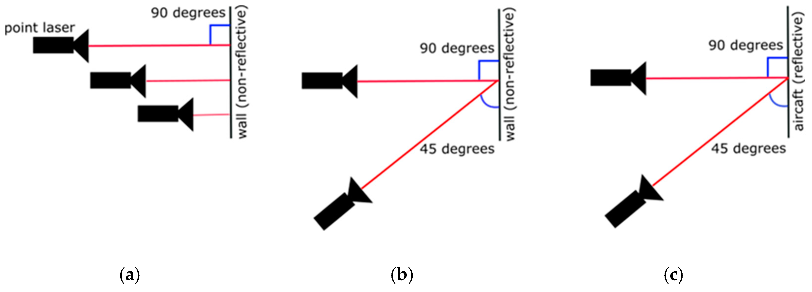
• The distance in the experiments was measured by a laser distance measurer, which, most of the time, did not work because of the reflection on the aircraft’s skin, so instead, a tape measure was used. This procedure is far from perfect. However, in the actual scenario, the UAV has a lidar and flies in a predefined path, maintaining a fixed distance from the aircraft. In addition, since the lidar emits beams on the surface (32 to 128, depending on the model). In this case, an area average can be used, rather than only one measurement utilised in the current experiment.
• If the photo capture is not perpendicular to the defect, perspective distortion may affect the size estimation.
• Lens distortion or image sensor characteristics introduce errors that need to be validated in the representative environment with the camera onboard the UAV.

4. Conclusions

The aviation industry is highly regulated, focusing on ensuring aircraft airworthiness and minimising the possibility of undetected defects. The first line of defence in maintenance is detailed inspection, with visual inspection accounting for nearly 80% of all inspections. The industry progresses towards MRO 4.0, which adopts machine learning, IoT sensors, and data analytics technologies, showing an increasing interest in using robotics and AI-based methods for defect detection. The research focused on detecting the location of defects on aircraft skin and estimating their size. The performance of various pre-trained CNN-based models was evaluated, focusing on the most challenging type of defect, dents. The best-performing model achieved 71% precision, with an area under the ROC curve of 0.69. In addition, the suggested size estimation approach was tested in the lab to prove the feasibility of the concept and then in the hangar. In the real-world environment, many factors were identified that influenced the estimation and made the estimation unreliable. Addressing these limitations following the suggested improvements will improve the overall estimation reliability.

References

1. IBISWorld. Global Airline Industry Market Size from 2018 to 2023 (in Billions of U.S. Dollars). 2023. Available online: https://www.statista.com/statistics/1110342/market-size-airline-industry-worldwide/ (accessed on 8 February 2024).
2. Federal Aviation Administration. Visual Inspection for Aircraft. In Advisory Circular ACNO; 1997; pp. 43–204. Available online: https://www.faa.gov/documentLibrary/media/Advisory_Circular/43-204.pdf (accessed on 9 September 2024).
3. Drury, C.G.; Watson, J. Good practices in visual inspection. In Human Factors in Aviation Maintenance-Phase Nine, Progress Report, FAA/Human Factors in Aviation Maintenance; Federal Aviation Administration (FAA): New York, NY, USA, 2002; Available online: https://dviaviation.com/files/45146949.pdf (accessed on 9 September 2024).
4. Civil Aviation Authority. CAP 562: Civil Aircraft Airworthiness Information and Procedures. 2020. Available online: http://publicapps.caa.co.uk/modalapplication.aspx?appid=11&mode=detail&id=92 (accessed on 8 February 2024).
5. Hrymak, V.; Codd, P. Improving Visual Inspection Reliability in Aircraft Maintenance. Conference Papers. 2021. Available online: https://arrow.tudublin.ie/beschreccon/153 (accessed on 8 February 2024).
6. Spencer, F. Visual Inspection Research Project Report on Benchmark Inspections. 1996. Available online: https://rosap.ntl.bts.gov/view/dot/12923 (accessed on 9 September 2024).
7. Donecle-Automating your Aircraft Inspections. Available online: https://www.donecle.com/ (accessed on 8 February 2024).
8. Mainblades-Drone Aircraft Inspections. Available online: https://mainblades.com/ (accessed on 8 February 2024).
9. Holl, J. Hangar of the future. Airbus. Available online: https://www.airbus.com/en/newsroom/news/2016-12-hangar-of-the-future (accessed on 19 June 2024).
10. Woodrow, B. EasyJet, Partners Developing UAS Aircraft Inspection Technology-Avionics International0. Avionics International. Available online: https://www.aviationtoday.com/2015/01/20/easyjet-partners-developing-uas-aircraft-inspection-technology/ (accessed on 10 May 2024).
11. Krizhevsky, A.; Sutskever, I.; Hinton, G.E. ImageNet Classification with Deep Convolutional Neural Networks. Adv. Neural Inf. Process Syst. 2012, 25. Available online: http://code.google.com/p/cuda-convnet/ (accessed on 10 May 2024). [CrossRef]
12. Malekzadeh, T.; Abdollahzadeh, M.; Nejati, H.; Cheung, N.-M. Aircraft Fuselage Defect Detection using Deep Neural Networks. 2017. Available online: https://arxiv.org/abs/1712.09213v2 (accessed on 13 February 2024).
13. Doğru, A.; Bouarfa, S.; Arizar, R.; Aydoğan, R. Using Convolutional Neural Networks to Automate Aircraft Maintenance Visual Inspection. Aerospace 2020, 7, 171. [Google Scholar] [CrossRef]
14. Bouarfa, S.; Doğru, A.; Arizar, R.; Aydoğan, R.; Serafico, J. Towards automated aircraft maintenance inspection. A use case of detecting aircraft dents using mask r-cnn. AIAA Scitech 2020 Forum 2020, 1. [Google Scholar] [CrossRef]
15. Yasuda, Y.D.V.; Cappabianco, F.A.M.; Martins, L.E.G.; Gripp, J.A.B. Automated Visual Inspection of Aircraft Exterior Using Deep Learning. In Proceedings of the Anais Estendidos da Conference on Graphics, Patterns and Images (SIBGRAPI), Gramado, Rio Grande do Sul, Brazil, 18 October 2021; pp. 173–176. [Google Scholar] [CrossRef]
16. Avdelidis, N.P.; Tsourdos, A.; Lafiosca, P.; Plaster, R.; Plaster, A.; Droznika, M. Defects Recognition Algorithm Development from Visual UAV Inspections. Sensors 2022, 22, 4682. [Google Scholar] [CrossRef] [PubMed]
17. Ren, I.; Zahiri, F.; Sutton, G.; Kurfess, T.; Saldana, C. A Deep Ensemble Classifier for Surface Defect Detection in Aircraft Visual Inspection. Smart Sustain. Manuf. Syst. 2020, 4, 81–94. [Google Scholar] [CrossRef]
18. Miranda, J.; Larnier, S.; Herbulot, A.; Devy, M. Uav-based inspection of airplane exterior screws with computer vision. In Proceedings of the VISIGRAPP 2019-Proceedings of the 14th International Joint Conference on Computer Vision, Imaging and Computer Graphics Theory and Applications, Prague, Czech Republic, 25–27 February 2019; Volume 4, pp. 421–427. [Google Scholar] [CrossRef]
19. Ding, M.; Wu, B.; Xu, J.; Kasule, A.N.; Zuo, H. Visual inspection of aircraft skin: Automated pixel-level defect detection by instance segmentation. Chin. J. Aeronaut. 2022, 35, 254–264. [Google Scholar] [CrossRef]
20. Redmon, J.; Divvala, S.; Girshick, R.; Farhadi, A. You Only Look Once: Unified, Real-Time Object Detection. In Proceedings of the IEEE Computer Society Conference on Computer Vision and Pattern Recognition, Las Vegas, NV, USA, 27–30 June 2016; pp. 779–788. [Google Scholar] [CrossRef]
21. He, K.; Gkioxari, G.; Dollár, P.; Girshick, R. Mask R-CNN. IEEE Trans. Pattern. Anal. Mach. Intell. 2017, 42, 386–397. [Google Scholar] [CrossRef] [PubMed]
22. Qu, Y.; Wang, C.; Xiao, Y.; Yu, J.; Chen, X.; Kong, Y. Optimization Algorithm for Surface Defect Detection of Aircraft Engine Components Based on YOLOv5. Appl. Sci. 2023, 13, 11344. [Google Scholar] [CrossRef]
23. Rice, M.; Li, L.; Ying, G.; Wan, M.; Lim, E.T.; Feng, G.; Ng, J.; Jin-Li, M.T.; Babu, V.S. Automating the Visual Inspection of Aircraft. In Proceedings of the Singapore Aerospace Technology and Engineering Conference (SATEC), Suntec Singapore Convention and Exhibition Centre, Singapore; 2018. Available online: https://oar.a-star.edu.sg/communities-collections/articles/13872?collectionId=20 (accessed on 8 February 2024).
24. Aust, J.; Shankland, S.; Pons, D.; Mukundan, R.; Mitrovic, A. Automated Defect Detection and Decision-Support in Gas Turbine Blade Inspection. Aerospace 2021, 8, 30. [Google Scholar] [CrossRef]
25. Yasuda, Y.D.V.; Cappabianco, F.A.M.; Martins, L.E.G.; Gripp, J.A.B. Aircraft visual inspection: A systematic literature review. Comput. Ind. 2022, 141, 103695. [Google Scholar] [CrossRef]
26. Tharwat, A. Classification assessment methods. Appl. Comput. Inform. 2021, 17, 168–192. [Google Scholar] [CrossRef]
27. See, J.E. Visual Inspection: A Review of the Literature; Sandia National Laoratories: Albuquerque, NM, USA, 2012; p. 87185. [Google Scholar] [CrossRef]
Figure 1. Data collection: (a) the Parrot Anafi drone (yellow frame) is flying inside TUI’s Group Hangar at Luton airport; (b) Boeing 737-400 ground demonstrator in Cranfield’s University DARTeC Smart Hangar.
Technologies 12 00158 g001
Figure 2. These are the five different classes that are considered in the approach: (a) dent; (b) missing paint; (c) screw; (d) repair, and (e) scratch.
Technologies 12 00158 g002
Figure 3. ROC curve.
Technologies 12 00158 g003
Figure 4. Intersection over Union.
Technologies 12 00158 g004
Figure 5. PR curve (image taken from [26]).
Technologies 12 00158 g005
Figure 6. The calculation of the object’s height using similar triangles knowing the focal distance, the distance from the object and the sensor’s height.
Technologies 12 00158 g006
Figure 7. The graph illustrates the classification, localisation, regularisation, total losses, and learning rate during the training process for the best-performing model.
Technologies 12 00158 g007
Figure 8. The performance of the SSD EfficineDet D1 model during the training (14 checkpoints).
Technologies 12 00158 g008
Figure 9. The curves graphs in different checkpoints: (a) PR curve; (b) ROC curve.
Technologies 12 00158 g009
Figure 10. The graphs illustrate the performance differences in the top 5 models: (a) PR curve; (b) ROC curve.
Technologies 12 00158 g010
Figure 11. The precision–recall graph illustrates the model’s performance for the different types of artefacts.
Technologies 12 00158 g011
Figure 12. The ROC curve illustrates the model’s performance for the different types of artefacts.
Technologies 12 00158 g012
Figure 13. Average metric curves for the best performing model: (a) macro-average PR curve; (b) macro-average ROC and AUC at IOU threshold 0.9.
Technologies 12 00158 g013
Figure 14. Different scale examples from the lab measurement tests: (a) card case; (b) small-sized curve; (c) medium-sized curve; (d) large-sized curve.
Technologies 12 00158 g014
Figure 15. Examples of defect detection and size estimation: (a) the contours-based approximation algorithm failed to capture the dent; (b) the contours-based approximation algorithm correctly identified the dent.
Technologies 12 00158 g015
Figure 16. (a) Test the device at different distances from the wall; (b,c) test the device at 45 and 90-degree angles towards non-reflective and reflective surfaces.
Technologies 12 00158 g016